| Issue |
A&A
Volume 550, February 2013
|
|
|---|---|---|
| Article Number | A10 | |
| Number of page(s) | 12 | |
| Section | Interstellar and circumstellar matter | |
| DOI | https://doi.org/10.1051/0004-6361/201218962 | |
| Published online | 18 January 2013 | |
The distribution of warm gas in the G327.3–0.6 massive star-forming region
1
Max-Planck-Institut für Radioastronomie,
Auf dem Hügel 69,
53121
Bonn,
Germany
e-mail: sleurini@mpifr.de
2
Univ. de Bordeaux, LAB, UMR 5804, 33270
Floirac,
France
3
CNRS, LAB, UMR 5804, 33270
Floirac,
France
4
SRON Netherlands Institute for Space Research,
PO Box 800, 9700 AV
Groningen, The
Netherlands
5
Kapteyn Astronomical Institute, University of
Groningen, PO Box
800, 9700 AV
Groningen, The
Netherlands
6
Leiden Observatory, Leiden University,
PO Box 9513, 2300 RA
Leiden, The
Netherlands
7
Max Planck Institut für Extraterrestrische Physik,
Giessenbachstrasse 1,
85748
Garching,
Germany
Received: 4 February 2012
Accepted: 9 November 2012
Aims. Most studies of high-mass star formation focus on massive and/or luminous clumps, but the physical properties of their larger scale environment are poorly known. In this work, we aim at characterising the effects of clustered star formation and feedback of massive stars on the surrounding medium by studying the distribution of warm gas through mid-J12CO and 13CO observations.
Methods. We present APEX 12CO(6–5), (7–6), 13CO(6–5), (8–7) and HIFI 13CO(10–9) maps of the star forming region G327.36–0.6 with a linear size of ~3 pc × 4 pc. We infer the physical properties of the emitting gas on large scales through a local thermodynamic equilibrium analysis, while we apply a more sophisticated large velocity gradient approach on selected positions.
Results. Maps of all lines are dominated in intensity by the photon dominated region around the Hii region G327.3–0.5. Mid-J12CO emission is detected over the whole extent of the maps with excitation temperatures ranging from 20 K up to 80 K in the gas around the Hii region, and H2 column densities from few 1021 cm-2 in the inter-clump gas to 3 × 1022 cm-2 towards the hot core G327.3–0.6. The warm gas (traced by 12 and 13CO(6–5) emission) is only a small percentage (~10%) of the total gas in the infrared dark cloud, while it reaches values up to ~35% of the total gas in the ring surrounding the Hii region. The 12CO ladders are qualitatively compatible with photon dominated region models for high density gas, but the much weaker than predicted 13CO emission suggests that it comes from a large number of clumps along the line of sight. All lines are detected in the inter-clump gas when averaged over a large region with an equivalent radius of 50′′(~0.8 pc), implying that the mid-J12CO and 13CO inter-clump emission is due to high density components with low filling factor. Finally, the detection of the 13CO(10–9) line allows to disentangle the effects of gas temperature and gas density on the CO emission, which are degenerate in the APEX observations alone.
Key words: stars: formation / HII regions / ISM: individual objects: G327.3 / 0.6
© ESO, 2013
1. Introduction
The influence of high-mass stars on the interstellar medium is tremendous. During their process of formation, they are sources of powerful, bipolar outflows (e.g., Beuther et al. 2002), their strong ultraviolet and far-ultraviolet radiation fields give rise to bright Hii and photon dominated regions (PDRs) and during their whole lifetime powerful stellar winds interact with the surroundings. Finally, their short life ends in a violent supernova explosion, injecting heavy elements into the interstellar medium and possibly triggering further star formation with the accompanying shocks. These are also the type of regions that dominate far-infrared observations of starburst galaxies.
Most studies of massive star formation focus on emission peaks at infrared or submillimetre wavelengths, which correspond to peaks in the temperature and/or mass distribution. The aim of our work is to characterise the effects of clustered star formation and feedback of massive stars on the surrounding medium. We have made APEX maps of three cluster-forming regions (G327.3–0.6, NGC6334 and W51) in mid-J12CO ((6–5) and (7–6)) and 13CO transitions ((6–5) and (8–7)) in order to have a direct measure of the excitation of the warm extended inter-clump gas between dense cores in the cluster (see for example Blitz & Stark 1986; Stutzki & Güsten 1990). Our sample of sources was chosen among six nearby cluster-forming clouds mapped in water and in the 13CO(10–9) transition as part of the Water in Star-Forming Regions with Herschel (WISH; van Dishoeck et al. 2011) guaranteed time key program (GT-KP) for the Herschel Space Observatory (Pilbratt et al. 2010).
In this paper, we present the 12CO and 13CO maps of the star-forming region G327.3–0.6 at a distance of 3.3 kpc (Urquhart et al. 2011, based on H i absorption). G327.3–0.6 is well suited to study cluster-forming clouds because of its relatively close distance and because several sources in different evolutionary phases coexist in a small region, as found by Wyrowski et al. (2006). Our maps (with a linear extension of ~3 pc × 4 pc) cover the Hii region G327.3–0.5 (Goss & Shaver 1970) associated with a luminous PDR, and an infrared dark cloud (IRDC; Wyrowski et al. 2006) hosting the bright hot core G327.3–0.6 (Gibb et al. 2000) and the extended green object (EGO) candidate G327.30–0.58 (Cyganowski et al. 2008). Extended green objects are identified through their extended 4.5 μm emission in the Spitzer IRAC2 band, which is believed to trace outflows from massive young stellar objects (YSOs; Cyganowski et al. 2008).
This paper is organised as follows: in Sect. 2 we present the APEX and Herschel1 observations of G327.3–0.6, in Sect. 3 we discuss the morphology and kinematics of the 12CO and 13CO emission, in Sect. 4 we investigate the physical conditions of the emitting gas. Finally, in Sect. 5 we discuss our results and compare to similar observations performed towards low- and high-mass star forming regions. Our results are summarised in Sect. 6.
2. Observations
2.1. APEX telescope
The CHAMP+ (Kasemann et al. 2006; Güsten et al. 2008) dual colour heterodyne array receiver of 7 pixels per frequency channel on the APEX telescope2 was used in September 2008 to simultaneously map the star-forming region G327.3–0.6 in the 12CO (6–5) and (7–6) lines and, in a second coverage, the 13CO (6–5) and (8–7) transitions. The region from the hot core in G327.3–006 to the H ii region G327.3–0.5 (Fig. 1) was covered with on-the-fly maps of 200′′ × 240′′ spaced by 4′′ in declination and right ascension.
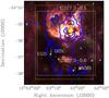 |
Fig. 1 Spitzer infrared colour image of the region G327.3–0.6 with red representing 8.0 μm, green 4.5 μm and blue 3.6 μm. The blue contours represent the integrated intensity of the 12CO(6–5) line (thin contours are 15%, 45% and 70% of the peak emission, thick contours 30%, 60% and 90% of the peak emission). The sources discussed in this paper (the IRDC, the EGO, the hot core G327.3–0.6, the SMM6 position and the Hii region G327.3–0.5) are also marked with crosses. The white and yellow boxes mark the regions mapped with APEX and Herschel, respectively. |
We used the fast Fourier transform spectrometer (FFTS, Klein et al. 2006) as backend with two units of fixed bandwidth of 1.5 GHz and 8192 channels per pixel. We used the two IF groups of the FFTS with an offset of ± 460 MHz between them. The original resolution of the dataset is 0.3 km s-1; the spectra were smoothed to 1 km s-1 for a better signal-to-noise ratio.
The observations were performed under good weather conditions with a precipitable water vapour level between 0.5 and 0.7 mm. Typical single side band system temperatures during the observations were around 1600 K and 5200 K, for the low and high frequency channel respectively. The conversion from antenna temperature units to brightness temperatures was done assuming a forward efficiency of 0.95 for all channels, and a main beam efficiency of 0.48 for the 12CO and 13CO (6–5) observations, 0.45 for the 12CO (7–6) data, and 0.44 for 13CO(8–7), as measured on Jupiter in September 20083. The pointing was checked on the continuum of the hot core G327.3–0.6 ( ). The maps were produced with the XY_MAP task of CLASS904, which convolves the data with a Gaussian of one third of the beam: the final angular resolution is 9
 4 for the low frequency data, 81 for the high frequency.
Observational parameters.
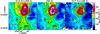 |
Fig. 2 Maps of the integrated intensity of the 12CO(3–2), (6–5) and (7–6) lines in the velocity range vLSR = [−54, −40] km s-1 (color scale). Solid contours are the integrated intensity of the 12CO(6–5) line from 20% of the peak emission in steps of 10%. In each panel, the positions analysed in Sect. 4.2 (the hot core, the IRDC position, and the centre of the Hii region) are marked with black triangles. The red star labels the position of the EGO. SMM6 (left panel) is one of the submillimetre sources detected by Minier et al. (2009). |
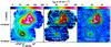 |
Fig. 3 Maps of the integrated intensity of the 13CO(6–5), (8–7) and (10–9) transitions in the velocity range vLSR = [−54, −40] km s-1 (colour scale). The solid contours in the left panel represent the LABOCA continuum emission at 870 μm from 5% of the peak emission in steps of 10% (Schuller et al. 2009). In the middle and right panels, the solid contours are the integrated intensity of the 13CO(6–5) from 20% of the peak emission in steps of 10%. In each panel, the positions analysed in Sect. 4.2 (the hot core, the IRDC position, and the centre of the Hii region) are marked with black triangles (except in the left panel, where the hot core is shown by a white triangle). The red star labels the position of the EGO. |
2.2. Herschel space observatory
The 13CO (10–9) line (see Table 1) was mapped (size = 210″ × 270″) with the HIFI instrument (de Graauw et al. 2010) towards G327.3-0.6 on February, 18th, 2011 (observing day – OD) 645, observing identification number (OBSID) 1342214421. The centre of the map is  . The observations are part of the WISH GT-KP (van Dishoeck et al. 2011). Data were taken simultaneously in H and V polarisations using both the acousto-optical Wide-Band Spectrometer (WBS) with 1.1 MHz resolution and the correlator-based high-resolution spectrometer (HRS) with 250 kHz nominal resolution. In this paper we present only the WBS data. We used the on-the-fly mapping mode with Nyquist sampling. HIFI receivers are double sideband with a sideband ratio close to unity. The double side band system temperatures and total integration times are respectively 384 K and 3482 s. The rms noise level at 1 km s-1 spectral resolution is ~0.1 K. Calibration of the raw data onto TA scale was performed by the in-orbit system (Roelfsema et al. 2012); conversion to Tmb was done with a beam efficiency of 0.74 and a forward efficiency of 0.96. The flux scale accuracy is estimated to be around 15% for band 3. Data calibration was performed in the Herschel Interactive Processing Environment (HIPE, Ott 2010) version 6.0. Further analysis was done within the CLASS90 package. After inspection, data from the two polarisations were averaged together.
The original angular resolution of the data is 190. The final maps were produced with the XY_MAP task of CLASS90 and have an angular resolution of 211.
3. Observational results
3.1. Morphology
Figure 1 shows the 12CO(6–5) integrated intensity map overlaid on the composite image of the IRAC Spitzer 3.6, 4.5 and 8.0 μm bands of the region. The 12CO emission traces the distribution of the 8.0 μm emission, but it is also associated with the infrared dark cloud found on the east of the hot core. The EGO candidate G327.30–0.58 identified by Cyganowski et al. (2008) and clearly visible in Fig. 1, is also detected in the 12CO data as secondary peak of emission (Fig. 2). The map of the integrated intensities of the 12CO(7–6) line is also presented in Fig. 2 together with the integrated intensity of the 12CO(3–2) line from Wyrowski et al. (2006). Figure 3 shows the distribution of the 13CO(6–5), (8–7) and (10–9) emissions. The accuracy of the relative pointings was checked on the hot core G327.3–0.6. For this purpose, we derived integrated intensity maps of lines detected only towards this position, which are close in frequency to the 12CO(6–5), 13CO(6–5) and 13CO(8–7) transitions, and therefore were observed simultaneously to the current dataset. From these data, we infer a position for the hot core in agreement with interferometric measurements at 3 mm (Wyrowski et al. 2008, and Table 2) within ~15.
All observed 12CO transitions trace the Hii region G327.3–0.5 as well as the infrared dark cloud which hosts the hot core G327.3–0.6. Moreover, the 12CO(6–5), (7–6) and 13CO(6–5) lines show extended emission along a ridge running approximately N-S that matches very well with the distribution of the CO(3–2) transition. The hourglass shape hole to the west of the Hii region G327.3–0.5 where the 12CO(3–2) emission is strongly reduced (see Wyrowski et al. 2006) is seen also in the 12CO(6–5) and (7–6) lines which, although much weaker than in the rest of the map, are still detected at this position.
All transitions peak towards the Hii region G327.3–0.5 where the main isotopologue lines have intensities up to 60–65 K. The integrated intensities of the CO isotopologues show a distribution along a ring-like structure around the peak of the cm continuum emission (Goss & Shaver 1970). The centre of the ring also coincides with the massive young stellar object number 87 identified in the near-infrared by Moisés et al. (2011). Since the ring is detected also in high-J transitions of 13CO, it is plausible that this morphology is true and not due to optical depth effects. This structure likely coincides with the limb brightening of the hot surface of a PDR around G327.3–0.5 and could trace an expanding shell. We will investigate this scenario in Sect. 3.2.
Coordinates of the main sources in the G327.3–0.6 massive star-forming region.
The hot core G327.3–0.6 shows up as a secondary peak in the integrated intensity maps of the 13CO transitions, while the main CO isotopologue peaks to its north-west, probably because of optical depth effects. Strong self-absorption profiles are indeed detected in all 12CO lines towards the hot core (see Sect. 3.2). The submillimetre source SMM6 (seen in the continuum emission at 450 μm by Minier et al. 2009) is detected as a peak of emission in all integrated intensity maps of 12CO and in 13CO(6–5), although at the edge of the mapped region. The other submillimetre sources are also marked in Figs. 2. The EGO candidate G327.30–0.58 is also detected in the 13CO(6–5) map (Fig. 3). The 13CO(6–5) traces the whole IRDC and not only the active site of star formation where the EGO is detected. The continuum emission due to dust (seen for example at 870 μm in Fig. 3) follows the distribution of the 13CO lines.
In Fig. 4 we show the ratio of the integrated intensity of the 12CO(6–5) transition (convolved to the 18′′ resolution of the 12CO(3–2) data) to that of the 12CO(3–2) line. This ratio ranges between 0.3 and 1.8; it has values slightly larger than one towards the Hii region (1.2 at its centre), while it is about unity towards the hot core. The peak is found south-west of the Hii region G327.3–0.5, where both lines are detected with a high confidence level. However, these results could be biased by the strong self absorption in both 12CO lines (see Sect. 3.2). For this reason, we computed the ratio between the two transitions in four velocity ranges to cross-check the results of Fig. 4. The inferred values, however, do not change significantly.
3.2. Line profiles and velocity field
The widespread 12CO(6–5) emission shows line profiles with a typical width of ~8 km s-1 in the gas between G327.3–0.5 and the infrared dark cloud. Broader profiles are detected in the infrared dark cloud and in the northern part of the Hii region G327.3–0.5. Figure 5 shows the distribution of the line width of the 12CO(6–5) transition: the 12CO(6–5) line width follows an arc-like structure that connects the Hii region G327.3–0.5 to the infrared dark cloud where the hot core is. Interestingly, the same morphology is seen in the LABOCA map of the region (Schuller et al. 2009). Line widths are similar for all 12CO lines, while they are consistently narrower in the 13CO transitions.
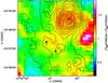 |
Fig. 4 Distribution of the line ratio of the 12CO(6–5) transition to the 12CO(3–2) line. Solid contours show the 12CO(6–5) integrated intensity in the velocity range vLSR = [−54, −40] km s-1 from 20% of the peak value in steps of 10%. The black triangles are as in Fig. 2. |
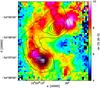 |
Fig. 5 Distribution of the second moment of the 12CO(6–5) line. The black solid contours represent the LABOCA continuum emission at 870 μm from 5% of the peak emission in steps of 5%. The peak of the continuum emission corresponds to the hot core position. |
Representative spectra of all 12CO transitions analysed in this study are presented in Fig. 6 towards the hot core, the IRDC position ((30′′, 30′′) from the centre of the APEX maps, see Sect. 4.2 and Figs. 2, 3) and the peak of the cm continuum emission in G327.3–0.5. Spectra of the 13CO transitions are shown in Fig. 7. Red- and blue-shifted wings are detected in the 12CO lines in a velocity range between −71 and −24 km s-1 (in 12CO(6–5)) towards G327.3–0.6 probably due to outflow motions. However, no sign of bipolar outflows is found when inspecting the integrated intensity maps of the blue- and red-shifted wings nor in position-velocity diagrams (Fig. 8). Moreover, very similar broad lines are detected along the whole extent of the infrared dark cloud, as shown in the top panel of Fig. 8. At the IRDC position, the wings in 12CO(6–5) range from −60 to −31 km s-1. All main isotopologue transitions analysed in this paper are affected by self-absorption (see Fig. 6 for reference spectra towards the hot core, the IRDC position and the Hii region); moreover, even the 13CO(6–5) line shows weak evidence of self-absorbed profile towards the hot core. Figure 9 shows the 12CO(7–6) spectra overlaid on the continuum emission at 870 μm: the self-reversed profile is spread over a large area and seems to follow the thermal dust continuum emission.
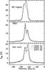 |
Fig. 6 Mean spectra over a beam of 18′′ (to match the resolution of the 12CO(3–2) data) of the 12CO isotopologue transitions analysed in the paper. The top panel shows spectra at the centre of G327.3–0.5, the middle panel spectra at the IRDC position, the bottom panel spectra at the hot core position. |
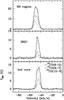 |
Fig. 7 Mean spectra over a beam of 21 |
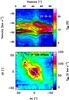 |
Fig. 8 Top panel: color scale and contours show the P − V diagram of the CO(6–5) transition computed along the cut indicated by the white arrow in the bottom panel. Offset positions increase along the direction of the arrow shown in the bottom panel. Bottom panel: distribution of the integrated intensity of the 13CO(6–5) transition towards the hot core G327.3–0.6. Solid contours show the continuum emission at 350 μm (Wyrowski et al., in prep.) from 3σ in steps of 10σ (σ ~ 3 Jy/beam). Symbols are as in Fig. 2. |
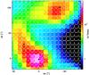 |
Fig. 9 Map of the 12CO(7–6) line overlaid on the continuum emission at 870 μm from LABOCA. The velocity axis ranges from −60 to −25 km s-1, the temperature axis from −1 to 15 K. The 12CO(7–6) data were smoothed to a resolution of 18″ to match the resolution of the 12CO(3–2) data and of the LABOCA emission. The centre of the map is that of the APEX data (see Sect. 2.1). The triangles and the green star are as in Fig. 2. |
Finally, the velocity field of the 12CO transitions may help us to understand the nature of the ring detected towards the Hii region G327.3–0.5. We therefore used the task KSHELL built in the visualisation software package KARMA (Gooch 1996). KSHELL computes an average brightness temperature on annuli about a user defined centre. A spherically symmetric expanding shell will look like a half ellipse in a (r − v) diagram with the axis in the v direction twice the expansion velocity. Figure 10 shows the resulting (r − v) diagram obtained with the 12CO(6–5) data cube using the peak of the cm continuum emission as centre. The emission does not follow a perfect spherical shell. This is likely due to inhomogeneities in the distribution of the gas, as already seen in Fig. 11 where the distribution of the optical depth of 13CO is not symmetric.
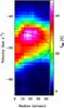 |
Fig. 10 (r − v) diagram of the Hii region G327.3–0.5 obtained from the 12CO(6–5) data cube. The radius axis is the distance to the shell expansion centre, chosen to be the peak of the cm continuum emission. The half ellipse represents an ideal shell in (r − v) diagram with an expansion velocity of 5 km s-1. |
4. Physical conditions of the warm gas
4.1. LTE analysis
From the line ratio of the 12CO(6–5) to 13CO(6–5) transitions we can derive the optical depth of the 12CO(6–5) line emission, which can be then used to infer the excitation temperature of the line and the column density of 12CO in the region.
The line intensity in a given velocity channel of a given transition is ![\begin{equation} \label{tl} T_{\rm{L}}=\eta\times\left[F_\nu\left(T_{\rm{ex}}\right)-F_\nu\left(T_{\rm{cbg}}\right)\right]\times\left(1-{\rm e}^{-\tau_\nu}\right) \end{equation}](/articles/aa/full_html/2013/02/aa18962-12/aa18962-12-eq44.png) (1)where η is the beam filling factor (assumed to be 1 in the following analysis), Fν = hν/k × [exp(hν/kT) − 1] -1, Tcbg = 2.7 K, and τν is the optical depth. Under the local thermodynamic equilibrium (LTE) assumption, Tex is assumed to be equal to the kinetic temperature of the gas and equal for all transitions. In the following analysis, we study the peak intensities of the 12CO(6–5) and 13CO(6–5) lines, and include only the cosmic background as background radiation and neglect, for example, any contribution from infrared dust emission since we do not have any map of the distribution of the dust temperature. This most likely affects only our estimates at the hot core position and possibly towards the Hii region G327.3–0.5 where SABOCA continuum emission at 350 μm is also detected (Wyrowski et al., in prep.). For an appropriate analysis of the emission from the hot core, see Rolffs et al. (2011).
(1)where η is the beam filling factor (assumed to be 1 in the following analysis), Fν = hν/k × [exp(hν/kT) − 1] -1, Tcbg = 2.7 K, and τν is the optical depth. Under the local thermodynamic equilibrium (LTE) assumption, Tex is assumed to be equal to the kinetic temperature of the gas and equal for all transitions. In the following analysis, we study the peak intensities of the 12CO(6–5) and 13CO(6–5) lines, and include only the cosmic background as background radiation and neglect, for example, any contribution from infrared dust emission since we do not have any map of the distribution of the dust temperature. This most likely affects only our estimates at the hot core position and possibly towards the Hii region G327.3–0.5 where SABOCA continuum emission at 350 μm is also detected (Wyrowski et al., in prep.). For an appropriate analysis of the emission from the hot core, see Rolffs et al. (2011).
Assuming that the 12CO(6–5) emission is optically thick and that the 12CO(6–5) and 13CO(6–5) lines have the same excitation temperatures, the optical depth of the 13CO(6–5) transition,  , is
, is  (2)The optical depth of the 12CO(6–5) transition can then be obtained by multiplying for the abundance of 12CO relative to 13CO, X12CO/13CO ~ 60 (Wilson & Rood 1994). From the optical depth of the 12CO(6–5) line, one can also derive its excitation temperature using Eq. (1). Figure 11 shows the distribution of the optical depth of the 13CO(6–5) line and of the excitation temperature of 12CO(6–5). The 13CO(6–5) emission is moderately optically thick (0.6–0.7) at the Hii region and at the infrared dark cloud, while it reaches values of ~1.2 at the hot core position and in a small part of ring around the Hii region. The map distribution of the excitation temperature of the 12CO(6–5) line is shown in the bottom panel of Fig. 11. The map is dominated by the Hii region, where Tex reaches values of 80 K in the ring around the Hii region and then decreases with increasing distance from it. The hot core and the rest of the infrared dark cloud have values around 30–35 K. The excitation temperature increases to the south west of the hot core, in a region where there is also 8 μm emission, and to the north-east of the Hii along a layer of gas also visible in the 12CO(6–5) integrated intensity map (see Fig. 2), but more prominent in the Tex map and in the 8 μm emission map (see Fig. 1).
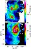 |
Fig. 11 Distribution of the optical depth of the 13CO(6–5) line ( |
From the optical depth and the excitation temperature of the 12CO(6–5) line, we derived the H2 column density assuming a relative abundance of 12CO relative to H2 of 2.7 × 10⁻⁴ (Lacy et al. 1994). Results are shown in Fig. 12. The largest column density is found towards the hot core (~3 × 1022 cm-2 in the 94 beam of the 13CO(6–5) data) and decreases along the infrared dark cloud with a distribution similar to that of the 870 μm continuum emission. Three peaks around 1022 cm-2 are found in the Hii region.
We cross-checked our results by computing the H2 column density under the assumption that the 13CO emission is optically thin. The results are consistent with those presented in Fig. 12; the largest differences (of the order of 30%) are found towards those positions where the optical depth of the 13CO(6–5) transition (Fig. 11) exceeds ~0.7. The assumption of optically thin emission for 13CO may be particularly useful for the inter-clump medium (arbitrarily defined as the region in the map where the 13CO lines are not detected on individual spectra), towards which we infer H2 column densities of ~2 × 1021 cm-2 corresponding to a 13CO column density of ~1016 cm-2 (see also Sect. 5.1).
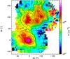 |
Fig. 12 Distribution of the H2 column density in the G327.3–0.6 star-forming region based on equation 1. Black contours are the 13CO(6–5) integrated intensity as in Fig. 3. |
We also computed column densities and rotational temperatures in the region using the rotational diagram technique applied to the 13CO data. We did not include the 12CO lines in the analysis because of their complex line profiles and high optical depths. Given the optical depth previously derived for the 13CO(6–5) line, we did not apply any correction due to optical depth effects to the 13CO data. Results are consistent with the estimates based on Eq. (1). The main differences between the two analyses are found towards the hot core, where the rotational temperature is higher than the excitation derived with Eq. (1) (Trot ~ 70 K and Tex ~ 32 K) and the H2 column density lower (1022 cm-2 versus 3 × 1022 cm-2 obtained with the first method). The differences between the two methods are likely influenced by the self-absorption profile detected in the 12CO(6–5) line which results in lower line intensities towards the regions of large column densities. In particular, while the first approach overestimates the optical depths (and hence column density) because of the self absorption, the column density derived with the rotational diagram analysis is likely underestimated towards the hot core because of the optically thin emission assumption, and should be corrected by a factor τLTE/(1−exp(τLTE)−) ~ 1.7.
Finally, we computed the ratio between the amount of warm gas (traced by 12CO and 13CO(6–5) and shown in Fig. 12) and the total amount of gas (traced by the continuum emission at 870 μm) as derived assuming a dust temperature equal to the excitation temperature of 12CO(6–5) and a dust opacity of 0.0182 cm2 g1 (Kauffmann et al. 2008). The results are shown in Fig. 13: the warm gas is only a small percentage (~10%) of the total gas in the infrared dark cloud, while it reaches values up to ~35% of the total gas in the ring surrounding the Hii region.
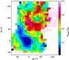 |
Fig. 13 Distribution of the ratio between the column density of warm gas (traced by 12CO and 13CO(6–5)) and the total H2 column density (traced by the continuum emission at 870 μm) in the G327.3–0.6 star-forming region. Black contours are the 13CO(6–5) integrated intensity as in Fig. 3. |
4.2. 13CO ladder
Since the G327.3–0.6 region was mapped in three different transitions of the 13CO molecule, we can perform a multi-line analysis towards selected positions and infer the parameter of the gas. The advantage of 13CO compared to the main isotopologue is in the lower opacities of the lines and in the less complex line profiles. For this analysis, we used the RADEX program (van der Tak et al. 2007) with expanding sphere geometry. The molecular dataset comes from the LAMDA database (Schöier et al. 2005) and includes collisional rates adapted from Yang et al. (2010). We ran models with temperatures from 20 to 200 K, densities in the range 104−5 × 107 cm-3, and 13CO column densities between 1014 and 1019 cm-2.
Line parameters of the 13CO lines.
All data were smoothed to the resolution of the 13CO(10–9) map. We selected three positions for the analysis: the hot core, the IRDC position ((30′′, 30′′) from the centre of the APEX maps), and the centre of the Hii region. The IRDC position was selected to be a position associated with high column density in the infrared dark cloud (see Figs. 2, 3 and 12) but without IR emission. However, it is only 10″ to the north of the EGO candidate (Cyganowski et al. 2008, see Figs. 2, 3), and therefore, given the beam of the observations, contamination from the embedded YSO may still be possible. Table 3 reports the measured line parameters of the 13CO transitions obtained with Gaussian fits; based on these values, we adopt line widths of 6, 3 and 7, for the hot core, the IRDC and the Hii respectively, in agreement with values reported by San José-García et al. (2012) for the 13CO(10–9) line towards a sample of intermediate- and high-mass sources. The spectra are shown in Fig. 7.
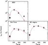 |
Fig. 14 Distribution of the 13CO peak line intensities. Full black triangles correspond to 13CO(6–5), (8–7) and (10–9) observed intensities. The circle represents the observed C18O(3–2) flux, the empty black triangle the flux of the C18O(3–2) line multiplied by X13CO/C18O ~ 8. The red triangles are the best model fit results. The error bars include only calibration uncertainties. The dashed lines represent the best fit 13CO ladder. |
Best fit parameters of the 13CO line modelling.
The results of the RADEX analysis are listed in Table 4 and shown in Fig. 14. For the IRDC position, the 13CO(10–9) line intensity is not well fitted by our one-temperature model. This likely reflects the fact that the 13CO(10–9) spectrum is dominated by the embedded source while the other two lines sample colder gas in the envelope. We considered a 20% calibration error for the 13CO(6–5) and (8–7) observations and a 15% error for the 13CO(10–9) data. Wyrowski et al. (2006) mapped the region with the APEX telescope in the C18O(3–2) line. Therefore, since no observations were performed in the 13CO(3–2) transition, we included the C18O(3–2) data in Fig. 14. Note however, that the C18O(3–2) fluxes are not included in the fitting procedure, but that they are simply used to cross-check results. Since the C18O(3–2) flux corresponds to a lower limit to the flux of 13CO(3–2) line, we also plotted the C18O(3–2) flux corrected for the abundance ratio of 13CO to C18O, X13CO/C18O ~ 8 (Wilson & Rood 1994). This value is likely an upper limit to the flux of the 13CO(3–2) line due to opacity effects.
An example of the χ2 distribution projected on to the T − n plane is shown in Fig. 15 for the Hii position, where the reduced χ2 at the best fit position is 3. Figure 15 shows the typical inverse n − T relationship often seen in χ2 distributions and due to the fact that density and temperature are, in the case of the CO molecule, not independent parameters (see Appendix C of van der Tak et al. 2007).
We note here that the detection of the 13CO(10–9) line breaks the degeneracy between density and temperature typical of 12CO analyses (e.g., Kramer et al. 2004; van der Tak et al. 2007) and help to give stronger constraints: indeed, with the exception of the hot core, at least the temperature of the gas is well determined at all positions.
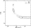 |
Fig. 15 Projection of the 3-dimensional (T-n-N) distribution of the χ2 on the T − n plane for the Hii position. The contours show the 1, 2 and 3σ confidence levels for two degrees of freedom. The triangle marks the best fit position. |
The results of the RADEX analysis confirm that the LTE assumption used in Sect. 4.1 is reasonable since the inferred densities are much larger than the critical densities (a few 104 cm-3 for all three analysed transitions). Assuming X12CO/13CO ~ 60 and an abundance of 12CO relative to H2 of 2.7 × 10⁻⁴, the derived 13CO column densities listed in Table 4 correspond to H2 column densities of some 1022 cm-2 for the hot core and the IRDC position, and of 2 × 1022 cm-2 for the Hii position. The derived column densities and temperatures are in agreement with those derived in Sect. 4.1 through rotational diagrams of the 13CO emission. The 13CO(6–5) optical depths are also in agreement with those estimated in Sect. 4.1 through the 13CO and 12CO(6–5) line ratio, with the exception of the hot core position: τLTE ~ 1.2 and τRADEX ~ 0.3 for the hot core, 0.6 and 0.5 for the Hii region, and 0.6 and 0.7 for the IRDC position.
We finally stress that the results obtained with the LTE analysis (Sect. 4.1) and with the RADEX code (this section) are based on the assumptions that 1) all lines have a beam filling factor of one, and 2) that the emitting gas is homogeneous, whereas self-absorption profiles in the 12CO lines indicate an excitation gradient along the line of sights. For optically thin lines (13CO in the current case), a beam filling factor less than one (but equal for all transitions) would mostly affect the column density and result in larger values of N; for optically thick lines, a smaller value of η would imply larger values of density and/or temperature.
The uncertainties on the derived parameters due to the assumption of a homogeneous medium are of less immediate interpretation, and more complex radiative transfer codes (e.g., Hogerheijde & van der Tak 2000) should be used to reproduce the observed line velocity profiles.
5. Discussion
5.1. Total 12CO and 13CO emission
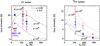 |
Fig. 16 CO (left) and 13CO (right) ladders for the whole mapped region (black), the Hii region G327.3–0.5 (red), the IRDC including the hot core (blue) and the inter-clump gas (magenta). Error bars include only calibration uncertainties. In both panels, the dashed and dotted curves represent the predicted intensities for model B from Koester et al. (1994) for a density of 107 cm-3, incident UV fields of 103 and 104 relative to the average interstellar field, a visual extinction of 10, and a Doppler broadening of 3 (dashed curve) and 1 km s-1 (dotted curve). |
Figure 16 shows the 12CO and 13CO ladders obtained by averaging the emission of the different observed transitions, smoothed to the resolution of the HIFI data, over four regions: the total map, the Hii region G327.3–0.5, the IRDC hosting the hot core (the selected region does include the hot core), and finally the inter-clump gas, which was defined as the region in the map where the 13CO lines are not detected on individual spectra. This region has an equivalent radius of 50′′(corresponding to ~0.8 pc at the distance of the source). Examples of 12CO line profiles towards the inter-clump gas are shown in Fig. 17. The C18O(3–2) cannot be used in this analysis because the observations cover a much smaller region than that mapped in 13CO. The total mass of the mapped region can be computed using the excitation temperature and H2 column density distributions shown in Figs. 11 and 12. This corresponds to ~700 M⊙.
Percentage of integrated fluxes from the Hii region G327.3–0.5 and from the inter-clump gas respect to the total integrated flux in the map.
The four regions have similar 12CO and 13CO ladders. In order to correct for self-absorption, integrated fluxes were obtained for each of the four regions from line fitting of the CO spectra with one Gaussian component. While this works fine for the spectra of the IRDC hosting the hot core and for the inter-clump gas, the line profiles of the total map and of Hii region are red-skewed and therefore the fluxes derived with this method are likely underestimated. For the main isotopologue, the flux of the (7–6) and (6–5) transitions is very similar, although for the IRDC + HC and the inter-clump the flux of the (7–6) line is lower than that of the (6–5) line. On the other hand, in the 13CO ladder the peak flux decreases with increasing energy level. For all transitions presented in this paper, the spectra are dominated in intensity by the Hii region, whose flux is of the order of 60% of the total flux for the main isotopologue lines, and ranging from ~49% of the total flux in the (6–5) line to ~85% in the (10–9) transition for 13CO (see Table 5). The main difference between the 12CO spectra and those of 13CO lies in the emission from the inter-clump gas: for all 12CO lines, the intensity is relatively strong, 10% of the flux from the whole region. On the other hand, the flux of the 13CO lines coming from the inter-clump gas decreases with increasing J, from ~7% of the total flux for J = 6 to ~2% for J = 10. The general behaviour of the 12CO and 13CO ladders is qualitatively compatible with PDR models from Koester et al. (1994) for high density (106−107 cm-3) clouds illuminated on one side by a UV radiation field (their model B). In Fig. 16, we show the predicted CO and 13CO line intensities for models with a density of 107 cm-3, incident UV fields with strength 103 and 104 relative to the average interstellar field (Draine 1978), a visual extinction of 10, and a Doppler broadening of 3 and 1 km s-1. High densities (n > 106 cm-3, in agreement with our results from Sect. 4.2) are needed to locate the peak of the CO ladders at mid-, high-J transitions (see Figs. 9–10, 12–13 of Koester et al. 1994). Stronger UV radiation fields also shift the peak of the CO ladders to higher J transitions than observed. In Fig. 16, the 12CO model intensities are corrected by a factor 0.2 and 0.25 to correct for different line-widths between the model and the observations, and possibly for beam dilution effects. On the other hand, the 13CO results of Fig. 16 are not scaled down by any factor as they are far too weak to match the observations.
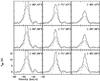 |
Fig. 17 CO(6–5) (solid line) and 12CO(7–6) (dashed line) spectra towards some positions in the inter-clump gas. The offset position from the centre of the APEX 12CO maps (Sect. 2.1) is shown for each spectrum in the top right corner. |
Koester et al. (1994) already noticed that the predicted line intensities of mid-J13CO transitions in their models are much weaker than observed in star-forming regions. They proposed that mid-J13CO emission comes from a large number of filamentary structures, or clumps, along the line of sight. In this way, the modelled line intensity of mid-J13CO lines would increase significantly as the lines are optically thin, while it would not change for optically thick transitions.
Rotational diagrams of the 13CO emission applied to the spectra of the Hii region, of the IRDC and of the inter-clump gas infer rotational temperatures of 66 K, 47 K and 44 K, respectively, and 13CO column densities of 6 × 1015 cm-2 for the Hii region and the IRDC, and of 2 × 1015 cm-2 for the inter-clump gas. Since the inter-clump gas has physical parameters very similar to those of the IRDC region, but a much lower column density, we suggest that it is composed of high-density clumps with low filling factors. This is again in agreement with PDR models (e.g., Koester et al. 1994; Cubick et al. 2008) which predict strong emission at mid-J13CO and high-J12CO lines in the case of small, low mass, high density clumps.
Cubick et al. (2008) suggested that the COBE 12CO ladder of the Milky Way can be reproduced by a clumpy PDR model, and that the bulk of the Galactic FIR line emission comes from PDRs around the Galactic population of massive stars. Our observations seem to confirm this result, since the CO emission of the G327.3–0.6 region is dominated by the PDR around the Hii region. Our results are also consistent with the findings from Davies et al. (2011) and Mottram et al. (2011). These authors studied the properties of massive YSOs and compact Hii regions in the RMS survey (Hoare et al. 2005), and found that there is no significant population of massive YSOs above ~105 L⊙, while compact Hii regions are detected up to ~106 L⊙. Since high-J CO lines are among the most important cooling lines in PDR, they reflect the luminosity of their heating sources: if the luminosity distribution of massive stars in the Galaxy is dominated by Hii regions and not by younger massive stars, then we also expect that the CO distribution follows the same rule.
5.2. Comparisons with other star forming regions
Large-scale mapping of some low- and high-mass star forming regions was performed in several 12CO transitions. However, given the different critical densities of the lines, we prefer to compare our results with studies carried on with J > 3 CO lines. Excitation temperatures around 8–30 K are found in extended diffuse emission and towards the brightest positions, respectively, in low-mass star forming regions (e.g., Davis et al. 2010; Curtis et al. 2010), while massive star-forming regions are usually warmer as confirmed by our findings (see also Wilson et al. 2001; Jakob et al. 2007; Kirk et al. 2010; Wilson et al. 2011; Peng et al. 2012). The CO column densities (1017–1018 cm-2 from the LTE analysis) found in G327 are also comparable with values obtained in other massive star-forming regions (Wilson et al. 2001; Jakob et al. 2007; White et al. 2010; Wilson et al. 2011).
Comparison with 12CO large maps of other high-mass star forming regions would be important to verify whether our result that the 12CO distribution is dominated by the Hii region is a common feature or not. However, most studies do not cover different evolutionary phases as in our case. For OMC-1, Peng et al. (2012) confirmed that the peak of the integrated intensity of several CO isotopologue lines is close to the Orion-KL hot core (although Orion-south and the Orion Bar PDR are also very prominent). One should notice however, that Orion is roughly six times closer to the Sun than G327.3–0.6, and therefore the Orion Bar and Orion-KL would be much closer on sky (~30″) if one would place them at the distance of G327.3–0.6. Moreover, Orion-KL likely represents a special case since it hosts a very powerful outflow (e.g., Kwan & Scoville 1976; Snell et al. 1984), which could alter the distribution of 12CO in the region. Indeed, Marrone et al. (2004) show that broad velocity emission arises mainly from the Orion-KL region, while much of the narrower emission arises from the PDR excited by the M42 Hii region.
5.3. Self-absorption profiles
As noted in Sect. 3.2, all 12CO transitions analysed in this paper are affected by self-absorption, which is likely to be due to cold gas surrounding a warmer component (Phillips et al. 1981). In particular along the infrared dark cloud (Fig. 8), the 12CO(6–5) line has blue-skewed profiles in the north-east (towards the EGO and the IRDC positions) and the red-skewed ones towards the south-west (the hot core). Blue- and red-skewed profiles (e.g., Mardones et al. 1997) are commonly interpreted as due to rotation or outflow motions (which should produce equal numbers of red and blue profiles, and could therefore explain the profiles detected towards the EGO and IRDC position, the hot core and the Hii region, Fig. 6) or to infall (which should produce profiles which are skewed towards the blue, e.g. towards the EGO and IRDC position) or to expansion (which should produce profiles skewed towards the red and could be responsible for the 12CO spectra of the hot core and the Hii region). From the PV diagram of the 12CO(6–5) line, we do not have any evidence of global rotation towards the hot core and the red-skewed profile can be interpreted in terms of expansion or outflow motion. Similarly, from Fig. 10 we see that the emission does not follow a perfect expanding spherical shell which might imply that the rotation is on the origin of the self-absorbed profile seen towards the Hii region. Finally, the blue-skewed line profile detected toward the EGO and IRDC positions are typical of infall motion.
6. Conclusions
To study the effect of feedback from massive star forming regions in their surrounding environment, we selected the region G327.3–0.6 for large scale mapping of several mid-J12CO and 13CO lines with the APEX telescope and of the high-J13CO(10–9) transition with the Herschel satellite. Our results can be summarised as follows:
-
1.
maps of all transitions are dominated by the PDR associatedwith the Hii region G327.3–0.5; mid-J12CO and 13CO emission is detected along the whole extent of the IRDC;
-
2.
mid-J transitions show rather extended emission with typical excitation temperatures of ~30 K and column densities of some 1021 cm-2;
-
3.
all observed transitions are detected also in the inter-clump gas when averaged over large regions. The inter-clump emission is compatible with LTE emission from a gas at 44 K, and with a 13CO column density of 2 × 1015 cm-2, thus suggesting that the inter-clump is composed of high-density clumps with low filling factors;
-
4.
the warm gas traced by 12 and 13CO(6–5) is only a small percentage (~10%) of the total gas in the infrared dark cloud, while it reaches values up to ~35% of the total gas in the ring surrounding the Hii region;
-
5.
the 12CO and 13CO ladders are qualitatively compatible with PDR models for high density gas (n > 106 cm-3) and, in the case of 13CO, suggest that the emission comes from a large number of clumps;
-
6.
the detection of the 13CO(10–9) line allows to give stronger constraints on the physics of the gas by breaking the degeneracy between density and temperature (typical of 12CO and 13CO transitions) in the high temperature-low density part of the T–n plane.
Acknowledgments
The authors thank Dr. Joe Mottram for a careful review of the manuscript and an anonymous referee for useful comments and suggestions. Herschel is an ESA space observatory with science instruments provided by European-led Principal Investigator consortia and with important participation from NASA. HIFI has been designed and built by a consortium of institutes and university departments from across Europe, Canada and the United States under the leadership of SRON Netherlands Institute for Space Research, Groningen, The Netherlands and with major contributions from Germany, France and the US. Consortium members are: Canada: CSA, U.Waterloo; France: CESR, LAB, LERMA, IRAM; Germany: KOSMA, MPIfR, MPS; Ireland, NUI Maynooth; Italy: ASI, IFSI-INAF, Osservatorio Astrofisico di Arcetri- INAF; Netherlands: SRON, TUD; Poland: CAMK, CBK; Spain: Observatorio Astronómico Nacional (IGN), Centro de Astrobiología (CSIC-INTA). Sweden: Chalmers University of Technology – MC2, RSS & GARD; Onsala Space Observatory; Swedish National Space Board, Stockholm University – Stockholm Observatory; Switzerland: ETH Zurich, FHNW; USA: Caltech, JPL, NHSC.
References
- Beuther, H., Schilke, P., Sridharan, T. K., et al. 2002, A&A, 383, 892 [NASA ADS] [CrossRef] [EDP Sciences] [Google Scholar]
- Blitz, L., & Stark, A. A. 1986, ApJ, 300, L89 [NASA ADS] [CrossRef] [Google Scholar]
- Cubick, M., Stutzki, J., Ossenkopf, V., Kramer, C., & Röllig, M. 2008, A&A, 488, 623 [NASA ADS] [CrossRef] [EDP Sciences] [Google Scholar]
- Curtis, E. I., Richer, J. S., & Buckle, J. V. 2010, MNRAS, 401, 455 [NASA ADS] [CrossRef] [Google Scholar]
- Cyganowski, C. J., Whitney, B. A., Holden, E., et al. 2008, AJ, 136, 2391 [NASA ADS] [CrossRef] [Google Scholar]
- Davies, B., Hoare, M. G., Lumsden, S. L., et al. 2011, MNRAS, 1015 [Google Scholar]
- Davis, C. J., Chrysostomou, A., Hatchell, J., et al. 2010, MNRAS, 405, 759 [NASA ADS] [Google Scholar]
- de Graauw, T., Helmich, F. P., Phillips, T. G., et al. 2010, A&A, 518, L6 [NASA ADS] [CrossRef] [EDP Sciences] [Google Scholar]
- Draine, B. T. 1978, ApJS, 36, 595 [NASA ADS] [CrossRef] [Google Scholar]
- Gibb, E., Nummelin, A., Irvine, W. M., Whittet, D. C. B., & Bergman, P. 2000, ApJ, 545, 309 [NASA ADS] [CrossRef] [PubMed] [Google Scholar]
- Gooch, R. 1996, in Astronomical Data Analysis Software and Systems V, eds. G. H. Jacoby, & J. Barnes, ASP Conf. Ser., 101, 80 [Google Scholar]
- Goss, W. M., & Shaver, P. A. 1970, Aust. J. Phys. Astrophys. Suppl., 14, 1 [Google Scholar]
- Güsten, R., Baryshev, A., Bell, A., et al. 2008, in SPIE Conf. Ser. 7020 [Google Scholar]
- Hoare, M. G., Lumsden, S. L., Oudmaijer, R. D., et al. 2005, in Massive Star Birth: A Crossroads of Astrophysics, eds. R. Cesaroni, M. Felli, E. Churchwell, & M. Walmsley, IAU Symp., 227, 370 [Google Scholar]
- Hogerheijde, M. R. & van der Tak, F. F. S. 2000, A&A, 362, 697 [NASA ADS] [Google Scholar]
- Jakob, H., Kramer, C., Simon, R., et al. 2007, A&A, 461, 999 [NASA ADS] [CrossRef] [EDP Sciences] [Google Scholar]
- Kasemann, C., Güsten, R., Heyminck, S., et al. 2006, in SPIE Conf. Ser. 6275 [Google Scholar]
- Kauffmann, J., Bertoldi, F., Bourke, T. L., Evans, II, N. J., & Lee, C. W. 2008, A&A, 487, 993 [NASA ADS] [CrossRef] [EDP Sciences] [Google Scholar]
- Kirk, J. M., Polehampton, E., Anderson, L. D., et al. 2010, A&A, 518, L82 [NASA ADS] [CrossRef] [EDP Sciences] [Google Scholar]
- Klein, B., Philipp, S. D., Krämer, I., et al. 2006, A&A, 454, L29 [NASA ADS] [CrossRef] [EDP Sciences] [Google Scholar]
- Koester, B., Stoerzer, H., Stutzki, J., & Sternberg, A. 1994, A&A, 284, 545 [NASA ADS] [Google Scholar]
- Kramer, C., Jakob, H., Mookerjea, B., et al. 2004, A&A, 424, 887 [NASA ADS] [CrossRef] [EDP Sciences] [Google Scholar]
- Kwan, J., & Scoville, N. 1976, ApJ, 210, L39 [NASA ADS] [CrossRef] [Google Scholar]
- Lacy, J. H., Knacke, R., Geballe, T. R., & Tokunaga, A. T. 1994, ApJ, 428, L69 [NASA ADS] [CrossRef] [Google Scholar]
- Mardones, D., Myers, P. C., Tafalla, M., et al. 1997, ApJ, 489, 719 [NASA ADS] [CrossRef] [Google Scholar]
- Marrone, D. P., Battat, J., Bensch, F., et al. 2004, ApJ, 612, 940 [NASA ADS] [CrossRef] [Google Scholar]
- Minier, V., André, P., Bergman, P., et al. 2009, A&A, 501, L1 [NASA ADS] [CrossRef] [EDP Sciences] [Google Scholar]
- Moisés, A. P., Damineli, A., Figuerêdo, E., et al. 2011, MNRAS, 411, 705 [NASA ADS] [CrossRef] [Google Scholar]
- Mottram, J. C., Hoare, M. G., Davies, B., et al. 2011, ApJ, 730, L33 [NASA ADS] [CrossRef] [Google Scholar]
- Ott, S. 2010, in Astronomical Data Analysis Software and Systems XIX, eds. Y. Mizumoto, K.-I. Morita, & M. Ohishi, ASP Conf. Ser., 434, 139 [Google Scholar]
- Peng, T.-C., Wyrowski, F., Zapata, L. A., Güsten, R., & Menten, K. M. 2012, A&A, accepted [Google Scholar]
- Phillips, T. G., Knapp, G. R., Wannier, P. G., et al. 1981, ApJ, 245, 512 [NASA ADS] [CrossRef] [Google Scholar]
- Pilbratt, G. L., Riedinger, J. R., Passvogel, T., et al. 2010, A&A, 518, L1 [CrossRef] [EDP Sciences] [Google Scholar]
- Roelfsema, P. R., Helmich, F. P., Teyssier, D., et al. 2012, A&A, 537, A17 [NASA ADS] [CrossRef] [EDP Sciences] [Google Scholar]
- Rolffs, R., Schilke, P., Wyrowski, F., et al. 2011, A&A, 527, A68 [NASA ADS] [CrossRef] [EDP Sciences] [Google Scholar]
- San José-García, I., Mottram, J. C., Kristensen, L. E., et al. 2012, A&A, submitted [Google Scholar]
- Schöier, F. L., van der Tak, F. F. S., van Dishoeck, E. F., & Black, J. H. 2005, A&A, 432, 369 [NASA ADS] [CrossRef] [EDP Sciences] [Google Scholar]
- Schuller, F., Menten, K. M., Contreras, Y., et al. 2009, A&A, 504, 415 [NASA ADS] [CrossRef] [EDP Sciences] [Google Scholar]
- Snell, R. L., Scoville, N. Z., Sanders, D. B., & Erickson, N. R. 1984, ApJ, 284, 176 [NASA ADS] [CrossRef] [Google Scholar]
- Stutzki, J., & Güsten, R. 1990, ApJ, 356, 513 [NASA ADS] [CrossRef] [Google Scholar]
- Urquhart, J. S., Hoare, M. G., Lumsden, S. L., et al. 2011, MNRAS, 2112 [Google Scholar]
- van der Tak, F. F. S., Black, J. H., Schöier, F. L., Jansen, D. J., & van Dishoeck, E. F. 2007, A&A, 468, 627 [NASA ADS] [CrossRef] [EDP Sciences] [Google Scholar]
- van Dishoeck, E. F., Kristensen, L. E., Benz, A. O., et al. 2011, PASP, 123, 138 [NASA ADS] [CrossRef] [Google Scholar]
- White, G. J., Abergel, A., Spencer, L., et al. 2010, A&A, 518, L114 [NASA ADS] [CrossRef] [EDP Sciences] [Google Scholar]
- Wilson, T. L., & Rood, R. 1994, ARA&A, 32, 191 [NASA ADS] [CrossRef] [Google Scholar]
- Wilson, T. L., Muders, D., Kramer, C., & Henkel, C. 2001, ApJ, 557, 240 [NASA ADS] [CrossRef] [Google Scholar]
- Wilson, T. L., Muders, D., Dumke, M., Henkel, C., & Kawamura, J. H. 2011, ApJ, 728, 61 [NASA ADS] [CrossRef] [Google Scholar]
- Wyrowski, F., Menten, K. M., Schilke, P., et al. 2006, A&A, 454, L91 [NASA ADS] [CrossRef] [EDP Sciences] [Google Scholar]
- Wyrowski, F., Bergman, P., Menten, K., et al. 2008, Ap&SS, 313, 69 [NASA ADS] [CrossRef] [Google Scholar]
- Yang, B., Stancil, P. C., Balakrishnan, N., & Forrey, R. C. 2010, ApJ, 718, 1062 [NASA ADS] [CrossRef] [Google Scholar]
All Tables
Percentage of integrated fluxes from the Hii region G327.3–0.5 and from the inter-clump gas respect to the total integrated flux in the map.
All Figures
|
Fig. 1 Spitzer infrared colour image of the region G327.3–0.6 with red representing 8.0 μm, green 4.5 μm and blue 3.6 μm. The blue contours represent the integrated intensity of the 12CO(6–5) line (thin contours are 15%, 45% and 70% of the peak emission, thick contours 30%, 60% and 90% of the peak emission). The sources discussed in this paper (the IRDC, the EGO, the hot core G327.3–0.6, the SMM6 position and the Hii region G327.3–0.5) are also marked with crosses. The white and yellow boxes mark the regions mapped with APEX and Herschel, respectively. |
| In the text | |
|
Fig. 2 Maps of the integrated intensity of the 12CO(3–2), (6–5) and (7–6) lines in the velocity range vLSR = [−54, −40] km s-1 (color scale). Solid contours are the integrated intensity of the 12CO(6–5) line from 20% of the peak emission in steps of 10%. In each panel, the positions analysed in Sect. 4.2 (the hot core, the IRDC position, and the centre of the Hii region) are marked with black triangles. The red star labels the position of the EGO. SMM6 (left panel) is one of the submillimetre sources detected by Minier et al. (2009). |
| In the text | |
|
Fig. 3 Maps of the integrated intensity of the 13CO(6–5), (8–7) and (10–9) transitions in the velocity range vLSR = [−54, −40] km s-1 (colour scale). The solid contours in the left panel represent the LABOCA continuum emission at 870 μm from 5% of the peak emission in steps of 10% (Schuller et al. 2009). In the middle and right panels, the solid contours are the integrated intensity of the 13CO(6–5) from 20% of the peak emission in steps of 10%. In each panel, the positions analysed in Sect. 4.2 (the hot core, the IRDC position, and the centre of the Hii region) are marked with black triangles (except in the left panel, where the hot core is shown by a white triangle). The red star labels the position of the EGO. |
| In the text | |
|
Fig. 4 Distribution of the line ratio of the 12CO(6–5) transition to the 12CO(3–2) line. Solid contours show the 12CO(6–5) integrated intensity in the velocity range vLSR = [−54, −40] km s-1 from 20% of the peak value in steps of 10%. The black triangles are as in Fig. 2. |
| In the text | |
|
Fig. 5 Distribution of the second moment of the 12CO(6–5) line. The black solid contours represent the LABOCA continuum emission at 870 μm from 5% of the peak emission in steps of 5%. The peak of the continuum emission corresponds to the hot core position. |
| In the text | |
|
Fig. 6 Mean spectra over a beam of 18′′ (to match the resolution of the 12CO(3–2) data) of the 12CO isotopologue transitions analysed in the paper. The top panel shows spectra at the centre of G327.3–0.5, the middle panel spectra at the IRDC position, the bottom panel spectra at the hot core position. |
| In the text | |
|
Fig. 7 Mean spectra over a beam of 21 |
| In the text | |
|
Fig. 8 Top panel: color scale and contours show the P − V diagram of the CO(6–5) transition computed along the cut indicated by the white arrow in the bottom panel. Offset positions increase along the direction of the arrow shown in the bottom panel. Bottom panel: distribution of the integrated intensity of the 13CO(6–5) transition towards the hot core G327.3–0.6. Solid contours show the continuum emission at 350 μm (Wyrowski et al., in prep.) from 3σ in steps of 10σ (σ ~ 3 Jy/beam). Symbols are as in Fig. 2. |
| In the text | |
|
Fig. 9 Map of the 12CO(7–6) line overlaid on the continuum emission at 870 μm from LABOCA. The velocity axis ranges from −60 to −25 km s-1, the temperature axis from −1 to 15 K. The 12CO(7–6) data were smoothed to a resolution of 18″ to match the resolution of the 12CO(3–2) data and of the LABOCA emission. The centre of the map is that of the APEX data (see Sect. 2.1). The triangles and the green star are as in Fig. 2. |
| In the text | |
|
Fig. 10 (r − v) diagram of the Hii region G327.3–0.5 obtained from the 12CO(6–5) data cube. The radius axis is the distance to the shell expansion centre, chosen to be the peak of the cm continuum emission. The half ellipse represents an ideal shell in (r − v) diagram with an expansion velocity of 5 km s-1. |
| In the text | |
|
Fig. 11 Distribution of the optical depth of the 13CO(6–5) line ( |
| In the text | |
|
Fig. 12 Distribution of the H2 column density in the G327.3–0.6 star-forming region based on equation 1. Black contours are the 13CO(6–5) integrated intensity as in Fig. 3. |
| In the text | |
|
Fig. 13 Distribution of the ratio between the column density of warm gas (traced by 12CO and 13CO(6–5)) and the total H2 column density (traced by the continuum emission at 870 μm) in the G327.3–0.6 star-forming region. Black contours are the 13CO(6–5) integrated intensity as in Fig. 3. |
| In the text | |
|
Fig. 14 Distribution of the 13CO peak line intensities. Full black triangles correspond to 13CO(6–5), (8–7) and (10–9) observed intensities. The circle represents the observed C18O(3–2) flux, the empty black triangle the flux of the C18O(3–2) line multiplied by X13CO/C18O ~ 8. The red triangles are the best model fit results. The error bars include only calibration uncertainties. The dashed lines represent the best fit 13CO ladder. |
| In the text | |
|
Fig. 15 Projection of the 3-dimensional (T-n-N) distribution of the χ2 on the T − n plane for the Hii position. The contours show the 1, 2 and 3σ confidence levels for two degrees of freedom. The triangle marks the best fit position. |
| In the text | |
|
Fig. 16 CO (left) and 13CO (right) ladders for the whole mapped region (black), the Hii region G327.3–0.5 (red), the IRDC including the hot core (blue) and the inter-clump gas (magenta). Error bars include only calibration uncertainties. In both panels, the dashed and dotted curves represent the predicted intensities for model B from Koester et al. (1994) for a density of 107 cm-3, incident UV fields of 103 and 104 relative to the average interstellar field, a visual extinction of 10, and a Doppler broadening of 3 (dashed curve) and 1 km s-1 (dotted curve). |
| In the text | |
|
Fig. 17 CO(6–5) (solid line) and 12CO(7–6) (dashed line) spectra towards some positions in the inter-clump gas. The offset position from the centre of the APEX 12CO maps (Sect. 2.1) is shown for each spectrum in the top right corner. |
| In the text | |
Current usage metrics show cumulative count of Article Views (full-text article views including HTML views, PDF and ePub downloads, according to the available data) and Abstracts Views on Vision4Press platform.
Data correspond to usage on the plateform after 2015. The current usage metrics is available 48-96 hours after online publication and is updated daily on week days.
Initial download of the metrics may take a while.