| Issue |
A&A
Volume 548, December 2012
|
|
|---|---|---|
| Article Number | A66 | |
| Number of page(s) | 28 | |
| Section | Catalogs and data | |
| DOI | https://doi.org/10.1051/0004-6361/201220142 | |
| Published online | 22 November 2012 | |
The Sloan Digital Sky Survey quasar catalog: ninth data release⋆
1
UPMC-CNRS, UMR 7095, Institut d’Astrophysique de Paris,
75014
Paris,
France
e-mail: This email address is being protected from spambots. You need JavaScript enabled to view it.
2
Departamento de Astronomía, Universidad de Chile,
Casilla 36-D, Santiago, Chile
3
APC, Astroparticule et Cosmologie, Université Paris Diderot,
CNRS/IN2P3, CEA/Irfu, Observatoire de Paris, Sorbonne Paris Cité, 10 rue Alice Domon & Léonie
Duquet, 75205
Paris Cedex 13,
France
4
Lawrence Berkeley National Lab, 1 Cyclotron Rd,
Berkeley
CA, 94720, USA
5
Department of Physics and Astronomy, University of
Wyoming, Laramie,
WY
82071,
USA
6
Max-Planck-Institut für Astronomie, Königstuhl 17, 69117
Heidelberg,
Germany
7
Princeton University Observatory, Peyton Hall, Princeton, NJ
08544,
USA
8
University of Washington, Dept. of Astronomy, Box 351580, Seattle, WA
98195,
USA
9
Institut de Ciències del Cosmos (IEEC/UB),
Barcelona,
Catalonia,
Spain
10
Apache Point Observatory, PO Box 59, Sunspot, NM
88349-0059,
USA
11 Department of Physics and Astronomy, University of Utah,
UT, USA
12
Institute for Advanced Study, Einstein Drive, Princeton, NJ
08540,
USA
13
Department of Astronomy and Astrophysics, The Pennsylvania State
University, University
Park, PA
16802,
USA
14
Institute for Gravitation and the Cosmos, The Pennsylvania State
University, University
Park, PA
16802,
USA
15
Department of Astronomy, University of Florida,
Gainesville, FL
32611-2055,
USA
16
School of Physics and Astronomy, Tel Aviv University,
Tel Aviv
69978,
Israel
17
Carnegie Mellon University, Physics Department,
5000 Forbes Ave, Pittsburgh, PA
15213,
USA
18
CEA, Centre de
Saclay, Irfu/SPP, 91191
Gif-sur-Yvette,
France
19
Harvard-Smithsonian Center for Astrophysics, 60 Garden St., MS#20,
Cambridge,
MA
02138,
USA
20 Department of Astronomy, Yale University, New Haven,
CT06511, USA
21
Steward Observatory, University of Arizona,
933 North Cherry
Avenue, Tucson,
AZ
85721,
USA
22
Faculty of Sciences, Department of Astronomy and Space Sciences,
Erciyes University, 38039
Kayseri,
Turkey
23
Institute of Theoretical Physics, University of Zurich,
8057
Zurich,
Switzerland
24 Department of Physics and Astronomy, York University,
Toronto, ON M3J1P3, Canada
25
Center for Cosmology and Particle Physics, Department of Physics,
New York University, 4 Washington
Place, New York,
NY
10003,
USA
26
National Radio Astronomy Observatory, 520 Edgemont Rd., Charlottesville, VA
22903,
USA
27
Department of Physics and Astronomy, UC Irvine, 4129 Frederick Reines Hall,
Irvine, CA
92697-4575,
USA
28 Department of Astrophysical sciences, Princeton university,
Princeton 08544, USA
29
Institute of Cosmology and Gravitation, University of Portsmouth,
Dennis Sciama
building, Portsmouth
P01 3FX,
UK
30
Institute of Astronomy, University of Cambridge,
Madingley Road,
Cambridge
CB3 0HA,
UK
31
Institució Catalana de Recerca i Estudis Avançats,
Catalonia,
Spain
32
Center for Cosmology and Particle Physics, Department of Physics,
New York University, New
York, NY
10003,
USA
33
Instituto de Astrofísica de Canarias (IAC),
38200
La Laguna, Tenerife,
Spain
34
Departamento de Astrofisica, Universidad de La Laguna
(ULL), 38205 La
Laguna, Tenerife,
Spain
35
Department of Physics, Drexel University,
Philadelphia, PA
19104,
USA
36
5 Brookhaven National Laboratory, Blgd 510, Upton, NY
11375,
USA
37
Department of Physics, University of California
Berkeley, Berkeley,
CA
94720,
USA
38
INAF – Osservatorio Astronomico di Trieste, via G.B. Tiepolo 11,
Trieste,
Italy
39
INFN/National Institute for Nuclear Physics,
via Valerio 2,
34127
Trieste,
Italy
40
Astronomy Department and Center for Cosmology and AstroParticle
Physics, Ohio State University, 140
West 18th Avenue, Columbus, OH
43210,
USA
41
PITT PACC, Department of Physics and Astronomy, University of
Pittsburgh, Pittsburgh, PA
15260,
USA
Received: 31 July 2012
Accepted: 7 October 2012
Abstract
We present the Data Release 9 Quasar (DR9Q) catalog from the Baryon Oscillation Spectroscopic Survey (BOSS) of the Sloan Digital Sky Survey III. The catalog includes all BOSS objects that were targeted as quasar candidates during the survey, are spectrocopically confirmed as quasars via visual inspection, have luminosities Mi[z = 2] < −20.5 (in a ΛCDM cosmology with H0 = 70 km s-1 Mpc-1, ΩM = 0.3, and ΩΛ = 0.7) and either display at least one emission line with full width at half maximum (FWHM) larger than 500 km s-1 or, if not, have interesting/complex absorption features. It includes as well, known quasars (mostly from SDSS-I and II) that were reobserved by BOSS. This catalog contains 87 822 quasars (78 086 are new discoveries) detected over 3275 deg2 with robust identification and redshift measured by a combination of principal component eigenspectra newly derived from a training set of 8632 spectra from SDSS-DR7. The number of quasars with z > 2.15 (61 931) is ~2.8 times larger than the number of z > 2.15 quasars previously known. Redshifts and FWHMs are provided for the strongest emission lines (C iv, C iii], Mg ii). The catalog identifies 7533 broad absorption line quasars and gives their characteristics. For each object the catalog presents five-band (u, g, r, i, z) CCD-based photometry with typical accuracy of 0.03 mag, and information on the morphology and selection method. The catalog also contains X-ray, ultraviolet, near-infrared, and radio emission properties of the quasars, when available, from other large-area surveys. The calibrated digital spectra cover the wavelength region 3600−10 500 Å at a spectral resolution in the range 1300 < R < 2500; the spectra can be retrieved from the SDSS Catalog Archive Server. We also provide a supplemental list of an additional 949 quasars that have been identified, among galaxy targets of the BOSS or among quasar targets after DR9 was frozen.
Key words: catalogs / surveys / quasars: general
Catalog is only available at the CDS via anonymous ftp to cdsarc.u-strasbg.fr (130.79.128.5) or via http://cdsarc.u-strasbg.fr/viz-bin/qcat?J/A+A/548/A66
Hubble fellow.
© ESO, 2012
1. Introduction
Since their discovery (Schmidt 1963), interest in quasars has grown steadily, both because of their peculiar properties and because of their importance for cosmology and galaxy evolution. Many catalogs have gathered together increasing numbers of quasars either from heterogeneous samples (see Hewitt & Burbidge 1993; Véron-Cetty & Véron 2006,and references therein) or from large surveys, most importantly: the Large Bright Quasar Survey (LBQS, Morris et al. 1991; Hewett et al. 1995); the 2dF Quasar Redshift Survey (2QZ; Boyle et al. 2000; Croom et al. 2001) and the successive releases of the Sloan Digital Sky Survey (SDSS, York et al. 2000) Quasar Catalogs (e.g., Schneider et al. 2010,for DR7).
This paper describes the first quasar catalog of the Baryon Oscillation Spectroscopic Survey (BOSS, Schlegel et al. 2007; Dawson et al. 2012). BOSS is the main dark time legacy survey of the third stage of the Sloan Digital Sky Survey (SDSS-III, Eisenstein et al. 2011). It is based on the ninth data release of the SDSS (Ahn et al. 2012). BOSS is a five-year program to obtain spectra of 1.5 million of galaxies and over 150 000 z > 2.15 quasars. The main goal of the survey is to detect the characteristic scale imprinted by baryon acoustic oscillations (BAO) in the early universe from the spatial distribution of both luminous red galaxies at z ~ 0.7 and H i absorption lines in the intergalactic medium (IGM) at z ~ 2.5. BOSS uses the same imaging data as in SDSS-I and II, with an extension in the south Galactic cap (SGC).
The BAO clustering measurements in the IGM require a quasar catalog of maximal purity and accurate redshifts. Indeed the spectra of any non-quasar object, especially at high signal-to-noise ratio, will dilute the signal and/or increase the noise in the clustering measurement. The automated processing of the spectra (Bolton et al. 2012) is sophisticated, but is not perfect. The identification of the objects and their redshifts have therefore to be certified before any analysis is performed. The present catalog, henceforth denoted DR9Q catalog, contains 87 822 quasars identified among the objects targeted as quasar candidates over an area of 3275 deg2 surveyed during the first two years of BOSS operations. We also give a supplemental list of quasars identified among galaxy targets. This catalog keeps the tradition of producing quasar catalogs (Schneider et al. 2002, 2003, 2005, 2007, 2010) from SDSS-I and II (York et al. 2000). The final version of the SDSS-II quasar catalog (Schneider et al. 2010) based on the seventh SDSS data release (Abazajian et al. 2009) contains 105 783 objects mostly at z < 2 (see Shen et al. 2011,for their properties). Note that the DR9Q catalog does not contain all DR7 quasars but only those DR7 quasars that were reobserved during the two first years of BOSS1. High redshift (z > 2) quasar continua together with pixel masks, improved noise estimates, and other products designed to aid in the BAO-Lyman-α clustering analysis will be released in Lee et al. (in prep.).
The selection of candidates and observations are summarized in Sect. 2. We describe the visual inspection of all targets in Sect. 3, present accurate redshifts for the quasars in Sect. 4 and describe the detection and measurement of broad absorption lines (BALs) in Sect. 5. The catalog is described in Sect. 6. We give a catalog summary in Sect. 7 and comment on the supplemental lists of quasars in Sect. 8. We conclude in Sect. 9.
In the following we will use a ΛCDM cosmology with H0 = 70 km s-1 Mpc-1, ΩM = 0.3, and ΩΛ = 0.7 (Spergel et al. 2003).
Most of the objects in the catalog show at least an emission line with FWHM > 500 km s-1 in their spectra. However, there are a few exceptions: a few objects have emission lines with smaller FWHM due to noise or dust obscuration (Type II quasars) others have very weak emission lines but are identified as quasars because of the presence of the Lyman-α forest (Diamond-Stanic et al. 2009). We will call a quasar an object with a luminosity Mi[z = 2] < −20.5 and either displaying at least one emission line with FWHM greater than 500 km s-1 or, if not, having interesting/complex absorption features. This definition is slightly different from the one used in SDSS-DR7. The change in absolute magnitude is to include a few low-z objects in the catalog. Because BOSS is targeting z > 2.15 quasars, the median absolute luminosity is higher in BOSS than in SDSS-DR7. All BOSS objects with z > 2 qualify for the SDSS-DR7 definition: FWHM > 1000 km s-1 and Mi[z = 0] < −22 (adopting the same cosmology and αν = −0.5). In the following, all magnitudes will be PSF magnitudes.
2. Survey outline
In order to measure the BAO scale in the Lyman-α forest at z ~ 2.5, BOSS aims to obtain spectra of over 150 000 quasars in the redshift range 2.15 ≤ z ≤ 3.5, where at least part of the Lyman-α forest lies in the BOSS spectral range. The measurement of clustering in the IGM is independent of the properties of background quasars. Therefore the quasar sample does not need to be uniform and a variety of selection methods are used to increase the surface density of high redshift quasars (Ross et al. 2012). Some quasars with z < 2 will be targeted in the course of specific ancillary science programs or as a consequence of imperfect high-redshift quasar selection.
To detect the BAO signal, a surface density of 15 quasars with z ≥ 2.15 per square degree is required (McDonald & Eisenstein 2007). For comparison, SDSS-I/II targeted about ~14 000 z ≥ 2.15 quasars over the full survey, e.g. ~8400 deg2 (Schneider et al. 2010), leading to a surface density of ~2 quasars per square degree in the redshift range of interest for BOSS. To reach the BAO quasar density requirement implies targeting to fainter magnitudes than SDSS-I/II. The BOSS limiting magnitude for target selection is r ≤ 21.85 or g ≤ 22 (Ross et al. 2012), while z ≥ 3 quasars were selected to be brighter than i ~ 20.2 in SDSS-I/II (Richards et al. 2002).
2.1. Imaging data
BOSS uses the same imaging data as that of the original SDSS-I/II survey, with an extension in the SGC. These data were gathered using a dedicated 2.5 m wide-field telescope (Gunn et al. 2006) to collect light for a camera with 30 2k × 2k CCDs (Gunn et al. 1998) over five broad bands – ugriz (Fukugita et al. 1996); this camera has imaged 14 555 unique square degrees of the sky, including ~7500 deg2 in the NGC and ~3100 deg2 in the SGC (Aihara et al. 2011). The imaging data were taken on dark photometric nights of good seeing (Hogg et al. 2001). Objects were detected and their properties were measured (Lupton et al. 2001; Stoughton et al. 2002) and calibrated photometrically (Smith et al. 2002; Ivezić et al. 2004; Tucker et al. 2006; Padmanabhan et al. 2008), and astrometrically (Pier et al. 2003).
2.2. Target selection
The target selection of quasar candidates is crucial for the goals of the quasar BOSS survey. On average 40 fibers per square degree are allocated by the survey to the quasar project. The surface density of z ≥ 2.15 quasars to the BOSS magnitude limit is approximately 28 per deg2 (see Palanque-Delabrouille et al. 2012). Thus, recovering these quasars from 40 targets per square degree in single-epoch SDSS imaging is challenging because photometric errors are significant at this depth and because the quasar locus (in ugriz) crosses the stellar locus at z ~ 2.7 (Fan 1999; Richards et al. 2002; Ross et al. 2012). All objects classified as point-sources in the imaging data and brighter than either r = 21.85 or g = 22 (or both, magnitudes dereddened for Galactic extinction) are passed through the various quasar target selection algorithms. The quasar target selection for the first two years of BOSS operation is fully described in Ross et al. (2012). We briefly summarize here the key steps.
The target selection algorithm is designed to maximize the number of quasars useful for the Lyman-α forest analyses and reach the requirement of 15 deg-2 quasars with z ≥ 2.15. Several target selection methods are therefore combined and data in other wavelength bands are used when available. At the same time, in order to use the quasars themselves for statistical studies, such as the quasar luminosity function or clustering analyses (e.g. White et al. 2012), part of the sample must be uniformly selected. Thus, the BOSS quasar target selection is split in two parts:
-
About half of the targets are selected as part of the so-called“CORE” sample using a single uniform target selectionalgorithm. The likelihood method (Kirkpatricket al. 2011) was adopted for theCORE selection during the first year ofobservations. Starting with the second year of operation,it was replaced by the extreme deconvolutionmethod (XDQSO; Bovyet al. 2011) which better takesphotometric errors into account.
-
Most of the remaining quasar candidates are selected as part of the so-called “BONUS” sample through a combination of four methods: the non-parametric Bayesian classification and kernel density estimator (KDE; Richards et al. 2004, 2009), the likelihood method (Kirkpatrick et al. 2011), a neural network (Yèche et al. 2010) and the XDQSO method (Bovy et al. 2011, 2012, objects for lower likelihood than in the CORE sample, over a slightly expanded redshift range, and incorporating data from UKIDSS; Lawrence et al. (2007); from GALEX; Martin et al. (2005); and, where available, from coadded imaging in overlapping SDSS runs). The outputs of all of these BONUS methods are combined using a neural network.
Point-sources that match FIRST (Becker et al. 1995) and that are not blue in u − g (which would be characteristic of z < 2 quasars) are also always included. In addition, previously known z > 2.15 quasars (mostly from SDSS I/II) were also re-targeted for several reasons: (i) the BOSS wavelength range is more extended than in previous surveys; (ii) BOSS spectra have usually higher signal-to-noise ratio (S/N) than SDSS spectra (Ahn et al. 2012); (iii) the two epoch data will allow spectral variability studies. This sample is selected using the SDSS-DR7 quasar catalog (Schneider et al. 2010), the 2dF QSO Redshift Survey (2QZ; Croom et al. 2004), the 2dF-SDSS LRG and QSO Survey (2SLAQ; Croom et al. 2009), the AAT-UKIDSS-SDSS (AUS) survey, and the MMT-BOSS pilot survey (Appendix C in Ross et al. 2012). Quasars observed at high spectral resolution by UVES-VLT and HIRES-Keck were also included in the sample. Finally, BOSS includes targeting of a number of ancillary programs, some designed specifically to target quasars (e.g., the variability programs; Palanque-Delabrouille et al. 2011; MacLeod et al. 2012). The corresponding programs include:
-
Reddened quasars: quasar candidates with high intrinsicreddening.
-
No quasar left behind: bright variable quasars on Stripe 82.
-
Variability-selected quasars: variable quasars on Stripe 82, focused on z > 2.15.
-
K-band limited sample of quasars: quasars selected from SDSS and UKIDSS K photometry.
-
High-energy blazars and optical counterpars of gamma-ray sources: Fermi sources, plus blazar candidates from radio and X-ray.
-
Remarkable X-ray source populations: XMM-Newton and Chandra sources with optical counterparts.
-
BAL quasar variability survey: known BALs from SDSS-I/II.
-
Variable quasar absorption: known narrow-line absorption quasars from SDSS-I/II.
-
Double-lobed radio quasars: point sources lying between pairs of FIRST radio sources.
-
High-redshift quasars: candidates at z > 3.5 in overlap between scanlines.
-
High-redshift quasars from SDSS and UKIDSS: candidates at z > 5.5 from SDSS and UKIDSS photometry.
-
Previously known quasars with 1.8 < z < 2.15: reobserved to constrain metal absorption in the Lyα forest.
-
Variable quasars: selected from repeat observations in overlaps of SDSS imaging runs.
These programs are described in detail in the Appendix and Tables 6 and 7 of Dawson et al. (2012).
2.3. Spectroscopy
Because BOSS was designed to observe targets two magnitudes fainter than the original SDSS spectroscopic targets, substantial upgrades to the SDSS spectrographs were required and prepared during the first year of SDSS-III (Smee et al. 2012). New CCDs were installed in both red and blue arms, with much higher quantum efficiencies both at the reddest and bluest wavelengths. These are larger format CCDs with smaller pixels, that match the upgrade of the fiber system from 640 fibers with 3 arcsec optical diameter to 1000 fibers (500 per spectrograph) with 2 arcsec diameter. The larger number of fibers alone improves survey efficiency by 50%, and because BOSS observes point sources (quasar targets) and distant galaxies in the sky-dominated regime the smaller fibers yield somewhat higher S/N spectra in typical APO seeing, though they place stiffer demands on guiding accuracy and differential refraction. The original diffraction gratings were replaced with higher throughput, volume-phase holographic (VPH) transmission gratings, and other optical elements were also replaced or recoated to improve throughput. The spectral resolution varies from ~1300 at 3600 Å to 2500 at 10 000 Å. The instrument is described in detail in Smee et al. (2012) and the BOSS survey is explained in Dawson et al. (2012).
BOSS spectroscopic observations are taken in a series of at least three 15-min exposures. Additional exposures are taken until the squared signal-to-noise ratio per pixel, (S/N)2, reaches the survey-quality threshold for each CCD. These thresholds are (S/N)2 ≥ 22 at i-band magnitude 21 for the red camera and (S/N)2 ≥ 10 at g-band magnitude 22 for the blue camera (extinction corrected magnitudes). Recall that the pixels are co-added, linear in log λ with sampling from 0.82 to 2.39 Å over the wavelength range from 3610 to 10 140 Å. The current spectroscopic reduction pipeline for BOSS spectra is described in Bolton et al. (2012). SDSS-III uses plates with 1000 spectra each, more than one plate can cover a tile (Dawson et al. 2012). 819 plates were observed between December 2009 and July 2011. Some have been observed multiple times. In total, 87 822 unique quasars have been spectroscopically confirmed based on our visual inspection. Figure 1 shows the observed area in the sky. The total area covered by the SDSS-DR9 is 3275 deg2. Figure 2 displays the cumulative number of quasars as a function of the observation date.
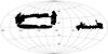 |
Fig. 1 The space distribution in equatorial coordinates of the SDSS-III DR9 data release quasars. |
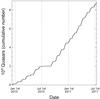 |
Fig. 2 Cumulative number of quasars as a function of observation date during the first two years of the survey. Horizontal times are due to the yearly summer shutdown during monsoon rains (summer 2010 at MJD = 55 400) and the monthly bright time when BOSS does not observe. |
As z > 2 quasars are usually identified by the presence of strong Lyman-α and C iv emission lines, we determine the S/N effectively achieved at the position of these lines. The median S/N per pixel at the position of various emission lines (Lyman-α, C iv, C iii] complex and Mg ii) and in the continuum are shown in Fig. 3. While the S/N per pixel in regions free of emission lines (black histogram) drops to be equal to ~1 at r ~ 22, the S/N at the top of the Lyman-α (green histogram) and C iv (red histogram) emission lines stays above about 4, allowing the identification of a fair fraction of these objects at this magnitude.
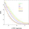 |
Fig. 3 Median observed S/N per pixel at the top of the Lyman-α (green), C iv (red), C iii] complex (blue), Mg ii at z > 2 (orange) and Mg ii at z < 2 (yellow) emission lines and in emission-line free regions (black) versus r-PSF magnitude (corrected for Galactic extinction). Two redshift ranges are considered for Mg ii because the emission line is redshifted in regions of the spectra with very different characteristics. At r ~ 22, the median S/N per pixel at the top of the Lyman-α and C iv emission lines is about 4; sufficient to identify most of the quasars. Outside of the emission-line regions, at the same magnitude, the S/N per pixel is about unity. |
In order to classify the object, each spectrum is fit by the BOSS pipeline2 with a library of star templates, a PCA decomposition of galaxy spectra and a PCA decomposition of quasar spectra. Each class of templates is fit over a range of redshifts: galaxies from z = −0.01 to 1.00 quasars from z = 0.0033 to 7.00; and stars from z = −0.004 to 0.004 (± 1200 km s-1). The combination of redshift and template with the overall best fit (in terms of the lowest reduced chi-squared) is adopted as the pipeline classification (CLASS) and redshift measurement (Z ± Z_ERR). A warning bitmask (ZWARNING) is set to indicate poor wavelength coverage, negative star template fits, broken/dropped fibers, fibers assigned to mesure sky background, and fits which are within Δχ2/d.o.f. = 0.01 of the next best fit (comparing only fits with a velocity difference of 1000 km s-1). A ZWARNING equals to zero indicates a robust classification with no pipeline-identified problem (Aihara et al. 2011; Bolton et al. 2012).
The classifications by the BOSS pipeline are not perfect however and visual inspection is required. Most misclassified spectra have low S/N. At S/N per pixel ~2, some objects are fit equally well by a star and a quasar template. Even if the object is correctly identified as a quasar, the redshift can be erroneous, because one line is misidentified; the most common case is Mg iiλ2800 is misidentified as Lyman-α. But this can be also because of a strong absorption feature (e.g. a damped Lyman-α system, DLA, or a BAL) spoils the profile of an emission line and the pipeline is unable to recover it.
2.4. Calibration warnings
2.4.1. Excess flux in the blue
The BOSS spectra often show excess light at the blue end (a similar problem was found in SDSS-DR7 spectra; Pâris et al. 2011).
To quantify this problem we selected spectra where a damped Lyman-α system (DLA) is observed with aborption redshift greater than 3.385 and with a column density N(H i) ≥ 1020.5 cm-2. There are 402 such quasars in the sample. In these spectra, and because of the presence of the DLA, the flux is expected to be zero at λobs ≤ 4100 Å (e.g. below the Lyman limit of all DLAs). When stacking the selected lines of sight (Fig. 4), we note instead that the flux increases for wavelengths below 4000 Å. The excess light at λobs ~ 3600 Å is 10% of the flux at λrest = 1280 Å where the spectra are normalized. This problem can affect the analysis of the Lyman-α forest (see e.g. Font-Ribera et al. 2012) and is probably a consequence of imperfect sky subtraction (Dawson et al. 2012). It will be corrected in a future version of the pipeline.
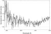 |
Fig. 4 Stack of DR9 BOSS spectra where a damped Lyman-α system is seen at an absorpstion redshift higher than 3.385 with a column density N(H i) ≥ 1020.5 cm-2. The spectra are normalized to unity near 1280 Å in the quasar rest frame. Owing to the presence of the DLA, the flux is expected to be zero at observed wavelengths below ~4100 Å (e.g. below the Lyman limit of all DLAs). This is not the case in the very blue part of the spectrum (λobs ≤ 4000 Å) where the mean observed flux appears to increase (spuriously). |
2.4.2. Spectrophotometric calibration
To maximize the flux in the blue part of the quasar spectra, where the Lyman-α forest lies, it was decided to offset the position of the quasar target fibers to compensate for atmospheric refraction and different focus in the blue (Dawson et al. 2012). These offsets were not applied to the standard stars. The current pipeline flux calibration does not take these fiber offsets into account, therefore the spectrophotometry of the main QSO targets (e.g. not the ancillary targets) is biased toward bluer colors over the full wavelength range. Spectrophotometry of these objects will preferentially exhibit excess flux relative to the SDSS imaging data at λ < 4000 Å and a flux decrement at longer wavelengths. Because the fiber offsets are intended to account for atmospheric differential refraction, data will show larger offsets in spectrophotometric fluxes relative to imaging photometry for observations performed at higher airmass. Dawson et al. (2012) discuss in details the quality of the BOSS spectrophotometry and reports that stellar contaminants in the quasar sample (i.e. quasar candidates that are actually stars) have g − r colors 0.038 mag bluer than the photometry with an rms dispersion of 0.158 mag.
This problem is illustrated in Fig. 5 where the median composite spectra of quasars observed by both SDSS-I/II and BOSS are plotted together. The resulting SDSS-DR7 spectrum is in red and BOSS spectrum in black. The BOSS composite spectrum is bluer than the same composite from SDSS-DR7 spectra. Note that this flux mis-calibration is different from object to object so that Fig. 5 shows only the mean difference between DR7 and DR9 spectra.
2.4.3. Identified quasars with bad spectra
During the course of the first two years of BOSS, different versions of the SDSS spectroscopic pipeline were used after some systematic problems had been fixed, thus improving the overall quality of the data. The visual inspection described below is performed on the fly, within a few days after the data are obtained, qualified and reduced by the version of the pipeline that is available at the time the data are obtained. Once an object is positively identified as a quasar, a galaxy, or a star from visual inspection, it keeps its identification in our catalog unless an apparent mistake has been committed and is corrected in the course of some check performed afterwards by the scanners or by a user of the data.
When a new version of the pipeline is made available, all the data are re-reduced. We then reinspect objects with uncertain identifications (QSO_?, QSO_Z?, Star_?, see Sect. 3.2) or spectra that are not qualified (Bad) but we do not reinspect the objects with firm identifications.
It can happen that the spectra of a few objects are of lesser quality with the new version of the pipeline. These objects are still in the catalog.
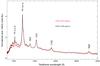 |
Fig. 5 Composite spectra of 6459 quasars observed both by SDSS-DR7 and BOSS for (i) SDSS-DR7 spectra (red) and; (ii) SDSS-DR9 spectra (black). The slope of the two composite spectra should be similar (as any variability should be averaged out). This is not the case because of the difference in focus of the BOSS quasars and standard stars. Note that this flux mis-calibration is different from object to object. |
Even the most thorough work of the kind described here cannot be absolutely flawless. We encourage the reader to signal any mistake to the first author of this paper in order to ensure highest quality of the information provided in the catalog.
3. Construction of the DR9Q catalog
In order to optimally measure the BAO clustering signal in the IGM, we must have as pure a catalog of quasars as possible. In this catalog, peculiar features such as broad absorption lines (BAL) or damped Lyman-α systems (DLA) that may dilute the signal, should be identified. We therefore designed quality control of the data based on a visual inspection of the spectra of all BOSS objects that might be a quasar. During commissioning and the first year of the survey this quality control was also very useful to report problems with the pipeline, which helped improve the overall quality of the data reductions.
The catalog lists all the visually confirmed quasars. About 10% of these quasars have been observed several times (Dawson et al. 2012), either because a particular plate has been re-observed (e.g. to increase the S/N for a particular scientific project), or because a particular region in the sky has been reobserved at different epochs (e.g. Stripe 82), or, because plates overlap. Now, and throughout BOSS, overlapping plates are used as an opportunity to increase the S/N on a few objets (e.g. CORE objects). These repeat observations are often useful to confirm the nature of objects with low S/N spectra. However we did not attempt to co-add these data mostly because they are often of quite different S/N.
3.1. A tool for the visual inspection
Immediately after the processing by the BOSS pipeline, the reduced data (spectra and pipeline classification) are copied to the IN2P3 (Institut National de Physique Nucléaire et de Physique des Particules) computing center3. A Java program gathers meta-information and saves it into an Oracle database.
All spectra are matched to target objects, imaging and photometry information, and SDSS-II spectroscopy. They are processed by a Java program that computes basic statistics from the spectra and fits a power law continuum and individual emission lines to each spectrum. The spectra are then made available online through a collaborative web application, from which human scanners can flag objects and decide classifications.
This tool and the visual inspection procedure described in the next section evolved with time during commissioning and the first six months of the survey. The whole procedure was repeated at the end of the first two years to guarantee the homogeneity of the catalog.
3.2. Visual inspection procedure
The identifications provided by the BOSS pipeline are already very good. Nevertheless about 12% of all quasar targets have a non-zero ZWARNING flag, i.e. their redshift is not considered to be reliable by the pipeline. After visual inspection, 4% of all confirmed quasars have a non-zero ZWARNING flag. Not surprisingly, the fraction of these objects increases with magnitude (see Fig. 6).
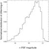 |
Fig. 6 Fraction of visually confirmed quasars with a non-zero ZWARNING flag as a function of the r-PSF magnitude (after correcting for Galactic extinction). A positive ZWARNING means that the pipeline considers its redshift estimate to be unreliable. This fraction increases at faint magnitudes. |
We visually inspected all quasar candidates and objects from quasar ancillary programs (see Sect. 2.2) to (i) secure the identification of the object and; (ii) reliably estimate the systemic redshift of the quasar. We manually confirmed or modified the identification of the object and, when needed, corrected the redshift provided by the BOSS pipeline, i.e. when it was wrong (when e.g. an emission line is misidentified or a bad feature was considered an emission line) or inaccurate (when emission lines are correctly identified but not properly centered). Examples of misidentified objects or inaccurate redshift estimates are displayed in Fig. 7.
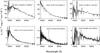 |
Fig. 7 First column: examples of z > 2 quasars classified as STAR by the BOSS pipeline. The overall shape of the spectrum is similar to the spectrum of F stars. Second column: examples of stars identified as QSO by the BOSS pipeline. Strong absorption lines or wiggles in the spectrum can mimic quasar features. Third colum: examples of z > 2 quasars for which the BOSS pipeline provides an inaccurate redshift estimate that must be corrected during the visual inspection. The pipeline is confused by the strong absorption lines. The spectra were boxcar median smoothed over 5 pixels. |
All the information on the objects is stored in a database which is updated in real time as new data arrives from the telescope. Modifications from the visual inspection are stored also in the database. For each plate, the objects classified by the pipeline as star, QSO with z < 2, and QSO with z ≥ 2 are made available to the scanner in three different lists. The cut in redshift corresponds to the Lyman-α emission line entering the BOSS spectrum. It also corresponds to a strong gap in the BOSS quasar redshift distribution due to target selection (see Fig. 22).
Most of the objects classified as stars by the pipeline are indeed stars and most of the objects classified as quasar with z < 2 are either quasars with z < 2 or stars (see below). The objects classified as quasars at z ≥ 2 are ranked by decreasing S/N. This organizes the visual inspection and minimizes the risk of errors. Most of the quasars with z ≥ 2, the most valuable for the survey, are inspected by two different individuals.
Objects that cannot be firmly identified by visual inspection are labeled in several categories. Some spectra cannot be recognized because either the S/N is too low, or the spectrum has been badly extracted; such objects are classified as Bad. For others, the classification is not considered to be robust, but there is some indication that they are stars (star_?) or quasars (QSO_?). For some objects both scanners were unable to give a firm identification, such objects are labeled as “?”. Other objects are galaxies (Galaxy). Finally some objects are recognized as quasars but their redshifts are not certain (QSO_Z?).
The output of the visual classification is provided as fields class_person and z_conf_person in the specObjAll table of the SDSS Catalog Archive Server (CAS) or the specObjAll.fits file from the Science Archive Server (SAS). The correspondence between the visual inspection classification we describe in this paper (QSO, QSO_BAL, QSO_Z?, QSO_?, Star, Star_?, Galaxy, ?) and the values of z_conf_person and class_person is given in Table 1. Each time a new version of the BOSS pipeline becomes available, the data are reprocessed and objects in the categories bad, ?, QSO_? and QSO_Z? are inspected again. Examples of objects classified as QSO_Z? and QSO_? are displayed in Fig. 8. Only objects classified as QSO or QSO_BAL are listed in the official DR9Q catalog. Objects classified as QSO_Z? are included in the supplemental list of quasars (see Sect. 8). Objects classified as QSO_? are also given for information in a separate list.
Of the 180 268 visually inspected targets corresponding to the DR9Q catalog, 87 822 were classified as unique quasars, 81 307 as stars and 6120 as galaxies. 1362 objects are likely quasars (QSO_?), 112 are quasars with an uncertain redshift (QSO_Z?) and 578 are likely stars (Star_?). 2599 targets have bad spectra (Bad) while we were not able to identify 368 objects (?). Therefore 97.5% of the objects are successfully classified. Only 27 true quasars were mis-identified by the BOSS pipeline as Star, while 11 523 stars were classified as QSO, most of them misidentified, however, as low redshift quasars, and only 1241 have ZWARNING = 0. Table 2 gives a summary of these numbers.
Note that Palanque-Delabrouille et al. (2012) have obtained deeper MMT QSO data of some of the BOSS targets classified as QSO_? and confirmed that essentially all of these objects are true quasars.
During the visual inspection, a redshift is determined that will be refined further by an automatic procedure (see Sect. 4). The redshift of identified quasars provided by the visual inspection is obtained applying the following procedure:
-
The first guess for the redshift is given by theBOSS pipeline and is not modified except ifinaccurate or wrong. The redshift from the pipeline can bewrong in cases where an emission line is misidentified. The pres-ence of strong absorption at ornear the emission, and especially astrong DLA, is alsoa source of error. Often the redshift is just inac-curate because either it misses the peak of theMg ii emissionline (and we consider that this lineis the most robust indicator of the redshift) or it isdefined by the maximum of theC iv emission line whenwe know that this line is often blueshifted compared toMg ii (Gaskell 1982; McIntoshet al. 1999; VandenBerk et al. 2001; Richardset al. 2002; Shenet al. 2008; Hewett& Wild 2010).
-
If the Mg ii emission line is present in the spectrum, clearly detected, and not affected by sky subtraction, the visual inspection redshift is set by eye at the maximum of this line. The typical uncertainty is estimated to be Δz < 0.003. The redshift is refined further, as described below.
Table 1Classification from the visual inspection corresponding to the combination of class_person (first column) and z_conf_person (first row) values provided in the headers of the SDSS-DR9 spectra available from the SDSS Catalog Archive Server.
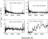
Fig. 8 Examples of QSO_? (top panels) and QSO_Z? (lower panels). The spectra were boxcar median smoothed over 5 pixels.
-
In other cases and for z > 2.3 quasars, such that Mg ii is redshifted into the noisy part of the red spectrum where sky subtraction errors make it unreliable, the redshift is estimated using the positions of the red wing of the C iv emission line which is known to be often blueshifted compared to Mg ii and of the peak of the Lyman emission line. The precision is estimated to be Δz < 0.005.
The visual redshift is not accurate to better than Δz ~ 0.003. but can be used as a reliable guess for further automatic redshift determination (see Sect. 4). Figure 9 displays the distribution of the velocity difference between the visual inspection redshift estimate and the redshift provided by the BOSS pipeline. At z ≤ 2 the pipeline estimate is usually good and does not require significant adjustments. In the redshift range 2.0−2.3, about half of the redshifts are modified because the Mg ii emission line is available and defines clearly the visual inspection redshift while the pipeline finds often a slightly lower redshift. At z ≳ 2.3, 10% of the redshifts are corrected. Only 1116 quasars (~2%), regardless of ZWARNING flags, have a difference between the pipeline and visual redshifts larger than 0.1.
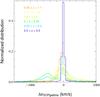 |
Fig. 9 Normalized (to unit integral) distribution of the velocity difference between the pipeline and visual inspection redshift estimates for different redshift bins. About half of the pipeline redshifts are corrected during the visual inspection. Most of the corrections are for quasars with 2 < z < 2.5 where the Mg ii emission line is available and where the pipeline redshift estimate does not correspond to the peak of the Mg ii emission line. |
In addition, peculiar spectral features are flagged:
-
When a damped Lyman-α absorption line is presentin the forest, the object is assigned a flag “DLA”. This flag can beused to check automatic Damped Lyman-α detections (see Noterdaeme et al. 2009, 2012).
-
Broad absorption lines in C iv and/or Mg ii are also flagged. At this point there is no estimate of the width of the lines and we stay conservative. This flag can be used to check automatic BAL detections (see Sect. 5.1).
-
Problems such as the presence of artificial breaks in the spectrum, obviously wrong flux calibration, or bad sky subtraction are flagged as well whatever the identification of the object is. These quality flags are pipeline-version dependent and are not meant to be released with the catalog. They are mainly useful for feedback to the pipeline team.
Number of objects identified as such by the pipeline with any ZWARNING value (second column) and with ZWARNING = 0 (third column), and after the visual inspection (fourth column).
3.3. A note on damped Lyman-α systems
In the course of the visual inspection, we flag the spectra with strong H i absorption (DLAs) in the Lyman-α forest. At this point we do not try to measure the column density or to determine the redshift of the DLA. Flagging these lines of sight can be useful to complement the search for DLAs by automatic procedures since this is a notoriously difficult task. Figure 10 shows the number of DLAs we flag along SDSS-DR7 lines of sight reobserved by BOSS, versus the N(H i) column density. It can be seen that we visually recover most of the DLAs (log N(H i) > 20.3) identified in the SDSS-DR7 by Noterdaeme et al. (2009). Only 11 such DLAs are missed by the visual inspection out of 257. The detection and analysis of DLAs in BOSS spectra is beyond the scope of this paper and will be described in Noterdaeme et al. (2012).
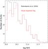 |
Fig. 10 H i column density distribution for DLAs and sub-DLAs detected by Noterdaeme et al. (2009) in quasars observed both by SDSS-DR7 and BOSS (black histogram). The red histogram displays the same distribution but for DLAs flagged after visual inspection of BOSS spectra. This shows that the visual inspection is robust for log N(H i) > 20.3, the standard definition of DLAs. |
4. Automatic redshift estimate
The visual inspection provides a reliable and secure redshift estimate for each quasar. Nevertheless, it is somewhat subjective and the accuracy of such an estimate is limited and cannot be better than 500 km s-1. In principle, it is possible to estimate the redshift of a quasar using a linear combination of principal components to fit the spectrum: the well known systematic shifts between emission lines are intrinsically imprinted in the components and the method can take into account the variations from quasar to quasar (see e.g. Pâris et al. 2011). This should be a reliable procedure providing:
-
the reference sample used to derive the principal components isrepresentative of the whole quasar population;
-
the redshift of each quasar in the reference sample is reliable.
We will derive PCA components in order to reproduce the quasar spectrum between 1410 and 2900 Å, in the quasar rest frame, so that most of the prominent emission lines are covered, especially C iv and Mg ii. This will yield an automatic estimate of the quasar redshifts. These components will be also used to fit emission lines individually to estimate a redshift for each emission line from the peak of the fit model. To derive these PCA components, we will use a reference sample of quasars for which the two main emission lines are well observed. The redshifts of the quasars in the reference sample have also to be chosen carefully. The technique to derive PCA components of quasar spectra has been described in detail in several papers (e.g. Francis et al. 1992; Yip et al. 2004; Suzuki et al. 2005). We refer the reader in particular to Sect. 2.3 of Pâris et al. (2011).
4.1. Selection of the reference sample
To compute a set of principal components from a sample as representative as possible of the whole quasar population, we selected quasar spectra in SDSS-DR7 meeting the following requirements:
-
The rest frame wavelength range 1410–2900 Å isredshifted into the observed wavelength range 3900–9100 Å (i.e. 1.77 < z < 2.13). This observed wavelength range is chosen to avoid the flux-excess issue in the very blue portion of the spectra (Sect. 2.4.1 and Pâris et al. 2011) and bad sky line subtraction at the red end.
-
The median squared S/N per pixel over the full wavelength range is higher than 5.
-
The spectra do not display BAL troughs as listed in the Allen et al. (2011) catalog.
In SDSS-DR7, 8986 quasar spectra meet these requirements. They all were visually inspected to remove spectra with obvious reduction issues (missing pixels, continuum breaks or very bad flux calibration). We finally used 8632 spectra.
The low-S/N cut we use here maximizes the number of quasars used for the PCA decomposition and makes our sample as representative as possible of the BOSS quasars.
4.2. Computing principal components
We now need an accurate redshift for each quasar before we calculate the PCA eigenvectors. We first describe the use of Hewett & Wild (2010) redshifts and then an improved approach using the peak of the Mg ii emission line in individual spectra.
Using Hewett & Wild (2010) redshifts:
We first consider the redshifts provided by Hewett & Wild (2010; HW10). They have performed a systematic investigation of the relationship between different redshift estimation schemes and have derived empirical relationships between redshifts based on different emission lines. They generated a high-S/N quasar template covering the UV and optical bands to be used to calculate cross-correlation redshifts. They estimate and correct for the quasar luminosity-dependence of systematic shifts between quasar emission lines. They are thus able to reduce systematic effects dramatically, correcting redshifts for the mean systematic shifts between emission lines. Note however that this does not fully account for intrinsic quasar-to-quasar variation among the population.
Using these redshifts for the sample of representative quasars defined in Sect. 4.1, we derive the PCA eigenvectors. We then use the set of principal components to fit a linear combination of 4 principal components to the whole spectrum of z ≥ 2.2 SDSS-DR7 quasar spectra and estimate their redshifts. This number of components has been chosen after several trials in order to be able to derive a robust redshift for the maximum of objects. Note that the samples used to compute the principal components and to which we apply the procedure are disjoint.
The median of the distribution of the velocity differences between the redshift given by HW10 and our redshift estimate is less than 30 km s-1. However, the rms of this distribution is about 1200 km s-1 which is undesirably large and is presumably due to quasar to quasar variations in emission-line shifts.
We can try to overcome this drawback by using a redshift that is more representative of the individual characteristics of the quasars in the reference sample. This is why we will derive a redshift from the observed Mg ii emission line in each quasar spectrum. Indeed this line has been recognized as a reliable indicator of the actual redshift of the quasar (Shen et al. 2007, HW10).
Using Mg ii emission line redshifts:
Using the set of PCA components previously described, we fit the Mg ii emission line of each quasar in the same SDSS-DR7 reference sample. From this fit, we define the Mg ii redshift using the peak-flux position of the emission line fit. Using a combination of principal components to fit an emission line avoids the need to assume a line profile (e.g. Gaussian, Lorentzian or Voigt).
To estimate the quality of each emission line fit:
-
We compute the amplitude of the emission line (expressed in unitsof the median error pixel of the spectrum in the window we use to fitthe line) from the maximum flux relative to a fitted power-lawcontinuum.
-
We measure the FWHM of the emission line in km s-1.
The amplitude-to-FWHM ratio (expressed in s km-1) provides an estimate of the prominence of the emission line. In particular, a weak and broad emission line will display a very low value of the amplitude-to-FWHM ratio.
To confirm the quality of the Mg ii line measurement, we also fit C iv emission lines using the same procedure. The C iv emission line is easier to fit since it is stronger and the region of the spectrum where it is redshifted is cleaner. If C iv could not be fit, we also considered the Mg ii fit to be unreliable.
We then used the 7193 spectra with both C iv and Mg ii amplitude-to-FWHM ratios larger than 8 × 10⁻⁴ s km-1 to compute the new PCA components to be applied to the whole spectra.
We use the set of principal components derived with the Mg ii redshifts in the following. Figure 11 displays the mean spectrum together with the first five principal components.
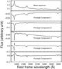 |
Fig. 11 Mean spectrum and the first five principal components derived in Sect. 4.2. A linear combination of the first four principal components is used to estimate the global redshift of the quasar, while five components are used to fit emission lines locally. |
4.3. Redshift estimates for BOSS quasars
For each quasar in the DR9Q catalog, we use four principal components to fit the overall spectrum after having subtracted the mean spectrum. Four components are enough to reproduce the overall shape of the spectrum and derive the redshift (Yip et al. 2004; Pâris et al. 2011). However, in order to avoid poor fitting due to the presence of strong absorption lines and especially BAL troughs, we first obtain a fit with only two principal components. This number is chosen because it provides a reasonable estimate of the amplitude of emission lines. Using this first guess, we remove pixels below 2σ and above 3σ of the continuum where σ is defined as the median flux error in an 11 pixel window. We are thus able to remove broad absorption lines and badly subtracted sky emission lines (especially at the very red end of the spectra). We then increase the number of principal components iteratively to three and four, removing narrow absorption lines, keeping the same detection thresholds.
Then, taking the visual inspection redshift estimate as an initial guess, it is possible to determine a redshift for each quasar by fitting a linear combination of four principal components to the spectrum, in which the redshift becomes a free parameter. We call this redshift the PCA redshift.
In addition, and in the same way as described in the previous subsection, we used five principal components to fit the Mg ii emission line in BOSS spectra when possible and derived a redshift from the peak flux of the fit model. Using PCA allows to recover the line without a priori assumptions about the line profile in a region of the spectrum affected by sky subtraction. In the following we will call this redshift the PCA Mg ii redshift estimate.
We compare in Fig. 12 the distributions of the velocity difference between PCA and PCA Mg ii redshift estimates. The PCA was applied to all BOSS quasars with 1.57 < zvisual < 2.3 so that both C iv and Mg ii emission lines are in the observed redshift range and are not strongly affected by sky subtraction. We considered three PCA estimates, varying the rest frame wavelength range over which the PCA was applied: (i) 1410−2850 Å (full range); (ii) 1410−2500 Å (Mg ii is not included) and (iii) 1410−1800 Å (only C iv is in the range). There are 18 271 objects. It can be seen in Fig. 12 that the distributions are very similar. The median and rms of the distributions are (−35.3, 642), (−52.2, 780) and (−30.3, 851) km s-1 respectively for the three wavelength ranges. The rms is dominated by low S/N spectra and slightly increases when the amount of information decreases. The similarity of the distributions clearly shows that the PCA redshift estimate is consistent with the Mg ii estimate even when Mg ii is not included in the fit.
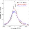 |
Fig. 12 Distributions of the velocity difference between PCA redshift estimates derived using different rest frame wavelength ranges and the PCA Mg ii redshift estimate. |
4.4. Comparison to HW10
In order to compare the HW10 redshift estimates to ours, we selected SDSS-DR7 quasars re-observed by BOSS in the redshift range 2.00 < z < 2.30. We also restricted the sub-sample to quasars for which we were able to fit the Mg ii emission line reliably and required the amplitude-to-FWHM of this line be larger than 8 × 10⁻⁴ s km-1. Even though the Mg ii emission line is still detectable up to z = 2.5, we restrict the redshift range to below z = 2.3 to avoid the red end of the spectra where sky lines can be badly subtracted. 746 quasar spectra remain for the comparison.
Figure 13 displays the distributions of velocity differences between the PCA Mg ii redshift estimate and our PCA global estimate (black histogram) or HW10 redshift (red histogram). Both distributions were normalized in the same manner and we also took into account the difference in the rest frame wavelength used by the different authors.
The median HW10 redshift estimate is shifted by +136.9 km s-1 (with positive velocity indicating redshift) compared to our median Mg ii redshift with an rms of 467 km s-1. Both HW10 and Shen et al. (2011) find that the median shift of the Mg ii emission line relative to the [OIII] doublet is smaller than 30 km s-1. These discrepancies in the median velocity shift may not be very significant as different fitting recipes for any of these lines (Mg ii, [OIII], C iv) can potentially cause systematic velocity differences of this order.
The median shift of our global estimate compared to the Mg ii redshift is −49.9 km s-1, with an rms of 389 km s-1. The rms of the distribution is smaller than previously because we restrict our comparison here to spectra with high S/N. It is more peaked and the number of outliers is lower. This is not surprising as we use the same components to fit the overall spectrum. However this illustrates the intrinsic dispersion between the results from the two methods.
The overall conclusion is that our PCA estimate is very close to the Mg ii emission line redshift. And we are confident that the application of the procedure using PCA components to quasars for which the Mg ii emission line is redshifted beyond the observed wavelength range, will give robust redshift estimates.
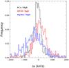 |
Fig. 13 Normalized distributions of the velocity difference between our global PCA redshift estimate (black histogram), the pipeline redshift estimate (blue histogram) or Hewett & Wild (2010) redshifts (red histogram) with the redshift derived from a PCA fit of the Mg ii emission line (see text). |
4.5. Emission line redshifts
Following the procedure described above, it is possible to reproduce the shape of each emission line with a linear combination of principal components. This combination can therefore fit the individual lines without any a priori assumption about the line profile. In the case of individual lines we have more flexibility to use more components because the fit is more stable over a smaller wavelength range. We will use five PCA components and define the position (redshift) of the line as the position of the maximum of this fit. Table 3 displays the definition of each window used to fit emission lines together with the vacuum rest frame wavelengths taken from the NIST database4 used to compute the redshift. For multiplets (e.g. C iv and Mg ii), the rest frame wavelength used is the average wavelength over the transitions in the multiplet weighted by the oscillator strengths. Together with the redshift estimate of each line, we also retrieve information on the symmetry of the line. We compute the blue (red) HWHM (half width at half maximum) from the PCA fit, bluewards (redwards) of its maximum. The total FWHM is the sum of the blue and the red HWHMs. The continuum is provided by the fit of a power law over the rest frame wavelength windows 1450−1500, 1700−1850 and 1950−2750 Å.
In Fig. 14 we plot the velocity of C iv relative to Mg ii versus the absolute magnitude of the quasar. The more luminous the quasar, the more blueshifted is the C iv emission line. Errors in the fit are less than 200 km-1. These measurements can be useful to understand the relative shifts between different emission lines and discuss the structure of the broad line region (see Shen et al. 2007; Shang et al. 2007).
The C iii]λ1909 line is blended with Si iii]λ1892 and to a lesser extent with Al iiiλ1857. We do not attempt to deblend these lines. This means that the redshift and red HWHM derived for this blend should correspond to C iii]λ1909, but the blue HWHM is obviously affected by the blend.
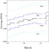 |
Fig. 14 Velocity difference between C iv and Mg ii emission line redshifts as a function of the absolute i magnitude of the quasar. The solid black line shows the median velocity shift in 0.2 mag bins. Blue and cyan histograms display the 10th, 30th, 70th and 90th percentiles. The mean shift between the two emission lines increases with the quasar luminosity. |
Window and rest frame wavelength used to fit each emission line.
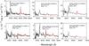 |
Fig. 15 Examples of high-redshift BAL quasar spectra in different ranges of S/N and BI. The fit of the continuum is overplotted. |
5. Broad absorption line quasars
Broad absorption troughs are flagged as BAL during the visual inspection. This flag means that an absorption feature broader than a usual intervening absorption (those arising in galaxies lying along the line of sight to the quasar) is seen. These BALs may affect the Lyman-α forest and should be removed from its analysis. We flag mostly C iv BALs but also Mg ii BALs. Since during the visual inspection we do not measure the width of the trough, there is no a priori limit on the strength of the absorption.
We also implemented an automatic detection of C iv BALs. We describe in Sect. 5.1 the method used to detect BALs and estimate their properties automatically. We then test the robustness of the visual inspection in Sect. 5.2 and the results of the automatic detection in Sect. 5.3.
In the following subsections, we will concentrate on C iv BALs with z > 1.57. The quasar redshift limit is chosen so that the Si iv emission line is included in the spectra. This ensures that C iv BALs can be measured across the full range of velocities in balnicity index, e.g. up to 25 000 km s-1.
5.1. Method used to estimate BAL properties automatically
In order to detect BALs and to characterize the strength of the troughs using an objective procedure, we compute the balnicity (BI, Weymann et al. 1991) and the absorption indices (AI, Hall et al. 2002) of the C iv troughs. In addition, we introduce a new index, the detection index (DI), which is a slight modification of BI. In Sect. 5.3, we will measure these indices for all quasars regardless of visual inspection.
The continuum has to be estimated first. For this, we use the same linear combination of four principal components described in Sect. 4. The resulting continuum covers the region from the Si iv to the Mg ii emission lines (see examples in Fig. 15). As described in Sect. 4.5, the procedure iteratively avoids absorption features and especially the BALs. During the automatic procedure, we smoothed the data with a five pixel boxcar median.
With this continuum, we compute the BI in the blue of the C iv emission line using the definition introduced by Weymann et al. (1991): ![Mathematical equation: \begin{equation} % {\rm BI} = - \int_{25\,000}^{3000}\left[ 1 - \frac{f(v)}{0.9} \right] C(v) \, {\rm d}v, \label{eq:BI} \end{equation}](/articles/aa/full_html/2012/12/aa20142-12/aa20142-12-eq103.png) (1)where f(v) is the flux normalized to the continuum as a function of velocity displacement from the line center. C(v) is initially set to 0 and can take only two discrete values, 0 or 1. It is set to 1 whenever the quantity 1 − f(v)/0.9 is continuously positive over an interval of at least 2000 km s-1. It is reset to zero whenever the quantity in brackets becomes negative. Therefore BI = 0 does not mean that no trough is present. It means that, if a trough is present, the absorption does not reach 0.9 times the estimated continuum over a continuous window of 2000 km s-1.
(1)where f(v) is the flux normalized to the continuum as a function of velocity displacement from the line center. C(v) is initially set to 0 and can take only two discrete values, 0 or 1. It is set to 1 whenever the quantity 1 − f(v)/0.9 is continuously positive over an interval of at least 2000 km s-1. It is reset to zero whenever the quantity in brackets becomes negative. Therefore BI = 0 does not mean that no trough is present. It means that, if a trough is present, the absorption does not reach 0.9 times the estimated continuum over a continuous window of 2000 km s-1.
We will also define DI giving C a value 1 over the whole trough if the criterion of a continuous trough over 2000 km s-1 is fulfilled. This index has the advantage of measuring the strength over the whole trough. This index will be useful to apply cuts in the analyses of the Lyman-α forest. Indeed these analyses need an estimate of the total strength of the trough in order to avoid lines of sight spoiled by a strong BAL.
To study weaker troughs, Hall et al. (2002) introduced the AI measurement defined as ![Mathematical equation: \begin{equation} % {\rm AI} = - \int_{25\,000}^{0}\left[ 1 - \frac{f(v)}{0.9} \right] C(v) \, {\rm d}v, \label{eq:AI} \end{equation}](/articles/aa/full_html/2012/12/aa20142-12/aa20142-12-eq107.png) (2)where f(v) is the normalized flux and C(v) has the same definition as for the DI except that the threshold to set C to 1 is reduced to 450 km s-1. The AI index was introduced in order to take into account weaker troughs and to measure troughs that are located close to the quasar rest velocity. It is however more sensitive to the continuum placement than the BI. Note that Trump et al. (2006) used a modified version of the AI wherein the factor of 0.9 was removed from the integral to make the AI an equivalent width measured in km s-1, where 1000 km s-1 was the threshold instead of 450 km s-1, and where the integral extended to 29 000 km s-1. In this work we use the original Hall et al. (2002) definition of the AI.
(2)where f(v) is the normalized flux and C(v) has the same definition as for the DI except that the threshold to set C to 1 is reduced to 450 km s-1. The AI index was introduced in order to take into account weaker troughs and to measure troughs that are located close to the quasar rest velocity. It is however more sensitive to the continuum placement than the BI. Note that Trump et al. (2006) used a modified version of the AI wherein the factor of 0.9 was removed from the integral to make the AI an equivalent width measured in km s-1, where 1000 km s-1 was the threshold instead of 450 km s-1, and where the integral extended to 29 000 km s-1. In this work we use the original Hall et al. (2002) definition of the AI.
Following Trump et al. (2006), we calculate the reduced χ2 for each trough: 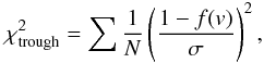 (3)where N is the number of pixels in the trough, f(v) is the normalized flux and σ the rms of the pixel noise. The greater the value of
  , the more likely the trough is not due to noise.
We apply the automatic detection to all quasars in the DR9Q catalog and provide values of DI, AI and BI. We estimate also an error on the indexes. The error squared is obtained by applying the same formula as for the indexes replacing (1 − f/0.9) by (σ/0.9)2 with σ the rms of the noise in each pixel. Note however that the error on the strength of the trough is most of the time dominated by the placement of the continuum. To estimate the latter we have displaced the fitted continuum by 5% and applied Eq. (2) of Kaspi et al. (2002).
5.2. Robustness of the visual detection of BALs
During the visual inspection, we are conservative and flag a BAL only if the trough is apparent. In addition, the automatic detections rely on the position of the continuum while the visual inspection lacks this problem. This means that the BAL sample from the visual inspection is purer than those from automatic detection. It is however unavoidable that, as the strength of the absorption or the spectrum S/N decreases, the visual inspection will start to be subjective. On the other hand the fraction of false BALs detected by the automatic procedure will be higher. Figure 16 shows the ratio of the number of visual BALs to that of the automatic detections as a function of S/N per pixel at λrest = 1700 Å for BI > 500 km s-1.
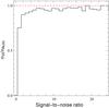 |
Fig. 16 Ratio of the numbers of BAL visual and automatic detections as a function of spectral S/N per pixel at λrest = 1700 Å for BI > 500 km s-1. As expected, this ratio decreases with decreasing S/N. |
Out of the whole DR9Q catalog, 7533 quasars have been flagged visually as BAL. Out of the 69 674 quasars with z > 1.57, 7228 are flagged as BAL by visual inspection. If we restrict the latter sample to quasars with S/N > 10 at 1700 Å in the rest frame we have flagged 1408 BALs out of 7317 quasars, a fraction of 19.2% which compares well with what was found by Gibson et al. (2009).
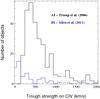 |
Fig. 17 Distribution of BI and AI for quasars detected as BAL by automatic procedures in previous SDSS releases, and that were not flagged by the visual inspection of the BOSS spectra. The black histogram shows the distribution of AI as measured by Trump et al. (2006) for 296 such quasars (all have BI = 0). About half of them are not real BALs (see text). From the automatic detection by Allen et al. (2011) (blue histogram), 57 quasars were missed by the visual inspection. Here again, only a handful of these objects actually display BAL troughs. |
Trump et al. (2006) measured BAL troughs (BI and AI) in the SDSS-DR3 release. We compare their detections and BI measurements with ours for quasars in common between BOSS and SDSS-DR3. Out of the 477 BALs (BI > 0) that are detected by Trump et al. (2006), we flag 425. We checked the BOSS spectra of these quasars individually. About half of them are not BALs and a handful, all with BI < 500 km s-1, are real BALs that were missed by the visual inspection. For the rest, it is hard to decide if they are real or not because of poor S/N. Note that, in general, BOSS spectra are of higher S/N than previous SDSS spectra.
There are an additional 296 quasars in Trump et al. (2006) that have C iv troughs that we do not flag as BALs. These all have AI > 0 but BI = 0. The histogram of AI measurements from Trump et al. (2006) for these objects is plotted as well in Fig. 17 (black histogram). Most of the missing troughs have AI smaller than 1000 km s-1. A visual inspection of the BOSS spectra reveals that most of the AIs have been overestimated and about half are not real mainly because the continuum in the red side of the C iv emission line has been overestimated.
Allen et al. (2011) searched for BALs in SDSS-DR6; they measured only BI. Out of the 7223 quasars with z > 1.57 in common with BOSS, they find 722 quasars with BI > 0. Of these 7223 objects, we flag 1259 as BALs of which 853 have BI > 0. We checked the 131 objects for which we measured BI > 0 but Allen et al. (2011) found BI = 0 individually. Some of the additional BALs are identified because of better S/N in BOSS, some were missed by Allen et al. (2011) because of difficulties in fitting the emission line correctly, a handful are explained by the disappearance of the BAL between the two epochs (Filiz Ak et al. 2012) and also by some appearances (see Fig. 18). We also find 57 objects that are detected by Allen et al. (2011) and are missing in our visual detection. The BI distribution of these objects is shown as the blue histogram in Fig. 17. About half of them are not BALs upon re-inspection and a handful are real BALs missed by the visual inspection. The nature of the rest of the objects is unclear.
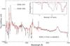 |
Fig. 18 Example of appearing BAL troughs. This quasar has been observed in SDSS-DR7 (red curve) and in SDSS-DR9 (black curve). The two spectra have been scaled to have a surface unity between 5600 and 6200 Å. The normalized flux in the C iv region expressed in velocity is displayed in the inset. This quasar had was not detected as BAL in SDSS-DR7 (i.e. BI = 0) while it has BI = 1826 km s-1 in the SDSS-DR9 spectrum. |
We conclude from this comparison that our catalog of BAL quasars flagged by visual inspection is pure at the 95% level, but is probably incomplete below BI ~ 500 km s-1. This results from the conservative approach we adopted when flagging the troughs implying that the number of detections in the visual inspection is decreasing with decreasing S/N.
It is difficult to estimate the incompleteness especially at low S/N because none of the previously published samples is reliable at small BI values. Therefore we caution the reader against blind uses of the catalog. S/N at rest wavelength 1700 Å (S/N_1700) is provided in the catalog. This can be used to identify the more reliable spectra.
The BI distributions normalized by the total number of quasars with BI > 500 km s-1 in each sample for visually flagged BALs in DR9 (this work) and DR6 (Allen et al. 2011) are compared in Fig. 19. We find 3130 BALs with BI > 500 km s-1 out of 69 674 BOSS quasars with z > 1.57 (4.5%). If we restrict ourselves to quasars with S/N > 10, these numbers are 813 BALs out of 7317 quasars, corresponding to a rate of 11.1%. This compares well with the ~10% uncorrected observed fraction of BAL found by Allen et al. (2011) at z ~ 2.5.
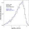 |
Fig. 19 Normalized distributions of the logarithm of BI measured from C iv troughs. The BI distribution from the present catalog (black histogram) computed from 7227 visually flagged BAL quasars is very similar to the distribution from Trump et al. (2006, red histogram) obtained from 1102 BAL quasars from the SDSS-DR3 quasar catalog (Schneider et al. 2005). The distribution is also very similar to the BI distribution from Allen et al. (2011, blue histogram) based on the SDSS-DR6 quasar catalog. |
5.3. Automatic detection
We also performed an automatic detection of the C iv troughs using the continua in the wavelength range between the Si iv to C iv emission lines computed as described in Sect. 4. BIs, AIs and DIs are calculated for all quasars with z > 1.57 using Eqs. (1) and (2). The values are given in the catalog together with the number of troughs both with width > 2000 and 450 km s-1. We also give, for quasars with BI > 0, the minimum and maximum velocities relative to zem, vmin and vmax, spanned by the whole absorption flow.
Out of the 69 674 (resp. 7317) quasars with z > 1.57 (resp. and S/N_1700 > 10), 8124 (resp. 3499) BALs, with > 10, have AI > 0 km s-1. A visual inspection of spectra with small values of AI indicates that a number are due to inadequate continuum fitting. We advise to be careful with AI values smaller than 300 km s-1 (see also below).
Out of the 69 674 (resp. 7317) quasars with z > 1.57 (resp. and S/N_1700 > 10), 4855 (resp. 1196) BALs have BI > 0 km s-1. This corresponds to 7% (resp. 16.3%). 821 BALs (11.2%) have BI > 500 km s-1. While the overall detection rate is larger than for the visual inspection, it is important to note that the automatic detection finds only 8 more objects with BI > 500 km s-1 in spectra with S/N > 10 than the visual inspection. Upon reinspection, we found that half of them are not real and are due either to a peculiar continuum or to the presence of strong metal lines from a DLA at zabs ~ zem. Three are real, but shallow BALs. This shows that the automatic and visual detections give nearly identical results for BI > 500 km s-1. At lower BI and lower S/N, and consistently with what was found by comparison with previous surveys, the number of unreliable detections is large.
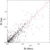 |
Fig. 20 Balnicity index (BI) from this work against BI measured by Allen et al. (2011) for SDSS-DR6 objects re-observed by BOSS. |
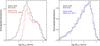 |
Fig. 21 Left panel: distribution of AI from our automatic detection (black histogram) and from SDSS-DR3 (red histogram, Trump et al. 2006). The distributions are normalized for log AI > 3. The difference between the two results at low AI is a consequence of slightly different formula used to measure AI. Right panel: distribution of BI from our automatic detection (black histogram) and from SDSS-DR6 (blue histogram, Allen et al. 2011). |
We compare in Fig. 20 the BI values measured by Allen et al. (2011) for SDSS-DR6 spectra with BI values measured by our automatic procedure using BOSS spectra for the same quasars. Although the scatter is large, the median difference is only ~30 km s-1. Note that part of the scatter is probably due to BAL variability (see Gibson et al. 2008, 2010; Filiz Ak et al. 2012). In Fig. 21 left (resp. right) panel, we compare the frequency distribution of AI (resp. BI) values in our BAL sample detected automatically with that of previous studies. The distributions are normalized in the same manner. It can be seen that the shape of the distributions are very similar. They peak around AI = 300 km s-1 which is the lower limit we set for robust detection.
We have shown here that BI measurements provided in the catalog are robust for S/N > 5 (see Fig. 16) and BI > 500 km s-1. Any statistical analysis should be restricted to the corresponding sample. The catalog gives a few properties of detected C iv troughs and of Si iv and Al iii troughs but only in cases where BI(C iv) > 500 km s-1 and S/N > 5. These troughs have been measured by Gibson et al. (2009) in SDSS-DR5.
6. Description of the DR9Q catalog
The DR9Q catalog is available both as a standard ASCII file and a binary FITS table file at the SDSS public website http://www.sdss3.org/dr9/algorithms/qso_catalog.php. The files contain the same number of columns, the FITS headers contain all of the required documentation (format, name, unit of each column). The following description applies to the standard ASCII file. Table 4 provides a summary of the information contained in each of the columns in the ASCII catalog. The supplemental list of quasars (see Sect. 8) together with the list of objects classified as QSO_? are also available at the same SDSS public website.
Notes on the catalog columns:
-
1. The DR9 object designation, given by the formatSDSS Jhhmmss.ss+ddmmss.s; only the final 18characters are listed in the catalog (i.e., the“SDSS J”for each entry is dropped). The coordinates in the objectname follow IAU convention and are truncated,not rounded.
-
2–3. The J2000 coordinates (Right Ascension and Declination) in decimal degrees. The astrometry is from DR9 (see Ahn et al. 2012).
-
4. The 64-bit integer that uniquely describes the spectroscopic observation that is listed in the catalog (Thing_ID).
-
5–7. Information about the spectroscopic observation (Spectroscopic plate number, Modified Julian Date, and spectroscopic fiber number) used to determine the characteristics of the spectrum. These three numbers are unique for each spectrum, and can be used to retrieve the digital spectra from the public SDSS database.
-
8. Redshift from the visual inspection (see Sect. 3.2).
-
9. Redshift from the BOSS pipeline (see Sect. 2 and Bolton et al. 2012).
-
10. Error on the BOSS pipeline redshift estimate.
-
11. ZWARNING flag from the pipeline. ZWARNING > 0 indicates bad fits in the redshift-fitting code.
-
12. Automatic redshift estimate from the fit of the quasar continuum over the rest frame wavelength range 1410−2000 Å with a linear combination of four principal components (see Sect. 4). When the velocity difference between automatic PCA and visual inspection redshift estimates is larger than 3000 km s-1, this PCA redshift is set to −1. The inaccuracy in the PCA estimate is often due to difficulties in the fit of the continuum. In that case no automatic measurements are made on these objects and BI is set to −1.
Table 4DR9Q catalog format.
-
13. Error on the automatic PCA redshift estimate. If the PCA redshift is set to −1, the associated error is also set to −1.
-
14. Estimator of the PCA continuum quality (between 0 and 1). See Eq. (11) of Pâris et al. (2011).
-
15–17. Redshifts measured from C iv, C iii] complex and Mg ii emission lines from a linear combination of five principal components (see Sect. 4).
-
18. Morphological information. If the SDSS photometric pipeline classified the image of the quasar as a point source, the catalog entry is 0; if the quasar is extended, the catalog entry is 1.
-
19–21. Quasars targeted by BOSS are tracked with the BOSS_TARGET1 flag bits (19; see details of selection method in Ross et al. 2012). In addition, 5% of fibers on each plate are dedicated to ancillary programs tracked with the ANCILLARY_TARGET1 (20) and ANCILLARY_TARGET2 (21) flag bits. The bit values and the corresponding program names are listed in Dawson et al. (2012).
-
22. A quasar known from SDSS-DR7 has an entry equal to 1, and 0 otherwise
-
23–25. Spectroscopic plate number, Modified Julian Date, and spectroscopic fiber number in SDSS-DR7.
-
26. Uniform flag. See Sect. 7.4.
-
27. The absolute magnitude in the i band at z = 2 calculated after correction for Galactic extinction and assuming H0 = 70 km s-1 Mpc-1, ΩM = 0.3, ΩΛ = 0.7, and a power-law (frequency) continuum index of −0.5. The K-correction is computed using Table 4 from Richards et al. (2006).
-
28. The Δ(g − i) color, which is the difference in the Galactic extinction corrected (g − i) for the quasar and that of the mean of the quasars at that redshift. If Δ(g − i) is not defined for the quasar, which occurs for objects at either z < 0.12or z > 5.12the column will contain “−9.000”. See Sect. 7 for a description of this quantity.
-
29. Spectral index αν (see Sect. 7.2).
-
30. Median S/N computed over the whole spectrum.
-
31. Median S/N computed over the window 1650−1750 Å in the quasar rest frame.
-
32. Median S/N computed over the window 2950−3050 Å in the quasar rest frame.
-
33. Median S/N computed over the window 5100−5250 Å in the quasar rest frame.
-
34–37. FWHM (km s-1), blue and red HWHM (the sum of the latter two equals FWHM), and amplitude (in units of the median rms pixel noise, see Sect. 4) of the C iv emission line.
-
38–39. Rest frame equivalent width and corresponding uncertainty in Å of the C iv emission line.
-
40–43. Same as 34-37 for the C iii] emission complex. It is well known that C iii]λ1909 is blended with Si iii]λ1892 and to a lesser extend with Al iiiλ1857. We do not attempt to deblend these lines. Therefore the redshift and red HFHM derived for this blend correspond to C iii]λ1909. The blue HFWM is obviously affected by the blend.
-
44–45. Rest frame equivalent width and corresponding uncertainty in Å of the C iii] emission complex.
-
46–49. Same as 34–37 for the Mg ii emission line.
-
50–51. Rest frame equivalent width and corresponding uncertainty in Å of the Mg ii emission line.
-
52. BAL flag from the visual inspection. It is set to 1 if a BAL feature was seen during the visual inspection. It is set to 0 otherwise. Note that BAL quasars are flagged during the visual inspection at any redshift.
-
53–54. Balnicity index for C iv troughs, and its error, expressed in km s-1. See definition in Sect. 5.1. The BI is measured for quasars with z > 1.57 only. If the BAL flag from the visual inspection is set to 1 and the BI is equal to 0, this means either that there is no C iv trough (but a trough is seen in another transition) or that the trough seen during the visual inspection does not meet the formal requirement of the BAL definition. In cases with bad fits to the continuum, the BI and its error are set to −1.
-
55–56. Absorption index, and its error, for C iv troughs expressed in km s-1. See definition in Sect. 5.1. In cases with bad continuum fit, the AI and its error are set to −1.
-
57–58. Detection index, and its error, for C iv troughs expressed in km s-1. See definition in Sect. 5.1. In cases with bad continuum fit, the DI and its error are set to −1.
-
59. Following Trump et al. (2006), we calculate the reduced χ2 for each trough from Eq. (3). We require that troughs have
> 10 to be considered as true troughs (see Sect. 5.1). -
60. Number of troughs of width larger than 2000 km s-1.
-
61–62. Full velocity range over which C iv troughs are at least 10% below the continuum for troughs of width larger than 2000 km s-1.
-
63. Number of troughs of width larger than 450 km s-1.
-
64–65. Full velocity range over which C iv troughs are at least 10% below the continuum for troughs of width larger than 450 km s-1.
-
66–68. Rest frame equivalent width in Å of Si iv, C iv and Al iii troughs detected in BAL quasars with BI > 500 km s-1 and S/N_1700 > 5. They are set to 0 otherwise or in cases where no trough is detected and to −1 if the continuum is not reliable.
-
69–70. The SDSS Imaging Run number and the Modified Julian Date (MJD) of the photometric observation used in the catalog. The MJD is given as an integer; all observations on a given night have the same integer MJD (and, because of the observatory’s location, the same UT date). For example, imaging run 94 has an MJD of 51 075; this observation was taken on 1998 September 19 (UT).
-
71–74. Additional SDSS processing information: the photometric processing rerun number; the camera Cols. (1−6) containing the image of the object, the field number of the run containing the object, and the object identification number (see Stoughton et al. 2002, for descriptions of these parameters).
-
75–84. DR9 flux and errors (not corrected for Galactic extinction) in the five SDSS filters.
-
85–89. TARGET photometric flux in the five SDSS filters.
-
90. Galactic extinction in the u band based on the maps of Schlegel et al. (1998). For an RV = 3.1 absorbing medium, the extinctions in the SDSS bands can be expressed as
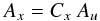 where x is the filter (ugriz), and values of Cg,r,i,z are 0.736, 0.534, 0.405, and 0.287. See Schlafly & Finkbeiner (2011) however.
 -
91. The logarithm of the Galactic neutral hydrogen column density along the line of sight to the quasar. These values were estimated via interpolation of the 21-cm data from Stark et al. (1992), using the COLDEN software provided by the Chandra X-ray Center. Errors associated with the interpolation are typically expected to be less than ≈ 1 × 1020 cm-2 (e.g., see Sect. 5 of Elvis et al. 1994).
-
92. The logarithm of the vignetting-corrected count rate (photons s-1) in the broad energy band (0.1−2.4 keV)in the ROSAT All-Sky Survey Faint Source Catalog (Voges et al. 2000) and the ROSAT All-Sky Survey Bright Source Catalog (Voges et al. 1999). The matching radius was set to 30′′ (see Sect. 7.5.1);
-
93. The S/N of the ROSAT measurement.
-
94. Angular Separation between the SDSS and ROSAT All-Sky Survey locations (in arcseconds).
-
95–98. UV fluxes and errors from GALEX, aperture-photometered from the original GALEX images in the two bands FUV and NUV (see Sect. 7.5.2).
-
99–100. The J magnitude and error from the Two Micron All Sky Survey All-Sky Data Release Point Source Catalog (Cutri et al. 2003) using a matching radius of 2.0′′ (see Sect. 7.5.3). A non-detection by 2MASS is indicated by a “0.000” in these columns. Note that the 2MASS measurements are Vega-based, not AB, magnitudes.
-
101–102. S/N in the J band and corresponding 2MASS jr_d flag.
-
103–106. Same as 98–101 for the H-band.
-
107–110. Same as 98–101 for the K-band.
-
111. Angular separation between the SDSS and 2MASS positions (in arcseconds).
-
112–113. The w1 magnitude and error from the Wide-field Infrared Survey Explorer (WISE; Wright et al. 2010) All-Sky Data Release Point Source Catalog using a matching radius of 2′′ (see Sect. 7.5.4).
-
114–115. S/N and χ2 in the WISE w1 band.
-
116–119. Same as 111–114 for the w2-band.
-
120–123. Same as 111–114 for the w3-band.
-
124–127. Same as 111–114 for the w4-band.
-
128. Angular separation between SDSS and WISE positions (in arcseconds).
-
129. If there is a source in the FIRST catalog (version July 2008) within 2.0′′ of the quasar position, this column contains the FIRST peak flux density (see Sect. 7.5.5). An entry of “0.000” indicates no match to a FIRST source; an entry of “−1.000” indicates that the object does not lie in the region covered by the final catalog of the FIRST survey.
-
130. The S/N of the FIRST source whose flux is given in Col. 128.
-
131. Angular separation between the SDSS and FIRST positions (in arcseconds).
7. Summary of sample
7.1. Broad view
The DR9Q catalog contains 87 822 unique, visually confirmed quasars, of which 65 205 and 61 931 have, respectively, z ≥ 2 and z > 2.15. 91% of these quasars were discovered by BOSS. The first two years of operations cover an area of approximately 3275 deg2 leading to a mean density of > 15 quasars with z > 2.15 per square degree. In the following, we describe the properties of the quasar population drawn from the whole sample. However, we also provide a uniform flag (see Sect. 7.4). A sample of quasars with uniform > 0 is a sufficiently statistical sample for, e.g., clustering measurements on some scales (e.g., White et al. 2012) and luminosity function demographics.
Quasars from the present catalog span a range of redshift from z = 0.058 to z = 5.855. The redshift distribution is given in Fig. 22 together with that from SDSS-DR7 (red histogram, Schneider et al. 2010). It is apparent from the figure that BOSS primarily targets z > 2.15 quasars as it was designed. Only 7932 of those quasars were previously known, e.g. detected by previous surveys and the majority of those were previous SDSS discoveries. The DR9Q catalog thus contains about 2.6 times more high-redshift quasars than the whole SDSS-I/II survey. The two peaks in the redshift distribution at z ~ 0.8 and z ~ 1.6 are due to known degeneracies in the SDSS color space. Six objects have z < 0.1. These are Seyfert galaxies that were classified as quasars in order to differentiate them from normal galaxies.
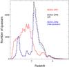 |
Fig. 22 The redshift distribution of quasars from this catalog is displayed in black. The same distribution is shown for newly discovered quasars only (dashed blue histogram). Most of the SDSS-DR9 quasars have a redshift greater than 2. The redshift distribution of quasars from the SDSS-DR7 catalog (Schneider et al. 2010) is shown for comparison in red. The latter is dominated by quasars at low redshift. The present catalog contains 2.6 times more quasars at z > 2.15 than the DR7 catalog. |
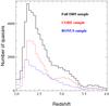 |
Fig. 23 Redshift distribution of SDSS-DR9 quasars in the range 2.00−4.00 for the whole distribution (black histogram), the CORE sample (red histogram) and the BONUS sample (blue histogram). The CORE sample was uniformly selected through the likelihood method (Kirkpatrick et al. 2011) during most of the first year of operation and the XDQSO method (Bovy et al. 2011) for the second year. The BONUS sample was selected through a combination of four target selection algorithms to maximize the number of high-redshift quasars in the sample. |
Figure 23 displays the redshift distributions in the redshift range of interest for BOSS for the whole sample (black histogram), the CORE sample (red histogram) and the BONUS sample (blue histogram). The CORE sample is selected via uniform target selection (see details in Ross et al. 2012), and is designed for statistical studies of the quasar population (see Sect. 7.4). On the other hand, the BONUS sample is the result of the combination of four target selection algorithms. This sample was designed to maximize the number of high-redshift quasars. Typical spectra are shown in Fig. 24.
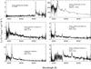 |
Fig. 24 First row, left: spectrum of the highest redshift quasar (z = 5.855) observed by BOSS; this quasar was discovered by Fan et al. (2004); the quasar with highest redshift discovered by BOSS is SDSS J222018.50−010147.0 at z = 5.605. First row, right: spectrum of the most luminous (Mi[z = 2] = −30.91) quasar available in this catalog. Middle and bottom rows: four typical quasar spectra selected to be representative in terms of S/N at different redshifts (z ~ 2.3, 2.5, 2.7, 3.5). The S/N listed is the median S/N per pixel over the whole spectrum. All the spectra were boxcar median smoothed over 5 pixels. |
Table 5 gives the number of objects targeted by the various selection methods and visually inspected (Col. #2) as described in Ross et al. (2012) together with the number of objects classified by visual inspection as quasars (Col. #3), quasars with z > 2.15 (Col. #5), stars (Col. #6) or galaxies (Col. #7). Columns #8 and #9 give, respectively, the number of objects with good spectra but uncertain identification and the number of objects with data of too low S/N to allow for identification (see Sect. 3 for a detailed description of the different categories). Note that a single object can be selected by several methods.
Number of visually inspected DR9 BOSS quasar targets (third column) and identifications in the DR9Q catalog for each target selection method (first column; see Table 4 of Ross et al. 2012, and Tables 6 and 7 in the Appendix of Dawson et al. 2012).
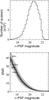 |
Fig. 25 Top panel: distribution of r magnitude of SDSS-DR9 quasars (PSF; corrected for Galactic extinction). Bottom panel: median S/N per pixel over the whole spectrum with respect to the r-PSF magnitude (black histogram). Percentiles are indicated in grey. |
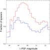 |
Fig. 26 Fraction of quasar candidates confirmed as quasars (red histogram) and z > 2.15 quasars (blue histogram) versus the i-band PSF magnitude (corrected for Galactic extinction). |
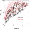 |
Fig. 27 L − z plane for SDSS-DR9 quasars (black contours and points) and SDSS-DR7 quasars (red contours and points; Schneider et al. 2010). The luminosity assumes H0 = 70 km s-1 Mpc-1 and the K-correction is given by Richards et al. (2006) who consider K(z = 2) = 0. Contours are drawn at constant point density. |
BOSS targets fainter objects than SDSS-I/II. The r-PSF magnitude distribution (corrected for Galactic extinction) of SDSS-DR9 quasars is shown in Fig. 25 (top panel), and peaks at ~20.8. The median S/N computed over the whole spectrum versus the r-PSF magnitude is shown in the bottom panel of Fig. 25. Percentiles are indicated in grey. The i-PSF magnitude distribution of quasar candidates, spectroscopically confirmed quasars and z > 2.15 confirmed quasars are shown in Fig. 26. There is no drop of the success rate at high magnitude, indicating again that the S/N threshold used to define a survey quality plate is well chosen.
Figure 27 shows the distribution of objects in the redshift-luminosity (L versus z) plane for the BOSS survey (black contours and points) together with the same quantities for the SDSS-DR7 (red contours and points; Schneider et al. 2010). We calculate the absolute i-band (at z = 2) magnitudes, Mi, using the observed i-band PSF magnitudes and the K-corrections given in Table 4 of Richards et al. (2006). This shows the coverage available for calculating the evolution of the faint end of the quasar luminosity function, and for placing constraints on the luminosity dependence of quasar clustering (White et al. 2012).
Figure 28 shows the SDSS (u − g), (g − r), (r − i), and (i − z) colors as a function of redshift for the DR9Q catalog. Also shown are the mean color in redshift bins (thin red solid line), and the models described in Ross et al. (in prep., thick colored lines). This model is systematically bluer than the data at low redshift; BOSS target selection systematically excludes UV-excess quasars. The trends with redshift are due to various emission lines moving in and out of the SDSS broadband filters, and the onset of the Lyman-α forest and Lyman-limit systems (e.g., Fan 1999; Hennawi et al. 2010; Richards et al. 2002, 2003; Bovy et al. 2012; Peth et al. 2011); see also Prochaska et al. (2009) and Worseck & Prochaska (2011) for biases in the SDSS target selection.
Figure 29 shows the SDSS color−color diagrams for the quasars in the DR9Q catalog. This figure illustrates the redshift dependence of quasar colors (see also Fig. 28; Fan 1999). The quasars at z ~ 2.7 are located in the stellar locus (black contours).
7.2. Spectral index and composite spectra
The quasar continuum can be expressed as  , where αν is the spectral index. This index is obtained by fitting a power law over wavelength ranges outside the Lyman-α forest and devoid of strong emission lines. The regions of the fits are 1450−1500, 1700−1850 and 1950−2750 Å in the rest frame. The continuum is iteratively fitted to remove absorption lines and to limit the impact of the iron emission blends on the αν measurement.
The distribution of the quasar spectral index of SDSS-DR7 quasars re-observed by BOSS is shown in Fig. 31. The median spectral index measured for BOSS spectra (black histogram) is αν,DR9 = −0.517 while the median value measured with SDSS-DR7 spectra is αν,DR7 = −0.862. This discrepancy is mainly the consequence of the inaccuracy of the BOSS flux calibration in the blue (see Fig. 5). This may explain as well the fact that the distribution is more symmetric than previously measured (e.g. Richards et al. 2003) lacking the red tail. Therefore the reader should be careful of this measurement using BOSS quasar spectra.
Although the absolute flux calibration is in error, it is interesting to compare the composite spectra in different absolute magnitude bins. They are displayed in Fig. 32 for the absolute magnitude bins −25.0 < Mi < −23.5 (magenta), −26.5 < Mi < −25.0 (blue) and Mi < −26.5 (black). The equivalent widths of the emission lines decreases with increasing luminosity. This is the well-known Baldwin effect (Baldwin 1977). The rest equivalent widths of the most important equivalent emission lines is given for different absolute magnitude bins in Table 6.
7.3. Rest equivalent widths in individual spectra
As explained in Sect. 4.5, we used five PCA components to fit the emission lines and derive their redshift. We used these fits to measure also the rest equivalent width and widths (FWHM and HWHM) of the emission lines. The continuum is fitted as a power law to the best PCA component fit over the windows 1450−1470 Å and 1650−1820 Å. We modified the windows used by Shen et al. (2011) (1445−1465 Å and 1700−1705 Å) to minimize the fraction of bad fits, especially for emission lines narrower than the mean.
Figure 30 shows the comparison between the rest equivalent width measured on SDSS_DR7 spectra by Shen et al. (2011) and that measured on BOSS spectra of the same quasars. Our rest equivalent widths are about 10% smaller on average. This systematic shift is likely related to a difference in the rest frame wavelength range used to compute the rest frame equivalent width. While we strictly limited the equivalent width computation to the 1500−1600 Å range, Shen et al. (2011) used this range to fit the line but accounted for the extra wings to estimate the rest frame equivalent width. The rms scatter is about 33%. We checked by hand some of the largest discrepancies and found that our procedure seems to behave well. We applied our procedure to both SDSS-DR7 data and BOSS data from the same quasars. The mean difference is 4% and rms 25%. Statistical errors are of the order of 15%, and variability can account for another 15% (see e.g. Bentz et al. 2009; Wilhite et al. 2006). BOSS spectra are also of better quality.
The rest equivalent widths are listed in the catalog for C iv, the C iii] complex and Mg ii. A value of −1 indicates that the PCA failed to fit the emission line. The variance was computed as the integral over the width of the line of the variance in each pixel. Note however that errors are mostly due to the position of the continuum.
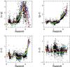 |
Fig. 28 SDSS colors vs. redshift for quasars in the DR9Q catalog. The thin solid red line is the median color in bins of redshift. The thick color lines are models from simulations used to determine the BOSS quasar completeness (McGreer et al., in prep.; see also Ross et al., in prep.) for three different quasar luminosities: Mi [z = 2] = −22.49 (cyan), Mi [z = 2] = −24.99 (green) and Mi [z = 2] = −27.49 (orange); and empirical tracks for the DR7 quasars (blue Bovy et al. 2011). These simulations include the Baldwin effect (Baldwin 1977). Therefore the colors depend on the quasar luminosity. The model is systematically bluer than the data at low redshift because BOSS systematically excludes UV-excess sources. |
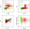 |
Fig. 29 Color–color diagrams for all quasars in the DR9Q catalog. Colors of points encode their redshifts (see top right panel). The stellar locus is represented with black contours. |
7.4. Uniform sample
We provide a similar uniform flag in our catalog to previous versions of the SDSS quasar catalogs (e.g., Schneider et al. 2007). Quasars in our catalog with uniform = 1 are CORE targets that were selected with the XDQSO technique (Bovy et al. 2011) after XDQSO became the CORE targeting algorithm of choice for BOSS (e.g., in or after Chunk 12; Ross et al. 2012). XDQSO will remain the BOSS quasar target algorithm for the rest of the survey, so this uniform = 1 sample will grow significantly in subsequent releases.
Quasars with uniform = 2 would have been selected by XDQSO if it had been the CORE algorithm prior to Chunk 12. uniform = 2 objects are quite complete to what XDQSO would have selected (e.g., Ross et al. 2012), so uniform > 0 is a sufficiently statistical sample for, e.g., clustering measurements on some scales (e.g., White et al. 2012). Quasars in our catalog with uniform = 0 are not homogeneously selected CORE targets. Finally, the very few (30) quasars in our catalog with uniform = -1 have no chunk information, but are a sufficiently small sample to be discarded for the purposes of statistical analyses.
7.5. Multiwavelength matching
7.5.1. ROSAT all sky survey
We cross-correlate the DR9Q catalog with the ROSAT all sky survey catalog listing the sources detected in the energy band 0.1−2.4 keV. The matching radius is set to 30′′.
We report the logarithm of the vignetting-corrected count rate (photons s-1) from the ROSAT All-Sky Survey Faint Source Catalog (Voges et al. 2000) and the ROSAT All-Sky Survey Bright Source Catalog (Voges et al. 1999). An entry of “−9.000” in the column RASS_COUNTS indicates no X-ray detection. We also report the S/N at the position of the quasar and the separation between the quasar and the X-ray source.
There are 16 matches with the Bright Source Catalog and 298 with the Faint Source Catalog. It never happened to find more than one source within the matching radius. No DR9 quasar is detected both in the Bright and Faint Source catalog. Only the most reliable detections were included in our catalog: X-ray counterparts for 13 quasars were flagged for possible detection quality issues and therefore are not included in the present quasar catalog.
7.5.2. The Galaxy Evolution Explorer (GALEX)
The GALEX space mission (Martin et al. 2005) has performed an all-sky imaging survey in two UV bands (FUV: 1350 to 1750 Å; NUV: 1750 to 2750 Å) down to mAB ~ 20.5 and a medium-deep imaging survey that reaches mAB ~ 23 (e.g., Bianchi et al. 2011). Both surveys are used here.
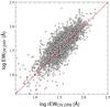 |
Fig. 30 Rest frame equivalent width of the C iv emission line of SDSS-DR7 quasars, measured from the SDSS-DR7 spectra (Shen et al. 2011) and spectra obtained by BOSS (this work). |
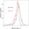 |
Fig. 31 Distribution of the spectral index αν of z > 2 of SDSS-DR7 quasars (red histogram) re-observed by BOSS (black histogram). The spectral index was measured using the rest frame wavelength ranges 1450−1500, 1700−1850 and 1950−2750 Å. As seen already from the composite spectrum shown in Fig. 5, the spectral indices measured using SDSS-DR9 quasar spectra are bluer than those obtained using DR7 spectra (see Sect. 7.2). |
GALEX images are force photometering GALEX images (from GALEX Data Release 5) at the SDSS-DR8 centroids (Aihara et al. 2011), such that low S/N point-spread function (PSF) fluxes of objects not detected by GALEX is obtained.
A total of 77 236 quasars lie in the GALEX FUV footprint, 78 062 lie in the NUV footprint, and 77 197 are covered by both bandpasses.
7.5.3. The two micron all sky survey (2MASS)
We cross-correlate the DR9Q catalog with the All-Sky Data Release Point Source Vatalog (Cutri et al. 2003) using a matching radius of 2.0′′.
Together with the Vega magnitudes in the J, H and K-bands (xMAG with x = J, H or K) and their errors (ERR_xMAG), we report the S/N (xS/N) since the errors on the magnitude do not differentiate the 2σ upper limits (in a 4′′ radius aperture) from detections. We also give for each band the value of the 2MASS flag rd_flg[1] (entry xRDFLAG) which gives the meaning of the peculiar values of xMAG and ERR_xMAG (see http://www.ipac.caltech.edu/2mass/releases/allsky/doc/explsup.html).
There are 1441 matches in the catalog.
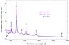 |
Fig. 32 Composite spectra of BOSS quasars in different ranges of absolute magnitude: −25.0 < Mi < −23.5 (magenta), −26.5 < Mi < −25.0 (blue) and Mi < −26.5 (black). All the spectra were normalized to have a flux unity near 1450 Å in the quasar rest frame. The Baldwin effect is apparent (see Table 6). |
7.5.4. The Wide-Field Infrared Survey (WISE)
We take the DR9Q catalog, and match to the Wide-Field Infrared Survey (WISE; Wright et al. 2010) All-Sky Data Release5, asking for all quasars in the DR9Q catalog that are in the All-Sky Source Catalog. WISE photometry covers four bands, 3.4, 4.6, 12 and 22 μm, where the angular resolution of WISE is ≈ 6′′ for 3.4, 4.6, 12 μm, and ≈ 12′′ for 22 μm (Wright et al. 2010). After testing for various matching radii (1′′, 2′′, 6′′, 12′′, 18′′), we use a matching radius of 2.0′′, and a total of 45 987 rows of WISE photometry data are returned, along with the separation in arcseconds between the SDSS and WISE source (stored in SDSSWISE_SEP).
In the DR9Q catalog, we report the photometric quantities, wxmpro, wxsigmpro, wxsnr, wxrchi2, where x = 1−4 and represents the four WISE bands centered at wavelengths of 3.4, 4.6, 12 and 22 μm. These magnitudes are in the Vega system, and are measured with profile-fitting photometry (see e.g. http://wise2.ipac.caltech.edu/docs/release/allsky/expsup/sec2_2a.html and http://wise2.ipac.caltech.edu/docs/release/allsky/expsup/sec4_4c.html#wpro).
Formulae for converting WISE Vega magnitudes to flux density units (in Janskys) and AB magnitudes are given in Wright et al. (2010) and Jarrett et al. (2011) and also here: http://wise2.ipac.caltech.edu/docs/release/allsky/expsup/sec4_4h.html#conv2flux
Although the MIR WISE properties of the BOSS quasars will be valuable for many scientific questions, we strongly urge the user to not only consider the various “health warnings” associated with using the BOSS quasar dataset (as given in Sect. 2) but also those connected to the WISE All-Sky Release Data Products6.
We do not investigate any of the 2MASS, or UKIDSS properties associated with WISE matches here, but these are being investigated in Ross et al. (in prep.).
7.5.5. FIRST
We cross-correlate the DR9Q catalog with objects that are detected in the FIRST radio survey (Becker et al. 1995). We use the version of July 2008.
If there is a source in the FIRST catalog within 2.0′′ of the quasar position, we indicate the FIRST peak flux density and the S/N. Note that extended radio sources may be missed by this matching.
Note that, as in SDSS-I/II, FIRST sources are automatically included in the target selection. An additional cut in color (u − g > 0.4) is added to avoid as much as possible low-redshift sources (Ross et al. 2012). The catalog contains 3283 FIRST matches.
8. Additional quasars
We provide a supplemental list of 949 quasars, of which 318 at z > 2.15, that have been identified among quasar targets after DR9 was “frozen” (Sect. 8.1) or among galaxy targets (Sect. 8.2). This supplemental list of quasars is provided in the same format as the DR9Q catalog but in a separate file and is meant to be merged with the whole catalog for DR10. Figure 33 gives the redshift distribution of these additional quasars. The list is available together with the DR9Q catalog and the list of objects classified as QSO_? at the SDSS public website http://www.sdss3.org/dr9/algorithms/qso_catalog.php
8.1. Additional quasars from the quasar target list
The quasar catalog was frozen7 in February 2012, but we subsequently identified an additional 301 quasars (294 with z > 2.15) that have been targeted as quasar candidates. Some of these were identified with improvements of the pipeline. Others are identified from a good spectrum taken on a plate which was not survey quality so was not included in the first inspection. A handful are objects that have been misidentified during the first inspection but were corrected during the checks.
In addition, a few ancillary programs were not included in the first inspection. Therefore the supplemental list contains the quasars that have been targeted only by these programs. These comprise 500 quasars of which 20 have z > 2.15.
Finally, only objects classified as QSO or QSO_BAL are listed in the official DR9Q catalog. Objects classified as QSO_Z? (126 in total; 122 corresponding to the DR9Q inspection) are also included in the supplemental list. Most of the latter are very peculiar BAL quasars.
8.2. Galaxy targets
In order to be as complete as possible we also tried to identify serendipitous quasars. For this, we visually inspected all objects from the BOSS galaxy target list that the pipeline reliably classifies (ZWARNING = 0) as quasars with z > 2, and all objects classified as GALAXY/BROADLINE. We also visually inspected 10% of the galaxy targets classified as quasars with ZWARNING not equal to zero; none were in fact quasars, so we did not inspect the remaining such objects. A large fraction (65%) of the unclassifiable objects are attributed to the QSO class, but with low significance. They include all sorts of unidentified objects and spectra with calibration problems but probably very few real quasars, if any. In total we identified 22 additional quasars, 4 of which were at z > 2.15, out of more than 3000 targets. There is one quasar classified as QSO_Z?.
9. Conclusion
The quasar catalog presented here contains 87 822 quasars, 61 931 having z > 2.15, with robust identification from visual inspection and redshift derived from the fit of PCA components to the spectra. This catalog has been gathered during the first two years of the BOSS operation covering 3275 deg2. It will be the basis for studies of the luminosity function and the spatial distribution of quasars as well as studies of the clustering properties of the Lyman-α forest. In particular it will be used to measure for the first time the BAO clustering signal in the IGM at z ~ 2.3 from the Lyman-α forest.
For quasars with zem > 1.57, the catalog identifies 7228 broad absorption line quasars from visual inspection, of which 3130 have BI > 500 km s-1. In the 7317 spectra with S/N > 10, we find 813 BALs with BI > 500 km s-1 corresponding to a fraction of 11.1%. We implement a procedure to identify BALs automatically, fitting the quasar continuum with PCAs. 3330 BALs with BI > 500 km s-1 have been identified in this way, of which 821 in spectra of S/N > 10. The catalog gives their characteristics, balnicity and absorption indices. The list of BALs will be used for statistical analysis of this population of quasars. Since SDSS-DR7 z > 2.15 quasars are reobserved by BOSS, this will be a unique opportunity to study the variability of these troughs. High redshift (z > 2) quasar continua together with pixel masks, improved noise estimates, and other products designed to aid in the BAO-Lyman-α clustering analysis will be released in Lee et al. (in prep.).
BOSS is a five year program and the next version of our quasar catalog, to be released as a part of SDSS-DR10 in July 2013, should contain about two times as many quasars as the DR9Q catalog. Improvements in the pipeline will allow us to achieve identification of more objects. We will also perform multiple checks and improve our procedures in order to place better constraints on the characterisitcs of the quasar spectra.
All known z > 2.15 quasars in BOSS footprint are being reobserved to obtain spectra of uniformly high S/N in the Lyman-α forest and to enable variability studies.
The software used is called idlspec2d and is publicly available. The current version is v5_4_45. Details can be found at http://www.sdss3.org/dr9/software, Bolton et al. (2012).
CC-IN2P3, http://cc.in2p3.fr
By which we mean no additional quasar or change in the identifications were intended to be included in the catalog.
Acknowledgments
I.P. received partial support from Center of Excellence in Astrophysics and Associated Technologies (PFB 06). The French Participation Group to SDSS-III was supported by the Agence Nationale de la Recherche under contract ANR-08-BLAN-0222. W.N.B. and N.F.-A. gratefully acknowledge support from NSF AST-1108604. A.D.M. is a research fellow of the Alexander von Humboldt Foundation of Germany. Funding for SDSS-III has been provided by the Alfred P. Sloan Foundation, the Participating Institutions, the National Science Foundation, and the US Department of Energy Office of Science. The SDSS-III web site is http://www.sdss3.org/. SDSS-III is managed by the Astrophysical Research Consortium for the Participating Institutions of the SDSS-III Collaboration including the University of Arizona, the Brazilian Participation Group, Brookhaven National Laboratory, University of Cambridge, Carnegie Mellon University, University of Florida, the French Participation Group, the German Participation Group, Harvard University, the Instituto de Astrofisica de Canarias, the Michigan State/Notre Dame/JINA Participation Group, Johns Hopkins University, Lawrence Berkeley National Laboratory, Max Planck Institute for Astrophysics, Max Planck Institute for Extraterrestrial Physics, New Mexico State University, New York University, Ohio State University, Pennsylvania State University, University of Portsmouth, Princeton University, the Spanish Participation Group, University of Tokyo, University of Utah, Vanderbilt University, University of Virginia, University of Washington, and Yale University.
References
- Abazajian, K. N., Adelman-McCarthy, J. K., Agüeros, M. A., et al. 2009, ApJS, 182, 543 [NASA ADS] [CrossRef] [Google Scholar]
- Ahn, C. P., Alexandroff, R., Allende Prieto, C., et al. 2012, ApJS, submitted [arXiv:1207.7137] [Google Scholar]
- Aihara, H., Allen de Prieto, C., An, D., et al. 2011, ApJS, 193, 29 [NASA ADS] [CrossRef] [Google Scholar]
- Allen, J. T., Hewett, P. C., Maddox, N., Richards, G. T., & Belokurov, V. 2011, MNRAS, 410, 860 [NASA ADS] [CrossRef] [Google Scholar]
- Baldwin, J. A. 1977, ApJ, 214, 679 [NASA ADS] [CrossRef] [Google Scholar]
- Becker, R. H., White, R. L., & Helfand, D. J. 1995, ApJ, 450, 559 [NASA ADS] [CrossRef] [Google Scholar]
- Bentz, M. C., Peterson, B. M., Netzer, H., Pogge, R. W., & Vestergaard, M. 2009, ApJ, 697, 160 [Google Scholar]
- Bianchi, L., Efremova, B., Herald, J., et al. 2011, MNRAS, 411, 2770 [NASA ADS] [CrossRef] [Google Scholar]
- Bolton, A. S., Schlegel, D. J., Aubourg, E., et al. 2012, AJ, 144, 144 [NASA ADS] [CrossRef] [Google Scholar]
- Bovy, J., Hennawi, J. F., Hogg, D. W., et al. 2011, ApJ, 729, 141 [NASA ADS] [CrossRef] [Google Scholar]
- Bovy, J., Myers, A. D., Hennawi, J. F., et al. 2012, ApJ, 749, 41 [NASA ADS] [CrossRef] [Google Scholar]
- Boyle, B. J., Shanks, T., Croom, S. M., et al. 2000, MNRAS, 317, 1014 [NASA ADS] [CrossRef] [Google Scholar]
- Croom, S. M., Shanks, T., Boyle, B. J., et al. 2001, MNRAS, 325, 483 [NASA ADS] [CrossRef] [Google Scholar]
- Croom, S. M., Smith, R. J., Boyle, B. J., et al. 2004, MNRAS, 349, 1397 [NASA ADS] [CrossRef] [Google Scholar]
- Croom, S. M., Richards, F. T., Shanks, T., et al. 2009, MNRAS, 392, 19 [NASA ADS] [CrossRef] [Google Scholar]
- Cutri, R. M., Skrutskie, M. F., van Dyk, S., et al. 2003, VizieR Online Data Catalog II/246 [Google Scholar]
- Dawson, K. S., Schlegel, D. J., Ahn, C. P., et al. 2012, AJ, submitted [arXiv:1208.0022] [Google Scholar]
- Diamond-Stanic, A. M., Fan, X., Brandt, W. N., et al. 2009, ApJ, 699, 782 [NASA ADS] [CrossRef] [Google Scholar]
- Eisenstein, D. J., Weinberg, D. H., Agol, E., et al. 2011, AJ, 142, 72 [Google Scholar]
- Elvis, M., Lockman, F. J., & Fassnacht, C. 1994, ApJS, 95, 413 [NASA ADS] [CrossRef] [EDP Sciences] [Google Scholar]
- Fan, X. 1999, AJ, 117, 2528 [NASA ADS] [CrossRef] [Google Scholar]
- Fan, X., Hennawi, J. F., Richards, G. T., et al. 2004, AJ, 128, 515 [NASA ADS] [CrossRef] [Google Scholar]
- FilizAk, N., Brandt, W. N., Hall, P. B., et al. 2012, ApJ, 757, 114 [NASA ADS] [CrossRef] [Google Scholar]
- Font-Ribera, A., Miralda-Escudé, J., Arnau, E., et al. 2012, J. Cosmology Astropart. Phys. [arXiv:1209.4596] [Google Scholar]
- Francis, P. J., Hewett, P. C., Foltz, C. B., & Chaffee, F. H. 1992, ApJ, 398, 476 [NASA ADS] [CrossRef] [Google Scholar]
- Fukugita, M., Ichikawa, T., Gunn, J. E., et al. 1996, AJ, 111, 1748 [NASA ADS] [CrossRef] [Google Scholar]
- Gaskell, C. M. 1982, ApJ, 263, 79 [NASA ADS] [CrossRef] [Google Scholar]
- Gibson, R. R., Brandt, W. N., Schneider, D. P., & Gallagher, S. C. 2008, ApJ, 675, 985 [NASA ADS] [CrossRef] [Google Scholar]
- Gibson, R. R., Jiang, L., Brandt, W. N., et al. 2009, ApJ, 692, 758 [NASA ADS] [CrossRef] [Google Scholar]
- Gibson, R. R., Brandt, W. N., Gallagher, S. C., Hewett, P. C., & Schneider, D. P. 2010, ApJ, 713, 220 [NASA ADS] [CrossRef] [Google Scholar]
- Gunn, J. E., Carr, M., Rockosi, C., et al. 1998, AJ, 116, 3040 [NASA ADS] [CrossRef] [Google Scholar]
- Gunn, J. E., Siegmund, W. A., Mannery, E. J., et al. 2006, AJ, 131, 2332 [NASA ADS] [CrossRef] [Google Scholar]
- Hall, P. B., Anderson, S. F., Strauss, M. A., et al. 2002, ApJS, 141, 267 [NASA ADS] [CrossRef] [Google Scholar]
- Hennawi, J. F., Myers, A. D., Shen, Y., et al. 2010, ApJ, 719, 1672 [NASA ADS] [CrossRef] [Google Scholar]
- Hewett, P. C., & Wild, V. 2010, MNRAS, 405, 2302 (HW10) [NASA ADS] [Google Scholar]
- Hewett, P. C., Foltz, C. B., & Chaffee, F. H. 1995, AJ, 109, 1498 [NASA ADS] [CrossRef] [Google Scholar]
- Hewitt, A., & Burbidge, G. 1993, ApJS, 87, 451 [NASA ADS] [CrossRef] [Google Scholar]
- Hogg, D. W., Finkbeiner, D. P., Schlegel, D. J., & Gunn, J. E. 2001, AJ, 122, 2129 [NASA ADS] [CrossRef] [Google Scholar]
- Ivezić, Ž., Lupton, R. H., Schlegel, D., et al. 2004, Astron. Nachr., 325, 583 [NASA ADS] [CrossRef] [Google Scholar]
- Jarrett, T. H., Cohen, M., Masci, F., et al. 2011, ApJ, 735, 112 [NASA ADS] [CrossRef] [Google Scholar]
- Kaspi, S., Brandt, W. N., George, I. M., et al. 2002, ApJ, 574, 643 [NASA ADS] [CrossRef] [Google Scholar]
- Kirkpatrick, J. A., Schlegel, D. J., Ross, N. P., et al. 2011, ApJ, 743, 125 [NASA ADS] [CrossRef] [Google Scholar]
- Lawrence, A., Warren, S. J., Almaini, O., et al. 2007, MNRAS, 379, 1599 [NASA ADS] [CrossRef] [MathSciNet] [Google Scholar]
- Lupton, R., Gunn, J. E., Ivezić, Z., et al. 2001, in Astronomical Data Analysis Software and Systems X, eds. F. R. Harnden Jr., F. A. Primini, & H. E. Payne, ASP Conf. Ser., 238, 269 [Google Scholar]
- MacLeod, C., Butler, N., Anderson, S. F., et al. 2012, in AAS Meeting Abstracts, 219, 243.28 [Google Scholar]
- Martin, D. C., Fanson, J., Schiminovich, D., et al. 2005, ApJ, 619, L1 [Google Scholar]
- McDonald, P., & Eisenstein, D. J. 2007, Phys. Rev. D, 76, 063009 [NASA ADS] [CrossRef] [Google Scholar]
- McIntosh, D. H., Rix, H.-W., Rieke, M. J., & Foltz, C. B. 1999, ApJ, 517, L73 [NASA ADS] [CrossRef] [Google Scholar]
- Morris, S. L., Weymann, R. J., Anderson, S. F., et al. 1991, AJ, 102, 1627 [NASA ADS] [CrossRef] [Google Scholar]
- Noterdaeme, P., Petitjean, P., Ledoux, C., & Srianand, R. 2009, A&A, 505, 1087 [NASA ADS] [CrossRef] [EDP Sciences] [Google Scholar]
- Noterdaeme, P., Petitjean, P., Carithers, W. C., et al. 2012, A&A, 547, L1 [NASA ADS] [CrossRef] [EDP Sciences] [Google Scholar]
- Padmanabhan, N., Schlegel, D. J., Finkbeiner, D. P., et al. 2008, ApJ, 674, 1217 [NASA ADS] [CrossRef] [MathSciNet] [Google Scholar]
- Palanque-Delabrouille, N., Yèche, C., Myers, A. D., et al. 2011, A&A, 530, A122 [NASA ADS] [CrossRef] [EDP Sciences] [Google Scholar]
- Palanque-Delabrouille, N., Magneville, C., Yeche, C., et al. 2012, A&A, submitted [arXiv:1209.3968] [Google Scholar]
- Pâris, I., Petitjean, P., Rollinde, E., et al. 2011, A&A, 530, A50 [NASA ADS] [CrossRef] [EDP Sciences] [Google Scholar]
- Peth, M. A., Ross, N. P., & Schneider, D. P. 2011, AJ, 141, 105 [NASA ADS] [CrossRef] [Google Scholar]
- Pier, J. R., Munn, J. A., Hindsley, R. B., et al. 2003, AJ, 125, 1559 [NASA ADS] [CrossRef] [Google Scholar]
- Prochaska, J. X., Worseck, G., & O’Meara, J. M. 2009, ApJ, 705, L113 [NASA ADS] [CrossRef] [Google Scholar]
- Richards, G. T., Fan, X., Newberg, H. J., et al. 2002, AJ, 123, 2945 [NASA ADS] [CrossRef] [Google Scholar]
- Richards, G. T., Hall, P. B., Van den Berk, D. E., et al. 2003, AJ, 126, 1131 [NASA ADS] [CrossRef] [Google Scholar]
- Richards, G. T., Nichol, R. C., Gray, A. G., et al. 2004, ApJS, 155, 257 [NASA ADS] [CrossRef] [Google Scholar]
- Richards, G. T., Strauss, M. A., Fan, X., et al. 2006, AJ, 131, 2766 [NASA ADS] [CrossRef] [Google Scholar]
- Richards, G. T., Myers, A. D., Gray, A. G., et al. 2009, ApJS, 180, 67 [NASA ADS] [CrossRef] [Google Scholar]
- Ross, N. P., Myers, A. D., Sheldon, E. S., et al. 2012, ApJS, 199, 3 [NASA ADS] [CrossRef] [Google Scholar]
- Schlafly, E. F., & Finkbeiner, D. P. 2011, ApJ, 737, 103 [NASA ADS] [CrossRef] [Google Scholar]
- Schlegel, D. J., Finkbeiner, D. P., & Davis, M. 1998, ApJ, 500, 525 [NASA ADS] [CrossRef] [Google Scholar]
- Schlegel, D. J., Blanton, M., Eisenstein, D., et al. 2007, in BAAS, 38, 966 [Google Scholar]
- Schmidt, M. 1963, Nature, 197, 1040 [NASA ADS] [CrossRef] [Google Scholar]
- Schneider, D. P., Richards, G. T., Fan, X., et al. 2002, AJ, 123, 567 [NASA ADS] [CrossRef] [Google Scholar]
- Schneider, D. P., Fan, X., Hall, P. B., et al. 2003, AJ, 126, 2579 [NASA ADS] [CrossRef] [Google Scholar]
- Schneider, D. P., Hall, P. B., Richards, G. T., et al. 2005, AJ, 130, 367 [NASA ADS] [CrossRef] [Google Scholar]
- Schneider, D. P., Hall, P. B., Richards, G. T., et al. 2007, AJ, 134, 102 [NASA ADS] [CrossRef] [Google Scholar]
- Schneider, D. P., Richards, G. T., Hall, P. B., et al. 2010, AJ, 139, 2360 [NASA ADS] [CrossRef] [Google Scholar]
- Shang, Z., Wills, B. J., Wills, D., & Brotherton, M. S. 2007, AJ, 134, 294 [NASA ADS] [CrossRef] [Google Scholar]
- Shen, Y., Strauss, M. A., Oguri, M., et al. 2007, AJ, 133, 2222 [NASA ADS] [CrossRef] [Google Scholar]
- Shen, Y., Greene, J. E., Strauss, M. A., Richards, G. T., & Schneider, D. P. 2008, ApJ, 680, 169 [NASA ADS] [CrossRef] [Google Scholar]
- Shen, Y., Richards, G. T., Strauss, M. A., et al. 2011, ApJS, 194, 45 [NASA ADS] [CrossRef] [Google Scholar]
- Smee, S., Gunn, J. E., Uomoto, A., et al. 2012, AJ, submitted [arXiv:1208.2233] [Google Scholar]
- Smith, J. A., Tucker, D. L., Kent, S., et al. 2002, AJ, 123, 2121 [Google Scholar]
- Spergel, D. N., Verde, L., Peiris, H. V., et al. 2003, ApJS, 148, 175 [NASA ADS] [CrossRef] [Google Scholar]
- Stark, A. A., Gammie, C. F., Wilson, R. W., et al. 1992, ApJS, 79, 77 [NASA ADS] [CrossRef] [Google Scholar]
- Stoughton, C., Lupton, R. H., Bernardi, M., et al. 2002, AJ, 123, 485 [NASA ADS] [CrossRef] [Google Scholar]
- Suzuki, N., Tytler, D., Kirkman, D., O’Meara, J. M., & Lubin, D. 2005, ApJ, 618, 592 [NASA ADS] [CrossRef] [Google Scholar]
- Trump, J. R., Hall, P. B., Reichard, T. A., et al. 2006, ApJS, 165, 1 [NASA ADS] [CrossRef] [Google Scholar]
- Tucker, D. L., Kent, S., Richmond, M. W., et al. 2006, Astron. Nachr., 327, 821 [NASA ADS] [CrossRef] [Google Scholar]
- Vanden Berk, D. E., Richards, G. T., Bauer, A., et al. 2001, AJ, 122, 549 [NASA ADS] [CrossRef] [Google Scholar]
- Véron-Cetty, M.-P., & Véron, P. 2006, A&A, 455, 773 [NASA ADS] [CrossRef] [EDP Sciences] [Google Scholar]
- Voges, W., Aschenbach, B., Boller, T., et al. 1999, A&A, 349, 389 [NASA ADS] [Google Scholar]
- Voges, W., Aschenbach, B., Boller, T., et al. 2000, IAU Circ., 7432, 3 [NASA ADS] [Google Scholar]
- Weymann, R. J., Morris, S. L., Foltz, C. B., & Hewett, P. C. 1991, ApJ, 373, 23 [NASA ADS] [CrossRef] [Google Scholar]
- White, M., Myers, A. D., Ross, N. P., et al. 2012, MNRAS, 424, 933 [NASA ADS] [CrossRef] [Google Scholar]
- Wilhite, B. C., Van den Berk, D. E., Brunner, R. J., & Brinkmann, J. V. 2006, ApJ, 641, 78 [NASA ADS] [CrossRef] [Google Scholar]
- Worseck, G., & Prochaska, J. X. 2011, ApJ, 728, 23 [NASA ADS] [CrossRef] [Google Scholar]
- Wright, E. L., Eisenhardt, P. R. M., Mainzer, A. K., et al. 2010, AJ, 140, 1868 [NASA ADS] [CrossRef] [Google Scholar]
- Yèche, C., Petitjean, P., Rich, J., et al. 2010, A&A, 523, A14 [NASA ADS] [CrossRef] [EDP Sciences] [Google Scholar]
- Yip, C. W., Connolly, A. J., Van den Berk, D. E., et al. 2004, AJ, 128, 2603 [NASA ADS] [CrossRef] [Google Scholar]
- York, D. G., Adelman, J., Anderson, Jr., J. E., et al. 2000, AJ, 120, 1579 [Google Scholar]
All Tables
Classification from the visual inspection corresponding to the combination of class_person (first column) and z_conf_person (first row) values provided in the headers of the SDSS-DR9 spectra available from the SDSS Catalog Archive Server.
Number of objects identified as such by the pipeline with any ZWARNING value (second column) and with ZWARNING = 0 (third column), and after the visual inspection (fourth column).
Number of visually inspected DR9 BOSS quasar targets (third column) and identifications in the DR9Q catalog for each target selection method (first column; see Table 4 of Ross et al. 2012, and Tables 6 and 7 in the Appendix of Dawson et al. 2012).
All Figures
|
Fig. 1 The space distribution in equatorial coordinates of the SDSS-III DR9 data release quasars. |
| In the text | |
|
Fig. 2 Cumulative number of quasars as a function of observation date during the first two years of the survey. Horizontal times are due to the yearly summer shutdown during monsoon rains (summer 2010 at MJD = 55 400) and the monthly bright time when BOSS does not observe. |
| In the text | |
|
Fig. 3 Median observed S/N per pixel at the top of the Lyman-α (green), C iv (red), C iii] complex (blue), Mg ii at z > 2 (orange) and Mg ii at z < 2 (yellow) emission lines and in emission-line free regions (black) versus r-PSF magnitude (corrected for Galactic extinction). Two redshift ranges are considered for Mg ii because the emission line is redshifted in regions of the spectra with very different characteristics. At r ~ 22, the median S/N per pixel at the top of the Lyman-α and C iv emission lines is about 4; sufficient to identify most of the quasars. Outside of the emission-line regions, at the same magnitude, the S/N per pixel is about unity. |
| In the text | |
|
Fig. 4 Stack of DR9 BOSS spectra where a damped Lyman-α system is seen at an absorpstion redshift higher than 3.385 with a column density N(H i) ≥ 1020.5 cm-2. The spectra are normalized to unity near 1280 Å in the quasar rest frame. Owing to the presence of the DLA, the flux is expected to be zero at observed wavelengths below ~4100 Å (e.g. below the Lyman limit of all DLAs). This is not the case in the very blue part of the spectrum (λobs ≤ 4000 Å) where the mean observed flux appears to increase (spuriously). |
| In the text | |
|
Fig. 5 Composite spectra of 6459 quasars observed both by SDSS-DR7 and BOSS for (i) SDSS-DR7 spectra (red) and; (ii) SDSS-DR9 spectra (black). The slope of the two composite spectra should be similar (as any variability should be averaged out). This is not the case because of the difference in focus of the BOSS quasars and standard stars. Note that this flux mis-calibration is different from object to object. |
| In the text | |
|
Fig. 6 Fraction of visually confirmed quasars with a non-zero ZWARNING flag as a function of the r-PSF magnitude (after correcting for Galactic extinction). A positive ZWARNING means that the pipeline considers its redshift estimate to be unreliable. This fraction increases at faint magnitudes. |
| In the text | |
|
Fig. 7 First column: examples of z > 2 quasars classified as STAR by the BOSS pipeline. The overall shape of the spectrum is similar to the spectrum of F stars. Second column: examples of stars identified as QSO by the BOSS pipeline. Strong absorption lines or wiggles in the spectrum can mimic quasar features. Third colum: examples of z > 2 quasars for which the BOSS pipeline provides an inaccurate redshift estimate that must be corrected during the visual inspection. The pipeline is confused by the strong absorption lines. The spectra were boxcar median smoothed over 5 pixels. |
| In the text | |
|
Fig. 8 Examples of QSO_? (top panels) and QSO_Z? (lower panels). The spectra were boxcar median smoothed over 5 pixels. |
| In the text | |
|
Fig. 9 Normalized (to unit integral) distribution of the velocity difference between the pipeline and visual inspection redshift estimates for different redshift bins. About half of the pipeline redshifts are corrected during the visual inspection. Most of the corrections are for quasars with 2 < z < 2.5 where the Mg ii emission line is available and where the pipeline redshift estimate does not correspond to the peak of the Mg ii emission line. |
| In the text | |
|
Fig. 10 H i column density distribution for DLAs and sub-DLAs detected by Noterdaeme et al. (2009) in quasars observed both by SDSS-DR7 and BOSS (black histogram). The red histogram displays the same distribution but for DLAs flagged after visual inspection of BOSS spectra. This shows that the visual inspection is robust for log N(H i) > 20.3, the standard definition of DLAs. |
| In the text | |
|
Fig. 11 Mean spectrum and the first five principal components derived in Sect. 4.2. A linear combination of the first four principal components is used to estimate the global redshift of the quasar, while five components are used to fit emission lines locally. |
| In the text | |
|
Fig. 12 Distributions of the velocity difference between PCA redshift estimates derived using different rest frame wavelength ranges and the PCA Mg ii redshift estimate. |
| In the text | |
|
Fig. 13 Normalized distributions of the velocity difference between our global PCA redshift estimate (black histogram), the pipeline redshift estimate (blue histogram) or Hewett & Wild (2010) redshifts (red histogram) with the redshift derived from a PCA fit of the Mg ii emission line (see text). |
| In the text | |
|
Fig. 14 Velocity difference between C iv and Mg ii emission line redshifts as a function of the absolute i magnitude of the quasar. The solid black line shows the median velocity shift in 0.2 mag bins. Blue and cyan histograms display the 10th, 30th, 70th and 90th percentiles. The mean shift between the two emission lines increases with the quasar luminosity. |
| In the text | |
|
Fig. 15 Examples of high-redshift BAL quasar spectra in different ranges of S/N and BI. The fit of the continuum is overplotted. |
| In the text | |
|
Fig. 16 Ratio of the numbers of BAL visual and automatic detections as a function of spectral S/N per pixel at λrest = 1700 Å for BI > 500 km s-1. As expected, this ratio decreases with decreasing S/N. |
| In the text | |
|
Fig. 17 Distribution of BI and AI for quasars detected as BAL by automatic procedures in previous SDSS releases, and that were not flagged by the visual inspection of the BOSS spectra. The black histogram shows the distribution of AI as measured by Trump et al. (2006) for 296 such quasars (all have BI = 0). About half of them are not real BALs (see text). From the automatic detection by Allen et al. (2011) (blue histogram), 57 quasars were missed by the visual inspection. Here again, only a handful of these objects actually display BAL troughs. |
| In the text | |
|
Fig. 18 Example of appearing BAL troughs. This quasar has been observed in SDSS-DR7 (red curve) and in SDSS-DR9 (black curve). The two spectra have been scaled to have a surface unity between 5600 and 6200 Å. The normalized flux in the C iv region expressed in velocity is displayed in the inset. This quasar had was not detected as BAL in SDSS-DR7 (i.e. BI = 0) while it has BI = 1826 km s-1 in the SDSS-DR9 spectrum. |
| In the text | |
|
Fig. 19 Normalized distributions of the logarithm of BI measured from C iv troughs. The BI distribution from the present catalog (black histogram) computed from 7227 visually flagged BAL quasars is very similar to the distribution from Trump et al. (2006, red histogram) obtained from 1102 BAL quasars from the SDSS-DR3 quasar catalog (Schneider et al. 2005). The distribution is also very similar to the BI distribution from Allen et al. (2011, blue histogram) based on the SDSS-DR6 quasar catalog. |
| In the text | |
|
Fig. 20 Balnicity index (BI) from this work against BI measured by Allen et al. (2011) for SDSS-DR6 objects re-observed by BOSS. |
| In the text | |
|
Fig. 21 Left panel: distribution of AI from our automatic detection (black histogram) and from SDSS-DR3 (red histogram, Trump et al. 2006). The distributions are normalized for log AI > 3. The difference between the two results at low AI is a consequence of slightly different formula used to measure AI. Right panel: distribution of BI from our automatic detection (black histogram) and from SDSS-DR6 (blue histogram, Allen et al. 2011). |
| In the text | |
|
Fig. 22 The redshift distribution of quasars from this catalog is displayed in black. The same distribution is shown for newly discovered quasars only (dashed blue histogram). Most of the SDSS-DR9 quasars have a redshift greater than 2. The redshift distribution of quasars from the SDSS-DR7 catalog (Schneider et al. 2010) is shown for comparison in red. The latter is dominated by quasars at low redshift. The present catalog contains 2.6 times more quasars at z > 2.15 than the DR7 catalog. |
| In the text | |
|
Fig. 23 Redshift distribution of SDSS-DR9 quasars in the range 2.00−4.00 for the whole distribution (black histogram), the CORE sample (red histogram) and the BONUS sample (blue histogram). The CORE sample was uniformly selected through the likelihood method (Kirkpatrick et al. 2011) during most of the first year of operation and the XDQSO method (Bovy et al. 2011) for the second year. The BONUS sample was selected through a combination of four target selection algorithms to maximize the number of high-redshift quasars in the sample. |
| In the text | |
|
Fig. 24 First row, left: spectrum of the highest redshift quasar (z = 5.855) observed by BOSS; this quasar was discovered by Fan et al. (2004); the quasar with highest redshift discovered by BOSS is SDSS J222018.50−010147.0 at z = 5.605. First row, right: spectrum of the most luminous (Mi[z = 2] = −30.91) quasar available in this catalog. Middle and bottom rows: four typical quasar spectra selected to be representative in terms of S/N at different redshifts (z ~ 2.3, 2.5, 2.7, 3.5). The S/N listed is the median S/N per pixel over the whole spectrum. All the spectra were boxcar median smoothed over 5 pixels. |
| In the text | |
|
Fig. 25 Top panel: distribution of r magnitude of SDSS-DR9 quasars (PSF; corrected for Galactic extinction). Bottom panel: median S/N per pixel over the whole spectrum with respect to the r-PSF magnitude (black histogram). Percentiles are indicated in grey. |
| In the text | |
|
Fig. 26 Fraction of quasar candidates confirmed as quasars (red histogram) and z > 2.15 quasars (blue histogram) versus the i-band PSF magnitude (corrected for Galactic extinction). |
| In the text | |
|
Fig. 27 L − z plane for SDSS-DR9 quasars (black contours and points) and SDSS-DR7 quasars (red contours and points; Schneider et al. 2010). The luminosity assumes H0 = 70 km s-1 Mpc-1 and the K-correction is given by Richards et al. (2006) who consider K(z = 2) = 0. Contours are drawn at constant point density. |
| In the text | |
|
Fig. 28 SDSS colors vs. redshift for quasars in the DR9Q catalog. The thin solid red line is the median color in bins of redshift. The thick color lines are models from simulations used to determine the BOSS quasar completeness (McGreer et al., in prep.; see also Ross et al., in prep.) for three different quasar luminosities: Mi [z = 2] = −22.49 (cyan), Mi [z = 2] = −24.99 (green) and Mi [z = 2] = −27.49 (orange); and empirical tracks for the DR7 quasars (blue Bovy et al. 2011). These simulations include the Baldwin effect (Baldwin 1977). Therefore the colors depend on the quasar luminosity. The model is systematically bluer than the data at low redshift because BOSS systematically excludes UV-excess sources. |
| In the text | |
|
Fig. 29 Color–color diagrams for all quasars in the DR9Q catalog. Colors of points encode their redshifts (see top right panel). The stellar locus is represented with black contours. |
| In the text | |
|
Fig. 30 Rest frame equivalent width of the C iv emission line of SDSS-DR7 quasars, measured from the SDSS-DR7 spectra (Shen et al. 2011) and spectra obtained by BOSS (this work). |
| In the text | |
|
Fig. 31 Distribution of the spectral index αν of z > 2 of SDSS-DR7 quasars (red histogram) re-observed by BOSS (black histogram). The spectral index was measured using the rest frame wavelength ranges 1450−1500, 1700−1850 and 1950−2750 Å. As seen already from the composite spectrum shown in Fig. 5, the spectral indices measured using SDSS-DR9 quasar spectra are bluer than those obtained using DR7 spectra (see Sect. 7.2). |
| In the text | |
|
Fig. 32 Composite spectra of BOSS quasars in different ranges of absolute magnitude: −25.0 < Mi < −23.5 (magenta), −26.5 < Mi < −25.0 (blue) and Mi < −26.5 (black). All the spectra were normalized to have a flux unity near 1450 Å in the quasar rest frame. The Baldwin effect is apparent (see Table 6). |
| In the text | |
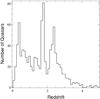 |
Fig. 33 Redshift distribution of the 949 additional quasars described in Sect. 8. |
| In the text | |
Current usage metrics show cumulative count of Article Views (full-text article views including HTML views, PDF and ePub downloads, according to the available data) and Abstracts Views on Vision4Press platform.
Data correspond to usage on the plateform after 2015. The current usage metrics is available 48-96 hours after online publication and is updated daily on week days.
Initial download of the metrics may take a while.