| Issue |
A&A
Volume 548, December 2012
|
|
|---|---|---|
| Article Number | A108 | |
| Number of page(s) | 14 | |
| Section | Extragalactic astronomy | |
| DOI | https://doi.org/10.1051/0004-6361/201219554 | |
| Published online | 30 November 2012 | |
Comparison of the VIMOS-VLT Deep Survey with the Munich semi-analytical model
II. The colour − density relation up to z ~ 1.5
1 INAF – Osservatorio Astronomico di Trieste, via Tiepolo 11, 34143 Trieste Italy
e-mail: This email address is being protected from spambots. You need JavaScript enabled to view it.
2 INAF – Osservatorio Astronomico di Bologna, via Ranzani 1, 40127 Bologna, Italy
3 INAF – Osservatorio Astronomico di Brera, via Brera 28, 20021 Milan, Italy
4 SUPA, Institute for Astronomy, University of Edinburgh, Royal Observatory, Blackford Hill, EH9 3 HJ Edinburgh, UK
5 Centre de Recherche Astrophysique de Lyon, UMR 5574, Université Claude Bernard Lyon-École Normale Supérieure de Lyon-CNRS, 69230 Saint-Genis Laval, France
6 INAF – IASFBO, via P. Gobetti 101, 40129 Bologna, Italy
7 Aix Marseille Université, CNRS, LAM (Laboratoire d’Astrophysique de Marseille) UMR 7326, 13388 Marseille, France
8 The Andrzej Soltan Institute for Nuclear Studies, ul. Hoza 69, 00-681 Warszawa, Poland
9 Astronomical Observatory of the Jagiellonian University, ul. Orla 171, 30-244 Kraków, Pola
Received: 7 May 2012
Accepted: 7 September 2012
Abstract
Aims. Our aim is to perform the same colour − density analysis on galaxy mock samples as was carried out on a 5 h-1 Mpc scale using the VIMOS-VLT Deep Survey (VVDS), and to compare the results from these mock samples with observed data. This allows us to test galaxy evolution in the model and to understand the relation between the studied environment and the underlying dark matter distribution.
Methods. We used galaxy mock catalogues with the same flux limits as the VVDS-Deep (IAB ≤ 24) survey (Cmocks), constructed using a semi-analytic model for galaxy evolution applied to the Millennium Simulation. From each Cmock, we extracted a sub-sample of galaxies mimicking the VVDS observational strategy (Omocks). We then computed the B-band luminosity function LF and the colour − density relation in the mock samples using the same methods as employed for the VVDS data.
Results. We find that the B-band LF in mock samples roughly agrees with the observed LF, but at 0.2 < z < 0.8 the faint-end slope of the model LF is steeper than the observed one. Computing the LF for early- and late-type galaxies separately, we show that mock samples have an excess of faint early-type galaxies and of bright late-type galaxies compared with the data. We find that the colour − density relation in Omocks agrees excellently with that in Cmocks. This suggests that the VVDS observational strategy does not introduce any severe bias to the observed colour − density relation. At z ~ 0.7, the colour − density relation in mock samples agrees qualitatively with observations, with red galaxies residing preferentially in high densities. However, the strength of the colour − density relation in mock samples does not vary within 0.2 < z < 1.5, while the observed relation flattens with increasing redshift and possibly inverts at z ~ 1.3. We argue that the lack of evolution in the colour − density relation in the model cannot be due only to inaccurate prescriptions for the evolution of satellite galaxies, but indicates that the treatment of the central galaxies has also to be revised.
Conclusions. The reversal of the colour − density relation can be explained by wet mergers between young galaxies, producing a starburst event. This should be seen on group scales, where mergers are frequent, with possibly some residual trend on larger scales. This residual is found in observations at z = 1.5 on a scale of ~5 h-1 Mpc, but not in the model, suggesting that the treatment of physical processes influencing both satellites and central galaxies in models should be revised. A detailed analysis would be desirable on small scales as well, which requires flux limits fainter than those of the VVDS data.
Key words: galaxies: evolution / galaxies: fundamental parameters / galaxies: luminosity function, mass function / cosmology: observations / large-scale structure of Universe / galaxies: high-redshift
© ESO, 2012
1. Introduction
Several physical mechanisms are expected to influence the properties of galaxies in overdense regions: ram pressure stripping of gas (Gunn & Gott 1972), galaxy-galaxy merging (Toomre & Toomre 1972), strangulation (Larson et al. 1980), and harassment (Farouki & Shapiro 1981; Moore et al. 1996). Each mechanism has specific environmental dependencies and timescales, but their relative role in regulating galaxy formation and determining the observed trends remains unclear. In addition, it is not yet clear to what extent internal processes such as feedback from supernovae and central black holes contribute to the observed environmental dependence of the galaxy structural parameters. Finally, it is known that in a Gaussian random field there is a statistical correlation between mass fluctuations on different scales, with most massive halos preferentially residing within large-scale overdensities (see Kaiser 1987; Mo & White 1996). The role of initial cosmological conditions in modulating the observed density dependence of galaxy properties is less clear (Abbas & Sheth 2005).
Semi-analytical models (SAMs) of galaxy formation coupled with dark matter (DM) simulations provide a useful tool to address these questions. In SAMs, the individual physical processes taking place during galaxy evolution are expressed through simple equations that are motivated by observational and/or theoretical studies. These equations parametrise the dependency of these processes on physical properties of galaxies and/or those of the dark matter haloes in which they reside. Then, the comparison between galaxy properties in SAMs and in the observed data gives important feedback on the validity of the prescriptions used in the models and on the nature of the observed correlation between galaxy properties and environment. Models are usually tuned to reproduce some (sub)set of observational data in the local Universe, most notably the observed local galaxy luminosity function (LF) and/or mass function. Tracing galaxy evolutionary paths back in time, pushing these studies at high redshifts, becomes thus a very powerful tool in terms of distinguishing between different models.
The recent completion of large and deep high-redshift surveys makes a detailed comparison between model predictions and observational data possible (see e.g. Stringer et al. 2009; de la Torre et al. 2011). Following galaxy evolution over a wide redshift range can help addressing the open question of the apparent contradiction between the hierarchical growth of DM structures and the “downsizing” scenario of luminous matter. A number of different observational tests support a “hierarchical” scenario for structure formation in which DM halos form first in the highest density peaks of the primordial density field, and then grow hierarchically through subsequent mergers (e.g. Peebles 1980). Observations have shown that galaxy evolution does not proceed in a similar “bottom-up” fashion, at least for their star formation (SF) histories: with increasing cosmic time, SF moves towards less massive galaxies (Cowie et al. 1996; Gavazzi et al. 1996). As discussed in e.g. De Lucia et al. (2006), these findings are not necessarily evidence of “anti-hierarchical” growth of luminous matter because the “formation” of the galaxy stellar population does not coincide with its assembly (see Fontanot et al. 2009, for a more detailed discussion about different manifestations of downsizing and comparison with observational data).
Simulations can also help in clarifying the relation between different definitions that are commonly adopted for the “environment”. Indeed, different quantities have been used in the literature to characterise the local and/or global environment. The use of different environmental definitions makes it very difficult to compare results from different surveys, and at different cosmic epochs. Using simulated galaxy samples allow us to have a common reference for the environment, such as the underlying DM distribution.
In this paper, we use mock galaxy samples constructed from semi-analytic models applied to the Millennium Simulation1 (Springel et al. 2005) to carry out a detailed comparison with the observational results presented in Cucciati et al. (2006, C06 hereafter), based on the VIMOS-VLT Deep Survey (VVDS, see Le Fèvre et al. 2005). A detailed comparison between observations and model data for galaxy number counts, redshift and colour distribution, and galaxy clustering was presented in de la Torre et al. (2011, Paper I hereafter). Here we focus on the observed colour − density relation and its evolution.
The aims of our study are (i) to test the robustness of observational results in C06 versus possible biases owing to the respective observational strategy (e.g., does the VVDS sampling rate alter the strength of the colour − density relation?); (ii) to test galaxy evolution in mock samples (do we see the same environmental effects on galaxy properties in the model and observed data?); (iii) to understand which “environment” is being studied (e.g., what is the relation between the density traced by galaxies and the underlying DM distribution?).
This paper is organised as follows. Section 2 gives a summary of the VVDS data used in C06 and describes the mock galaxy samples used for the model comparison. In Sect. 3, we compare the rest-frame B-band LF of the VVDS data with that obtained using mock samples. Section 4 describes the local density and colour distributions in mock samples and compares the colour − density relation in C06 with that found in the model. In Sect. 5 we take advantage of the available mock samples to analyse how the local density computed on a 5 h-1 Mpc scale compares with the total halo mass in which galaxies reside. In Sect. 6 we discuss our results, and we summarise them in Sect. 7.
Throughout this paper, we use the AB flux normalisation for both observed data and mock samples. When we refer to observed data, we adopt the concordance cosmology (Ωm, ΩΛ, h) = (0.3, 0.7, 0.7).
2. Data and mock samples
2.1. The VVDS Deep sample
The VVDS is a large spectroscopic survey with the primary aim of studying galaxy evolution and large-scale structure formation over the redshift range 0 < z < 5. Details on the survey strategy are described in Le Fèvre et al. (2005). The VVDS is complemented by ancillary deep photometric data: BVRI from the CFHT-12K camera (McCracken et al. 2003; Le Fèvre et al. 2004), JK from the NTT telescope (Iovino et al. 2005; Temporin et al. 2008), U from the MPI telescope (Radovich et al. 2004), u∗, g′, r′, i′, z′-band data from the CFHT Legacy Survey and JHKS from the WIRDS survey (Bielby et al. 2012) with the CFHT-WIRCAM camera (see Cucciati et al. 2012, for a detailed description).
This paper is based on the colour − density relation studied in C06, over the VVDS-0226-04 Deep field (from now on “VVDS-02h field”). We refer the reader to that paper for a detailed description of the data. Briefly, the VVDS-02h data set is a purely flux-limited spectroscopic sample, with 17.5 ≤ IAB ≤ 24.0. In this range of magnitudes, the parent photometric catalogue is complete and free from surface brightness selection effects (McCracken et al. 2003). Spectroscopic observations were carried out at the ESO-VLT with the VIsible Multi-Object Spectrograph (VIMOS) using the LRRed grism. The rms accuracy of the redshift measurements is ~275 km s-1 (Le Fèvre et al. 2005). The VVDS-02h field covers a total area of 0.7 × 0.7 deg2, targeted by 1, 2 or 4 spectrograph passes, and it probes a comoving volume (up to z = 1.5) of nearly 1.5 × 10⁶ h-3 Mpc3 in a standard ΛCDM cosmology. The covered field has transversal dimensions ~37 × 37 h-1 Mpc at z = 1.5. Averaging over the area observed, spectra were obtained for a total of 22.8% of the photometric sources, and ~80% of these targeted objects yield a reliable redshift, resulting in an overall sampling rate of ~18% (see Ilbert et al. 2005). The final galaxy sample used in C06 contains 6582 galaxies with reliable redshifts.
2.2. The mock samples
Mock galaxy samples were obtained by applying the semi-analytical model of galaxy evolution described in De Lucia & Blaizot (2007) to the dark matter halo merging trees derived from the Millennium Simulation (Springel et al. 2005). This contains N = 21603 particles of mass 8.6 × 10⁸ h-1 M⊙ within a comoving box of size 500 h-1 Mpc on a side. The adopted cosmological model is a ΛCDM model with Ωm = 0.25, Ωb = 0.045, h = 0.73, ΩΛ = 0.75, n = 1, and σ8 = 0.9.
The semi-analytical model used here is fully described in De Lucia & Blaizot (2007). It builds on results from previous works (Kauffmann & Haehnelt 2000; Springel et al. 2001; De Lucia et al. 2004; Croton et al. 2006) to describe the relevant physical processes, e.g. star formation, gas accretion and cooling, formation of super-massive black holes and galaxy mergers, feedback (also “radio mode” feedback). The SAM model used in this study has been tested against many observational data and has been shown to provide a relatively good agreement with observational data both for the local Universe and at higher redshift. It is, however, not without problems. In particular, the fraction of low-mass red galaxies is too high, and the clustering signal of red galaxies is overpredicted. The galaxy mass function has a too high normalisation in the regime of low and intermediate stellar masses at any redshifts. We refer the reader to Weinmann et al. (2006), Wang et al. (2008), Fontanot et al. (2009), and Paper I for more details. It is worth noting that these problems are not specific of the particular model used here but appear to be common to most recently published SAMs. We will discuss some of these discrepancies in the following sections in greater detail.
For our analysis, it is important to summarise how absolute magnitudes are computed in the SAM adopted here. The Bruzual & Charlot (2003) model was used to generate lookup tables for the luminosity of a single burst of fixed mass, as a function of the age of the stellar population (t), and its stellar metallicity (Z). At each star formation episode, the model interpolates between these tables, using a linear interpolation in t and log(Z), to calculate the contribution to the luminosity of model galaxies at the time of the observations. Stars are assumed to form with the metallicity of the cold gas component, and an instantaneous recycling approximation is adopted. The model adopts a Chabrier (2003) IMF with a lower and upper mass cut-off of 0.1 and 100 M⊙, respectively. Magnitudes are extincted (internal extinction) using the model that is detailed in De Lucia & Blaizot (2007).
For our study, we randomly selected 20 1 × 1 deg2 Millennium light cones, from those constructed using the code MoMaF (Blaizot et al. 2005) as described in Paper I. From these cones, we extracted two sets of mock samples. First, we extracted 1 × 1 deg2 mock catalogues with the same flux limits as the VVDS-02h sample (17.5 ≤ IAB ≤ 24), and added a posteriori the same redshift measurement error of the VVDS sample. These catalogues have a sampling rate of 100%, and we refer to them as Cmocks throughout. Then, we extracted subsamples from the Cmocks that mimick our VVDS-02h sample, i.e. we added geometrical effects and uneven sampling rate. We call these subsamples Omocks. We refer the reader to Paper I for details.
As we show below (Sect. 2.2.1), Millennium light cones have on average higher I-band number counts (per surface area and over the range 17.5 ≤ IAB ≤ 24) than VVDS. In this study we complement the 20 random light cones with two additional cones with the lowest number counts (cones 036d and 045b) among those presented in Paper I. The VVDS number counts are in between the number counts of these two cones. We also added the cone with the highest number counts (cone 022b).
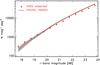 |
Fig. 1 Galaxy number counts per unit magnitude and per square degree. Red triangles are for VVDS measurements, with error bars representing the Poissonian uncertainty. The red line shows the median number counts of the 23 mock samples, and the grey area shows the 16th to 84th percentile range of the mock number counts distribution. The VVDS number counts agree well with the number counts obtained by McCracken et al. (2003) for the CFH12K-VIRMOS deep field. |
2.2.1. Mock sample number counts and mean inter-galaxy separation
Since we computed the galaxy 3D local environment in mock samples and compared it to that found in the VVDS, it is important to know possible similarities and/or discrepancies between the 3D galaxy distribution in the mock samples and that in the data.
In Paper I, we have shown that the light-cones used in our study give an average redshift distribution n(z) and galaxy clustering that are not in perfect agreement with the VVDS-02h measurements. In particular, we showed that the mock n(z) agrees with the observed n(z) in the range 0.5 < z < 1.8, but it overestimates the observed number of galaxies at z < 0.5, and underestimates it at z > 1.8. In addition, we have shown that the Munich semi-analytical model overestimates the VVDS clustering, and that this is mainly caused by an excess of the clustering signal for model red galaxies.
Figure 1 shows the number counts per square degree of VVDS-02h galaxies as a function of the observed IAB magnitude (that is, the VVDS selection magnitude). Number counts were computed from the parent photometric catalogue of ~40 000 sources, with stars removed using the method described in McCracken et al. (2003). The median number counts of the 23 mock samples used in this study are overplotted as a solid line. Figure 1 shows that the mock I-band number counts are higher than observational data at IAB > 22, but lower than the observed number counts at the brightest magnitudes (IAB < 20). Since faint galaxies are much more numerous than bright ones, mock samples contain on average ~10% more galaxies than observations2.
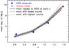 |
Fig. 2 Mean intergalaxy separation as a function of redshift in the four redshift bins used in C06 (0.25−0.6, 0.6−0.9, 0.9−1.2, 1.2−1.5). Red squares are the mean among the 23 Omocks used in this study, and the grey shaded area shows the 1 − σ scatter. Blue circles are for VVDS data. The thick solid line corresponds to the Omock with mean intergalaxy separation closest to the VVDS measurements at all redshift bins considered. The dashed line corresponds to the Omock with lowest number counts (in the total redshift range 0.25 − 1.5), and the dotted line to the Omock with highest number counts. |
Figure 2 shows the mean intergalaxy separation in the VVDS-02h field as a function of redshift. We overplot the same quantity computed in the Omocks. In the lowest redshift bin, all mock samples considered have a mean separation lower than measured in observed data. The average mean separation in Omocks is larger than the VVDS one in the range 0.6 < z < 1.2, and lower than the measured VVDS value for z > 1.2. At z > 0.6, there is at least one Omock with mean separation close to the VVDS one, but this is not the same Omock at all redshifts. In Fig. 2, we also show the mean intergalaxy separation for the Omock with the lowest number counts (dashed line). Its mean intergalaxy separation is larger or very similar to that of the VVDS (at least up to z = 1.2), as one would expect. The opposite is true for the Omock with the highest number counts (dotted line), up to z = 1.2. There is no Omock with number counts close to the observed ones at all redshift bins. The black solid line in the figure shows the Omock whose intergalaxy separation is on average closest to that of the VVDS at all redshift bins. Its counts are very close to the average among all the mock samples at each redshift (red squares). It does not correspond to the Omock with the lowest total number counts.
The results on the n(z), the number counts as a function of selection magnitude, and the mean intergalaxy separation are all related, showing that mock samples contain more galaxies than the VVDS-02h field.
2.2.2. The absolute magnitudes
In C06, red and blue galaxies have been defined using the rest-frame colour u∗ − g′. The u∗ and g′ (CFHT-LS filters) rest-frame magnitudes are not available on the Millennium database. Among the rest-frame absolute magnitude available for the De Lucia & Blaizot (2007), the closest to u∗ and g′ are those in the B and V Johnson filters. To be consistent with the analysis discussed in C06, we computed for our mock samples the u∗ and g′ absolute magnitudes using the same method as employed for the VVDS data (see below). We also computed the absolute magnitudes in the B and V Johnson filters for our mock samples, to compare them with the intrinsic ones available from the simulations. In this way, we can verify that the rest-frame magnitudes computation does not affect the intrinsic luminosity distribution.
For the VVDS data set, we computed the absolute magnitudes using the code ALF (Algorithm for Luminosity Function, Ilbert et al. 2005), based on a technique to fit the spectral energy distribution (SED). To reduce the dependency on templates, we derived the rest frame absolute magnitude in each band using the apparent magnitude from the closest observed band, shifted at the redshift of the given galaxy. In this way, we minimised the applied K-correction, which depends on the assumed template. The set of observed magnitudes used to derive the absolute magnitudes in C06 included BVRI bands from the CFHT-12K camera, and u∗, g′, r′, i′, z′-band data from the CFHT Legacy Survey. We have these observed magnitudes in our mock samples, and we used them to compute the intrinsic luminosities in the mock samples with the code ALF. We adopted the same cosmology as for the VVDS data, i.e. Ωm = 0.3, ΩΛ = 0.7, h = 0.7.
We compared the B and V absolute magnitudes (not including internal dust extinction) available on the Millennium database with the corresponding quantities computed with ALF. We found that the two sets of magnitudes are consistent within ~ 5%. The small difference between the two sets of magnitudes is slightly dependent on the galaxy luminosity, and does not depend on redshift within the redshift range explored. Because the B and V filters are very close to u∗ and g′, we are confident that the computation of u∗ and g′ rest-frame magnitudes using the method described above does not introduce any spurious effect either.
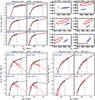 |
Fig. 3 Evolution of the luminosity function of galaxies in the mock samples compared to the results from the VVDS. Upper left panel: evolution of the luminosity function in the B-band for all galaxies in the Cmock 001b. Each panel refers to a different redshift bin, which is indicated in the label. The vertical dashed line represents the faint absolute limit considered in the STY estimate. The luminosity functions are estimated with different methods (see text for details) but for clarity we plot only the results from C + (symbols) and STY (lines). Red filled circles and lines are used for observational measurements while black empty squares and lines are used for the corresponding measurements from the Cmock. Upper right panel: 68% confidence ellipses for the α and M∗ parameters obtained using all galaxies in Cmock 001b (black ellipse), Cmock 022b (magenta ellipse), and Cmock 036d (cyan ellipse). The red thicker ellipse corresponds to the VVDS measurements; the red thick lines in the first and the last redshift bins show the uncertainties on one of the parameters obtained keeping the other fixed. Lower left panel: evolution of the luminosity function in the B-band for type 1 galaxies in the Cmock 001b. Lines and symbols have the same meaning as in the upper left panel. Lower right panel: evolution of the luminosity function in the B-band for type 4 galaxies in the Cmock 001b. Lines and of symbols have the same meaning as in the upper left panel. |
3. The B-band luminosity function
In this section, we compare the VVDS B-band (Johnson) luminosity function presented in Ilbert et al. (2005) and Zucca et al. (2006) with the corresponding quantity derived from the mock samples. In Zucca et al. (2006), we used only UBVRI3 apparent magnitudes as input for the SED fitting, because the CFHT-LS photometry was not available then. For consistency, we computed a second set of absolute magnitudes for the mock samples, using only these five observed bands. This second set of absolute magnitudes was used only for the LF presented in this section. For this analysis, we used the Cmocks and compared the model results with the observational estimate corrected for incompleteness.
The LF was computed using the code ALF (see Sect. 2.2.2), which implements several estimators: the non-parametric 1 / Vmax (Schmidt 1968), C + (Lynden-Bell 1971), SWML (Efstathiou et al. 1988), and the parametric STY (Sandage et al. 1979). We used the STY assuming a single Schechter function (Schechter 1976) parametrised in terms of a characteristic luminosity (L∗), a faint-end slope (α), and a normalisation (density) parameter (φ∗). For a more detailed description of the tool and the estimators, we refer the reader to Ilbert et al. (2005).
Ilbert et al. (2004) have shown that the LF measurement can be biased, mainly at the faint end, when the band used is far from the rest frame band in which galaxies are selected. This is due to the fact that, because of the K-correction, galaxies of different type are visible in different absolute magnitude ranges at a given redshift, even when applying the same flux limits. Moreover, in a flux-limited survey, this limit varies with redshift. When computing the VVDS LF, we avoided this bias by using in each redshift range only galaxies within the absolute magnitude range in which all SEDs are observable. We computed the LF in mock samples using the same method.
The upper left panel of Fig. 3 shows the luminosity function for one Cmock (cone 001b) in different redshift bins obtained with C + and STY methods. The luminosity functions derived with the other two methods (1 / Vmax and SWML) are consistent with those shown in the figure. The dashed red line and red filled circles in each panel show the corresponding results for the VVDS data. The vertical dashed line represents the faint absolute limit considered in the STY estimate.
The upper right panel of Fig. 3 shows the confidence ellipses of the α and M∗ parameters obtained in Cmock 001b (black ellipse), and also in Cmock 022b (magenta ellipse) and Cmock 036d (cyan ellipse), which are the mock samples with the lowest and highest number counts (see Sect. 2.2). The red thicker ellipse refers to the VVDS parameters, and the red thick lines in the first and last redshift bins show the uncertainties on one of the parameters derived by keeping the other one fixed. This figure shows that shape parameters α and M∗ measured for the three mock samples considered are consistent within the uncertainties. Some differences can be found in the normalisation parameters φ∗, reflecting the different number counts in the Cmocks.
Overall, there is a reasonable agreement between the LF in the VVDS and in the model, but with some significant discrepancies. In particular, we find that M∗ is almost always brighter and α almost always flatter in the VVDS than in the mock samples. In addition, there are significant differences in the normalisation of the model and data LFs, reflecting the differences in the number counts discussed in Sect. 2.2.1. In order to better explore these differences and to understand if they are induced by a specific class of objects, we derived the LF for galaxies of different types.
Zucca et al. (2006) split the global galaxy population into different spectro-photometric types. For each galaxy, they found the best template fitting the galaxy SED, choosing among four empirical templates from Coleman et al. (1980, CWW hereafter) and two starburst templates computed using GISSEL (Bruzual & Charlot 1993). They defined four galaxy types, corresponding to the four CWW templates (E/S0, early spiral, late spiral and irregular – type 1, 2, 3, and 4 respectively). Type 4 galaxies include the two starburst templates.
Here we apply the same classification scheme to galaxies in the mock samples, and derive their LFs as in Zucca et al. (2006). The lower panels of Fig. 3 show the LFs obtained for the two extreme galaxy populations (type 1 in the left bottom panel, and type 4 in the right bottom panel) in the Cmock 001b and in the VVDS data. Results from the Cmocks with highest and lowest number counts are similar. The figure shows a clear excess of type 1 galaxies in the mock samples at magnitudes fainter than the “knee” of the LF. In contrast, bright type 1 galaxies are under-represented in the model. For the latest-type galaxies (type 4), in Cmocks there is an excess of bright galaxies in the lowest redshift bins considered, and a slight deficit of fainter galaxies. Therefore, the steeper faint-end slope and the fainter M∗ found in the global LF in mock samples are caused by an excess of faint type 1 galaxies and deficit of bright type 1 galaxies, respectively. The effect on the global LF of the deficit of bright type 1 galaxies is less evident because it is compensated for by the excess of bright type 4 galaxies.
The excess of faint red galaxies in our model is a known problem that appears to be shared by most (all) semi-analytic models that have been published in recent years (see e.g. Wang et al. 2007; Fontanot et al. 2009; Weinmann et al. 2010, and references therein). This is also consistent with what we found in Paper I.
4. The colour–density relation
In C06, we analysed the colour − density relation as a function of both redshift and galaxy luminosity. Namely, we split our sample into four redshift bins (0.25 ≤ z < 0.6,0.6 ≤ z < 0.9,0.9 ≤ z < 1.2 and 1.2 ≤ z < 1.5), and in each redshift bin we studied the colour − density relation for galaxies with (MB − 5log h) ≤ − 19.0, − 19.5, − 20.0, − 20.5, − 21.0.
We stress that the density was computed using the entire available sample, irrespective of galaxy luminosity (see Sect. 4.1). Moreover, at , the VVDS sample does not contain enough galaxies with (MB − 5log h) ≤ − 20.5 because of the small probed volume. Therefore we excluded the two brightest luminosity thresholds from the analysis in this redshift range. We also know that VVDS samples brighter and brighter galaxies at higher redshift, because of its flux limit. Consequently we examined only galaxies with (MB − 5log h) ≤ − 19.5 and ≤ − 20.0 at and , respectively. These lower luminosity limits ensure that the considered subsamples are complete for all galaxy types.
4.1. The environment parameterisation
We refer the reader to C06 for a detailed description of the density computation method. Here we only give a brief summary.
For each galaxy at a comoving position r, C06 characterised its environment by means of the dimensionless 3D density contrast δ(r,R), smoothed with a Gaussian filter of dimension R: ![Mathematical equation: \hbox{$\del(\vec{r},R) = [\rho(\vec{r},R)-\overline{\rho}({\vec r})] / \overline{\rho}(\vec{r})$}](/articles/aa/full_html/2012/12/aa19554-12/aa19554-12-eq88.png) . When smoothing, galaxies are weighted to correct for various survey observational characteristics (sample selection function, target sampling rate, spectroscopic success rate, and angular sampling rate). Moreover, underestimates of δ due to the presence of edges were corrected by dividing the measured densities by the fraction of the volume of the filter contained within the survey borders.
. When smoothing, galaxies are weighted to correct for various survey observational characteristics (sample selection function, target sampling rate, spectroscopic success rate, and angular sampling rate). Moreover, underestimates of δ due to the presence of edges were corrected by dividing the measured densities by the fraction of the volume of the filter contained within the survey borders.
In C06, we calibrated the density reconstruction scheme using simulated mock samples extracted from GalICS (Hatton et al. 2003). The aim was to determine the redshift ranges and smoothing length scales R over which our environmental estimator reliably reproduced the underlying galaxy environment, as given by a 100% sampling rate catalogue with IAB ≤ 24. We concluded that we reliably reproduced the underlying galaxy environment on scales R ≥ 5 h-1 Mpc out to z = 1.5. In the present study, we did not use GalICS mock samples because they do not provide the information needed for our analysis (e.g. the observed magnitudes in all the VVDS bands). However, for a sanity check, we repeated the tests carried out in C06 with the mock samples used in the present study, and we confirmed our previous results on the reliability of the density reconstruction.
We computed the density field in both the Cmocks and Omocks, using the same method as in the VVDS data, and the same flux-limited (IAB ≤ 24) tracers population. As mentioned in Sect. 2.2, for the Omocks we adopted the same weighting scheme used for the VVDS data. In particular, we considered the target sampling rate, the spectroscopic success rate, and the angular sampling rate, and also accounted for survey boundaries. By construction, no correction is needed for the Cmocks since they have a 100% sampling rate. Moreover, to compute the density in the Cmocks, we started from the 1 × 1 deg2 mock samples from which they were extracted; accordingly, the density field depends very little (if at all) on the correction for boundary effects.
Figure 4 shows the density contrast distribution for Omocks and VVDS data for the different redshift bins and luminosity limits explored in C06. The average density distribution in Cmocks is very close to that in Omocks, but Cmocks have a smaller scatter around the mean. The density distribution in mock samples has longer tails towards high densities than VVDS, in particular at the lowest and highest redshift. Interestingly, these longer tails are not a consequence of the higher number counts in mock samples: the figure shows that the Omock with the lowest number counts also exhibits these tails at high density. Moreover, we verified that randomly depopulating the Omocks to have them match the observed number counts as a function of I-band and then re-computing δ does not suppress these tails. This means that in the Munich semi-analytical model, the 3D spatial distribution of galaxies is intrinsically different from that observed in the real Universe, and that the excess of the clustering signal in the mock samples is only in part caused by an excess of low- to intermediate-mass galaxies. In Paper I, we suggested that this might be due to the assumption of a WMAP1 cosmology in the Millennium Simulation, and in particular to the use of a high normalisation of the power spectrum (σ8). A lower value of σ8 would reduce the overall density contrast at any given redshift (Wang et al. 2008). Indeed, in Paper I we showed that if one converts the correlation functions in the model to those expected assuming a lower value of σ8, the signal decreases at all scales. However, in Paper I we did not change other cosmological parameters. Recently, Guo et al. (2012) rescaled the Millennium Simulation to the WMAP7 (Komatsu et al. 2011) cosmological parameter values. These authors showed that the effects of the decreased σ8 are compensated for by the higher value of Ωm. Therefore, the assumption of a WMAP1 cosmology cannot explain the excess of clustering in our mock samples.
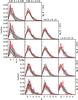 |
Fig. 4 Density contrast distribution in the different redshift bins and luminosity limits. Red thick solid line: VVDS sample; black dotted line: Omock with lowest number counts; black thin solid line: average of the Omocks; grey area: 1-σ scatter of Omocks. |
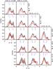 |
Fig. 5 Colour distribution in the different redshift bins and luminosity limits. Red thick solid line: VVDS sample; black thin solid line: average of the Omocks; grey area: 1-σ scatter of Omocks. Red short arrows represent the fixed colour cuts used to define red ((u∗ − g′) ≥ 1.1) and blue ((u∗ − g′) ≤ 0.55) galaxies in C06. Blue long arrows indicate which colour cuts should be used in the mock samples to achieve the same percentage of red and blue galaxies (irrespectively of environment) as in the VVDS for each redshift bin and luminosity limit. |
4.2. The colour distribution
Cucciati et al. (2006) empirically defined red and blue galaxies to be the two extremes of the u∗ − g′ colour distribution. Namely, red galaxies are defined as those with u∗ − g′ ≥ 1.1 and blue as those with u∗ − g′ ≤ 0.55. These colour cuts roughly correspond to the two peaks of the bimodal colour distribution in the VVDS. These authors kept these limits fixed for all luminosities and redshift bins.
From Paper I and Sect. 3, we know that the colour distribution in the model is different from the observed one. Figure 5 shows the colour distributions in Omocks and VVDS for the different redshift bins and luminosity limits. The 1-σ scatter for the Cmocks is narrower than that of the Omocks, but the average values of the two kinds of mock samples are very close. We note that at intermediate redshifts (0.6 < z < 1.2), the blue cloud is more populated in the model than in the VVDS, especially for bright galaxies (MB ≤ − 20). At these redshifts and luminosities, the blue peak of the bimodal colour distribution in the mock samples is between 30% to 100% higher than that of the VVDS, while having roughly the same width. Still, if we consider only the tail of the bluest galaxies (u∗ − g′ ≤ 0.55, as defined in C06), there are fewer of them in the model than in the VVDS, especially for faint galaxies. In contrast, the peak of the red galaxy population is higher in the model than in the data for fainter galaxies, and it corresponds to redder colours. These results agree with those presented in Paper I and with the discrepancies discussed in Sect. 3.
Therefore the mix of galaxy populations (and colours) is different in the model and in the VVDS. As a consequence, if we use the same colour cuts in the mock samples as in the VVDS, we obtain different fractions of red and blue galaxies (independently of the environment). Figure 6 shows the fraction of red and blue galaxies as defined in C06 in the VVDS as a function of redshift and for the different luminosity limits. The corresponding fractions in the mock samples are different from those in the VVDS sample. The colour dependency on luminosity is also less evident in the model than in the VVDS.
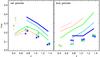 |
Fig. 6 Fraction of red ((u∗ − g′) ≥ 1.1, left panel) and blue ((u∗ − g′) ≤ 0.55, right panel) galaxies as a function of redshift for different luminosity thresholds. Lines are for VVDS data, triangles for Omocks, and squares for Cmocks. The colour/thickness code is the following: from magenta/thin to blue/thick we consider galaxies with (MB − 5log h) ≤ −19.0, −19.5, −20.0, −20.5, −21.0. Each triangle(/square) represents the mean value of all Omocks(/Cmocks). |
Figure 6 also shows that the fraction of red galaxies is slightly lower in Omocks than in Cmocks at all redshifts, especially at z < 0.6, where it is lower by 5 − 8% depending on the luminosity cut. It is known that the VVDS observational strategy misses a very small fraction (~4%) of very red galaxies in particular at low z (see e.g. Franzetti et al. 2007). This bias is mainly due to the optimisation for slit positioning, which preferentially targets smaller galaxies in I-band. At low redshift, brighter and bigger galaxies in the observed I-band are the early types. We will show that this small loss of red galaxies at z < 0.6 does not alter the colour − density relation in Omocks, and we believe that this applies to the observed data as well. We also verified that the global sampling rate does not vary as a function of the density computed on a 5 h-1 Mpc scale in the Omocks for the different redshift bins and luminosity cuts.
Figure 5 also shows the two colour cuts of C06 (red arrows) and the colour cuts we would need to use in the mock samples to obtain the same fractions of red and blue galaxies as in the VVDS for each redshift bin and luminosity cut (blue arrows). For this plot we considered all galaxies, independently of their environment. To compute the colour − density relation in mock samples, we took the colour cuts corresponding to the same fraction of red and blue galaxies as in the VVDS, as this choice follows the same rationale used in C06, i.e. considering the extremes of the colour distribution. This makes the comparison with VVDS more straightforward and provides the same overall normalisation in the colour − density relation as in the VVDS. As a test, we also computed the colour − density relation in the mock samples using colour cuts that correspond roughly to the two peaks of the mock colour distribution. As for the VVDS, we kept these cuts constant at all redshifts and for all luminosities. The colour − density relations obtained in this way are very similar to those obtained using variable cuts that reproduce the observed fraction of red and blue galaxies. So our results are robust against this choice.
4.3. The colour − density relation up to z ~ 1.5
We reproduced the analysis on the colour − density relation as in C06, using both Cmocks and Omocks samples.
Figure 7 shows the fraction of red (fred) and blue (fblue) galaxies as a function of the density contrast δ for different redshift bins and for different luminosity thresholds. Red and blue symbols are for Omocks, while green and orange shaded areas show the error contours for the VVDS. Figure 8 shows the corresponding quantities for Cmocks. The results from Omocks have larger error bars because of the larger Poisson error, but the average is very close to that of Cmocks. In each mock sample, we computed fred and fblue as a function of δ in three equipopulated density bins (choosing the median δ value as representative for the bin). The points in Figs. 7 and 8 are the average of the mock samples on both the x- and y-axis. Vertical error bars are the sum in quadrature of the rms around the mean of the 23 mock samples and the typical error (Poisson) of one single cone. In this way, we simultaneously account for cosmic variance among different realizations and for the typical Poisson noise in a single realization.
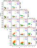 |
Fig. 7 Colour − density relation in Omocks: blue squares represent the fraction of blue galaxies (fblue) and red triangles the fraction of red ones (fred). x- and y-axis positions are mean values of the x- and y-axis values for the 23 mock samples. Vertical error bars include the scatter among the 23 cones and the typical (mean) error in each cone on the computation of fblue or fred. Orange and green contours represent fred and fblue in the VVDS sample (from C06). The numbers quoted in each panel are the total number of red and blue galaxies in the VVDS data and in the mock samples (average on the 23 cones), with the same colour-code as for the symbols. For VVDS observed data we define red galaxies as those with (u∗ − g′) ≥ 1.1 and blue galaxies as those with (u∗ − g′) ≤ 0.55 at all z and for all luminosities. In the mock samples, the definition of red and blue galaxies varies with z and luminosity so that there is the same fraction of red and blue galaxies as in the VVDS (irrespectively of environment) in each redshift bin and for each luminosity limit (see the blue arrows in Fig. 5). |
4.3.1. The effects of a < 100% sampling rate on the colour − density relation
We find that the average colour − density relation in Omocks is very similar to that found in Cmocks. This means that, on average, the VVDS observational strategy does not significantly alter the observed environmental trends for galaxy colours on a ~5 h-1 Mpc scale. This does not exclude the possibility that there may exist at least one mock in which the colour − density relation is strongly affected by the VVDS observational strategy. In order to address this question, we performed a linear fit of fred as a function of δ in each luminosity and redshift bin considered, and compared the slope of this linear fit in Cmocks and Omocks. We performed the same calculation for fblue.
In Fig. 9, we show the slopes obtained for each cone in the four redshift bins and for galaxies with MB ≤ − 20 (i.e., the third row of Fig. 7). We plot the slope values for both Cmocks and Omocks. The x-axis value is arbitrary, but for each pair of Cmocks and Omocks extracted from the same light cone we used the same x-axis value for fred and fblue. Figure 9 shows that a positive slope in Cmocks never becomes negative in the Omocks, or vice- versa, except for a few exceptions at 0.25 < z < 0.6 that may be due to low number statistics. The figure also shows the average slopes for Cmocks and Omocks together with the slopes from the VVDS sample.
This figure shows that going from Cmocks to Omocks, the colour − density relation becomes slightly shallower, but does not disappear or reverse. This suggests that the trends found in C06 (the flattening and possibly the reversal of the colour − density relation going to high redshift) are not caused by biases in the VVDS observational strategy (uneven and < 100% sampling rate, field shape, etc.).
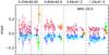 |
Fig. 9 Slopes of the colour − density relation linear fits for the 23 Cmocks and the 23 Omocks for galaxies with MB ≤ −20 in the four redshift bins (label on the top), as in the third row of Figs. 7 and 8. Red and blue small diamonds: red and blue galaxies in each Omock; light purple and cyan small diamonds: red and blue galaxies in each Cmock. Red and blue big triangles: mean values of red and blue small diamonds, with the vertical error bar being the rms among all 23 mock samples. Light purple and cyan big squares: mean values of light purple and cyan small diamonds, with their rms. Orange and green circles: slope and its error for VVDS observed data (from C06) for red and blue galaxies, respectively. |
4.3.2. Observed data versus mock samples
In the previous section, we showed that the VVDS strategy does not significantly alter the colour − density relation potentially observable in a survey with 100% sampling rate. Now we analyse the colour − density relation in the VVDS observed sample and the one found in mock samples, with the aim to contrast galaxy evolution in simulations and in the real Universe.
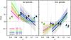 |
Fig. 10 Slopes of the linear fits of the colour − density relation in each panel of Figs. 7 and 8, for fred on the left panel and fblue in the right panel. Lines and shaded areas: VVDS observed data with error. Triangles: Omocks. Squares: Cmocks. Different colours of lines and symbols are for the different luminosity thresholds, as indicated in the labels. In each redshift bin, delimited by vertical dashed lines, all points should be considered at the same (central) x-value, but they are shifted for clarity. |
Some interesting trends are visible in Figs. 7 and 8. First, the density contrast in mock samples spans a wider range than observed data, extending towards higher densities. This mirrors the stronger clustering found in the model that we discussed in Paper I and in Sect. 2.2. Second, error bars for Cmocks are smaller than those of VVDS, although they include the cosmic variance among the 23 cones. This is because the Poisson noise is much lower, as can be seen by comparing the number of galaxies shown in the labels of Fig. 8. In contrast, error bars for Omocks are larger than those of VVDS, because their Poisson noise is similar but they include cosmic variance as well. These trends are similar for all redshift bins and luminosity thresholds.
At a fixed luminosity threshold, the colour − density relation in VVDS is steeper than in the model at 0.25 < z < 0.6, very similar to that in the model at 0.6 < z < 0.9, and shallower than in the model at z > 0.9. In particular, the colour − density relation in the VVDS data is almost flat at 0.9 < z < 1.2, and it seems to be inverted at z > 1.2 (i.e., at these high z blue galaxies reside preferentially in high-density regions). In contrast, the mock colour − density relation varies only weakly as a function of redshift with no significant flattening, and definitely no inversion at higher redshift. We analysed the colour − density relation in detail in the pair of Cmock/Omock with the lowest number counts. As for the density distribution shown in Fig. 4, this cone shows a colour − density relation very close to the average of the 23 mock samples. We will discuss the implications of these general trends in Sect. 6.
Figure 10 shows the slopes obtained from fitting the colour − density relation in the mock samples and compares them with those obtained from the VVDS data. Although the error bars for the VVDS data are large, the evolution of the colour − density relation with redshift is clear. In contrast, no evolution is found in Omocks or in Cmocks. Moreover, while in the VVDS data there is a trend for steeper colour − density relation for brighter galaxies, this trend is much less clear (if at all there) in mock samples. We note that the dependence of the colour − density relation on galaxy luminosity is a controversial issue in the literature. It has been found in C06, but not in Cooper et al. (2007), who studied the colour − density relation in the DEEP2 survey (Davis et al. 2003), selected with a slightly brighter flux limit than the VVDS. In Cucciati et al. (2010), we did not find any luminosity dependency in the zCOSMOS Bright survey (Lilly et al. 2009), which is much brighter (IAB ≤ 22.5) than the sample used in C06.
The comparison between the slopes measured in the mock samples and those measured from data may suffer from the fact that the density distribution in the model extends to higher densities than observed. Because of this, in almost each panel of Figs. 7 and 8 the point at highest density has a higher x-value in mock samples than in the VVDS, even if fred or fblue are very similar. Thus the slope may be flatter in mock samples than in the VVDS, only because of the different density distribution. To perform a fairer comparison, we computed the fractional increment of fred and fblue from the lowest to the highest density bin in each panel of Figs. 7 and 8. The results for both the observations and the model are very similar to those of Fig. 10, and confirm that there is no significant flattening of the colour − density relation in the mock samples.
The results discussed above confirm that, at least in the semi-analytical model used in our study, the environment shapes galaxy evolution (as a function of z) in a different way than we observe in the real Universe.
5. Why is there a colour − density relation?
Different methods to parameterise the local density around galaxies have been used in the literature for different galaxy samples. Often it is the survey strategy itself that dictates the optimal (less biased) environment parameterisation for each specific data set. It is not yet clear what the “physical meaning” of these parameterisations is, e.g. how the density field compares to the underlying dark matter distribution, and in particular, how the estimated “density” relates to the mass of the DM halos in which the galaxies reside.
Some recent studies (Haas et al. 2012; Muldrew et al. 2012) have focused on a comparison between different environmental definitions and the information on the parent DM halo mass. These studies have considered results at z ~ 0, and have not entered the details of different observational strategies and/or selections. Given the evolution of the mean density and of the mass growth of structures, it would be very interesting to extend this detailed analysis to higher redshift. It should be noted, however, that results might well depend on the details of each particular survey and, as such, they are difficult to generalise.
We have taken advantage of the available MILLENNIUM mock samples to understand the origin of the colour − density relation as observed in VVDS data. To do this, we explored the relationship existing between the estimated density contrast and the mass of the DM haloes in which galaxies reside. For each galaxy in our mock samples, we retrieved its parent DM halo using the public database built for the Millennium Simulation (Lemson & Virgo Consortium 2006). Here, a “DM halo” corresponds to a halo identified in the Millennium Simulation using a friends-of-friends algorithm (“FOF halo” from now on), with a linking length of 0.2 in units of the mean interparticle separation. Our results are shown in Fig. 11 for galaxies with MB ≤ − 20. We repeated our analysis for both Cmocks and Omocks (top and bottom panels of the figure) to test the influence of the VVDS observational strategy. In each panel, we distinguish central galaxies from satellite galaxies. On the right vertical axes of Fig. 11, we indicate the typical radius (in h-1 Mpc) of haloes with mass given by the corresponding value on the left axis4. This shows that the scale on which δ is computed is much larger than the size of the structures in which galaxies reside.
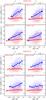 |
Fig. 11 Total halo mass as a function of the local density contrast computed in this work in different redshift bins (as in the labels) for galaxies with MB ≤ − 20. The values of the density contrast are indicated as log (1 + δ) in the bottom x-axis and as δ in the top x-axis. The halo is the FOF halo in which the galaxy reside (the halo of the group/cluster of which the galaxy is member). Four top panels: Cmocks. Four bottom panels: Omocks. Red circles and contours refer to central galaxies, blue squares and contours to satellite galaxies. Each panel includes all the 23 mock samples. Lines represent the isodensity contours of all the galaxies in the panel. For clarity, single galaxies are plotted as small dots only outside the lowest density contour. Filled red circles (/blue squares) are the median values in density bins for central (/satellite) galaxies. The error bars represent the 16% and 84% of the halo mass distribution in each density bin. On the right vertical axis of each panel, we show the typical virial radius (in h-1 Mpc) corresponding to the halo mass on the left vertical axis. |
Figure 11 shows a very general trend: galaxies belonging to massive halos (mass ≳ 1013 M⊙ / h) reside only in over-dense regions on a 5 h-1 Mpc scale, even if the virial radius of these halos is much smaller than the filtering scale. This happens because the density in these regions is boosted to high values by the large number of galaxies residing in these massive haloes, and is not affected significantly by the large-scale structure around them. In contrast, lower mass halos span the entire density range, because their density within the virial radius is not very high, so the density on larger scales depends also on the surrounding structures.
From Fig. 11, it is clear why we should expect a colour − density relation on a 5 h-1 Mpc scale. There is an increase of the parent halo mass with increasing δ for satellite galaxies, although with a large scatter. This relation is driven by the large number of satellites in the most massive halos. The figure shows that, if a satellite has a high measured δ on the scale considered, it more probably belongs to a massive cluster than to a low-mass halo. If we assume that clusters have a higher fraction of red satellites than groups (see e.g. De Lucia et al. 2012), we expect a colour − density relation for satellite galaxies.
For central galaxies, the correlation between halo mass and δ on 5 h-1 Mpc is weak, but there is still a trend for central galaxies in highest density regions to be scattered to higher mass haloes. This happens because the most massive haloes tend to be clustered. Then, if we assume that central galaxies in more massive haloes are redder than central galaxies of lower mass haloes, we would expect to have a higher fraction of red galaxies in higher density regions.
In Figs. 7 and 8, we showed that we do find a colour − density relation for model galaxies. We verified that this relation is maintained when considering only centrals or only satellites galaxies. The colour − density relations for the two populations are similar and agree with the global colour − density relation.
As redshift increases, the VVDS flux limits select increasingly brighter galaxies. Thus, the fraction of observed satellites (that dominate the intermediate to faint end of the LF) decreases, so that the correlation between density and halo mass becomes less significant for satellites as well. This is also evident by comparing Cmocks with Omocks: the VVDS observational strategy applied in Omocks reduces the fraction of observed satellites in massive clusters, flattening the relation between halo mass and δ. This happens because the size of the slits in the spectrograph prevents us from targeting in one single pass galaxies with small projected distances. The VVDS multi-pass strategy alleviates this problem but small-scale very dense regions (such as the central regions of galaxy clusters) are still undersampled with respect to regions that are less crowded. At the highest redshift considered, where the effect of the low sampling rate is added to the effect of the flux limit, we do not see any clear correlation, even for satellite galaxies.
In a survey like the VVDS, given its flux limit, the fraction of satellites galaxies (fsat) is low, and it decreases with z. In particular, for galaxies with MB ≤ − 20, it varies from ~ 15% to ~ 8% going from the lowest to the highest redshift. Consequently, we expect that central galaxies have an important role in shaping the observed colour − density relation. We return to this in Sect. 6.
6. Discussion
As shown in previous studies and above, the Munich semi-analytical model does not reproduce some of the galaxy properties measured from the VVDS. In particular, there is an excess of sources for IAB < 24 in the model, mainly due to an excess of faint red galaxies. The model also exhibits a slight excess of bright blue galaxies, and the galaxy clustering is overpredicted. We have studied how the 3D galaxy distribution in this model affects galaxy colours up to z = 1.5. The aim of our analysis is to understand how environment affects galaxy evolution by modulating internal physical processes, and to what extent this is reproduced by the model used in this study.
Our analysis demonstrates that the colour − density relation, computed on a 5 h-1 Mpc scale, does not evolve significantly with redshift in the Munich semi-analytical model, at least from z = 0.25 to z = 1.5. This relation does not evolve even if we consider centrals and satellites separately. In contrast, significant evolution has been observed in different samples and on different scales (e.g. C06; Cooper et al. 2007; Cucciati et al. 2010), and C06 even observed a possible inversion in such relation at z ≳ 1.2.
Given the striking difference between observational results and model predictions about the evolution of the colour − density relation, some questions arise: within a cosmological framework, do we expect an epoch when the colour − density relation is inverted? On which scale should such an inversion be measured? And are the physical processes responsible for such a relation included in the model that we have considered in this study?
Qualitatively, we expect a reversal of the colour − density relation at an early epoch and on the scale of galaxy groups due to starburst events in gas-rich mergers. In this scenario, two young and gas-rich galaxies will evolve differently if one remains in isolation (passive evolution) and the other merges with another gas-rich galaxy (this will trigger a starburst episode whose intensity depends on the mass ratio and on the amount of gas available). During the merger, and for some time after it has been completed, the fraction of bright star-forming galaxies should be higher in high densities than in low densities. This simple scenario is complicated by the fact that lower density environments will also contain young star-forming galaxies, although these might be fainter than the VVDS flux limit. Another complication is caused by dust attenuation: a large part of the galaxies that are classified as red might be forming stars at some significant rate, and this fraction might evolve as a function of cosmic epoch and/or luminosity and environment. For example, De Lucia et al. (2012) found that the fraction of red star-forming galaxies decreases with increasing mass and with decreasing distance from the cluster centre. Moreover, it has been observed that dust attenuation clearly evolves with redshift (see e.g. Cucciati et al. 2012).
A similar scenario, based on starburst events in wet mergers, has been proposed by Elbaz et al. (2007), who found an inversion of the star formation-density relation comparing the GOODS fields at high redshift with SDSS data. In particular, they found the mean star formation rate to be higher in high densities at z ~ 1, on a 1.5 h-1 Mpc scales. Their galaxy selection is similar to that adopted in C06 at the same redshift (MB ≤ −20). In their sample, these galaxies are often located in correspondence to local density enhancement on the scale of clusters/groups (~1 h-1 Mpc). Elbaz et al. (2007) also measured the SF-density relation in SAMs (the model by Croton et al. 2006 applied on the Millennium Run by Kitzbichler & White 2007), applying the same methods as in their observational sample, and they did not find any reversal at z ~ 1, but a mild reversal of the SF-density relation at z ~ 2. Wang et al. (2007) carried out a similar analysis focusing on the relation between the average D4000 Å break and the local density computed on a ~2 h-1 Mpc scale. In agreement with what was discussed above, they found that in the Munich semi-analytical model there is no significant weakening of the D4000 Å-density relation up to redshift ~3.
It is interesting that in C06 we found a possible reversal of the colour − density relation on ~5 h-1 Mpc scales, which is much larger than those of galaxy groups. A few previous studies have argued that large scale environmental trends are the residual of the trends observed on much smaller scales (Kauffmann et al. 2004; Blanton et al. 2006; Cucciati et al. 2010; and see also Wilman et al. 2010). We cannot establish if this is also the case in C06, as the scale used to compute the density contrast was the smallest allowed by the VVDS sampling rate to guarantee a reliable reconstruction of the density field (see the tests in C06). In addition, the ~5 h-1 Mpc scale should be compared to the typical scales of processes happening “around” clusters, such as for instance the infall of galaxies and groups onto larger structures. One may also expect that this scale varies with redshift because structures grow with time.
It is interesting that in the Munich semi-analytical model we find the same (not-evolving) colour − density relation for satellites and central galaxies separately (see Sect. 5). We should consider that some physical processes that might be at play in determining the evolution and the inversion of the colour − density relation are modelled in a fairly crude way. For example, starbursts triggered by mergers are “instantaneous” (i.e. their time-scale corresponds to the integration time-scale adopted in the model), and the model does not account for star formation episodes that might be triggered during fly-by. In addition, in this model (like in most of the recently published ones) there is a significant excess of red (passive) galaxies with respect to observations. In particular, the model galaxies in the region of infall around clusters are redder than in the real Universe, because most of the galaxies in a group that is infalling in a cluster will be already too red in the model.
Since the model does not match the expected evolution of the colour − density relation as a function of redshift, we can modify the colour distribution in the model by making simple assumptions, and see how the colour − density relation changes. For example, we verified what happens if we assume that the colour of central galaxies is correctly reproduced by the model, and that satellites are either all red or all blue. The results of this test are shown in the top panel of Fig. 12. Since fsat increases with density, at all z, if satellites are all red, the increase of fred as a function of density would be even steeper than what is found in the model. This would increase the disagreement between data and models. If we assume that satellites are all blue, which is unrealistic, we find that the fred-δ relation flattens at all redshifts, with the flattening being slightly more significant at low redshift. This is because fsat decreases with increasing redshift (see Fig. 11). This is, however, not enough to have a flat relation at z > 1.2, as observed for VVDS. In addition, assuming all satellites are blue would yield an almost flat fblue-δ relation at z > 1.2 but would invert the relation at z < 0.9, in contrast to what is observed.
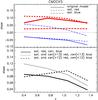 |
Fig. 12 Top panel. Slope of the linear fit of the fred-density relation (thick red lines) and of the fblue-density relation (thin blue lines) as a function of redshift in Cmocks. Only galaxies with MB ≤ −20 are considered. Solid line: slopes as found in the model, the same as in Fig. 10. Dashed and dot-dashed lines: slopes for two different assumptions about the colour distributions of satellite galaxies. We assume that centrals galaxies have the same colour as in the model, but now we assume that satellites are either all red (dashed line) or all blue (dot-dashed line). Bottom panel. Slope of the linear fit of the fred-density relation as a function of redshift in Cmocks, for three different assumptions about the colour distributions of central and satellite galaxies. Solid line: all satellites are red, and all centrals are blue. Dotted line: all satellites and centrals residing in DM halos with virial mass ≥ 1013 M⊙ / h are red, while all other centrals are blue. Dashed line: like the dotted line, but in this case the red centrals are those residing in DM halos with virial mass ≥ 1012 M⊙ / h. For this plot we use the 23 Cmocks together, and we keep fsat increasing with δ and decreasing with z as we find in the mock samples. |
This suggests that an inaccurate modelling of the physics of satellite galaxies cannot be solely responsible for the disagreement we find between models and data, and that this discrepancy also signals the need for a revised treatment of central galaxies.
In order to gain insight on this, we assumed that the model predicts the correct increase (decrease) of fsat as a function of density (redshift), and that all satellites are red while all central galaxies are blue. Since fsat decreases with increasing redshift, this would flatten the fred-δ relation with increasing redshift, as shown in the bottom panel of Fig. 12. The figure shows that a flattening would be observed also if we assumed that all satellites and central galaxies of haloes more massive than 1013 M⊙ / h (dotted line) are red, and that all other central galaxies are blue. In contrast, if we assume all satellites and all central galaxies of haloes more massive than 1012 M⊙ / h (dashed line) to be red, the evolution of the slope of the fred-δ is not monotonic.
This toy-model is simplistic, because we considered all satellites to be red, for instance, and we did not include any redshift evolution of the colour-mass relation for central galaxies. However, this simple exercise tells us that for a survey like the VVDS, the role of central galaxies in the evolution of the colour − density relation is very important, and that the modelling of these galaxies needs to be revised in our model as well.
Additional work is therefore needed to understand the physical processes that drive the flattening (and possibly inversion) of the colour − density relation in real observations, and how they can be properly included in the context of hierarchical galaxy formation models. An interesting approach would be to use the accretion histories of model galaxies in different density bins, as in De Lucia et al. (2012). If galaxies in low- and high-density regions have spent different fractions of their life-time in high-density environments, we expect them to have different colours. Using this approach, it will be possible to compare, and possibly to link, the formation histories of galaxies at low- and high-redshift, and to shed light on the evolution of the colour − density relation. We will address this issue in future work.
7. Summary and conclusions
We used galaxy mock samples constructed from a semi-analytic model coupled to a large cosmological simulation to compare the observed colour − density analysis up to z ~ 1.5 presented in Cucciati et al. (2006) with model predictions, carefully reproducing the observational selection and strategy adopted for the VVDS Deep sample.
To be specific, we used 23 galaxy mock samples with the same flux limits as adopted in the VVDS-Deep survey (Cmocks). These were extracted from the Millennium Simulation, applying the semi-analytical model by De Lucia & Blaizot (2007). From each of these mock samples, a subsample of galaxies was extracted (Omocks) that mimick the VVDS survey observational strategy (sampling rate, slit positioning, etc.). We then computed the galaxy luminosity function and the colour − density relation in the mock samples, with the same methods as employed for the VVDS survey. Our results can be briefly summarised as follows:
-
1)
The mock samples based on the Munich semi-analytical model contain on average ~10% more galaxies than the VVDS sample. This is consistent with results obtained in Paper I.
-
2)
The rest-frame B-band LF in mock samples agrees roughly with that derived from the observations, but it has a slightly steeper slope, especially at 0.2 < z < 0.8. This is expected, given the excess of galaxies in the model in this redshift range. We also computed the LF for early- and late-type galaxies separately, and showed that the model overpredicts the number densities of faint early-type galaxies and that of bright late-type galaxies.
-
3)
The density distribution computed with the same method as in the VVDS has more prominent tails towards higher densities in the mock samples at any redshift and luminosity explored. This is not caused by the larger number counts in the model, but is related to an intrinsically different galaxy distribution, which also reflects in a stronger clustering signal in mock samples (see Paper I).
-
4)
The colour − density relation in Omocks agrees very well with that in Cmocks (it is only more noisy and slightly less significant in Omocks). This enhances the confidence that the evolutionary trend of the colour − density relation in the VVDS-Deep survey is not caused by any severe bias introduced by the survey observational strategy.
-
5)
The colour − density relation in the model does not evolve significantly from z = 0.25 to z = 1.5, in contrast with a significant evolution measured in the data. In particular, we find no flattening (or inversion) of the colour − density relation at higher redshift, at least up to the redshift explored by the VVDS data and on the same scale.
-
6)
Given the relation between the measured density contrast and the virial mass of the halos where galaxies reside, we do expect and find a colour − density relation both for central and satellites galaxies. Both are very similar to the relation found for the global population. We argue that the lack of evolution in the colour − density relation in mock samples cannot be due only to inaccurate prescriptions for the evolution of satellites galaxies, and that the treatment of the central galaxies has to be revised as well.
A reversal of the colour − density relation is expected in a scenario in which wet mergers of young galaxies trigger an enhancement of star formation in the interacting galaxies. In this scenario, a reversal of the colour − density relation should be observed on the scale of galaxy groups. A reversal of the star formation-density relation has been observed on such scales at z ~ 1 (Elbaz et al. 2007). However, it is not straightforward to correlate galaxy SF with colours because of dust reddening. Therefore it is unclear that what we measure on a 5 h-1 Mpc scale is a mirror of what is happening on smaller scales. The lack of evolution of the colour − density relation in the model, on a 5 h-1 Mpc and at least up to z = 1.5, suggests that the evolution has happened at z > 1.5, and/or that the model galaxy colour is affected by environment on scales much smaller than 5 h-1 Mpc, with no corresponding trends on larger scales.
The disagreement between the evolution of the colour − density relation in the model and in observed data deserves a more detailed investigation as it can clarify what are the physical processes that drive the observed flattening (and inversion), and to what extent these physical processes are included in recent models of galaxy formation. It would be also important to view the role of central and satellites galaxies separately. We focused on mock samples that reproduce the VVDS observational strategy. With these mock samples it is not possible to proceed in this analysis, because the flux limits prevent us from collecting enough galaxies to study the small-scale environment in detail at the highest redshift, even if we had a 100% sampling rate. With mock samples it is possible to go beyond the luminosity and redshift range explored by the VVDS, but currently there would be no suitable counterpart among the available data sets. For example, Knobel et al. (2012) successfully separated central and satellites galaxies in the zCOSMOS group catalogue, but this catalogue reaches only z = 1, and the flux limit (IAB ≤ 22.5) is brighter than that in the VVDS. Gerke et al. (2012) used data from the DEEP2 survey to compute a group catalogue that extends at z > 1, but they did not distinguish between central and satellite galaxies. Moreover, the DEEP2 flux limit is very similar to that of the VVDS, so at z > 1 the study of satellite galaxies would be difficult. Therefore, deeper spectroscopic surveys with a higher sampling rate are needed to shed light on the physical processes that establish the observed relation between colour and density.
Figure 3 of Paper I shows that I-band counts in the mock samples agree very well with those from the VVDS. The discrepancy with the results presented here is caused by an error in the plotting routine used for that figure. This does not alter the conclusions of that section of Paper I, however, which are based on the i′-band counts (Fig. 4 in Paper I): the i′-band counts in the mock samples are higher than in the VVDS, consistent with our I-band results.
U-band from the MPI telescope, and BVRI from the CFHT-12K camera as described in Sect. 2.1
The virial mass is computed using the simulated particles, as the mass enclosed within a sphere that corresponds to an overdensity of 200 times the critical density. The virial radius is computed from the virial mass, through scaling laws based on simulation results and the virial theorem.
Acknowledgments
We would like to thank the referee for helpful suggestions that improved the paper. The Millennium Simulation databases used in this paper and the web application providing online access to them were constructed as part of the activities of the German Astrophysical Virtual Observatory. We are grateful to Gerard Lemson for setting up an internal data base that greatly facilitated the exchange of data and information needed to carry out this project, and for his continuous help with the database. O.C. thanks the INAF-Fellowship program for support. G.D.L. acknowledges financial support from the European Research Council under the European Community’s Seventh Framework Programme (FP7/2007-2013)/ERC grant agreement No. 202781. Part of this work was supported by PRIN INAF 2010 “From the dawn of galaxy formation to the peak of the mass assembly”. The results presented in C06 have been obtained within the framework of the VVDS consortium, and we thank the entire VVDS team for its work.
References
- Abbas, U., & Sheth, R. K. 2005, MNRAS, 364, 1327 [NASA ADS] [CrossRef] [Google Scholar]
- Bielby, R., Hudelot, P., McCracken, H. J., et al. 2012, A&A, 545, A23 [NASA ADS] [CrossRef] [EDP Sciences] [Google Scholar]
- Blaizot, J., Wadadekar, Y., Guiderdoni, B., et al. 2005, MNRAS, 360, 159 [NASA ADS] [CrossRef] [Google Scholar]
- Blanton, M. R., Eisenstein, D., Hogg, D. W., & Zehavi, I. 2006, ApJ, 645, 977 [NASA ADS] [CrossRef] [Google Scholar]
- Bruzual, A. G., & Charlot, S. 1993, ApJ, 405, 538 [NASA ADS] [CrossRef] [Google Scholar]
- Bruzual, G., & Charlot, S. 2003, MNRAS, 344, 1000 [NASA ADS] [CrossRef] [Google Scholar]
- Chabrier, G. 2003, PASP, 115, 763 [NASA ADS] [CrossRef] [Google Scholar]
- Coleman, G. D., Wu, C., & Weedman, D. W. 1980, ApJS, 43, 393 [NASA ADS] [CrossRef] [Google Scholar]
- Cooper, M. C., Newman, J. A., Coil, A. L., et al. 2007, MNRAS, 376, 1445 [NASA ADS] [CrossRef] [Google Scholar]
- Cowie, L. L., Songaila, A., Hu, E. M., & Cohen, J. G. 1996, AJ, 112, 839 [Google Scholar]
- Croton, D. J., Springel, V., White, S. D. M., et al. 2006, MNRAS, 365, 11 [NASA ADS] [CrossRef] [Google Scholar]
- Cucciati, O., Iovino, A., Marinoni, C., et al. 2006, A&A, 458, 39 [NASA ADS] [CrossRef] [EDP Sciences] [Google Scholar]
- Cucciati, O., Iovino, A., Kovač, K., et al. 2010, A&A, 524, A2 [NASA ADS] [CrossRef] [EDP Sciences] [Google Scholar]
- Cucciati, O., Tresse, L., Ilbert, O., et al. 2012, A&A, 539, A31 [NASA ADS] [CrossRef] [EDP Sciences] [Google Scholar]
- Davis, M., Faber, S. M., Newman, J., et al. 2003, in Discoveries and Research Prospects from 6- to 10-Meter-Class Telescopes II, ed. P. Guhathakurta, Proc. SPIE, 4834, 161 [Google Scholar]
- de la Torre, S., Meneux, B., De Lucia, G., et al. 2011, A&A, 525, A125 (Paper I) [NASA ADS] [CrossRef] [EDP Sciences] [Google Scholar]
- De Lucia, G., Kauffmann, G., & White, S. D. M. 2004, MNRAS, 349, 1101 [NASA ADS] [CrossRef] [Google Scholar]
- De Lucia, G., Springel, V., White, S. D. M., Croton, D., & Kauffmann, G. 2006, MNRAS, 366, 499 [NASA ADS] [CrossRef] [Google Scholar]
- De Lucia, G., & Blaizot, J. 2007, MNRAS, 375, 2 [NASA ADS] [CrossRef] [Google Scholar]
- De Lucia, G., Weinmann, S., Poggianti, B. M., Aragón-Salamanca, A., & Zaritsky, D. 2012, MNRAS, 423, 1277 [NASA ADS] [CrossRef] [Google Scholar]
- Efstathiou, G., Ellis, R. S., & Peterson, B. A. 1988, MNRAS, 232, 431 [NASA ADS] [CrossRef] [Google Scholar]
- Elbaz, D., Daddi, E., Le Borgne, D., et al. 2007, A&A, 468, 33 [NASA ADS] [CrossRef] [EDP Sciences] [Google Scholar]
- Farouki, R., & Shapiro, S. L. 1981, ApJ, 243, 32 [NASA ADS] [CrossRef] [Google Scholar]
- Fontanot, F., De Lucia, G., Monaco, P., Somerville, R. S., & Santini, P. 2009, MNRAS, 397, 1776 [NASA ADS] [CrossRef] [Google Scholar]
- Franzetti, P., Scodeggio, M., Garilli, B., et al. 2007, A&A, 465, 711 [NASA ADS] [CrossRef] [EDP Sciences] [Google Scholar]
- Gavazzi, G., Pierini, D., & Boselli, A. 1996, A&A, 312, 397 [NASA ADS] [Google Scholar]
- Gerke, B. F., Newman, J. A., Davis, M., et al. 2012, ApJ, 751, 50 [NASA ADS] [CrossRef] [Google Scholar]
- Gunn, J. E., & Gott, J. R. I. 1972, ApJ, 176, 1 [NASA ADS] [CrossRef] [Google Scholar]
- Guo, Q., White, S., Angulo, R. E., et al. 2012, MNRAS, in press [arXiv:1206.0052] [Google Scholar]
- Haas, M. R., Schaye, J., & Jeeson-Daniel, A. 2012, MNRAS, 419, 2133 [NASA ADS] [CrossRef] [Google Scholar]
- Hatton, S., Devriendt, J. E. G., Ninin, S., et al. 2003, MNRAS, 343, 75 [NASA ADS] [CrossRef] [Google Scholar]
- Ilbert, O., Tresse, L., Arnouts, S., et al. 2004, MNRAS, 351, 541 [NASA ADS] [CrossRef] [Google Scholar]
- Ilbert, O., Tresse, L., Zucca, E., et al. 2005, A&A, 439, 863 [NASA ADS] [CrossRef] [EDP Sciences] [Google Scholar]
- Iovino, A., McCracken, H. J., Garilli, B., et al. 2005, A&A, 442, 423 [NASA ADS] [CrossRef] [EDP Sciences] [Google Scholar]
- Kaiser, N. 1987, MNRAS, 227, 1 [NASA ADS] [CrossRef] [Google Scholar]
- Kauffmann, G., & Haehnelt, M. 2000, MNRAS, 311, 576 [NASA ADS] [CrossRef] [Google Scholar]
- Kauffmann, G., White, S. D. M., Heckman, T. M., et al. 2004, MNRAS, 353, 713 [NASA ADS] [CrossRef] [Google Scholar]
- Kitzbichler, M. G., & White, S. D. M. 2007, MNRAS, 376, 2 [NASA ADS] [CrossRef] [Google Scholar]
- Knobel, C., Lilly, S. J., Iovino, A., et al. 2012, ApJ, 753, 121 [NASA ADS] [CrossRef] [Google Scholar]
- Komatsu, E., Smith, K. M., Dunkley, J., et al. 2011, ApJS, 192, 18 [NASA ADS] [CrossRef] [Google Scholar]
- Larson, R. B., Tinsley, B. M., & Caldwell, C. N. 1980, ApJ, 237, 692 [NASA ADS] [CrossRef] [Google Scholar]
- Le Fèvre, O., Mellier, Y., McCracken, H. J., et al. 2004, A&A, 417, 839 [NASA ADS] [CrossRef] [EDP Sciences] [Google Scholar]
- Le Fèvre, O., Vettolani, G., Garilli, B., et al. 2005, A&A, 439, 845 [NASA ADS] [CrossRef] [EDP Sciences] [Google Scholar]
- Lemson, G., & Virgo Consortium, T. 2006 [arXiv:astro-ph/0608019] [Google Scholar]
- Lilly, S. J., LeBrun, V., Maier, C., et al. 2009, ApJS, 184, 218 [Google Scholar]
- Lynden-Bell, D. 1971, MNRAS, 155, 95 [NASA ADS] [CrossRef] [Google Scholar]
- McCracken, H. J., Radovich, M., Bertin, E., et al. 2003, A&A, 410, 17 [NASA ADS] [CrossRef] [EDP Sciences] [Google Scholar]
- Mo, H. J., & White, S. D. M. 1996, MNRAS, 282, 347 [NASA ADS] [CrossRef] [Google Scholar]
- Moore, B., Katz, N., Lake, G., Dressler, A., & Oemler, A. 1996, Nature, 379, 613 [NASA ADS] [CrossRef] [Google Scholar]
- Muldrew, S. I., Croton, D. J., Skibba, R. A., et al. 2012, MNRAS, 419, 2670 [NASA ADS] [CrossRef] [Google Scholar]
- Peebles, P. J. E. 1980, The large-scale structure of the universe (Princeton University Press) [Google Scholar]
- Radovich, M., Arnaboldi, M., Ripepi, V., et al. 2004, A&A, 417, 51 [NASA ADS] [CrossRef] [EDP Sciences] [Google Scholar]
- Sandage, A., Tammann, G. A., & Yahil, A. 1979, ApJ, 232, 352 [NASA ADS] [CrossRef] [EDP Sciences] [Google Scholar]
- Schechter, P. 1976, ApJ, 203, 297 [Google Scholar]
- Schmidt, M. 1968, ApJ, 151, 393 [NASA ADS] [CrossRef] [Google Scholar]
- Springel, V., White, S. D. M., Tormen, G., & Kauffmann, G. 2001, MNRAS, 328, 726 [Google Scholar]
- Springel, V., White, S. D. M., Jenkins, A., et al. 2005, Nature, 435, 629 [NASA ADS] [CrossRef] [PubMed] [Google Scholar]
- Stringer, M. J., Benson, A. J., Bundy, K., Ellis, R. S., & Quetin, E. L. 2009, MNRAS, 393, 1127 [NASA ADS] [CrossRef] [Google Scholar]
- Temporin, S., Iovino, A., Bolzonella, M., et al. 2008, A&A, 482, 81 [NASA ADS] [CrossRef] [EDP Sciences] [Google Scholar]
- Toomre, A., & Toomre, J. 1972, ApJ, 178, 623 [NASA ADS] [CrossRef] [Google Scholar]
- Wang, J., De Lucia, G., Kitzbichler, M. G., & White, S. D. M. 2008, MNRAS, 384, 1301 [NASA ADS] [CrossRef] [Google Scholar]
- Wang, L., Li, C., Kauffmann, G., & De Lucia, G. 2007, MNRAS, 377, 1419 [NASA ADS] [CrossRef] [Google Scholar]
- Weinmann, S. M., van den Bosch, F. C., Yang, X., et al. 2006, MNRAS, 372, 1161 [NASA ADS] [CrossRef] [Google Scholar]
- Weinmann, S. M., Kauffmann, G., von der Linden, A., & De Lucia, G. 2010, MNRAS, 406, 2249 [NASA ADS] [CrossRef] [Google Scholar]
- Wilman, D. J., Zibetti, S., & Budavári, T. 2010, MNRAS, 406, 1701 [NASA ADS] [Google Scholar]
- Zucca, E., Ilbert, O., Bardelli, S., et al. 2006, A&A, 455, 879 [NASA ADS] [CrossRef] [EDP Sciences] [Google Scholar]
All Figures
|
Fig. 1 Galaxy number counts per unit magnitude and per square degree. Red triangles are for VVDS measurements, with error bars representing the Poissonian uncertainty. The red line shows the median number counts of the 23 mock samples, and the grey area shows the 16th to 84th percentile range of the mock number counts distribution. The VVDS number counts agree well with the number counts obtained by McCracken et al. (2003) for the CFH12K-VIRMOS deep field. |
| In the text | |
|
Fig. 2 Mean intergalaxy separation as a function of redshift in the four redshift bins used in C06 (0.25−0.6, 0.6−0.9, 0.9−1.2, 1.2−1.5). Red squares are the mean among the 23 Omocks used in this study, and the grey shaded area shows the 1 − σ scatter. Blue circles are for VVDS data. The thick solid line corresponds to the Omock with mean intergalaxy separation closest to the VVDS measurements at all redshift bins considered. The dashed line corresponds to the Omock with lowest number counts (in the total redshift range 0.25 − 1.5), and the dotted line to the Omock with highest number counts. |
| In the text | |
|
Fig. 3 Evolution of the luminosity function of galaxies in the mock samples compared to the results from the VVDS. Upper left panel: evolution of the luminosity function in the B-band for all galaxies in the Cmock 001b. Each panel refers to a different redshift bin, which is indicated in the label. The vertical dashed line represents the faint absolute limit considered in the STY estimate. The luminosity functions are estimated with different methods (see text for details) but for clarity we plot only the results from C + (symbols) and STY (lines). Red filled circles and lines are used for observational measurements while black empty squares and lines are used for the corresponding measurements from the Cmock. Upper right panel: 68% confidence ellipses for the α and M∗ parameters obtained using all galaxies in Cmock 001b (black ellipse), Cmock 022b (magenta ellipse), and Cmock 036d (cyan ellipse). The red thicker ellipse corresponds to the VVDS measurements; the red thick lines in the first and the last redshift bins show the uncertainties on one of the parameters obtained keeping the other fixed. Lower left panel: evolution of the luminosity function in the B-band for type 1 galaxies in the Cmock 001b. Lines and symbols have the same meaning as in the upper left panel. Lower right panel: evolution of the luminosity function in the B-band for type 4 galaxies in the Cmock 001b. Lines and of symbols have the same meaning as in the upper left panel. |
| In the text | |
|
Fig. 4 Density contrast distribution in the different redshift bins and luminosity limits. Red thick solid line: VVDS sample; black dotted line: Omock with lowest number counts; black thin solid line: average of the Omocks; grey area: 1-σ scatter of Omocks. |
| In the text | |
|
Fig. 5 Colour distribution in the different redshift bins and luminosity limits. Red thick solid line: VVDS sample; black thin solid line: average of the Omocks; grey area: 1-σ scatter of Omocks. Red short arrows represent the fixed colour cuts used to define red ((u∗ − g′) ≥ 1.1) and blue ((u∗ − g′) ≤ 0.55) galaxies in C06. Blue long arrows indicate which colour cuts should be used in the mock samples to achieve the same percentage of red and blue galaxies (irrespectively of environment) as in the VVDS for each redshift bin and luminosity limit. |
| In the text | |
|
Fig. 6 Fraction of red ((u∗ − g′) ≥ 1.1, left panel) and blue ((u∗ − g′) ≤ 0.55, right panel) galaxies as a function of redshift for different luminosity thresholds. Lines are for VVDS data, triangles for Omocks, and squares for Cmocks. The colour/thickness code is the following: from magenta/thin to blue/thick we consider galaxies with (MB − 5log h) ≤ −19.0, −19.5, −20.0, −20.5, −21.0. Each triangle(/square) represents the mean value of all Omocks(/Cmocks). |
| In the text | |
|
Fig. 7 Colour − density relation in Omocks: blue squares represent the fraction of blue galaxies (fblue) and red triangles the fraction of red ones (fred). x- and y-axis positions are mean values of the x- and y-axis values for the 23 mock samples. Vertical error bars include the scatter among the 23 cones and the typical (mean) error in each cone on the computation of fblue or fred. Orange and green contours represent fred and fblue in the VVDS sample (from C06). The numbers quoted in each panel are the total number of red and blue galaxies in the VVDS data and in the mock samples (average on the 23 cones), with the same colour-code as for the symbols. For VVDS observed data we define red galaxies as those with (u∗ − g′) ≥ 1.1 and blue galaxies as those with (u∗ − g′) ≤ 0.55 at all z and for all luminosities. In the mock samples, the definition of red and blue galaxies varies with z and luminosity so that there is the same fraction of red and blue galaxies as in the VVDS (irrespectively of environment) in each redshift bin and for each luminosity limit (see the blue arrows in Fig. 5). |
| In the text | |
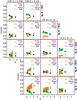 |
Fig. 8 As in Fig. 7, but for Cmocks. |
| In the text | |
|
Fig. 9 Slopes of the colour − density relation linear fits for the 23 Cmocks and the 23 Omocks for galaxies with MB ≤ −20 in the four redshift bins (label on the top), as in the third row of Figs. 7 and 8. Red and blue small diamonds: red and blue galaxies in each Omock; light purple and cyan small diamonds: red and blue galaxies in each Cmock. Red and blue big triangles: mean values of red and blue small diamonds, with the vertical error bar being the rms among all 23 mock samples. Light purple and cyan big squares: mean values of light purple and cyan small diamonds, with their rms. Orange and green circles: slope and its error for VVDS observed data (from C06) for red and blue galaxies, respectively. |
| In the text | |
|
Fig. 10 Slopes of the linear fits of the colour − density relation in each panel of Figs. 7 and 8, for fred on the left panel and fblue in the right panel. Lines and shaded areas: VVDS observed data with error. Triangles: Omocks. Squares: Cmocks. Different colours of lines and symbols are for the different luminosity thresholds, as indicated in the labels. In each redshift bin, delimited by vertical dashed lines, all points should be considered at the same (central) x-value, but they are shifted for clarity. |
| In the text | |
|
Fig. 11 Total halo mass as a function of the local density contrast computed in this work in different redshift bins (as in the labels) for galaxies with MB ≤ − 20. The values of the density contrast are indicated as log (1 + δ) in the bottom x-axis and as δ in the top x-axis. The halo is the FOF halo in which the galaxy reside (the halo of the group/cluster of which the galaxy is member). Four top panels: Cmocks. Four bottom panels: Omocks. Red circles and contours refer to central galaxies, blue squares and contours to satellite galaxies. Each panel includes all the 23 mock samples. Lines represent the isodensity contours of all the galaxies in the panel. For clarity, single galaxies are plotted as small dots only outside the lowest density contour. Filled red circles (/blue squares) are the median values in density bins for central (/satellite) galaxies. The error bars represent the 16% and 84% of the halo mass distribution in each density bin. On the right vertical axis of each panel, we show the typical virial radius (in h-1 Mpc) corresponding to the halo mass on the left vertical axis. |
| In the text | |
|
Fig. 12 Top panel. Slope of the linear fit of the fred-density relation (thick red lines) and of the fblue-density relation (thin blue lines) as a function of redshift in Cmocks. Only galaxies with MB ≤ −20 are considered. Solid line: slopes as found in the model, the same as in Fig. 10. Dashed and dot-dashed lines: slopes for two different assumptions about the colour distributions of satellite galaxies. We assume that centrals galaxies have the same colour as in the model, but now we assume that satellites are either all red (dashed line) or all blue (dot-dashed line). Bottom panel. Slope of the linear fit of the fred-density relation as a function of redshift in Cmocks, for three different assumptions about the colour distributions of central and satellite galaxies. Solid line: all satellites are red, and all centrals are blue. Dotted line: all satellites and centrals residing in DM halos with virial mass ≥ 1013 M⊙ / h are red, while all other centrals are blue. Dashed line: like the dotted line, but in this case the red centrals are those residing in DM halos with virial mass ≥ 1012 M⊙ / h. For this plot we use the 23 Cmocks together, and we keep fsat increasing with δ and decreasing with z as we find in the mock samples. |
| In the text | |
Current usage metrics show cumulative count of Article Views (full-text article views including HTML views, PDF and ePub downloads, according to the available data) and Abstracts Views on Vision4Press platform.
Data correspond to usage on the plateform after 2015. The current usage metrics is available 48-96 hours after online publication and is updated daily on week days.
Initial download of the metrics may take a while.