| Issue |
A&A
Volume 548, December 2012
|
|
|---|---|---|
| Article Number | A40 | |
| Number of page(s) | 14 | |
| Section | Interstellar and circumstellar matter | |
| DOI | https://doi.org/10.1051/0004-6361/201118700 | |
| Published online | 16 November 2012 | |
Nanostructuration of carbonaceous dust as seen through the positions of the 6.2 and 7.7 μm AIBs
1
Institut des Sciences Moléculaires d’Orsay, CNRS – Univ. Paris-Sud 11, UMR
8214,
91405
Orsay Cedex,
France
e-mail: This email address is being protected from spambots. You need JavaScript enabled to view it.
2
Institut d’Astrophysique Spatiale, CNRS – Univ. Paris-Sud 11, UMR
8617, 91405
Orsay Cedex,
France
3
Laboratoire de Géologie, École Normale Supérieure, UMR CNRS
8538, 75231
Paris Cedex 5,
France
Received: 21 December 2011
Accepted: 8 September 2012
Abstract
Context. Carbonaceous cosmic dust is observed through infrared spectroscopy either in absorption or in emission. The details of the spectral features are believed to shed some light on its structure and finally enable the study of its life cycle.
Aims. The goal is to combine several analytical tools in order to decipher the intimate nanostructure of some soot samples. Such materials provide interesting laboratory analogues of cosmic dust. In particular, spectroscopic and structural characteristics that help to describe the polyaromatic units embedded into the soot, including their size, morphology, and organisation are explored.
Methods. Laboratory analogues of the carbonaceous interstellar and circumstellar dust were produced in fuel-rich low-pressure, premixed and flat flames. The soot particles were investigated by infrared absorption spectroscopy in the 2−15 μm spectral region. Raman spectroscopic measurements and high-resolution transmission electron microscopy were performed, which offered complementary information to better delineate the intimate structure of the analogues.
Results. These laboratory analogues appeared to be mainly composed of sp2 carbon, with a low sp3 carbon content. A cross relation between the positions of the aromatic C=C bands at about 6.2 micron and the band at about 8 micron is shown to trace differences in shapes and structures of the polyaromatic units in the soot. Such effects are due to the defects of the polyaromatic structures in the form of non-hexagonal rings and/or aliphatic bridges. The role of these defects is thus observed through the 6.2 and 7.7 μm aromatic infrared band positions, and a distinction between carriers composed of curved aromatic sheets and more planar ones can be inferred. Based on these nanostructural differences, a scenario of nanograin growth and evolution is proposed.
Key words: astrochemistry / dust, extinction / ISM: general / infrared: ISM
Present address: Laboratoire de Physique des Lasers, Atomes et Molécules, CNRS – Univ. Lille 1 Sciences et Technologies, UMR 8523, 59655 Villeneuve d’Ascq Cedex, France.
© ESO, 2012
1. Introduction
Carbonaceous materials are observed throughout many different regions in space (Henning & Salama 1998; Ehrenfreund & Charnley 2000). The diverse environment conditions thus met for carbon chemistry lead to original questions dealing not only with the structure of these carbonaceous particles (e.g. their sizes, which range from (large) polycyclic aromatic hydrocarbon (PAH) molecules to solid-state carbon grains) but also their dynamics, such as internal energy transfer and relaxation (Puget & Léger 1989; Allamandola et al. 1989; Draine & Li 2001). These questions also address the formation and destruction of these particles during their life cycle. Although spectral features in the visible to UV range of wavelengths are observed and carried by carbonaceous materials (Désert et al. 1990; Draine 2003; Zubko et al. 2004), this fraction of cosmic dust is mainly observed through remote infrared (IR) spectroscopy. In particular, the mid-IR emission features observed in many astronomical objects (Gillett et al. 1973), often called the aromatic infrared bands (AIBs), trace carbonaceous particles of a few nanometers often attributed to PAHs in most of the astrophysical literature (Léger & Puget 1984; Crawford et al. 1985; Tielens 2008). Heated by UV and visible starlight, these nanoparticles emit through their vibrational bands thanks to an out-of-equilibrium process known as the transient heating mechanism (Puget & Léger 1989; Allamandola et al. 1989; Draine & Li 2001). These bands exhibit differences in shape and position in distinct astrophysical environments. Three main classes of astrophysical spectra have been proposed based on the observed spectral characteristics in the 6 to 9 μm wavelength region (Peeters et al. 2002). However, if the band positions in most sources are reminiscent of those of aromatic materials (Duley & Williams 1981; Goto et al. 2007), the exact nature of the emitters is unknown. It is expected that the spectral diversity of the bands will provide clues to the chemical and structural nature of the observed materials, which should allow one to specify their formation and evolution conditions in the interstellar medium. Another mid-IR spectral feature attributed to carbon-based materials is also observed in absorption at 3.4 μm and is attributed to hydrogenated amorphous carbon (a-C:H). Related bands at 6.85 and 7.25 μm are observed as well (Pendleton & Allamandola 2002; Dartois et al. 2004, 2005; Dartois et al. 2007; Dartois & Muñoz-Caro 2007; Sloan et al. 2007). This component is close to a polymer-like a-C:H (high content of hydrogen) and dominated by a sp3 hybridization. A link between the amorphous and the polyaromatic dust components is also expected, and different scenarios have been proposed. These are based on the photoconversion of the amorphous component (exhibiting saturated aliphatic hydrocarbon features) into the aromatic one (Goto et al. 2003; Sloan et al. 2007; Pino et al. 2008; Acke et al. 2010; Gadallah et al. 2011).
In order to study these materials, astronomical observations are ongoing (Goto et al. 2007; Sloan et al. 2007; Draine & Li 2007; Galliano et al. 2008). These are supported by many laboratory astrophysics works on various analogues in the form of pure or hydrogenated carbon materials. Various production techniques are used, such as laser pyrolysis (Schnaiter et al. 1999; Herlin et al. 1998; Reynaud et al. 2001; Galvez et al. 2002; Jäger et al. 2006), laser ablation (Mennella et al. 1999; Jäger et al. 2008), photolysis (Dartois et al. 2004, 2005), reactive plasmas (Lee & Wdowiak 1993; Scott & Duley 1996; Furton et al. 1999; Goto et al. 2000; Godard & Dartois 2010; Godard et al. 2011), and others (Jäger et al. 1999; Jäger et al. 2009; Biennier et al. 2009). At Orsay (France), our gas-phase chemical reactor is a low-pressure flame, flat and premixed. It is a model reactor for combustion studies as it provides a one-dimensional, time-resolved burning medium. It is not meant to mimic the reactive chemistry at work in the circumstellar environments or in the interstellar medium (ISM). Similar systems have been used to synthesize circumstellar dust analogues (Colangeli et al. 1995; Schnaiter et al. 1996). The produced soot was already shown to provide pertinent laboratory analogues of the cosmic dust (Pino et al. 2008; Brunetto et al. 2009). The soot particles are mainly composed of carbon and hydrogen, although oxygen is used as oxidizer. They consist of agglomerated primary particles with diameters of the order of 5−30 nm comprising organised, disordered, and possibly amorphous-like domains. The nanostructuration of the primary particles is described by the sizes, shapes, and organisations of the polyaromatic units. These polyaromatic unit sizes are of a few nanometers maximum (Vander Wal et al. 2007; Alfè et al. 2009) and are generally linked by an aliphatic component. The organised domains range from two to, typically, four stacked graphene layers (bi-periodic turbostratic order) that could be regarded as highly disordered graphitic lattices (Bockhorn 1994; Homann 1998; Dippel et al. 1999; Sadezky et al. 2005; Alfè et al. 2009). These stacked polyaromatic units form the basic structural units, the BSUs. This concept of BSU is at the core of the analysis of all polyaromatic materials. The global arrangement of these BSUs (orientation) and their proportion depend strongly on the soot itself and therefore on the burning conditions (Alfè et al. 2009). The cross-linked individual structural units give rise to the disordered carbon domains. It should be recalled that these individual polyaromatic units are called sp2 clusters in the literature related to amorphous carbon (a-C) because they strongly influence the electronic structure (Robertson & O’Reilly 1987).
In this study, we show that our reactor is capable of producing a structural and chemical variety of materials under controlled conditions. The diagnostics used are Fourier transform infrared absorption (FTIR) and Raman spectroscopies of the collected solid particles. High resolution transmission electron microscope (HRTEM) images were taken to guide and confirm the analysis. The data are compared to the previous studies and discussed in the astrophysical context. In particular, the laboratory and astronomical IR spectral features are tentatively interpreted in the light of the soot structures.
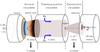 |
Fig. 1 Schematic view of the experimental set-up “Nanograins”. The burning region, the extraction cone in quartz, and the jet expansion region where the soot samples are collected by insertion of a KBr window can be seen. |
2. Experimental methods
2.1. Experimental set-up and soot production
Soot samples were produced at the Institut des Sciences Moléculaires d’Orsay (France). In the set-up, schemed in Fig. 1, a low-pressure flat burner provides flames of premixed hydrocarbon and oxygen gas. The flame is a one-dimensional chemical reactor offering a broad range of combustion conditions and sampling. Three typical samples, labelled hereafter sample 1−3, were produced with the aim to vary the aromatic to aliphatic CH bonds ratio and thus explore different kinds of interstellar carbonaceous analogues.
The source chamber contains a 60 mm diameter flat burner (McKenna model). The fuel was either ethylene (samples 1 and 2) or propylene (sample 3). It was premixed with oxygen before flowing through the burner at a controlled flow rate (4, 3.5, and 3 l/min for samples 1 to 3, respectively), and the rich C/O ratio was set to 1.6, 1.4, and 1.1 from samples 1 to 3, respectively. In the source chamber, the pressure was maintained at 80, 40, and 70 mbar for samples 1 to 3, respectively, by continuous pumping. Adjustments of all these parameters gave combustion regimes that produce different soot particles. The by-products were then extracted by a quartz cone inserted into the flame at a controlled distance from the burner. The particles diffused through a thermalization chamber in copper at a pressure of a few millibars and expanded into the vacuum (a few 10-2 mbar) through a 10 mm diameter nozzle. The soot was then deposited on a rotating KBr substrate window directly inserted into the molecular flow. The obtained thickness was typically in the 1−3 μm range, depending both on the production rate and the exposure time, and was rather homogeneous due to the off-axis rotation of the window during the deposition.
Observations.
2.2. Soot measurements
Samples 1 and 3 were characterised at the Institut d’Astrophysique Spatiale (Orsay, France) by FTIR spectroscopy using a Bruker 80v spectrometer, and sample 2 by FTIR microspectroscopy using a Nicolet Magna-IR 560 ESP spectrometer coupled to a Nicolet Nicplan IR microscope. Typically 128 scans or more (at 2 cm-1 resolution) were acquired in order to optimize the signal-to-noise ratio.
Samples were also characterized by Raman spectroscopy performed at the Laboratoire de Géologie de l’École Normale Supérieure (Paris, France) on a Renishaw inVia microspectrometer equipped with an Ar laser source, focused through a Leica microscope. The continuous Ar (514 nm) laser beam was used as exciting radiation. Care was taken to avoid modification of the carbon structure due to laser-induced heating effects. This is indeed confirmed by the fact that collecting several Raman spectra of the same soot sample at several laser fluence values did not reveal any visual and spectral modifications. The acquisition time was 10 or 60 s while the beam power was set to 0.2 mW and focused in a ≈1 μm spot (≈25 kW cm-2). The Raman shift was measured between 200 and 4000 cm-1.
The HRTEM images were acquired on a JEOL 2011 electron microscope operating at 200 kV using a LaB6 filament (0.144 nm resolution in the lattice fringe mode). A Gatan Orius SC100 CCD camera was used, and 4008 × 2672 pixels images with 256 gray levels were recorded. In the images recorded at 500 000 × magnification, the fringes represent the profile of the polyaromatic layers. The samples were deposited on an amorphous carbon lacey covering a copper mesh. The protocol was to make a suspension of soot agglomerates from that deposited on the window for IR and Raman diagnostics in an ethanol solution, put a drop of the suspension onto the grid, and let the ethanol vaporize. Preliminary measurements of soot sampled by inserting the grid directly in the molecular flow or using this protocol did not reveal evident alteration of the soot structure. A typical image at low magnification of a soot agglomerate transferred on the carbon lacey is shown in Fig. 2.
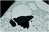 |
Fig. 2 Typical transmission electron microscope images at the 500 × magnification of a sample deposited on the carbon lacey after evaporation of the suspension of soot grains in ethanol. |
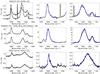 |
Fig. 3 Three astronomical spectra illustrating the different classes A to C (from top to bottom, respectively). The sources names are reported. On the left panels, the upper spectra are before and the lower ones are after continuum subtraction. On the other panels, the Gaussian fits (blue) are superimposed on the zoom of the spectra to show the details of the 6.2 and 7.7 μm band spectral region. |
3. Astronomical spectra of interstellar carbonaceous dust
A selection of astronomical data covering the 5 to 10 micron range was performed in order to extract spectral characteristics of the 6.2 and 7.7 μm AIBs. Short wavelength spectra (SWS) from the Infrared Space Observatory (ISO; de Graauw & et al. 1996) database1 were taken. These SWS spectra were retrieved using the pipeline processing version OLP10.1. A selection based on the highly processed data products (HPDP) (Sloan et al. 2003) was made, and individual orders were stitched by applying slight gain corrections (typically less than 10%) using wavelength overlaps. In addition, IR spectrograph (IRS) spectra, from the Spitzer satellite (Houck et al. 2004) were added. These IRS spectra were retrieved from the Spitzer archive2. The post-BCD (basic calibrated data) pipeline processed spectra were used, and as for ISO spectra, individual orders were stitched by applying slight gain corrections (typically less than 10%) using wavelength overlaps. Table 1 summarizes the log of the observations. This covers the three main classes of the observed astrophysical AIB spectra (Peeters et al. 2002; van Diedenhoven et al. 2004), the classes A, B and C.
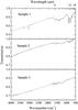 |
Fig. 4 Infrared transmission spectra, as recorded, of soot samples produced under various conditions (see text for details). Note that the CH stretch bands around 3000 cm-1 vary strongly, tracing different hydrogenation of the carbon skeleton, and that the continuum to band ratios are also different between sample 1 and the two others. In grey, the fitted continua are superimposed. |
Spectral characteristics of the bands were extracted by fitting the 6.2 and 7.7 micron bands with a set of three Gaussian bands, one for each of the 6.2, 7.7, and 8.6 micron AIBs, added by a local continuum baseline (Fig. 3). For the 6.2 micron AIB, the Gaussian was an asymmetric one to better fit the profile. The position around 8 micron was extracted using a single Gaussian in order to better compare the astronomical data to the laboratory data, instead of the usual set of two Gaussian or Lorentzian used in the analysis of astronomical data for this complex AIB. The goal was to probe the relation between the position of two AIBs, namely the 6.2 and 7.7 micron ones. Such a relation has already been reported (Peeters et al. 2002; Szczerba et al. 2005; Acke et al. 2010).
Vibrational band assignments measured in the absorption spectra of samples 1 to 3.
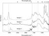 |
Fig. 5 IR absorption spectra of the three soot samples after continuum subtraction. An offset has been added for visual convenience. The spectra were normalized altogether in order to match the intensity of the band at 1600 cm-1. CO2 spectral contamination at about 2400 cm-1 for sample 2 and H2O spectral contamination in the 1800−1400 cm-1 range for sample 3 may be seen due to slight variations of the purge of the spectrometer. The vertical dotted line are centered on 3040, 1610, and 1250 cm-1. |
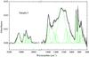 |
Fig. 6 IR absorption spectrum of sample 2 after continuum subtraction (grey curve). The deconvolution of the spectrum obtained by a sum of Gaussian bands is shown in black, together with the individual Gaussians in green. |
4. Soot analysis
4.1. Infrared spectroscopy
Infrared transmission spectra of the three selected soot samples are presented in Fig. 4. They illustrate the wide variety of materials that can be produced by tuning the burning conditions. An underlying continuum is observed, increasing with the photon energy, and the band-to-continuum ratio depends on the sample. The bands are relatively strong in the spectrum of sample 1, but the continuum largely dominates in all samples. We ascribe the continuum to low-lying electronic transitions, while the superimposed bands are attributable to vibrational transitions. A closer look reveals the presence of weak interference fringes as a weak modulation of the continuum. These are interference patterns on the transmitted IR beam within the samples that were homogeneous enough to behave like films. Other samples (not shown here) did show a stronger fringe pattern. Fits of the continuum (and fringes) were performed and subtracted to obtain the pure vibrational absorption spectra. These are shown in Fig. 5 and reveal the richness of the vibrational bands.
The band assignments are based on literature data for a-C:H (Bounouh et al. 1995; Ristein et al. 1998; Dartois et al. 2005), soot (Galvez et al. 2002; Santamaría et al. 2006) and natural carbonaceous materials such as coals (Ibarra et al. 1996; Geng et al. 2009). The region around 3000 cm-1 corresponds to the CH stretching modes, the one around 1600 cm-1 to the C=C (sp2) stretching modes, the one between 1500 and 1000 cm-1 to the CH bending and C-C (sp3) stretching motions with some contributions of sp2 C=C modes, and finally the 1000−720 cm-1 region corresponds to the CH “out-of-plane” (wagging) bending motions. The bands and their assignments are listed in Table 2 for each sample. These were obtained by a deconvolution of the spectra with a sum of Gaussian profiles. Some spectral characteristics were constrained in order to provide a consistent fit of all samples, in particular in congested regions. However, it is clear that the fit is not unique and the choice was guided by the possible assignments. In particular, the contribution from oxygen contamination was considered as minor regarding the weak carbonyl C=O contribution at about 1720 cm-1. The result of the deconvolution is shown in Fig. 6 in the case of sample 2, which exhibits all bands. The same set of Gaussian bands was used for the three spectra, and the constraints were identical: the positions were allowed to vary around the observable bands and the full widths at half maximum (FWHMs) were allowed to vary within the same ranges of values used in Pino et al. (2008).
The CH stretching mode analysis led us to label our soot according to the relative intensities of the aromatic sp2 CH and the aliphatic sp3 CHn=2−3 stretching modes. Sample 1 has mainly aromatic CH bonds, sample 3 sp3 CHn=2−3 bonds, and sample 2 has a mixture of both. Their varying ratios and the related changes of the precise position of the band at 1600 cm-1 was inferred to be related to the intimate insertion of the polyaromatic units into a cross-linking aliphatic network in soot (Pino et al. 2008). As can be seen from Table 2, the band position of the aromatic C=C stretch moves from 1611 down to 1585 cm-1, from sample 1 to 3, while the CH ratio Rarom equals 0.87, 0.49, and 0.09 respectively. This is consistent with the results found in Pino et al. (2008). In addition, a detailed analysis of the CH stretch region at about 2900 cm-1 shows that tertiary aliphatic CH is a weak feature. The band is probably dominated by the CH2 band contribution, which appeared to broaden upon environmental constraints. This result is consistent with the IR analysis in typical a-C:H samples (Bounouh et al. 1995; Dartois et al. 2005).
The most congested spectral region ranges from 1600 to 1000 cm-1. The fitting procedure is used only to extract the positions of the vibrational bands. Actually, quantitative information on the other spectral characteristics are difficult to derive for two main reasons: the continuum level and thus the subtracted baseline are poorly constrained in this region, and the broadness of the vibrational bands themselves produces strongly congested IR spectra. For instance, it was shown that in pure amorphous carbon the proportion and organisation (stacking) of the aromatic sp2 C strongly affect the activity of the aromatic skeleton bands. The more sp2 over sp3 coordination in disordered carbons, the more IR active are the bands involved in this spectral region. This was shown to result in two very broad components centred at about 1580 and 1300 cm-1 in amorphous carbon (Thèye et al. 2001; Rodil et al. 2002; Rodil 2005). In the three soot samples, such a contribution may also be expected.
Apart from the position of the band at 1600 cm-1, the main difference between the three samples is the absence (for sample 1) or presence of a feature in the range 1270−1200 cm-1 for samples 2 and 3. This band is first assigned to sp3 C-C stretch, and the marked absence in the absorption spectrum of sample 1 would suggest that the sp3 carbon content of this soot should be lower. It is consistent with the relative weakness of the sp3 CHn=2−3 stretch bands. Apparent intensity ratios between the band at 1600 cm-1 and the band at about 1250 cm-1 also suggest that the sp3 content is higher in samples 2 and 3. A rough evaluation of the apparent aromaticities fa = 1−Cal/C, where Cal/C is the aliphatic carbon fraction, can be deduced from the intensities of the aliphatic CH stretch bands and the aromatic C=C band around 1600 cm-1. Such a method only probes sp3 carbon bound to hydrogen. Band strengths that were used are taken from Dartois et al. (2007), and fa is found to be close to 1 for all samples. It shows that the measurable true amorphous sp3 phase of the soot samples is a minor component. Such a small concentration of sp3 C in the three samples does not solely explain the activation of the band in the range 1270−1200 cm-1 in samples 2 and 3. Following the attribution of the 1600 cm-1 band variation, a large part of the activity of the band at about 1250 cm-1 in samples 2 and 3 is assigned to involve the defects at the edges or within the polyaromatic structures. According to this assignment, the band found in the 1200 to 1270 cm-1 range is called the defect band for all our soot samples. The defects at the edges are in the form of aliphatic bridges (the cross-linkage) in the place of peripheral H. The defects within the aromatic sheet arise in the form of non-hexagonal rings. Both types of defects are made up with sp3 carbon atoms, consistent with the defect band position typical of that of sp3 C-C stretch.
The bands at about 1445 and 1380 cm-1 exhibit also strong differences. In the case of samples 2 and 3, assignment to the CHn=2−3 bending motions is straightforward. In the case of sample 1, their spectral characteristics are slightly different and their intensity relative to the surrounding spectral bands is clearly stronger. The band at 1445 cm-1 involves aromatic C=C stretching mode, and the mode giving rise to the 1380 cm-1 band is attributed to CH3 bending motion.
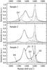 |
Fig. 7 First-order Raman spectra of the soot samples (in gray). The baseline was subtracted and the spectra were normalized to the peak amplitude of the G band. The fit were performed using a sum of 4 Lorentzians (or 5) plus 1 Gaussian (in black). The individual band assigments are indicated for sample 3, but are the same for all samples. The band D1′ was added for a better fit of sample 1 spectrum. |
The intensity ratio of the out-of-plane aromatic CH bending modes below 1000 cm-1 also varies. The different aromatic bands are connected to the number of adjacent H attached to the same aromatic cycle. The solo (at about 884 cm-1) to quartet (at about 759 cm-1) intensity ratio is close to one for sample 1, whereas the solo mode dominates this spectral region in sample 3. This spectral characteristic is generally considered to be related to the extent of the polyaromatic units. It apparently shows that the mean size of the polyaromatic units is bigger in samples 2 and 3 than that in sample 1. In a study complementing IR absorption spectroscopy and HRTEM on soot produced by laser pyrolysis, it was shown that the out-of-plane intensity ratio was directly related to the mean size of the polyaromatic structures (Galvez et al. 2002). Using this relation, the mean diameter would be 1.3−1.4 nm, indicating polyaromatic structures of typically 60−80 carbon atoms in the soot particles of sample 1. Such values should be taken carefully but may be considered as a good indicator of a minimum value due to the image analysis protocol (Galvez et al. 2002). Using the CH to CC aromatic stretch integrated absorbance, a rough estimation leads to an aromatic Car/Har within 4−14 for sample 1. Such values imply polyaromatic units of 100 carbon atoms or more. The discrepancy may come from absolute band strengths of the C=C stretch, which is known to be sensitive to the environment (heteroatoms (Ibarra et al. 1996) and/or stacking (Thèye et al. 2001; Rodil et al. 2002; Rodil 2005)). In the case of samples 2 and 3, the use of the relation proposed by Galvez et al. (2002) leads to polyaromatic unit sizes beyond 2 nm, i.e. in the range 100−200 carbon atoms at least.
Substitution at the edge of an individual polyaromatic unit is known to influence the out-of-plane bending modes. Historically, it was used to identify the solo, duo, trio, and quartet nature of the modes by changing the substitution pattern (Socrates 2001). Within the soot, substitution is, at the molecular level, done by the aliphatic component that cross-links the aromatic units. In a strongly cross-linked network, the out-of-plane bending modes should reflect this characteristic more than a close relation to the polyaromatic unit size distribution. In the case of samples 2 and 3, the evolution of the aromatic out-of-plane wagging CH bands should primarily be influenced by such cross-linkage.
4.2. Raman spectroscopy
The first-order Raman spectra in the 900−1900 cm-1 region are shown in Fig. 7. These spectra were continuum subtracted. Only that of sample 1 was clearly showing some electronic fluorescence underlying the bands. These spectra reveal the typical G and D band structure of disordered carbonaceous materials (Ferrari & Robertson 2000; Beyssac et al. 2003). The analysis was performed following the procedure proposed by Sadezky et al. (2005) for soot and was already successfully applied to some of our soot samples (Brunetto et al. 2009). The characteristics and assignments of the bands are listed in Table 3. The G band relates to the aromatic sp2 C=C stretching mode. The D1 band is assigned to in-plane (edge) defects. The D3 band is assigned to the presence of defects (in plane) or amorphous sp3 carbons network that strongly affect the sp2 C=C stretch positions. The D2 band was tentatively assigned to involve an aromatic C=C stretching mode in polyaromatic units not belonging to a BSU (the organised domain) or at the surface of it and also to the variation of the distance between the graphene units (Dresselhaus & Dresselhaus 1982). The D4 band was shown to be related to the sp3 C content (Schwan et al. 1996) or was either assigned to polyenic-like sp2 C=C stretching motions (Shirakaw et al. 1973) or more vaguely to mixed sp2-sp3 CC motions (Bacsa et al. 1993; Dippel et al. 1999) because of the similarities to the Raman spectra of polyenes. The second-order Raman spectra in the 2200−3600 cm-1 region are shown in Fig. 8 together with a simple deconvolution. This was done using only three Lorentzian bands tentatively assigned to the 2*D1, G+D1 and 2*G bands. A contribution of weaker bands in this congested region cannot be excluded but, due to the large width of the bands, these were not included.
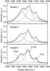 |
Fig. 8 Second-order Raman shift of the soot samples (in gray). The baseline was subtracted and the spectra were normalized to the peak amplitude of the G band. The fit was performed using a sum of 3 Lorentzians (in black). The individual bands are indicated for sample 3, but are the same for all samples. |
In the case of sample 1, the D1 region was deconvoluted adding an extra D1′ band to better fit the experimental data. The D1 is located at about 1372 cm-1 and the band D1′ at about 1269 cm-1. Regarding the assignment of the D1 band, it was shown that this band could originate from the merging of subbands characteristic of the individual polyaromatic subunits. The merging depends on their insertion: the more cross linked, the more merged (Negri et al. 2002). In the present case, the substructure of the D1 band may thus suggest the presence of mostly polyaromatic units poorly linked together as the intimate soot structure. The weakness of the D3 band typical of true amorphous carbon, i.e. a random mixture of sp2 and sp3 carbons, also suggests that the soot contains mainly sp2 carbon. Overall, the spectrum points to a poor level of organisation of the polyaromatic units, as inferred by the ratio of the area of the G and D1 bands, and the relatively large FWHMs.
Spectral characteristics of the deconvoluted bands of the Raman spectra of the three soot samples.
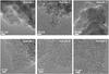 |
Fig. 9 Selected HRTEM images of samples 1 to 3. The upper ones show the primary particle structures of the soot samples at a magnification of 50 000 × . The lower images show nanostructural details at a 500 000 × magnification of primary particles, the stick illustrating a 2 nm length. These were measured on the thinnest border (below 10 nm) of some grains. |
Spectral parameters or structural observables obtained from the different diagnostics.
In the case of sample 2, the D1 band is clearly stronger than the G band (Table 3). However the bands remain narrow compared to amorphous carbon, indicating a disordered carbon rather than a true amorphous carbon, although there is a clear appearance of the D3 band. The spectrum thus reveals that the sp2 carbon content is still rather high in this soot. The Raman spectrum of sample 3 resembles that of sample 2, with the AD1/(AG + AD2) band integrated area ratio and the D3 band area being slightly stronger. Thus sample 3 might have a similar carbon skeleton to that of sample 2. All spectra show the presence of a D2 band, illustrating that the number of coherent domains should be low in these materials. However, the deconvolution of the D2 band is poorly constrained and only the sum AG + AD2 and the position of the G band are considered throughout the present study.
Following the three-stage model proposed by Ferrari & Robertson (2000), all three soot samples belong to stage 2, i.e. on the transition from nanometer-size graphitic structures to amorphous carbon. Considering the G peak position, at about 1600 cm-1, and the AD1/(AG + AD2) ratio, the soot samples may be considered as made of nanometer-size polyaromatic structures with a rather low content of sp3 carbon, as usually observed in soot (Alfè et al. 2009). It should be noted that no attempt to extract a mean length from AD1/(AG + AD2) integrated area band ratios is performed. For such small and disordered polyaromatic units, it was shown that a good spectroscopic parameter cannot be built from first-order Raman bands only (Bernard et al. 2010; Larouche & Stansfield 2010).
4.3. HRTEM images
The organisation of the soot samples was analysed at the nanometer scale by HRTEM. A selection of the images is shown in Fig. 9. The images were taken on the border of the grain agglomerates in order to explore the nanostructuration of a single primary particle composing the soot samples. A qualitative analysis was performed by comparing the images. The sizes of the primary particles range from a few nanometers to about 30 nm in diameter. Samples 1 and 2 show mostly small particles with irregular shapes, while sample 3 is generally made up of bigger ones that are more or less spherical (upper images in Fig. 9). Such behaviours are generally connected to the degree of maturity of the soot and its growing sequences. Sample 1 would be considered as a young soot. Sample 2 has experienced more growth by surface accretion and perhaps more ageing. However, the high-resolution images where fringes can be seen (lower images in Fig. 9) exhibit poorly organised polyaromatic units (the fringes) with little regions arranged in coherent domains. In mature soot, these BSUs are generally concentric and parallel to the surface of the primary particles, while (many) secondary centres in young soot, when seen, probably trace the initial structures of the seeds that coalesced from a tar-like dispersed medium to form the soot primary particles (Alfè et al. 2009). All three soot samples are, in fact, far from being mature.
In sample 1, the polyaromatic units are about a few nm long maximum. Some are apparently stacked into BSUs (Rouzaud & Oberlin 1989), although these do not dominate their arrangements. They are observed to form a fairly concentric organisation. Some fullerene-like structures, appearing as more or less circular fringes, may be seen. In sample 2, the polyaromatic units are about the same size but tortuosity is in fact clearly observable. More fullerene-like structures may even be found in the images while far fewer BSUs are seen. In addition, presumably in relation to the shape of the units, many secondary nuclei can be found, which results in the irregular shape of the primary particles. In sample 3, the curvature is more evident than that of sample 2 with even fewer BSUs. Numerous fullerene-like structures are found and many local concentric fringes can be seen closer to those of sample 1. Overall, disorder dominates in all samples. The main differences seem to arise from the curvature of the polyaromatic units and the reminiscence of the presumed seeds of nucleation.
5. Astrophysical implications of the nanostructuration
5.1. The role of defects for the 6.2 and 7.7 micron AIB positions
The use of the three complementary diagnostics enables one to infer more detailed information about the size, morphology, and organisation of the polyaromatic units within the soot samples. This gives the opportunity to build reliable spectroscopic parameters based only on IR spectral characteristics in order to better understand the relation between the structure of the carbonaceous particles and the circumstellar and interstellar IR emission bands. For instance, the 6.2 μm band was shown to trace some evolution of the carbonaceous material (Pino et al. 2008). The band position is related to the aromatic CH to aliphatic CH stretching band ratio. The effect was clearly pointing to the substitution level on the polyaromatic units. The influences of the sp3 to sp2 ratio, size, morphology, and organisation were not clearly identified. We attempted to address these points in the light of the present multi-diagnostic study. A summary of the observables is listed in Table 4.
In the case of sample 1, IR and Raman studies converge towards a soot mainly made of nanometer-size polyaromatic structures with hydrogen at their boundaries, poorly linked together by a few and probably short aliphatic carbon bridges. Reminiscence of the spectra of the individual PAHs, which are elemental bricks forming the polyaromatic structures of the carbon skeleton, may be seen in the Raman spectra. Such interpretations are well confirmed by the HRTEM studies on sample 1. In the case of samples 2 and 3, the polyaromatic units are progressively poorly hydrogenated and increasingly cross-linked by aliphatic bridges. This is consistent with HRTEM images, which show that polyaromatic units dominate the structure and truly amorphous domains are absent. Stacking is not observed to be significant, and most of the polyaromatic units are not found to belong to coherent domains regarding the HRTEM images (Fig. 9). It may also be deduced from the rather large bandwidths of the Raman bands and even from the merged G and D2 bands (Fig. 7).
Raman spectra are often used to estimate the mean size of the aromatic units, following the work of Tuinstra & Koenig (1970) and the extensions as rationalized by Ferrari & Robertson (2000). Many attempts to derive analytical formulation of size dependence have been published (Cancado et al. 2006). However, it is clear that no valuable conclusion may be obtained for disordered materials (Bernard et al. 2010). In fact, spectroscopic parameters employing second-order Raman bands have been built to include the effect of tortuosity as well. In particular, the 2*D1 band (the overtone of the D1 band) was shown to provide some useful information through its bandwidth (Lespade et al. 1984; Larouche & Stansfield 2010). In our samples, the 2*D1 bandwidth goes from about 300 down to 230 cm-1 for samples 1 to 3 (Table 3), respectively, implying average plane length of 2 nm or below using Larouche & Stansfield (2010). Therefore, IR and Raman diagnostics converge towards polyaromatic units with a mean size of 1−2 nm maximum for all samples, which is qualitatively consistent with the HRTEM images.
The main differences revealed by the HRTEM images point to the tortuosity of the aromatic units, or even their curvature. It was shown that, depending on the flame conditions, flat to strongly curved native nanoparticles may be produced (Violi 2004). Curvature due to the presence of defects, such as pentagonal rings, within the polyaromatic unit leads to spherical structures, while perfectly hexagonal graphene sheet can form only tubular-type curvature (Gupta & Saxena 2009). Tortuosity is associated with reticulation due to small aliphatic bridges that link different polyaromatic units. The tortuosity and curvature can be deduced from the characteristics of the bands in the first- and the second-order regions of the Raman spectra. Larouche & Stansfield (2010) proposed a parameter called tortuosity ratio, RTor, which somehow quantifies the effect of tortuosity and curvature in the graphitic layers in order to extract an equivalent length for curved graphitic layers. This parameter RTor is defined as:  (1)where A is the integrated area of the bands and D(λ) is a normalization parameter that depends on the laser wavelength. When curvature increases with no defects, RTor increases because curvature enhances the 2*D1 band intensity compared to that for mostly planar graphene layers (Larouche & Stansfield 2010; Gupta & Saxena 2009). If the number of defects is increasing, RTor decreases. According to the present data, RTor is found to decrease from sample 1 to 3, although curvature is seen to be present in the HRTEM images and from the Raman band positions (Table 3). It suggests that the number of defects is presumably higher in samples 2 and 3 than in sample 1, as suggested by the defect band in their IR spectra.
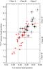 |
Fig. 10 Evolution of the position of the defect band at about 8 μm versus that at about 6.2 μm. Black dots: experimental data extracted from a sample of soot. These belong to the same sample that was used in Pino et al. (2008) and only those exhibiting a clear defect band were chosen, as may be seen in samples 2 and 3. Red triangles: observational data extracted from a sample of astrophysical objects. The region of the different AIB classes for each bands are shown, as defined in Peeters et al. (2002). |
In astronomical observations, this means that the class C spectral characteristics are pointing out carriers made of polyaromatic units with many defects. Moving to class A spectral features, emitters involve more planar polyaromatic entities with much less cross-linkage. Defects within the aromatic skeleton cannot be excluded for these ones either, because specific spectral features of non-hexagonal rings are not known yet but could participate in the 7.7 μm AIB complex band. Thus the 6.2 and 7.7 μm AIB positions are found to trace the shapes of the polyaromatic nanostructures of the carrier rather than the size of the units.
5.2. Evolutionary scenarios based on the 6.2 and 7.7 μm AIB position variations
Evolutionary scenarios that attempt to decipher the life cycle of dust are usually tentatively linking the different components that are observed in different regions. In particular, connecting the amorphous component observed in absorption in the diffuse medium to the aromatic one observed through the AIBs remains a challenge. The key work of classifying the AIBs into three main classes (Peeters et al. 2002) has shed new light on the aromatic components in space, revealing some important variations. In addition, the spatially resolved observations of the CH band regions in few objects, mainly those that may give rise to the class B and C carriers of the AIBs (Goto et al. 2003, 2007), have clearly triggered some new thought. More and more, an interplay between aliphatic and aromatic component is outlined, and the main astrophysical linking ingredient is supposedly the harsh UV irradiation (Goto et al. 2003; Bréchignac et al. 2005; Goto et al. 2007; Sloan et al. 2007; Pino et al. 2008; Acke et al. 2010). In Pino et al. (2008), we have shown that a smooth variation of some spectral characteristics from class C to A can be reproduced by a large sample of soot produced in sooting flames. It was suggested that the progressive modification of the emitting carrier, in particular its aliphatic to aromatic ratio, was at the core of such evolution. However, we show here that sample 3 and sample 2, which provide good laboratory analogue for class C carriers, are dominated by the aromatic component. Thus, the AIBs seem to be emitted by materials that contain a low proportion of aliphatic carbon, which may still be seen through the CH stretching and bending modes. It is thus more the role of the defects that seems to be at work and gives rise to different nanostructurations, rather than sp3 domains embedded in the soot particles.
This effect is consistent with the observation of a correlation of the 6.2 and 7.7 μm band position in space, these shift from 6.3 (8.2) down to 6.2 (7.7) μm from class C (C′) to class A (A′), respectively (Peeters et al. 2002). The nomenclature given by Peeters et al. (2002) for each band has been reproduced here and was used to define the three main classes. In Fig. 10, we report this correlation for a sample of soot. These soot samples were used for showing the correlation between the relative abundance ratio of aliphatic CH and aromatic CH bond and the position of the 6.2 μm band (Pino et al. 2008), added by samples 2 and 3. Soot resembling sample 1 do not exhibit the defect band and was thus not included. Astronomical data covering the full range spanned by the positions, i.e. from class C to A, are superimposed. Again, a similar tendency is observed between laboratory and observational spectral characteristics, although the laboratory data are dominated by class B and C soot types while astronomical data contain few C class type sources. The absence of a good laboratory analogue exhibiting a band at 7.7 μm currently precludes a careful assignment of the band to possible defect-like modes. It is noteworthy that the emission mechanism at work hinders the observation of emission in the mid-IR from the soot-like or amorphous grains (where the carriers of the class A AIB are observed), in the stellar outflow, thanks to the stochastic heating (Pino et al. 2008).
A short tour into the actual soot growth and ageing knowledges is necessary in order to draw some scenario for carbon dust growth. Combustion is not meant here to represent any astrophysical media reaction pathways, but represents the best studied reactive medium that produces nanoparticles with different nanostructurations in the laboratory. In sooting premixed flames, the soot is formed in a region where oxidation is almost hindered and conditions may be roughly described as pyrolytic ones with a slowly decreasing temperature. Inception is the main actual problem, and the nuclei arise from different mechanisms: aggregation of the PAHs to form dimers and bigger clusters (Miller et al. 1985) or acetylenic chain polymerisation that may further rearrange into aromatic units within the primary particles of the soot (Krestinin 1998). A driving force between these scenarios is the role of chemical condensation, as opposed to physical condensation, which involves pure van der Waals forces for the formation of the PAH clusters. Experimental evidences for the implication of reactivity between the molecules that compose the carbonaceous precursors (chains or PAHs) are more and more observed and predicted (Homann 1998; Violi et al. 2005; Chung & Violi 2011). Actually, the scenarios that dominate the combustion literature all involve PAHs, but have been recently rationalized into two main paths. One is based on the growth of large peri-condensed PAHs (PCAHs). The other involves branched smaller polyaromatic units forming oligomers, which are called aromatic-aliphatic linked hydrocarbons, the AALHs (D’Anna 2009; Homann 1998). After inception, mass growth is governed by coagulation of the nuclei and surface accretion of the gas-phase molecules (PAHs and chains). Their respective efficiency depends on the relative abundances. The nuclei retain (partly) their structure and are indeed observed in sampled soot (Alfè et al. 2009). When soot ageing (maturation) takes place, accompanied by surface accretion, a (large) crust of polyaromatic units organised into BSUs is formed and grows. It leads to concentric and stacked units parallel to the nanoparticle surface, with a more disordered core containing the nuclei. This scenario is clearly oversimplified, and even the nature of the nuclei is an issue, from strongly aliphatic to strongly aromatic. The nanostructuration of mature soot is more consensual. Such a scenario relies on understanding of the different steps of growth, depending on the stock of gaseous carbon molecules. It implies that all steps may be traced by different nanostructures within the soot, which somehow add up. Indeed, nanostructuration usually retains a memory of formation conditions. Thus, the structures observed here and their spectral features revealed that the sampled soot experienced different growth events that add together, rather than successive transformations of the intimate structure.
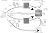 |
Fig. 11 Possible scenarios of the growth and evolution of the nanograins from a structural point of view, as sketched from the spectral variations of the IR bands. The possible role of UV irradiation in connecting different molecular assemblies and structures is underlined. This scenario is aimed at emphasizing the filiation between different nanostructures. In this scheme, the nomenclature at the top refers to all structures drawn below, for example, the polyaromatic dust comprises the soot particles, the PAH-like, the fullerenes and the mature AALHs photodesorbed species. The AALH and the soot particles are supposed to carry the class B and C AIBs. The class A could be emitted by PAH-like species and/or the mature AALH species. HACA refers to hydrogen abstraction and acetylene addition. The red squares on the primary particles images delimit the reminiscent soot nuclei. |
Such a growth and evolutionary scenario may be transposed to carbonaceous dust, and insights into the nanostructuration may be deduced from the IR emission spectrum. In Fig. 11, a scheme illustrating the two dominating routes to form polyaromatic dust is represented together with the possible role of the UV irradiation. The route to the hydrogenated amorphous carbon, the a-C:H component, is also reported through a chemical condensation mechanism. The horizontal arrow is taken as the time that traces growth and evolution (ageing) of the grains altered by UV or cosmic ray irradiations. Such a scheme is adapted from that drawn in combustion science (D’Anna 2009). An interplay between both aromatic routes occurs depending on the conditions. Chemical condensation of the gaseous hydrocarbon molecules may form the nuclei. These would contain, at some stage, small polyaromatic units including some defects (reticulation or curvature due to pentagonal rings for examples, like the AALHs). These could allow the formation of fullerenes, which were recently discovered in space (Sellgren et al. 2010; Cami et al. 2010), when pentagonal cycles can be preserved and isolated. Then growth of more planar polyaromatic units on the surface of these nuclei may occur. These would lead to the smooth evolution of the class C to B, following the evolution from nuclei to (solid) polyaromatic dust. Class A species would thus either (or more probably the interplay of both) be due to photodarkening of the nanograins by the harsh UV radiation followed by photodesorption or to the heterogeneous reactions that would produce large PAH-like species in the gas phase. Recent experiments have given evidence that heterogeneous reactions occur in some flames when soot inception has occurred, leading to the appearance of much larger PAHs in the gas phase (Faccinetto et al. 2011). The alteration of the a-C:H component could also link this component to the polyaromatic dust, presumably via photodarkening. In this scheme, it should be noted that the nanostructuration of the class A emitters remains poorly characterised, but is proposed to range from mature AALHs to PAH-like species.
6. Conclusion
A detailed analysis of three soot samples produced under various burning conditions has been performed by complementary studies using IR absorption and Raman spectroscopies. HRTEM images were shown to support the spectral analysis and interpretation of the soot nanostructures, i.e. the size, shapes and organisation of the polyaromatic units of such aromatic materials. All diagnostics are shown to be at their limit of (quantitative) interpretation due to the disordered nature of the material and the nanometer sizes of the polyaromatic units composing the soot primary particles. The polyaromatic unit sizes escape most of the (mostly empirical) formulations linking the size to a spectroscopic parameter that may be found in the literature. However, the cross-analysis allows us to constrain the possible interpretation of the spectral features variations. In particular, the central role of defects has been pointed out. The term defects is used because the primary particles are mainly composed of aromatic sp2 carbon, while the defects involved mainly sp3 (or mixed sp2-sp3 for non-hexagonal cycle) carbon, rather than being composed of a sp3 carbon network embedding the aromatic carbon. Their role is mainly seen in the tortuosity and curvature in the HRTEM images. The defects are mostly located at the edges in the form of aliphatic bridges or within the polyaromatic units in the form of non-hexagonal rings.
Some variations of the IR absorption bands, observed in our laboratory analogues, are also found in the astrophysical spectra of the carbonaceous cosmic dust. It shows that the intimate structure of the polyaromatic units and their linkage are crucial for the interpretation of the astronomical features. In particular, the spectral variations that led to the classification of the AIBs into three main classes A − C can be interpreted in terms of shape evolution accompanied by cross-linking evolution of the polyaromatic units. The nanostructuration of the class C carriers is probably closer to that of sample 3, i.e. more tortuous and strongly cross-linked. For class B, or indeed close to the frontier with class C, the nanostructures probably resemble more that of sample 2, i.e. less curved and less cross-linked polyaromatic units. Sample 1 is more representative of the frontier between class B and class A. The class A carriers still escape such laboratory analogues. It is surely due to the small sizes of these class A emitters compared to those of the soot primary particles. The sizes of these primary particles are closer to those of the very small grains, i.e. about 10 to 20 nm.
The AIB spectral classification is thus supported by laboratory analogues, but do not necessarily provide an evolutionary link. The band positions of the 6.2 and 7.7 μm are clearly good tracers of the presence of defects affecting the shapes of the polyaromatic units. A growth and evolution scenario based on the inferred nanostructures has been drawn. It is adapted from the combustion scenarios of soot formation and meant to highlight the possible link between various polyaromatic carbonaceous components observed in the circumstellar and interstellar environments. In particular, the role of AALHs is put to front because chemical condensation is increasingly considered to play a central role. More work has to be done on the interpretation of the spectral features due to defects and to the role of UV irradiation in the evolution of the nanostructure toward the class A type for instance.
Acknowledgments
This work was supported by the French national program “Physique et Chimie du Milieu Interstellaire” and the French “Agence Nationale de la Recherche” (contract ANR-10-BLAN-0502).
References
- Acke, B., Bouwman, J., Juhász, A., et al. 2010, ApJ, 718, 558 [NASA ADS] [CrossRef] [Google Scholar]
- Alfè, M., Apicella, B., Barbella, R., et al. 2009, Proc. Comb. Inst., 32, 697 [CrossRef] [Google Scholar]
- Allamandola, L. J., Tielens, A. G. G. M., & Barker, J. R. 1989, ApJS, 71, 733 [NASA ADS] [CrossRef] [Google Scholar]
- Bacsa, W., Deheer, W., Ugarte, D., & Chatelain, A. 1993, Chem. Phys. Lett., 211, 346 [NASA ADS] [CrossRef] [Google Scholar]
- Bernard, S., Beyssac, O., Benzerara, K., et al. 2010, Carbon, 48, 2506 [CrossRef] [Google Scholar]
- Beyssac, O., Goffé, B., Petitet, J., et al. 2003, in 5th International Conference on Raman Spectroscopy Applied to Earth Sciences (Georaman 2002), Spectrochim. Acta, Part A, 59, 2267 [Google Scholar]
- Biennier, L., Georges, R., Chandrasekaran, V., et al. 2009, Carbon, 47, 3295 [CrossRef] [Google Scholar]
- Bockhorn, H. 1994, Soot Formation in Combustion: Mechanisms and Models (Heilderberg: Springer-Verlag) [Google Scholar]
- Bounouh, Y., Thèye, M.-L., Dehbi-Alaoui, A., & Matthews, A. 1995, Phys. Rev. B, 51, 9597 [NASA ADS] [CrossRef] [Google Scholar]
- Bréchignac, P., Schmidt, M., Masson, A., et al. 2005, A&A, 442, 239 [NASA ADS] [CrossRef] [EDP Sciences] [Google Scholar]
- Brunetto, R., Pino, T., Dartois, E., et al. 2009, Icarus, 200, 323 [NASA ADS] [CrossRef] [Google Scholar]
- Cami, J., Bernard-Salas, J., Peeters, E., & Malek, S. E. 2010, Science, 329, 1180 [NASA ADS] [CrossRef] [PubMed] [Google Scholar]
- Cancado, L., Takai, K., Enoki, T., et al. 2006, Appl. Phys. Lett., 88, 163106 [NASA ADS] [CrossRef] [Google Scholar]
- Chung, S.-H., & Violi, A. 2011, Proc. Combust. Inst., 33, 693 [CrossRef] [Google Scholar]
- Colangeli, L., Mennella, V., Bussoletti, E., et al. 1995, Plan. Space Sci., 43, 1263 [NASA ADS] [CrossRef] [Google Scholar]
- Crawford, M., Tielens, A., & Allamandola, L. 1985, ApJ, 293, L45 [NASA ADS] [CrossRef] [Google Scholar]
- D’Anna, A. 2009, Combustion Generated Fine Carbonaceous particles, eds. H. Bockhorn, A. D’Anna, A. Sarofim, & H. Wang (KIT Scientific publishing) [Google Scholar]
- Dartois, E., & Muñoz-Caro, G. M. 2007, A&A, 476, 1235 [NASA ADS] [CrossRef] [EDP Sciences] [Google Scholar]
- Dartois, E., Muñoz Caro, G. M., Deboffle, D., & d’Hendecourt, L. 2004, A&A, 423, L33 [NASA ADS] [CrossRef] [EDP Sciences] [Google Scholar]
- Dartois, E., Muñoz Caro, G. M., Deboffle, D., Montagnac, G., & d’Hendecourt, L. 2005, A&A, 432, 895 [NASA ADS] [CrossRef] [EDP Sciences] [Google Scholar]
- Dartois, E., Geballe, T. R., Pino, T., et al. 2007, A&A, 463, 635 [NASA ADS] [CrossRef] [EDP Sciences] [Google Scholar]
- de Graauw, T., Whittet, D. C. B., Gerakines, P. A., et al. 1996, A&A, 315, L89 [Google Scholar]
- Désert, F.-X., Boulanger, F., & Puget, J. L. 1990, A&A, 237, 215 [NASA ADS] [Google Scholar]
- Dippel, B., Jander, H., & Heintzenberg, J. 1999, Phys. Chem. Chem. Phys., 1, 4707 [CrossRef] [Google Scholar]
- Draine, B. T. 2003, ARA&A, 41, 241 [NASA ADS] [CrossRef] [Google Scholar]
- Draine, B. T., & Li, A. 2001, ApJ, 551, 807 [NASA ADS] [CrossRef] [Google Scholar]
- Draine, B. T., & Li, A. 2007, ApJ, 657, 810 [NASA ADS] [CrossRef] [Google Scholar]
- Dresselhaus, M., & Dresselhaus, G. 1982, Top. Appl. Phys., 51, 3 [CrossRef] [Google Scholar]
- Duley, W. W., & Williams, D. A. 1981, MNRAS, 196, 269 [NASA ADS] [CrossRef] [Google Scholar]
- Ehrenfreund, P., & Charnley, S. B. 2000, ARA&A, 38, 427 [Google Scholar]
- Faccinetto, A., Desgroux, P., Ziskind, M., Therssen, E., & Focsa, C. 2011, Combust. Flame, 158, 227 [CrossRef] [Google Scholar]
- Ferrari, A., & Robertson, J. 2000, Phys. Rev. B, 61, 14095 [Google Scholar]
- Furton, D. G., Laiho, J. W., & Witt, A. N. 1999, ApJ, 526, 752 [CrossRef] [Google Scholar]
- Gadallah, K. A. K., Mutschke, H., & Jäger, C. 2011, A&A, 528, A56 [NASA ADS] [CrossRef] [EDP Sciences] [Google Scholar]
- Galliano, F., Madden, S. C., Tielens, A. G. G. M., Peeters, E., & Jones, A. P. 2008, ApJ, 679, 310 [NASA ADS] [CrossRef] [Google Scholar]
- Galvez, A., Herlin-Boime, N., Reynaud, C., Clinard, C., & Rouzaud, J.-N. 2002, Carbon, 40, 2775 [CrossRef] [Google Scholar]
- Geng, W., Nakajima, T., Takanashi, H., & Ohki, A. 2009, Fuel, 88, 139 [CrossRef] [Google Scholar]
- Gillett, F. C., Forrest, W. J., & Merrill, K. M. 1973, ApJ, 183, 87 [NASA ADS] [CrossRef] [Google Scholar]
- Godard, M., & Dartois, E. 2010, A&A, 519, A39 [NASA ADS] [CrossRef] [EDP Sciences] [Google Scholar]
- Godard, M., Féraud, G., Chabot, M., et al. 2011, A&A, 529, A146 [NASA ADS] [CrossRef] [EDP Sciences] [Google Scholar]
- Goto, M., Maihara, T., Terada, H., et al. 2000, A&AS, 141, 149 [NASA ADS] [CrossRef] [EDP Sciences] [Google Scholar]
- Goto, M., Gaessler, W., Hayano, Y., et al. 2003, ApJ, 589, 419 [NASA ADS] [CrossRef] [Google Scholar]
- Goto, M., Kwok, S., Takami, H., et al. 2007, ApJ, 662, 389 [Google Scholar]
- Gupta, S., & Saxena, A. 2009, J. Raman Spec., 40, 1127 [NASA ADS] [CrossRef] [Google Scholar]
- Henning, T., & Salama, F. 1998, Science, 282, 2204 [NASA ADS] [CrossRef] [PubMed] [Google Scholar]
- Herlin, N., Bohn, I., Reynaud, C., et al. 1998, A&A, 330, 1127 [Google Scholar]
- Homann, K.-H. 1998, Angew. Chem. Int. Ed. Engl., 37, 2434 [CrossRef] [Google Scholar]
- Houck, J. R., Roellig, T. L., van Cleve, J., et al. 2004, ApJS, 154, 18 [NASA ADS] [CrossRef] [Google Scholar]
- Ibarra, J., Muñoz, E., & Moliner, R. 1996, Organ. Geochem., 24, 725 [CrossRef] [Google Scholar]
- Jäger, C., Henning, T., Schlögl, R., & Spillecke, O. 1999, J. Non-Cryst. Solid, 258, 161 [NASA ADS] [CrossRef] [Google Scholar]
- Jäger, C., Krasnokutski, S., Staicu, A., et al. 2006, ApJS, 166, 557 [NASA ADS] [CrossRef] [MathSciNet] [Google Scholar]
- Jäger, C., Mutschke, H., Henning, T., & Huisken, F. 2008, ApJ, 689, 249 [NASA ADS] [CrossRef] [Google Scholar]
- Jäger, C., Huisken, F., Mutschke, H., Jansa, I. L., & Henning, T. 2009, ApJ, 696, 706 [NASA ADS] [CrossRef] [Google Scholar]
- Krestinin, A. 1998, Chem. Phys. Rep., 17, 1441 [Google Scholar]
- Larouche, N., & Stansfield, B. L. 2010, Carbon, 48, 620 [CrossRef] [Google Scholar]
- Lee, W., & Wdowiak, T. J. 1993, ApJ, 410, L127 [NASA ADS] [CrossRef] [Google Scholar]
- Léger, A., & Puget, J. 1984, A&A, 137, L5 [NASA ADS] [Google Scholar]
- Lespade, P., Marchand, A., Couzi, M., & Cruege, F. 1984, Carbon, 22, 375 [CrossRef] [Google Scholar]
- Mennella, V., Brucato, J. R., Colangeli, L., & Palumbo, P. 1999, ApJ, 524, L71 [NASA ADS] [CrossRef] [Google Scholar]
- Miller, J. H., Smyth, K. C., & Mallard, W. G. 1985, Int. Symp. on Combustion, 20, 1139 [NASA ADS] [CrossRef] [Google Scholar]
- Negri, F., Castiglioni, C., Tommasini, M., & Zerbi, G. 2002, J. Phys. Chem. A, 106, 3306 [CrossRef] [Google Scholar]
- Peeters, E., Hony, S., van Kerckhoven, C., et al. 2002, A&A, 390, 1089 [NASA ADS] [CrossRef] [EDP Sciences] [Google Scholar]
- Pendleton, Y. J., & Allamandola, L. J. 2002, ApJS, 138, 75 [NASA ADS] [CrossRef] [Google Scholar]
- Pino, T., Dartois, E., Cao, A.-T., et al. 2008, A&A, 490, 665 [CrossRef] [EDP Sciences] [Google Scholar]
- Puget, J. L., & Léger, A. 1989, ARA&A, 27, 161 [NASA ADS] [CrossRef] [Google Scholar]
- Reynaud, C., Guillois, O., Herlin-Boime, N., et al. 2001, Spectrochim. Acta, 57, 797 [NASA ADS] [CrossRef] [Google Scholar]
- Ristein, J., Stief, R., Ley, L., & Beyer, W. 1998, J. Appl. Phys., 84, 3836 [NASA ADS] [CrossRef] [Google Scholar]
- Robertson, J., & O’Reilly, E. 1987, Phys. Rev. B, 35, 2946 [NASA ADS] [CrossRef] [EDP Sciences] [Google Scholar]
- Rodil, S. 2005, Diam. Rel. Mat., 14, 1262 [CrossRef] [Google Scholar]
- Rodil, S., Ferrari, A., Robertson, J., & Muhl, S. 2002, Thin Solid Films, 420 [Google Scholar]
- Rouzaud, J. N., & Oberlin, A. 1989, Carbon, 27, 517 [CrossRef] [Google Scholar]
- Sadezky, A., Muckenhuber, H., Grothe, H., Niessner, R., & Pöschl, U. 2005, Carbon, 43, 1731 [CrossRef] [Google Scholar]
- Santamaría, A., Mondragón, F., Molina, A., et al. 2006, Combust. Flame, 146, 52 [Google Scholar]
- Schnaiter, M., Mutschke, H., Henning, T., et al. 1996, ApJ, 464, L187 [NASA ADS] [CrossRef] [Google Scholar]
- Schnaiter, M., Henning, T., Mutschke, H., et al. 1999, ApJ, 519, 687 [NASA ADS] [CrossRef] [Google Scholar]
- Schwan, J., Ulrich, S., Batori, V., Ehrhardt, H., & Silva, S. 1996, J. Appl. Phys., 80, 440 [NASA ADS] [CrossRef] [Google Scholar]
- Scott, A., & Duley, W. W. 1996, ApJ, 472, L123 [NASA ADS] [CrossRef] [Google Scholar]
- Sellgren, K., Werner, M. W., Ingalls, J. G., et al. 2010, ApJ, 722, L54 [NASA ADS] [CrossRef] [Google Scholar]
- Shirakaw, H., Ito, T., & Ikeda, S. 1973, Polym. J., 4, 460 [CrossRef] [Google Scholar]
- Sloan, G. C., Kraemer, K. E., D., Price, S., & Shipman, R. F. 2003, ApJS, 147, 379 [NASA ADS] [CrossRef] [Google Scholar]
- Sloan, G. C., Jura, M., Duley, W. W., et al. 2007, ApJ, 664, 1144 [NASA ADS] [CrossRef] [Google Scholar]
- Socrates, G. 2001, Infrared and Raman Characteristics Group Frequencies, 3rd edn. (Wiley) [Google Scholar]
- Szczerba, R., Siódmiak, N., & Szyszka, C. 2005, in Planetary Nebulae as Astronomical Tools, eds. R. Szczerba, G. Stasińska, & S. K. Gorny, AIP Conf. Ser., 804, 214 [Google Scholar]
- Thèye, M. L., Paret, V., & Sadki, A. 2001, Diam. Rel. Mat., 10, 1882 [Google Scholar]
- Tielens, A. G. G. M. 2008, ARA&A, 46, 289 [NASA ADS] [CrossRef] [EDP Sciences] [Google Scholar]
- Tuinstra, F., & Koenig, J. 1970, J. Chem. Phys., 53, 1126 [NASA ADS] [CrossRef] [Google Scholar]
- Van der Wal, R. L., Yezerets, A., Currier, N. W., Kim, D. H., & Wang, C. M. 2007, Carbon, 45, 70 [CrossRef] [Google Scholar]
- van Diedenhoven, B., Peeters, E., van Kerckhoven, C., et al. 2004, ApJ, 611, 928 [NASA ADS] [CrossRef] [Google Scholar]
- Violi, A. 2004, Combust. Flame, 139, 279 [Google Scholar]
- Violi, A., Voth, G., & Sarofim, A. 2005, in 30th Int. Symp. on Combustion, Univ Illinois Chicago, Chicago, IL, Jul. 25 − 30, 2004, Proc. Combust. Inst., 30, 1343 [Google Scholar]
- Zubko, V., Dwek, E., & Arendt, R. G. 2004, ApJS, 152, 211 [NASA ADS] [CrossRef] [Google Scholar]
All Tables
Vibrational band assignments measured in the absorption spectra of samples 1 to 3.
Spectral characteristics of the deconvoluted bands of the Raman spectra of the three soot samples.
Spectral parameters or structural observables obtained from the different diagnostics.
All Figures
|
Fig. 1 Schematic view of the experimental set-up “Nanograins”. The burning region, the extraction cone in quartz, and the jet expansion region where the soot samples are collected by insertion of a KBr window can be seen. |
| In the text | |
|
Fig. 2 Typical transmission electron microscope images at the 500 × magnification of a sample deposited on the carbon lacey after evaporation of the suspension of soot grains in ethanol. |
| In the text | |
|
Fig. 3 Three astronomical spectra illustrating the different classes A to C (from top to bottom, respectively). The sources names are reported. On the left panels, the upper spectra are before and the lower ones are after continuum subtraction. On the other panels, the Gaussian fits (blue) are superimposed on the zoom of the spectra to show the details of the 6.2 and 7.7 μm band spectral region. |
| In the text | |
|
Fig. 4 Infrared transmission spectra, as recorded, of soot samples produced under various conditions (see text for details). Note that the CH stretch bands around 3000 cm-1 vary strongly, tracing different hydrogenation of the carbon skeleton, and that the continuum to band ratios are also different between sample 1 and the two others. In grey, the fitted continua are superimposed. |
| In the text | |
|
Fig. 5 IR absorption spectra of the three soot samples after continuum subtraction. An offset has been added for visual convenience. The spectra were normalized altogether in order to match the intensity of the band at 1600 cm-1. CO2 spectral contamination at about 2400 cm-1 for sample 2 and H2O spectral contamination in the 1800−1400 cm-1 range for sample 3 may be seen due to slight variations of the purge of the spectrometer. The vertical dotted line are centered on 3040, 1610, and 1250 cm-1. |
| In the text | |
|
Fig. 6 IR absorption spectrum of sample 2 after continuum subtraction (grey curve). The deconvolution of the spectrum obtained by a sum of Gaussian bands is shown in black, together with the individual Gaussians in green. |
| In the text | |
|
Fig. 7 First-order Raman spectra of the soot samples (in gray). The baseline was subtracted and the spectra were normalized to the peak amplitude of the G band. The fit were performed using a sum of 4 Lorentzians (or 5) plus 1 Gaussian (in black). The individual band assigments are indicated for sample 3, but are the same for all samples. The band D1′ was added for a better fit of sample 1 spectrum. |
| In the text | |
|
Fig. 8 Second-order Raman shift of the soot samples (in gray). The baseline was subtracted and the spectra were normalized to the peak amplitude of the G band. The fit was performed using a sum of 3 Lorentzians (in black). The individual bands are indicated for sample 3, but are the same for all samples. |
| In the text | |
|
Fig. 9 Selected HRTEM images of samples 1 to 3. The upper ones show the primary particle structures of the soot samples at a magnification of 50 000 × . The lower images show nanostructural details at a 500 000 × magnification of primary particles, the stick illustrating a 2 nm length. These were measured on the thinnest border (below 10 nm) of some grains. |
| In the text | |
|
Fig. 10 Evolution of the position of the defect band at about 8 μm versus that at about 6.2 μm. Black dots: experimental data extracted from a sample of soot. These belong to the same sample that was used in Pino et al. (2008) and only those exhibiting a clear defect band were chosen, as may be seen in samples 2 and 3. Red triangles: observational data extracted from a sample of astrophysical objects. The region of the different AIB classes for each bands are shown, as defined in Peeters et al. (2002). |
| In the text | |
|
Fig. 11 Possible scenarios of the growth and evolution of the nanograins from a structural point of view, as sketched from the spectral variations of the IR bands. The possible role of UV irradiation in connecting different molecular assemblies and structures is underlined. This scenario is aimed at emphasizing the filiation between different nanostructures. In this scheme, the nomenclature at the top refers to all structures drawn below, for example, the polyaromatic dust comprises the soot particles, the PAH-like, the fullerenes and the mature AALHs photodesorbed species. The AALH and the soot particles are supposed to carry the class B and C AIBs. The class A could be emitted by PAH-like species and/or the mature AALH species. HACA refers to hydrogen abstraction and acetylene addition. The red squares on the primary particles images delimit the reminiscent soot nuclei. |
| In the text | |
Current usage metrics show cumulative count of Article Views (full-text article views including HTML views, PDF and ePub downloads, according to the available data) and Abstracts Views on Vision4Press platform.
Data correspond to usage on the plateform after 2015. The current usage metrics is available 48-96 hours after online publication and is updated daily on week days.
Initial download of the metrics may take a while.