| Issue |
A&A
Volume 546, October 2012
|
|
|---|---|---|
| Article Number | A79 | |
| Number of page(s) | 31 | |
| Section | Cosmology (including clusters of galaxies) | |
| DOI | https://doi.org/10.1051/0004-6361/201118676 | |
| Published online | 10 October 2012 | |
The 400d Galaxy Cluster Survey weak lensing programme
II. Weak lensing study of seven clusters with MMT/MegaCam ⋆,⋆⋆,⋆⋆⋆
1
Argelander-Institut für Astronomie,
Auf dem Hügel 71,
53121
Bonn,
Germany
e-mail: This email address is being protected from spambots. You need JavaScript enabled to view it.
2
Harvard-Smithsonian Center for Astrophysics, 60 Garden Street,
Cambridge,
MA
02138,
USA
3
Department of Astronomy, University of Virginia,
530 McCormick Road,
Charlottesville, VA
22904,
USA
Received:
19
December
2011
Accepted:
30
July
2012
Abstract
Context. Evolution in the mass function of galaxy clusters sensitively traces both the expansion history of the Universe and cosmological structure formation. Robust cluster mass determinations are a key ingredient for a reliable measurement of this evolution, especially at high redshift. Weak gravitational lensing is a promising tool for, on average, unbiased mass estimates.
Aims. This weak lensing project aims at measuring reliable weak lensing masses for a complete X-ray selected sample of 36 high redshift (0.35 < z < 0.9) clusters. The goal of this paper is to demonstrate the robustness of the methodology against commonly encountered problems, including pure instrumental effects, the presence of bright (8–9 mag) stars close to the cluster centre, ground based measurements of high-z (z ~0.8) clusters, and the presence of massive unrelated structures along the line-sight.
Methods. We select a subsample of seven clusters observed with MMT/MegaCam. Instrumental effects are checked in detail by cross-comparison with an archival CFHT/MegaCam observation. We derive mass estimates for seven clusters by modelling the tangential shear with an NFW profile, in two cases with multiple components to account for projected structures in the line-of-sight.
Results. We firmly detect lensing signals from all seven clusters at more than 3.5σ and determine their masses, ranging from 1014 M⊙ to 1015 M⊙, despite the presence of nearby bright stars. We retrieve the lensing signal of more than one cluster in the CL 1701+6414 field, while apparently observing CL 1701+6414 through a massive foreground filament. We also find a multi-peaked shear signal in CL 1641+4001. Shear structures measured in the MMT and CFHT images of CL 1701+6414 are highly correlated.
Conclusions. We confirm the capability of MMT/MegaCam to infer weak lensing masses from high-z clusters, demonstrated by the high level of consistency between MMT and CFHT results for CL 1701+6414. This shows that, when a sophisticated analysis is applied, instrumental effects are well under control.
Key words: galaxies: clusters: general / cosmology: observations / gravitational lensing: weak / X-rays: galaxies: clusters
Observations reported here were obtained at the MMT Observatory, a joint facility of the Smithsonian Institution and the University of Arizona.
Appendices are available in electronic form at http://www.aanda.org
Reduced and coadded MMT image files are only available in electronic form at the CDS via anonymous ftp to cdsarc.u-strasbg.fr (130.79.128.5) or via http://cdsarc.u-strasbg.fr/viz-bin/qcat?J/A+A/546/A79
© ESO, 2012
1. Introduction
Cosmological observables probing different physics are found to agree within their uncertainties on a ΛCDM cosmological model dominated by dark energy and dark matter (e.g., Kowalski et al. 2008; Schrabback et al. 2010; Larson et al. 2011). Investigating the unknown physical nature of dark energy ranks among the foremost questions for cosmologists. In particular, the presence or absence of evolution in dark energy density is expressed by the equation-of-state parameter wDE. State-of-the-art measurements (e.g., Vikhlinin et al. 2009b; Mantz et al. 2010; Komatsu et al. 2011) are consistent with wDE = −1, and hence with dark energy being an Einsteinian cosmological constant (e.g. Blanchard 2010). The tightest constraints on wDE can be achieved only by combining results from different probes showing complementary dependencies on cosmological parameters.
The evolution of galaxy clusters is understood to be determined by cosmological parameters through both cosmic expansion and hierarchical structure formation. Thus, clusters provide information to constrain cosmological parameters that is complementary to other tests (using e.g., the cosmic microwave background, type Ia supernovae, or baryonic acoustic oscillations). Information about the expansion history of the Universe and structure formation is encoded in the cluster mass function n(M,z); different cosmological models imply a different cluster mass function at high z, compared to the local mass function (e.g. Eke et al. 1996; Rosati et al. 2002; Voit 2005; Schuecker 2005; Reiprich 2006). Refining the original analytic model of Press & Schechter (1974), various fitting formulae have been developed based on numerical simulations (see Pillepich et al. 2010, for an overview). The measured cluster mass function not only gives strong evidence for the existence of dark energy (e.g. Vikhlinin et al. 2009b) but also adds valuable information to the joint constraints of cosmological parameters (for a recent review, see Allen et al. 2011).
Galaxy cluster cosmology relies on the accurate determination of cluster masses and a thorough understanding of the different mass proxies in use. Cluster masses are most commonly inferred from a variety of X-ray observables (X-ray luminosity LX, gas mass Mgas, the quantity YX = TXMgas) or gravitational lensing (both weak and strong), but as well using the Sunyaev-Zel’dovich effect or the motions of member galaxies. For distant galaxy clusters which have low masses owing to the early epoch of structure formation they represent, the small number of available photons prohibits a detailed (spectral) X-ray analyses available for local clusters. Nevertheless, weighing a large number of high-redshift clusters will yield the best constraints on cosmological parameters. This strategy will be adopted by the upcoming generation of cluster surveys, e.g. using eROSITA (Predehl et al. 2010; Pillepich et al. 2012). Hence, scaling relations connecting quantities like LX or Mgas with the total cluster mass will continue to play important roles and need to be understood and calibrated thoroughly.
Rooted in the thermodynamics of the intracluster medium (ICM), X-ray methods rely on assumptions of hydrostatic equilibrium, elemental composition, and, to a large extent, sphericity of the cluster’s gravitational potential well (Sarazin 1988; Böhringer & Werner 2010). Weak gravitational lensing (WL; e.g. Schneider 2006) offers an alternative avenue for determining cluster masses, which is completely independent of these assumptions, directly mapping the projected mass distribution of matter, Dark and luminous.
Merging clusters deviate strongly from thermal and hydrostatic equilibrium, with a
significant amount of the internal energy being present as kinetic energy of bulk motions or
turbulent processes, e.g. merger shocks. Thus, the expectation from numerical simulations is
that X-ray masses for merging systems might be biased after a significant merger, with a
relaxation timescale of  .
Simulations agree with the expectation from the hierarchical structure formation picture
that mergers are more frequent at higher redshifts than in the local Universe (e.g. Cohn & White 2005). There is no consensus between
different simulations yet which of several suggested physical effects dominates after the
phase in which a disturbed morphology can be seen (e.g., Kravtsov et al. 2006; Nagai et al. 2007a;
Stanek et al. 2010). Most importantly, bulk motions
induce non-thermal pressure, providing support for the gas against gravity, thus possibly
leading the hydrostatic mass to underestimate the true mass by 5–20% even in relaxed
clusters (Rasia et al. 2006; Nagai et al. 2007b; Meneghetti et al.
2010).
.
Simulations agree with the expectation from the hierarchical structure formation picture
that mergers are more frequent at higher redshifts than in the local Universe (e.g. Cohn & White 2005). There is no consensus between
different simulations yet which of several suggested physical effects dominates after the
phase in which a disturbed morphology can be seen (e.g., Kravtsov et al. 2006; Nagai et al. 2007a;
Stanek et al. 2010). Most importantly, bulk motions
induce non-thermal pressure, providing support for the gas against gravity, thus possibly
leading the hydrostatic mass to underestimate the true mass by 5–20% even in relaxed
clusters (Rasia et al. 2006; Nagai et al. 2007b; Meneghetti et al.
2010).
Therefore, studying scaling relations of X-ray observables with weak lensing masses has become an important ingredient in refining cluster masses from X-ray observations (e.g., Zhang et al. 2008, 2010; Meneghetti et al. 2010). Relative uncertainties of the individual WL cluster masses are higher than those from X-rays, largely due to intrinsic shape noise. But the power of weak lensing comes through the statistical analysis of Mwl/MX for the whole sample, under the assumption that WL mass estimates are, on average, unbiased. This means, while WL mass estimates for individual clusters are subject to an error due to the projection of filaments or voids along the line-of-sight, the stochastic nature of these errors makes them cancel out when averaging over a well-defined cluster sample. Statistical comparisons to X-ray masses (e.g., Meneghetti et al. 2010) help us to investigate WL systematic uncertainties, i.e. triaxiality (Corless & King 2009) and projection of unrelated LSS (Hoekstra 2003), to which X-ray observables are far less sensitive.
This article presents the second part of a series on weak lensing analyses following up the 400 Square Degree Galaxy Cluster (400d) Survey, initiated in Israel et al. (2010, hereafter Paper I). The 400d Survey presents a flux-limited sample of galaxy clusters detected serendipitously in a re-analysis of all suitable ROSAT PSPC pointings (Burenin et al. 2007). From the resulting catalogue, Vikhlinin et al. (2009a, V09) drew the cosmological subsample of 36 X-ray luminous and distant clusters, for which high-quality Chandra X-ray observations were obtained and analysed. The Chandra-based cluster mass function resulting from the Chandra Cluster Cosmology Project was published by V09, for the complete redshift range of 0.35 ≤ z < 0.90 spanned by the clusters in the cosmological subsample, as well as divided into three redshift bins. Building on this mass function, Vikhlinin et al. (2009b) constrained cosmological parameters, in particular wDE.
Determining accurate weak lensing masses for the distant clusters in the 400d cosmological subsample opens the way to observationally test the assumptions Vikhlinin et al. (2009a,b) make for the scaling relations and their evolution. Put briefly, the WL follow-up of the 400d cosmological sample clusters provides us with a control experiment for the resulting X-ray mass function. With 36 clusters, the 400d WL sample ranks among the largest complete high-z WL samples.
In Paper I, we presented the results of our feasibility study, performing a detailed lensing and multi-method analysis of CL 0030+2618. In particular, we showed the MegaCam instrument to be well suited for WL studies. As the next step of the project, we investigate seven further clusters from our sample, all of which were also observed with MegaCam at MMT. The resulting WL mass determination and the status after 8 out of 36 clusters have been analysed are the subjects of this paper.
We consistently assume a ΛCDM cosmology specified by the dimensionless Hubble parameter h = 0.72 and matter and dark energy density parameters of Ωm = 0.30 and ΩΛ = 0.70.
This paper is organised as follows: After giving a short overview on our data set and its reduction in Sect. 2, we give salient details of the WL analysis methods we used in Sect. 3. In Sect. 4, we take a closer look at two clusters which show a more complicated shear morphology and devise a two-cluster shear model. Comparing our MMT results to a CFHT weak lensing analysis of one of our clusters, we once more prove MMT weak lensing to be reliable and provide an external calibration (Sect. 5). In Sect. 6, we provide details of the error analysis for our main results, the cluster masses, which are then discussed in Sect. 7. Section 8 presents our summary and conclusion.
2. Methodology
2.1. MMT/MegaCam data for the 400d WL survey
Specifications of the data sets for all eight clusters analysed so far.
Table 1 summarises the observations of the eight δ > 0° galaxy clusters with right ascensions1 0h < α < 8h30m and 13h30m < α < 24h for which MMT/MegaCam observations in the lensing (r′-) band have been completed. As CL 0030+2618 was studied in detail in Paper I, this work focusses on the remaining seven clusters. Following the observation strategy described in Paper I, with nominal exposures of Tnom = (7500 s,6000 s,4500 s) in (g′r′i′), these seven clusters were observed in the four out of five MMT observing runs performed for the 400d WL survey in which weather conditions permitted usable observations during at least parts of the scheduled time.
Megacam (McLeod et al. 2000), then located at the Fred Lawrence Whipple Observatory’s 6.5 m MMT telescope, is a high-resolution (0.08″ px-1), wide-field (~24′ × 24′ field-of-view) camera, consisting of a 4 × 9 CCD mosaic.
The four “winter” clusters CL 0030+2618, CL 0159+0030, CL 0230+1836, and CL 0809+2811 have completed observations in the g′r′i′ filters, while due to scheduling constraints, only the r′-imaging could be completed for the “summer” clusters CL 1357+6232, CL 1416+4446, CL 1641+4001, and CL 1701+6414. Therefore, a different strategy has to be adopted for parts of the data reduction (Sect. 2.3) and the background source selection (Sect. 2.4) for these single-band clusters compared to three-band clusters.
As indicated in Table 1, some clusters were
observed in the same filter in more than one observing run. Using the data reduction
described in Sect. 2.2, we produced coadded (stacked)
images, for which net exposure times  , seeing,
5σ limiting magnitudes, and photometric calibration method (Sect. 2.2) are given in the four last columns of Table 1.
, seeing,
5σ limiting magnitudes, and photometric calibration method (Sect. 2.2) are given in the four last columns of Table 1.
The most striking fact to note are the drastic reductions from the initial raw data
exposure times  to the
used in the
coadded images. In a number of cases, the required seeing in the coadded image of ≲ 1″ in
the lensing band and ≲
to the
used in the
coadded images. In a number of cases, the required seeing in the coadded image of ≲ 1″ in
the lensing band and ≲  in the other bands could only
be achieved by removing images such that
in the other bands could only
be achieved by removing images such that  . As this inevitably
reduces the limiting magnitude (Eq. (2) in Paper I), the final stacks represent a
compromise between seeing and depth, aiming at an optimal WL signal. Similarly,
compromises had to be made between maintaining a low level of anisotropy (Sect. 2.3) in the point spread function (PSF) and limiting
magnitude. The ramifications of the heterogeneous data quality and the – in some cases –
shallow exposure times, for which the good overall r′-band
seeing could be obtained, will be addressed at several occasions in this article.
. As this inevitably
reduces the limiting magnitude (Eq. (2) in Paper I), the final stacks represent a
compromise between seeing and depth, aiming at an optimal WL signal. Similarly,
compromises had to be made between maintaining a low level of anisotropy (Sect. 2.3) in the point spread function (PSF) and limiting
magnitude. The ramifications of the heterogeneous data quality and the – in some cases –
shallow exposure times, for which the good overall r′-band
seeing could be obtained, will be addressed at several occasions in this article.
2.2. Data reduction and calibration
The data reduction for the 400d WL survey has been described in detail in Paper I. Therefore, we give only a brief recapitulation here and refer the interested reader to Paper I.
The first stage, including all tasks of elementary data reduction (de-biasing, flatfielding, de-fringing, construction of weight images, astrometry, relative photometry, and coaddition) are performed using the THELI pipeline for optical data reduction introduced by Erben et al. (2005) and adapted to MMT/MegaCam in Paper I. Generally, we achieve a high level of homogeneity in the noise backgrounds of coadded images, with our pipeline effectively correcting the position-dependent transmissivity of MegaCam filters (Appendix A). The additive stray-light from very bright stars is not removed by THELI, but regions in the image in which source counts deviate significantly from the mean are masked as unreliable using the algorithm described by Dietrich et al. (2007). The mask images we produce in the second stage of data reduction for each coadded image also contain masks for saturated stars (cf. Paper I) and a few manually inserted masks for, e.g., asteroid trails2. The first seven panels of Fig. 1 present the central regions of our clusters as observed with MMT/MegaCam. For the three-band clusters, we prepared pseudo-colour images using the g′r′i′ coadded images.
Applying the method of Hildebrandt et al. (2006), we computed absolute photometric zeropoints for our coadded images. As photometric reference for this calibration, the Sloan Digital Sky Survey Data Release Six (SDSS DR6, Adelman-McCarthy et al. 2008) was employed, with which six of our clusters overlap. This direct calibration also yields zeropoints for fields outside the SDSS footprint observed in the same filter in the same photometric night, as for the i′-band of CL 0230+1836 (Table 1). The remaining observations were done in nights in which no cluster with SDSS overlap was observed under photometric conditions. To these data, labelled with “I” in Table 1, we applied an indirect calibration described in Paper I, basically a rudimentary but effective stellar locus regression (High et al. 2009). Details concerning the results and accuracy of the photometric calibration can be found in Appendix A.
2.3. From images to shape catalogues
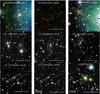 |
Fig. 1 Clusters discussed in this paper. We show pseudo-colour images for the cases where colour is available, using the MMT g′r′i′ bands. For the CL 1701+6414 field, we also show pseudo-colour images using the CFHT g′r′i′ bands, both for CL 1701+6414 and A 2246. We choose the ROSAT cluster coordinates as centre of the images. Note the variable background due to bright stars near CL 0159+0030 and CL 0809+2811. |
Definitions of the galaxy shape and lensing catalogues.
A detailed description of how we distill from a coadded image a galaxy shape catalogue, containing positions, ellipticity measurements, and photometric data for sources that can be considered galaxies can be found in Paper I. For the single-band clusters, we use straight-forward calls to SExtractor (Bertin & Arnouts 1996). For the three-band clusters, the convolution of images to the seeing in the poorest band and calls to SExtractor in double-detection mode, using the (unconvolved) r′-band image as the “detection image”, as described in Paper I are being performed.
We apply the “TS” shear measurement pipeline (Heymans
et al. 2006; Schrabback et al. 2007; Hartlap et al. 2009), an implementation of the KSB+
algorithm (Kaiser et al. 1995; Erben et al. 2001), which determines moments of the
brightness distribution for each source and corrects for the convolution with an
anisotropic PSF. The PSF anisotropy is traced by measuring the brightness distribution of
sources identified as stars in a plot of their magnitude
 against the
half-light radius ϑ. The values we used to define the boundaries of the
stellar locus are given in Table 2. Only sources in
the KSB catalogue, consisting of detections with a viable measurement of
ϑ, are further considered.
against the
half-light radius ϑ. The values we used to define the boundaries of the
stellar locus are given in Table 2. Only sources in
the KSB catalogue, consisting of detections with a viable measurement of
ϑ, are further considered.
Consistent with our Paper I findings, MMT/MegaCam exhibits a smooth, albeit variable pattern of PSF anisotropy which can be modelled by a low-order (2 ≤ dani ≤ 5, see Table 2) polynomial in image coordinates such that the residual PSF anisotropy has a practically vanishing mean value and a dispersion 0.005 ≤ σ(eani) ≤ 0.010 in the r′-band image stacks. In terms of the uncorrected PSF anisotropy, however, there are considerable differences in the input images for different cluster fields. Excessive PSF anisotropy observed in several input frames – which thus had to be removed from the coadded images – can be attributed to either tracking or focussing issues of the telescope. In most fields, no extreme outliers were present or could be easily identified. Only frames with average PSF ellipticity |⟨e ⟩|< 0.06 entered the coaddition. No clear distinction leaving a sufficient number of low-anisotropy frames was possible for the CL 1641+4001 and CL 1701+6414 fields. In these cases, all frames with |⟨e ⟩|< 0.10 were used for coaddition.
We classify as galaxies all sources fainter than the brightest unsaturated point sources
( ) and
more extended than the PSF (
) and
more extended than the PSF ( ). Because
even poorly resolved galaxies carry a lensing signal, we add sources
). Because
even poorly resolved galaxies carry a lensing signal, we add sources
 and
and  with
with
 to the
galaxy shape catalogue (cf. Fig. 4 of Paper I). The parameters defining this catalogue for
each field are tabulated in Table 2, together with
its number
density ngal ≈ nKSB/2.
to the
galaxy shape catalogue (cf. Fig. 4 of Paper I). The parameters defining this catalogue for
each field are tabulated in Table 2, together with
its number
density ngal ≈ nKSB/2.
2.4. Background selection
Cluster weak lensing studies rely on carefully selected catalogues of background galaxies, the carriers of the lensing signal. While falling short of yielding a reliable photometric redshift (photo-z) estimate for each individual galaxy, three-colour imaging makes possible a selection of foreground, cluster, and background sources based on their distribution in colour-colour–magnitude space (cf. Medezinski et al. 2010; Klein et al., in prep.). The method described below that we use for the three-band clusters is an improved version of the background selection in Paper I, to which we refer for concepts and terminology: While considering all galaxies fainter than mfaint in the lensing catalogue, galaxies brighter than mbright are rejected. In the intermediate regime (mbright < r′ < mfaint), we include galaxies whose g′ − r′ versus r′ − i′ colours are consistent with sitting in the background of the cluster, based on the – similarly deep – Ilbert et al. (2009) photo-z catalogue (see Appendix B for more details).
For the single-band clusters, the background selection simplifies to a magnitude cut,
meaning that lensing catalogue consists of all galaxies
r′ > mfaint.
For each of these sources, our KSB+ implementation yields a PSF-corrected ellipticity
ε = ε1 + iε2, a
noisy but, in principle, unbiased estimate of the reduced gravitational shear
g = g1 + ig2
(cf. Schneider 2006). We choose the values of
mfaint (and mbright where
applicable) such that the signal-to-noise ratio of the aperture mass estimator, or
S-statistics (Schneider 1996) is
optimised: 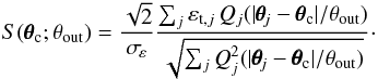 (1)By
εt,j = Re [εexp(−2iϕ)] ,
we denote the tangential ellipticity of the galaxy at position
(1)By
εt,j = Re [εexp(−2iϕ)] ,
we denote the tangential ellipticity of the galaxy at position
 , which with
respect to the point
, which with
respect to the point  has a phase
angle ϕ. Equation (1)
considers the noise from intrinsic source ellipticity, measured as
has a phase
angle ϕ. Equation (1)
considers the noise from intrinsic source ellipticity, measured as
 ;
while
Qj(| θθθj − θθθc|/θout)
is the Schirmer et al. (2007) filter function with
outer radius θout, maximising S for a
cluster-like radial shear profile.
;
while
Qj(| θθθj − θθθc|/θout)
is the Schirmer et al. (2007) filter function with
outer radius θout, maximising S for a
cluster-like radial shear profile.
We evaluate Eq. (1) on a regular grid with 15″ mesh size. With the notable exception of CL 1701+6414 (Sect. 4.1), the signal peaks are found close to the ROSAT-determined cluster centres and can be easily identified with our clusters. The adopted values of mbright, mfaint, and θout, yielding an optimal signal-to-noise ratio Smax are summarised in Table 2, as well as the number density nlc in the lensing catalogue3. We refer to the grid cell in which Smax occurs as the cluster shear peak and discuss the significance of our cluster detections in Sect. 7.1.
2.5. Shear profile modelling
Additional parameters defining the “default” cluster models.
Pursuing the approach adopted in Paper I, we model the tangential ellipticity profile
εt(θ) of our clusters with the reduced
shear profile
g(θ;r200,cNFW)
(Bartelmann 1996; Wright & Brainerd 2000) corresponding to the Navarro et al. (1995, 1996,
1997, NFW) density profile. From the estimate of
the radius r200 – defined such that the density of the
enclosed matter exceeds the critical density
ρc(zd) at the cluster redshift
zd by a factor of Δ = 200 – we infer the cluster mass
M200 via 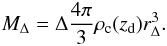 (2)The best matching
cluster mass profile parameters r200 and
cNFW minimise the merit function
(2)The best matching
cluster mass profile parameters r200 and
cNFW minimise the merit function 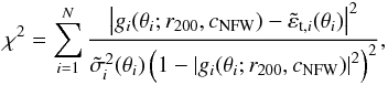 (3)which we evaluate on a
regular grid in r200 and cNFW. By
(3)which we evaluate on a
regular grid in r200 and cNFW. By
 ,
we denote the tangential component of the scaled
ellipticity
,
we denote the tangential component of the scaled
ellipticity  for the
ith galaxy, including a global shear calibration factor
f0 = 1.08 (see Paper I and Hartlap et al. 2009) as well as a separation-dependent correction
f1(θ) for the shear dilution by cluster
members (detailed below). Accordingly, the error scales as
for the
ith galaxy, including a global shear calibration factor
f0 = 1.08 (see Paper I and Hartlap et al. 2009) as well as a separation-dependent correction
f1(θ) for the shear dilution by cluster
members (detailed below). Accordingly, the error scales as
 with σε from Sect. 2.4. The index i runs over all lensing catalogue
galaxies with separations within the fitting range
θmin ≤ θ ≤ θmax
from the assumed ROSAT cluster centre, presented in Table 3. We choose separations θmin and
θmax corresponding to distances of
rmin = 0.2 Mpc and
rmax = 5.0 Mpc at the respective cluster redshift. The
denominator of Eq. (3) accounts for the
dependence of the noise on
gi(θi)
itself (Schneider et al. 2000).
with σε from Sect. 2.4. The index i runs over all lensing catalogue
galaxies with separations within the fitting range
θmin ≤ θ ≤ θmax
from the assumed ROSAT cluster centre, presented in Table 3. We choose separations θmin and
θmax corresponding to distances of
rmin = 0.2 Mpc and
rmax = 5.0 Mpc at the respective cluster redshift. The
denominator of Eq. (3) accounts for the
dependence of the noise on
gi(θi)
itself (Schneider et al. 2000).
Source redshift distributions.
The reduced shear gi(θi) exerted by a lens on the image of a background source further depends on the ratio of angular diameter distances between deflector and source Dds and source and observer Ds. For each of our fields, we estimate a catalogue-average ⟨β⟩ = ⟨Dds/Ds⟩i = 1...N using the Ilbert et al. (2006) photo-z catalogue, drawn from the CFHTLS Deep fields with similar source number counts as a function of magnitude r′ as our MMT observations. Applying the same photometric cuts as to the MMT data to the catalogues of reliable photo-z sources (cf. Paper I), we thus obtain proxy redshift distributions for our cluster observations. We repeat the fit of a van Waerbeke et al. (2001) redshift distribution and subsequent calculation of ⟨β⟩ as described in Paper I – but to an improved accuracy – for all combinations of MMT and CFHT Deep fields. As an input to Eq. (3), we use the mean ⟨⟨β⟩⟩k = 1...4 (Table 3) measured for the Deep fields and consider its dispersion σ(⟨ β⟩) in the error analysis (Sect. 6.1).
We further employ the Ilbert et al. (2006)
catalogue to test the efficacy of the background selection. Applying the respective
background selection to the Deep 1 photo-z catalogue, we determine the
fraction  of residual foreground galaxies in the lensing catalogues (Table 3, cf. Sect. 6.1).
Dilution by cluster members.
Although the selection of lensing catalogue galaxies is designed to include preferentially background galaxies, we detect an increase in the fraction frsc(θ) of galaxies whose g′ − i′ colours are consistent with the red sequences at zd towards the centres of our three-band clusters. Tentative red sequence galaxies are defined using an interval in g′ − i′ empirically found in the g′ − i′ versus i′ colour–magnitude diagram, around the expected colour of a Coleman et al. (1980) early-type galaxy calculated with the Bolzonella et al. (2000) photo-z code. To correct for the dilution effect of these likely unlensed sources in the shear catalogues, the corrective factor f1(θ) = 1 + Σ(θ)/ [Σ(θ) + B] is introduced. The NFW surface mass profile Σ(θ) and background term B are determined by a fit to frsc(θ). We apply this correction only to the three-band clusters for which the g′ − i′ information is available (see Table 3). Because we have f1(θ) measured for only four clusters, three of which suffer from large masks in the crucial central regions, we decide against using an averaged f1(θ) for the single-band clusters at this stage of the survey.
2.6. Surface mass maps
While we use the tangential shear profile to determine cluster masses, we are interested as well in the (projected) mass distributions of our clusters in order to distinguish possibly merging systems of disturbed morphology from relaxed clusters. The non-local relation between shear and convergence κ = Σ/Σcrit can be inverted, as shown by Kaiser & Squires (1993). We perform mass reconstructions using the Seitz & Schneider (1996, 2001) finite-field inversion algorithm. Concerning the mass sheet degeneracy (cf. Schneider 2006), the mean κ along the edge of the field-of-view is assumed to vanish.
The dimensionless surface mass  , with an arbitrary normalisation,
is calculated on a regular grid. Because each cluster field has to be divided into an
integral number of grid cells, the mesh size cannot be fixed to the same constant for all
clusters, but varies slightly, with a mean of
, with an arbitrary normalisation,
is calculated on a regular grid. Because each cluster field has to be divided into an
integral number of grid cells, the mesh size cannot be fixed to the same constant for all
clusters, but varies slightly, with a mean of  and a standard deviation of
 . For all clusters and grid
points, the algorithm accounts for lensing catalogue galaxies within a radius of
θs = 2′. The input shear field is smoothed with a truncated
Gaussian filter of 0.555 θs full-width half-maximum, which
drops to zero at θs.
. For all clusters and grid
points, the algorithm accounts for lensing catalogue galaxies within a radius of
θs = 2′. The input shear field is smoothed with a truncated
Gaussian filter of 0.555 θs full-width half-maximum, which
drops to zero at θs.
3. Results for normal clusters
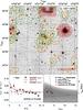 |
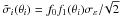
Fig. 2 Lensing results for CL 1357+6232. Upper panel: MegaCam
r′-band image (cut-out of ~20′ side length), overlaid
with S-statistics (orange solid) and
|


In this Section, we present the outcome of the WL modelling, by showing a comprehensive figure combining the lensing signal maps, shear profile, and NFW modelling for each cluster. CL 1357+6232 (Fig. 2) serves as our example; for more details on the other clusters, we refer to Figs. D.1 to Figs. D.4 in Appendix D. Two clusters, CL 1701+6414 (Fig. 3) and CL 1641+4001 (Fig. 5), exhibit multiple shear peaks and shear profiles that are very flat but positive over a large radial range. The more involved modelling of these “special cases” – as opposed to the “normal clusters” – is described in Sect. 4.
In the upper panel of Fig. 2, we present the
S-statistics (solid orange) and  -contours
(green dashed) for CL 1357+6232, overlaid on a cut-out of the MegaCam
r′-band image with ~20′ side length. Masked areas can be
identified from the red polygons (mostly squares). The ROSAT centre is given by a yellow,
eight-pointed star symbol. A filled orange square denotes the shear peak grid cell
(Sect. 2.4), while a star symbol with error bars
shows the WL centre from bootstrapping (Sect. 3.2).
-contours
(green dashed) for CL 1357+6232, overlaid on a cut-out of the MegaCam
r′-band image with ~20′ side length. Masked areas can be
identified from the red polygons (mostly squares). The ROSAT centre is given by a yellow,
eight-pointed star symbol. A filled orange square denotes the shear peak grid cell
(Sect. 2.4), while a star symbol with error bars
shows the WL centre from bootstrapping (Sect. 3.2).
The lower left panel of Fig. 2 shows the binned shear profile ⟨εt(θ)⟩ as filled circles with error bars giving the dispersion of the measured values. Open diamonds give the cross component ⟨ε × (θ)⟩ which is on average expected to be consistent with zero for cluster lenses. The red solid line denotes the best-fit NFW model. Finally, the lower right panel of Fig. 2 presents Δχ2(r200,cNFW) = χ2 − min(χ2). The minimum is indicated by filled circle; contour lines enclose the 99.73%, 95.4%, and 68.3% confidence regions, (i.e. Δχ2 = 2.30, 6.17, and 11.30). An upward triangle marks the minimum of Δχ2 when restricting cNFW to its Bullock et al. (2001, dashed line) value.
3.1. Cluster detection and lensing morphology
We successfully detect all observed 400d clusters using the S-statistics
with at least 3.5σ significance and are able to derive a weak lensing
mass estimate for each cluster. Table 2 summarises
the maximum detection levels S and the optimal filter scales
 . The most
significant detection is CL 0030+2618 at z = 0.50 with
S = 5.84 (Paper I); the formally least significant detection is
CL 0230+1836 at z = 0.80 with S = 3.64.
The S = 3.75 measured for CL 1701+6414 has a contribution from the
nearby cluster A 2246 at θ ≈ 270″ separation (Sect. 4.1), rendering it the least secure detection: for
θout = 220″, we detect CL 1701+6414 at the
2.5σ level. By detecting CL 0230 +1836, we demonstrate the feasibility
of MegaCam WL studies out to the highest redshifts accessible for current ground-based
weak lensing.
. The most
significant detection is CL 0030+2618 at z = 0.50 with
S = 5.84 (Paper I); the formally least significant detection is
CL 0230+1836 at z = 0.80 with S = 3.64.
The S = 3.75 measured for CL 1701+6414 has a contribution from the
nearby cluster A 2246 at θ ≈ 270″ separation (Sect. 4.1), rendering it the least secure detection: for
θout = 220″, we detect CL 1701+6414 at the
2.5σ level. By detecting CL 0230 +1836, we demonstrate the feasibility
of MegaCam WL studies out to the highest redshifts accessible for current ground-based
weak lensing.
In general, we find a very good agreement between the signal morphologies, of the S-statistics and mass reconstruction, i.e. we detect the same structures at comparable relative signal strength. This result reaffirms that our detections are not caused by artifacts in the (independent) analysis methods.
3.2. WL cluster centres
We define a “default” model for the NFW modelling of each cluster, determined by the parameters in Table 3, i.e. the cluster centre, fitting range, ⟨⟨β⟩⟩, and dilution correction. We acknowledge that a careful and consistent treatment of cluster centres is important to prevent masses from being biased. In the default model, we use the lensing-independent ROSAT X-cluster centres. For comparison, we also consider cluster centres based on the S-map, which provide us with a high signal-to-noise shear profile. The shear peaks (most significant cell in the S-map) are thoroughly studied with respect to the background selection parameters and their interpretation as significances (Sect. 7.1).
The S-peak of CL 0159+0030 is located conspicuously close to the edge of an extended shear plateau which is likely caused by a large masked area4 around a bright star (V = 8.3, Figs. 1 and D.1). Similarly bright stars are present also close to CL 0230+1836 and CL 0809+2811 (Figs. D.2 and D.3). In the latter case, where the S-peak lies within the masked area, we discuss the effect of masking in Sect. 7.5.
As noise can boost S in a grid cell compared to its neighbours, we perform a bootstrap resampling of the S-map (cf. Paper I) in two cases, CL 1357+6232 and CL 1416+4446. Averaging over 105 realisations, for which we draw Nlc galaxies with repetitions from the lensing catalogue, we determine a lensing centre. We find the bootstrap lensing centres to be in good agreement with the shear peaks of CL 1357+6232 and CL 1416+4446, well within the standard deviation of the bootstrap samples. In Sect. 7.2, the implications of the choice of cluster centres for the mass estimates are discussed.
3.3. Shear profiles and NFW modelling
Five of our clusters can be classified as “normal”, characterised by centrally increasing ⟨εt⟩(θ) profiles, in good agreement with the NFW models. As expected, their ⟨ε × ⟩(θ) profiles are consistent with zero, with fluctuations that can be explained by shape noise. The two other clusters, CL 1641+4001 and CL 1701+6414 show a more complicated morphology in their S-maps (Sect. 4).
Table 4 provides the cluster parameters resulting
from the NFW modelling. Uncertainties in r200 and
cNFW are calculated from Δχ2
corresponding to a 68.3% confidence limit for one interesting parameter
(Δχ2 = 1). Cluster masses
 are inferred via Eq. (2).
3.4. Mass-concentration relations
Weak lensing hardly constrains cluster concentration parameters, because the dependence on cNFW is highest in the cluster centre where few lensed sources are observed. This is reflected also in our results, with huge uncertainties measured for cNFW in several objects. Hence, we perform two additional measurements, in which we fix the value of cNFW.
The first mass-concentration relation we assume is the one found by Bullock et al. (2001, B01) for simulated clusters: 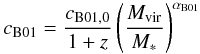 (4)with
cB01,0 = 9.0,
αB01 = −0.13, and
M ∗ = 1.3 × 10¹³ h-1 M⊙.
In their simulations, B01 observe a scatter of
σ(log cvir) = 0.18 for a fixed
Mvir.
(4)with
cB01,0 = 9.0,
αB01 = −0.13, and
M ∗ = 1.3 × 10¹³ h-1 M⊙.
In their simulations, B01 observe a scatter of
σ(log cvir) = 0.18 for a fixed
Mvir.
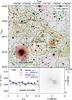 |
Fig. 3 Shear signal in the CL 1701+6414 field and its best-fit model with two NFW components accounting for CL 1701+6414 and A 2246. Upper plot: the layout follows Fig. 2. The ROSAT position of A 2246 is marked by a big four-pointed star symbol. Smaller star symbols denote positions of further X-ray clusters. Lower left plot: the layout follows Fig. 2. The solid blue and dashed red lines give the mean tangential and cross shear components, averaged in bins around the CL 1701+6414 shear peak, as expected from the two-cluster model. The separation of the two main clusters is indicated by a vertical dotted line. Lower right plot: the orientations and amplitudes of the shear, as expected from the best-fit two-cluster model, calculated on a regular grid. |
Synopsis of cluster parameters and resulting weak lensing masses.
For our purposes, we insert for
Mvir in Eq. (4). Due to the weak dependence of cB01 on
Mvir this results only in a very small underestimate of
cB01. For two of the total of eight clusters we analysed,
cB01 is very close to the cNFW
obtained by lensing, while for others it differs strongly (see Table 4).
Assuming the B01 mass-concentration relation, we apply a Gaussian prior
pc(r200,c200)
with standard deviation σ(log c200) = 0.18 to
the tabulated values of Δχ2(r200,
cNFW) for each of our clusters, and marginalise over
the c200 dimension. The radii
r200,B01 and the corresponding masses
 , found from the minimum of
∑ jpc(r200,c200,j)
Δχ2(r200,c200,j)
are listed in Table 4.
, found from the minimum of
∑ jpc(r200,c200,j)
Δχ2(r200,c200,j)
are listed in Table 4.
We notice that the simulations from which the B01 relation was measured assume
σ8 = 1.0 to fix the normalisation of the matter power
spectrum. This value is inconsistent with more recent measurements of cosmological
parameters (e.g. Larson et al. 2011; Burenin & Vikhlinin 2012). Hence, we consider a
second mass-concentration relation, based on a recent suite of simulations employing
σ8 = 0.8 as favoured by currents models: Bhattacharya et al. (2011, B12) study dark matter haloes
of massive clusters and find that the concentration parameter can be modelled with a
single power law when expressed in terms of the peak height parameter ν
from linear collapse theory5. Their simulated
clusters are best represented by: 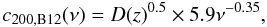 (5)with a variance of
σc = 0.33c200. We compute the
growth factor D(z) for a flat Universe with a
cosmological constant. In complete analogy to the B01 relation, we compute cluster
radii r200,B12 and
masses
(5)with a variance of
σc = 0.33c200. We compute the
growth factor D(z) for a flat Universe with a
cosmological constant. In complete analogy to the B01 relation, we compute cluster
radii r200,B12 and
masses  for each cluster, given
the c200-M200–relation resulting
from Eq. (5). The results are presented in
Table 4.
for each cluster, given
the c200-M200–relation resulting
from Eq. (5). The results are presented in
Table 4.
4. Special cases
4.1. CL 1701+6414
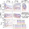 |
Fig. 4 Simultaneous NFW modelling of CL 1701+6414 and A 2246. Each panel shows the
dependencies between two of the four parameters, with the other two marginalised.
Solid confidence contours (1σ, 2σ,
3σ) denote the default case, using the ROSAT centres; dashed
contours denote models centred on the S-peaks. The respective
parameters minimising |
4.1.1. X-ray clusters and shear peaks
A weak lensing analysis of CL 1701+6414 has to deal with shear by multiple structures.
The strongest shear peak (S = 4.3σ) in Fig. 3 coincides with the most prominent cluster in the
field amongst optical galaxies6, Abell 2246 (big
four-pointed star symbol in Fig. 3),
 to the west of CL 1701+6414.
With a redshift of z = 0.225 (Vikhlinin
et al. 1998; Burenin et al. 2007),
A 2246 is part of the 400d parent sample, but not of the distant cosmological sample.
CL 1701+6414, for whose detection in the S-statistics the lensing
catalogue was optimised, is detected at the 3.7σ level. The ROSAT
catalogue of Vikhlinin et al. (1998) lists two
further clusters in the field, VMF 191 at z = 0.220 and VMF 192 at
z = 0.224 (small star symbols in Fig. 3), which we identify with S-peaks of 2.9σ
and 2.7σ, respectively. Another 3.1σ peak lies
close-by. A zone of positive shear signal extends over >20′,
from the north-east of VMF 192 to a 3.6σ shear peak south-west of
A 2246, which does not correspond to a known cluster. Noticing the very similar
redshifts of A 2246, VMF 191, and VMF 192, we likely are observing a physical filament
at z = 0.22, through whose centre we see CL 1701+6414 in projection.
Luckily, a likely strong lensing arc, 10″ to the west of the BCG of CL 1701+6414
(z = 0.44 ± 0.01, Reimers et al.
1997) gives direct evidence that CL 1701+6414 acts as a gravitational lens. We
find no significant WL signal near the ROSAT source RX J1702+6407 (Donahue et al. 2002, cf. Appendix D.6).
to the west of CL 1701+6414.
With a redshift of z = 0.225 (Vikhlinin
et al. 1998; Burenin et al. 2007),
A 2246 is part of the 400d parent sample, but not of the distant cosmological sample.
CL 1701+6414, for whose detection in the S-statistics the lensing
catalogue was optimised, is detected at the 3.7σ level. The ROSAT
catalogue of Vikhlinin et al. (1998) lists two
further clusters in the field, VMF 191 at z = 0.220 and VMF 192 at
z = 0.224 (small star symbols in Fig. 3), which we identify with S-peaks of 2.9σ
and 2.7σ, respectively. Another 3.1σ peak lies
close-by. A zone of positive shear signal extends over >20′,
from the north-east of VMF 192 to a 3.6σ shear peak south-west of
A 2246, which does not correspond to a known cluster. Noticing the very similar
redshifts of A 2246, VMF 191, and VMF 192, we likely are observing a physical filament
at z = 0.22, through whose centre we see CL 1701+6414 in projection.
Luckily, a likely strong lensing arc, 10″ to the west of the BCG of CL 1701+6414
(z = 0.44 ± 0.01, Reimers et al.
1997) gives direct evidence that CL 1701+6414 acts as a gravitational lens. We
find no significant WL signal near the ROSAT source RX J1702+6407 (Donahue et al. 2002, cf. Appendix D.6).
4.1.2. Two-cluster modelling of MMT data
Plotting the binned tangential shear around the lensing centre (lower left panel of Fig. 3), we find a flat profile whose average ⟨εt(θ)⟩ > 0 is consistent with the extended shear signal in the S-map. The cross-component ⟨ε × (θ)⟩ is consistent with zero. Acknowledging the prominent signal related to A 2246, we model the shear of CL 1701+6414 and A 2246, simultaneously, using an NFW shear profile for each deflector.
We assume both the shear gp of the primary and
gs of the secondary component to be small. In this limit,
the shear components originating from both lenses become additive:
 (6)with
α = 1,2. Here,
rp,200,
rs,200,
cp,NFW, and
cs,NFW are the radii and concentration
parameters of the primary and secondary component. Note that
gadd,α(θθθ)
explicitly depends on the two-dimensional coordinate vector
(6)with
α = 1,2. Here,
rp,200,
rs,200,
cp,NFW, and
cs,NFW are the radii and concentration
parameters of the primary and secondary component. Note that
gadd,α(θθθ)
explicitly depends on the two-dimensional coordinate vector
 :
the shear field of two clusters no longer has radial, but only axial symmetry. This is
illustrated in the lower right panel of Fig. 3,
showing the shear fit expected from the best-fit two-cluster model for the CL 1701+6414
lensing catalogue, evaluated on a regular grid. We consider a modification of the merit
function given by Eq. (3):
:
the shear field of two clusters no longer has radial, but only axial symmetry. This is
illustrated in the lower right panel of Fig. 3,
showing the shear fit expected from the best-fit two-cluster model for the CL 1701+6414
lensing catalogue, evaluated on a regular grid. We consider a modification of the merit
function given by Eq. (3): 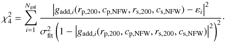 (7)The symbol
 highlights
the dependence on four parameters, the radii and concentrations of the two clusters.
Note that models the
measured εi directly, without recourse to a
definition of the tangential component.
highlights
the dependence on four parameters, the radii and concentrations of the two clusters.
Note that models the
measured εi directly, without recourse to a
definition of the tangential component.
We assumed ⟨⟨β⟩⟩ = 0.381 for CL 1701+6414 (Table 3) and ⟨⟨β⟩⟩ = 0.640 for A 2246, calculated the same way as for the other clusters. The average tangential and cross-component of the shear expected in concentric annuli around the centre of CL 1701+6414 are presented in the lower left panel of Fig. 3. A vertical dotted line denotes the separation of CL 1701+6414 and A 2246. We find a good agreement to the measured shear and note that due to the lack of radial symmetry the dispersion of the model values in the annuli is of the same order as the measurement errors. Although the cross-component can be large at some points in the image plane, ⟨g × ⟩ cancels out nearly completely when averaging over the annuli.
Figure 4 presents the confidence contours and parameters minimising Eq. (7) for the default model (filled circle and solid contours). The panels of Fig. 4 show all combinations of two fit parameters, where we marginalised over the two remaining ones. Owing to the 4-dimensional parameter space, we tested a coarse grid of points to avoid excessive computing time. The picture emerges that rp,200 and rs,200 are relatively independent of each other (top right panel). Hence, the presence of the respective other cluster does not seem to affect the accuracy with which we can determine the masses of the two clusters strongly. The data favour the smallest tested value, cp,NFW = 0.5 for the concentration of CL 1701+6414, and the largest one, cs,NFW = 15.5, for A 2246. Using shear peak cluster centres (dashed contours and upward pointing triangle in Fig. 4), cp,NFW is also very low, but the uncertainties are large. The poor constraint on cs,NFW might be partly due to the masking of the centre of A 2246 or shear contribution by the BCG.
Given the absence of a strong covariance between the parameters of A 2264 and
CL 1701+6414, we fix the parameters of the foreground cluster to
rs,200 = 0.90 Mpc and
cs,NFW = 20 and repeat the analysis with
our usual, finer parameter grid. The best model is found for
 ,
confirming the results from Fig. 4. We note that we
find a low cp,NFW, although our model
explicitly accounts for the extra shear by A 2246. Using the default model, we compute
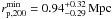
masses of
,
confirming the results from Fig. 4. We note that we
find a low cp,NFW, although our model
explicitly accounts for the extra shear by A 2246. Using the default model, we compute
masses of  for
CL 1701+6414 and
for
CL 1701+6414 and  for A 2246,
based on
for A 2246,
based on  .
.
4.1.3. Comparison to CFHT data
In addition, Fig. 4 shows confidence contours obtained from a WL analysis of CFHT observations of the CL 1701+6414 field (r′-band, ≈ 7200 s), which we discuss in greater detail in Sect. 5. We repeated the two-cluster modelling using Eq. (7) following the same data reduction and shear measurement pipelines. Besides mfaint = 20.2 and the PSF-dependent galaxy selection, parameters are kept at their MMT values.
The resulting cluster parameters minimising  (red
downward triangles for ROSAT and diamonds for S-peak centres) and the
corresponding thin confidence contours in Fig. 4
show agreement with the MMT data within the 2σ margins or better.
With
(red
downward triangles for ROSAT and diamonds for S-peak centres) and the
corresponding thin confidence contours in Fig. 4
show agreement with the MMT data within the 2σ margins or better.
With  ,
and
,
and  ,
relating to WL masses of
,
relating to WL masses of  for
CL 1701+6414 and
for
CL 1701+6414 and  for A 2246, we
arrive at lower masses, especially for CL 1701+6414, but consistent within the
uncertainties of the MMT data. Using the S-peaks as centres yields very
similar results.
for A 2246, we
arrive at lower masses, especially for CL 1701+6414, but consistent within the
uncertainties of the MMT data. Using the S-peaks as centres yields very
similar results.
Our CFHT data give more plausible best-fit concentration parameters of
 for
A 2246, and
for
A 2246, and  for
CL 1701+6414, although the constraints are poor. We conclude that a dual-NFW modelling
is feasible, but more sensitive to the choice of cluster centres than a single NFW fit
to r200 and cNFW. Adding more
cluster components would even increase these interdependencies. However, the main point
here is that the MMT and CFHT analyses agree.
for
CL 1701+6414, although the constraints are poor. We conclude that a dual-NFW modelling
is feasible, but more sensitive to the choice of cluster centres than a single NFW fit
to r200 and cNFW. Adding more
cluster components would even increase these interdependencies. However, the main point
here is that the MMT and CFHT analyses agree.
4.2. CL 1641+4001
The S-statistics map of CL 1641+4001 exhibits several shear peaks which form a connected structure of >20′ extent (Fig. 5). Located within a plateau of S > 3σ significance, the ROSAT centre of CL 1641+4001 (big star symbol) is separated by 95″ from the primary (S = 4.12) shear peak and by 125″ from the secondary (S = 3.95, orange triangle in Fig. 5) shear peak. The BCG of CL 1641+4001 can be found between the ROSAT centre and primary shear peak.
The ⟨εt(θ)⟩ profile (lower left panel of
Fig. 5) centred on the main shear peak profile is
flat, with a positive average in all bins and the most significant positive signal at
~9′ distance from the cluster centre. In the innermost two bins
( ),
⟨ε × (θ)⟩ is of similar amplitude as
the tangential component, but consistent with zero at the 1σ level.
Similar to CL 1701+6414, the modelling using Eq. (3) finds a very low
),
⟨ε × (θ)⟩ is of similar amplitude as
the tangential component, but consistent with zero at the 1σ level.
Similar to CL 1701+6414, the modelling using Eq. (3) finds a very low  ,
consistent with zero and reflecting the flat shear profile.
,
consistent with zero and reflecting the flat shear profile.
The only cluster candidate in the literature besides CL 1641+4001 is SDSS-C4-DR3 3628 at z = 0.032, identified in the SDSS Data Release 3, using the Miller et al. (2005) algorithm, but published solely by von der Linden et al. (2007). We test a two-cluster model, introducing a second component at the redshift of SDSS-C4-DR3 3628, implying ⟨⟨β⟩⟩ = 0.940. We choose the second-highest shear peak as the centre of the secondary component. The offset of ~3′ to the coordinates of SDSS- C4-DR3 3628 (small star symbol in Fig. 5) is justified by the large mask at the latter position. The two-cluster fit yields a mass of order 1014 M⊙ for both the primary and the secondary component. This estimate is in stark disagreement with the absence of a massive, nearby cluster from our MMT image, which would have had to be missed by all but one cluster surveys.
At the same coordinates as SDSS-C4-DR3 3628 and also at z = 0.032, NED lists CGCG 224−092, a galaxy pair, dominated by the bright elliptical UGC 10512. These two galaxies are what we see in the MegaCam image7 and also in the SDSS image of the area. Inspection of the respective Chandra image shows significant X-ray emission, whose extent of ~30″ in diameter (~20 kpc at z = 0.032) is consistent with being caused by a massive elliptical galaxy or small galaxy group. With ≈1.7 × 1041 erg s-1 in the 2–10 keV range, its flux is high for a single galaxy, but the low temperature of ≈0.6 keV (obtained by fitting an absorbed APEC model) speaks against a galaxy group. In conclusion, we deem it unlikely that the complex structure in the S-map of CL 1641+4001 bears a significant contribution from the z = 0.032 structure.
We prefer the hypothesis that the shear is caused by a complex structure at the redshift
of CL 1641+4001, although its X-ray morphology does not hint at a merger (Vikhlinin et al. 2009a). Despite its shortcomings, we
return to the simplest explanation for the time being and model CL 1641+4001 by a single
NFW component: we obtain a minimum of χ2
for  and
and  .
These results, entailing a mass estimate of
.
These results, entailing a mass estimate of  are illustrated
by the filled circle and solid contours in the lower right panel of Fig. 5. Interestingly, choosing the secondary shear peak as a
centre yields similar cluster parameters to those found by choosing the primary shear
peak. This could hint at a major merger of similarly massive substructures, but more
observations are needed to test this hypothesis.
are illustrated
by the filled circle and solid contours in the lower right panel of Fig. 5. Interestingly, choosing the secondary shear peak as a
centre yields similar cluster parameters to those found by choosing the primary shear
peak. This could hint at a major merger of similarly massive substructures, but more
observations are needed to test this hypothesis.
5. Verification with independent data
5.1. CFHT observations
Observation dates, final exposure times and seeing values in the coadded CFHT/MegaCam data for CL 1701+6414.
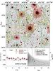 |
Fig. 5 Same as Fig. 2, but for CL 1641+4001. In the map, a triangle denotes the secondary shear peak, while a small star symbol marks the position of the von der Linden et al. (2007) cluster candidate. Note that no peak in the complex pattern of shear peaks correlates with its position. |
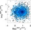 |
Fig. 6 Sample density of the ratio εMMT/εCFHT of the complex ellipticities measured for the matched galaxies from the MMT and CFHT r′-band catalogues, respectively. The shaded contours correspond to the logarithmic densities of all galaxies from the MMT lensing catalogue which have a match in the CFHT catalogue. Solid contours give the density of galaxies detected with a signal/noise ratio of ν > 15, the top 32.6%. Note that the normalisation of the ν > 15 galaxies is scaled up by 1/0.326 to obtain the same logarithmic contour levels. A Gaussian smoothing kernel of full-width half-maximum 0.075 was applied to both contour maps. |
CL 1701+6414 is the only cluster we observed with MMT/MegaCam for which deep, lensing-quality data obtained with another telescope exist. It has been observed in the g′r′i′z′ filters (P.I.: G. Soucail, Run ID: 2006AF26) using the MegaPrime/MegaCam at the Canada-France-Hawaii Telescope (CFHT)8. Table 5 lists the specifications of the CFHT data set. The CFHT data are processed with THELI in the same way as the MMT data, with a few CFHT-specific modifications to the code (cf. Erben et al. 2009), making use of the pre-processing available for archival CFHT data. Hence, the results are a suite of coadded and calibrated images in the g′r′i′z′ passbands, centred on CL 1701+6414, and with a side length of ~1° each. From the g′r′i′ images, we derived the pseudo-colour images of the centres of CL 1701+6414 and A 2246 in Fig. 1.
We employ the CFHT data for two kinds of consistency checks with the MMT data: First, we run the lensing pipeline on the deep CFHT r′ band image, applying the same shape recovery technique to the same objects, but observed with different instruments. The results of this comparison are detailed in Sect. 5.2. Second, making use of the CFHT imaging in four bands, we produced a BPZ (Benítez 2000) photometric redshift catalogue (Sect. 5.4 and Appendix C) with the goal of testing the single-band (magnitude cut) background selection in the CL 1701+6414 MMT lensing catalogue.
5.2. Comparative shape analysis
In this Subsection, we compare shape measurements obtained in the same field (the one of CL 1701+6414) using the MMT/MegaCam and CFHT/MegaCam instruments (cf. Sect. 5.1). Using the same parameter settings for our KSB pipeline, we extracted a KSB catalogue from the CFHT r′-band image. Subsequently, the CFHT and MMT catalogues were matched, using the associate and make_ssc tools available in THELI. With the smaller field-of-view of MMT/MegaCam defining the location of possible matches, 68.2% of sources in the MMT KSB catalogue are matched to a CFHT detection. Larger masked areas in the CFHT image – in particular due to reflections (so-called ghosts) around very bright stars – are the main cause impeding a higher matching fraction. Inside the MMT area (measuring at a safe distance from its low-weight edges), we find 85.5% of the CFHT sources to be detected by MMT.
We note that objects in the matched catalogue have comparable SExtractor signal-to-noise ratios ν in both r′-band images. Considering objects with νMMT > 15 – the top quartile of all objects in the catalogue of matches – for which selection effects should be negligible, we measure ⟨νCFHT/νMMT⟩ = 0.832, with a dispersion of 0.057. These values show little dependence on the limiting value of νMMT, and confirm the visual impression that the r′-band images are of similar depth9.
With these preparatory analyses in mind, we investigate the relation between the ellipticities observed with CFHT and MMT. Figure 6 presents the ratio εMMT/εCFHT of the complex ellipticities measured by KSB on the MMT and CFHT images10. Shaded contours in Fig. 6 mark lines of equal density of the distribution of εMMT/εCFHT, as measured from the sources passing the criteria for the MMT galaxy catalogue (cf. Sect. 2.4). Using a grid of mesh size as small as 0.01 for both the real and imaginary axes, we find the density distribution of εMMT/εCFHT to scatter around its peak at unity. Note that the logarithmic scaling in Fig. 6 emphasises the wings of the distribution. When repeating the analysis restricted to galaxies detected with νMMT > 15 – the top 32.6% of the matched sources contained in the MMT galaxy catalogue – the peak at εMMT = εCFHT persists, while the scatter is slightly reduced (solid contours in Fig. 6). This can be seen comparing the two outermost solid contours to the shaded contours, indicating the same levels of number density.
This means, any systematic bias between shear measurements obtained with MMT and CFHT is smaller than a few percent. We expect a small bias, below the sensitivity of our measurement, to be present because of the dependence of the shear calibration factor f0 on magnitude and half-light radius ϑ (cf. Appendix C of Hartlap et al. 2009). In addition to our results from Paper I, the consistent galaxy ellipticities measured with MMT and the well-established CFHT/MegaCam mark further evidence that MMT/MegaCam is well-suited for measuring weak gravitational lensing signals.
5.3. S-statistics from CFHT and MMT
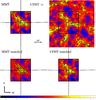 |
Fig. 7 S-statistics in the CL 1701+6414 field drawn from the MMT
(top left), CFHT (top right), and matched
sources catalogues (bottom panels). The linear colour scale,
contours indicating levels of S = 1 to S = 4,
|
Figure 7 provides a qualitative comparison of the
S-maps for CL 1701+6414 obtained with both CFHT and MMT. Its upper two
panels show the independent shear catalogues drawn from the r′
images of both instruments, at the respective optimal values
 and
and
 for
for
 . The distribution of the
S-signal in the overlapping region inside the MMT field-of-view (black
square in Fig. 7) is astonishingly similar: not only
do we find the tentative filament from the north-east of VMF 192 to the south-west of
A 2246 (compare Fig. 3 and the black lines in
Fig. 7 indicating
the αJ2000 and δJ2000 of
CL 1701+6414). Moreover, also the regions of high S at the eastern and
north-western edges of the MMT field-of-view correspond to peaks in the CFHT
S-map. Whereas the detection significance at the peak closest to the
position of CL 1701+6414 is smaller for CFHT (S = 2.89 compared to
S = 3.75), it is also more prominent in the sense of a deeper “valley”
separating it from the dominant A 2246 peak (S = 4.30 in both the MMT and
CFHT maps).
. The distribution of the
S-signal in the overlapping region inside the MMT field-of-view (black
square in Fig. 7) is astonishingly similar: not only
do we find the tentative filament from the north-east of VMF 192 to the south-west of
A 2246 (compare Fig. 3 and the black lines in
Fig. 7 indicating
the αJ2000 and δJ2000 of
CL 1701+6414). Moreover, also the regions of high S at the eastern and
north-western edges of the MMT field-of-view correspond to peaks in the CFHT
S-map. Whereas the detection significance at the peak closest to the
position of CL 1701+6414 is smaller for CFHT (S = 2.89 compared to
S = 3.75), it is also more prominent in the sense of a deeper “valley”
separating it from the dominant A 2246 peak (S = 4.30 in both the MMT and
CFHT maps).
The second-most significant (4.08σ) shear peak in the CFHT S-map is at αJ2000 = 17h01m57s, δJ2000 = +63°51′, outside the southern edge of the MMT field-of-view, with no known cluster but several brighter (r′ < 20) galaxies in the vicinity.
Can the subtle differences between the MMT and CFHT S-maps be attributed to shape noise or rather to selection of galaxies at the faint end? We investigate that by considering the matched-sources catalogue from Sect. 5.2 and apply to it the combined selection criteria for the MMT and CFHT lensing catalogues (e.g. both |εMMT| < 0.8 and |εCFHT| < 0.8). The resulting S-maps derived from the MMT and CFHT ellipticities of the exact same sources are displayed in the lower left and lower right panels of Fig. 7. Naturally, all matched sources are located within the MMT field-of-view. Qualitatively, the matched S-maps again show the same structure, although they do not appear to be much more similar than the S-maps drawn from the individual catalogues. This indicates that galaxy selection plays a relevant role. We note that based on the CFHT shapes of the matched galaxies, CL 1701+6414 is the most significant detection with S = 3.46, while the A 2246 peak is suppressed by ≈1σ compared to the pure CFHT map.
Quantitatively, the Pearson correlation coefficient of ϱ = 0.912 between
the matched-sources S maps substantiates the visual impression of a high
correlation. When the faintest ≈20% of galaxies are removed from the matched catalogue,
considering only galaxies brighter than  in
both the MMT and CFHT images, this value increases to ϱ = 0.926. Removing
the faintest ≈40% of galaxies by imposing
in
both the MMT and CFHT images, this value increases to ϱ = 0.926. Removing
the faintest ≈40% of galaxies by imposing  , it
further rises to ϱ = 0.938.
, it
further rises to ϱ = 0.938.
The detection of the same shear peaks reassures us that the multi-peaked S-distribution analysed in detail in Sect. 4.1 traces an actual shear signal and removes any doubts that the S-filament across the MMT field-of-view could be merely an instrument-dependent artefact, e.g. residuals of improper PSF anisotropy correction.
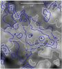 |
Fig. 8 Average and difference aperture mass ℳ ± (Eq. (8)), measured in the matched MMT-CFHT catalogue. The grey-scale and white contours give ℳ−, the thicker blue contours show ℳ+. The spacing for both contours is in multiples of 0.015, starting at 0. Black circles mark the positions of CL 1701+6414 and A 2246. |
As a final test to the hypothesis that we see the same shear signal measured in the
ellipticities from both instruments, we consider the average and difference aperture mass
of the matched sources:  (8)with
 the
tangential component of
the
tangential component of 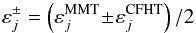 (9)and the index
j running over all
N(θθθc)
galaxies within a distance θout from
. The outcome of
this experiment is shown in Fig. 8: While
ℳ+ (blue contours) retrieves the signal of both clusters (black circles),
exhibiting the expected great similarity to the matched-sources S-maps in
Fig. 7, ℳ− (grey-scale and white
contours in Fig. 8) has a much smaller amplitude. Its
pattern is not obviously related to the one seen in ℳ+: Although the main
clusters reside in a region of enhanced ℳ−, they do not correspond to peaks
in ℳ−. The absence of the ℳ+-peaks in ℳ− is
consistent with the absence of a noticeable shear calibration bias between MMT and CFHT
(cf. Sect. 5.2). A possible explanation for the
stripe-like pattern in ℳ− are differences in the spatially varying anisotropy
correction. We conclude these effects to be small and no impediment to direct comparisons
of MMT and CFHT WL measurements, which we conclude to be consistent.
(9)and the index
j running over all
N(θθθc)
galaxies within a distance θout from
. The outcome of
this experiment is shown in Fig. 8: While
ℳ+ (blue contours) retrieves the signal of both clusters (black circles),
exhibiting the expected great similarity to the matched-sources S-maps in
Fig. 7, ℳ− (grey-scale and white
contours in Fig. 8) has a much smaller amplitude. Its
pattern is not obviously related to the one seen in ℳ+: Although the main
clusters reside in a region of enhanced ℳ−, they do not correspond to peaks
in ℳ−. The absence of the ℳ+-peaks in ℳ− is
consistent with the absence of a noticeable shear calibration bias between MMT and CFHT
(cf. Sect. 5.2). A possible explanation for the
stripe-like pattern in ℳ− are differences in the spatially varying anisotropy
correction. We conclude these effects to be small and no impediment to direct comparisons
of MMT and CFHT WL measurements, which we conclude to be consistent.
The SW peak.
A peculiar feature in the MMT S-map of CL 1701+6414 is the 3.6σ shear peak at αJ2000 = 17h00m05s, δJ2000 = +64°11′00), south-west of A 2246 (cf. Fig. 3). This peak does not correspond to an evident overdensity of galaxies in the MMT and CFHT r′-band images, nor to an extended emission in the Chandra X-ray images. The pure CFHT S-map does not show a counterpart to the SW peak detected with MMT, although the S-contours of A 2246 are extended towards its direction. Interestingly, in the matched-sources S-maps, we detect a 2.8σ peak from the MMT ellipticities and a 2.4σ peak from the CFHT ellipticities. We checked that the SW peak in the MMT S-map does not arise from a chance alignment of a few galaxies with extraordinary high εt resulting from stochastic shape noise. Considering the observations in the CFHT and matched-catalogue S-maps, it seems likelier that we observe a true “shear peak” arising from the superposed light deflections of line-of-sight structure in the complex and dense environment of the CL 1701+6414/A 2246 field.
5.4. Photometric redshift results
Using photo-zs based on the available g′r′i′z′ observations (Table 5) is challenging because of the small spectral coverage and shallowness of the data. Nevertheless, a comparison with sources for which SDSS spectroscopic redshifts are known, revealed a coarse redshift sorting to be possible, with typical errors of σ(zph) ≈ 0.25 for the relevant z ≲ 0.5 redshift range (Appendix C.1). Matching the photo-z catalogue with the CL 1701+6414 MMT data set, we can identify most sources in the galaxy catalogue with a photo-z galaxy, albeit with low quality for most sources (Appendix C.2).
Drawing the S-statistics from this catalogue, whereby galaxies are sorted based on their CFHT photo-zs, we retrieve shear peaks similar to Fig. 3 for the background catalogue, while CL 1701+6414 does not show up as a shear peak in the foreground catalogue (Appendix C.3). From this, we draw two conclusions: First, we likely see an indication of shear emanating from more than one lens plane, namely CL 1701+6414 on the one hand and A 2246 and associated structures on the other hand. Second, owing to the poor quality of the four-band photo-z, a desirable calibration of single-band shear catalogues lies beyond the grasp of this data set.
6. Accuracy of the mass estimates
Weak lensing masses resulting from our analysis.
Components of the statistical error, assuming the B12 mass-concentration relation.
6.1. Error analysis
The error analysis of the seven clusters analysed in Sect. 3 follows the method described in Paper I, i.e. we apply  (10)to
calculate the total uncertainty in mass for each cluster. We will now discuss how we
obtain the different terms in Eq. (10).
The statistical error σstat is inferred from the tabulated
Δχ2 for the cluster on the grid in
r200 and cNFW: taking
Δχ2 = 1, we find the upper and lower limits of
r200 and then applying Eq. (2). Table 6 compares the masses
of our eight clusters and their errors.
(10)to
calculate the total uncertainty in mass for each cluster. We will now discuss how we
obtain the different terms in Eq. (10).
The statistical error σstat is inferred from the tabulated
Δχ2 for the cluster on the grid in
r200 and cNFW: taking
Δχ2 = 1, we find the upper and lower limits of
r200 and then applying Eq. (2). Table 6 compares the masses
of our eight clusters and their errors.
The components σcali and σgeom, accounting for the uncertainties in the shear calibration factor f0 and the redshift distribution of the source galaxies are likewise determined from the analysis of the parameter grid. Assuming the redshift distribution to be well modelled by the fits to the CFHTLS Deep 1 photo-z catalogue, we vary ⟨⟨β⟩⟩ by the uncertainties tabulated in Table 3. As expected, σgeom increases with redshift because of the higher relative uncertainty in ⟨⟨β⟩⟩.
6.2. Redshift distribution
Comparing the source number counts in the CFHTLS Deep 1 field with our MMT data, we find
very good matches to the r′-band source counts in the
CL 0030+2618 and CL 1641+4001 fields, our observations with the deepest limiting
magnitudes and a high density nKSB ≳ 40 arcmin-2
in the KSB catalogues (cf. Tables 1 and 2). The other cluster catalogues exhibit a completeness
limit (peak in the source count histograms) at slightly brighter
r′-magnitudes, but follow the Deep 1 closer than the
corresponding, alternative r+-band source counts from the
COSMOS photo-z catalogue (Ilbert et al.
2009). In order to test for a possible bias in ⟨β⟩ for the
shallower cluster fields, we repeat the fit to the redshift distributions from the four
Deep fields with the following modification: Introducing a magnitude cut, we remove all
galaxies with  from the
CFHTLS catalogues. Virtually independent of zd, we find the
⟨β⟩ for the cases with and without magnitude cut to agree within
mutual error bars for
from the
CFHTLS catalogues. Virtually independent of zd, we find the
⟨β⟩ for the cases with and without magnitude cut to agree within
mutual error bars for  , meaning that the
variation within the Deep fields has the same amplitude as the effect of removing the
faintest sources. In our shallowest field, CL 0230+1836, we measure a limiting magnitude
of
, meaning that the
variation within the Deep fields has the same amplitude as the effect of removing the
faintest sources. In our shallowest field, CL 0230+1836, we measure a limiting magnitude
of  , with 15% of galaxies in the
galaxy shape catalogue at r′ > 25.2.
We thus conclude that no significant bias in ⟨β⟩ is introduced by
using the full Ilbert et al. (2006) catalogue as a
redshift distribution proxy and the dispersion among the four fields as its uncertainty.
, with 15% of galaxies in the
galaxy shape catalogue at r′ > 25.2.
We thus conclude that no significant bias in ⟨β⟩ is introduced by
using the full Ilbert et al. (2006) catalogue as a
redshift distribution proxy and the dispersion among the four fields as its uncertainty.
6.3. Dilution by cluster members
As in the case of CL 0030+2618, we not only consider the uncertainty of ±0.05 we
estimate for f0, but also take into account the dilution by
remaining foreground galaxies in the shear calibration error. Once again using the CFHTLS
Deep 1 photo-z catalogue as a proxy, we determine the fraction of
galaxies
at zph < zcl
after applying the respective background selection. We measure this fraction
to increase with z: it varies from 8.7% for CL 0159+0030 to 32.1% for
CL 0230+1836 (Table 3). As can be seen for
CL 0809+2811 and CL 1416+4446 at the same redshift z = 0.40, the
background selection based on three bands results in a lower
 %
that the mere magnitude cut (
%
that the mere magnitude cut ( %)
for only one band. Adding the two components of the error in quadrature, the lower limit
we consider for f0 ranges from 0.97 for CL 0159+0030 to 0.73
for CL 0230+1836.
%)
for only one band. Adding the two components of the error in quadrature, the lower limit
we consider for f0 ranges from 0.97 for CL 0159+0030 to 0.73
for CL 0230+1836.
6.4. Uncorrelated large scale structure
To calculate the error σLSS induced by LSS, we need to
extrapolate the findings of Hoekstra (2003),
covering only the cases of 5h-1,
10h-1, and
20h-1 × 10¹⁴ M⊙ to lower masses.
(Note that our Mwl estimate for CL 0030+2618 is very close to
the first case.) The respective error contributions read from Fig. 6 of Hoekstra (2003) are
~1.2h-1, ~1.7h-1, and
~2.7h-1 × 10¹⁴ M⊙.
By assuming that the relative LSS error
σLSS/Mwl
increases linearly towards smaller masses, we arrive at the following relation:
 (11)where
a = 0.22h-1, b = −0.01,
and
M14 = Mwl/(1014 M⊙).
We understand Eq. (11) as an
order-of-magnitude estimate for the LSS error and stress that simulated WL measurements
are required to provide a better understanding of this important source of uncertainty. In
particular, we expect a larger σLSS for
higher zd clusters, for which the existence of intervening
massive structure is more likely. We notice that the results of Hoekstra (2003) are obtained at z = 0.3, more nearby
than our clusters.
(11)where
a = 0.22h-1, b = −0.01,
and
M14 = Mwl/(1014 M⊙).
We understand Eq. (11) as an
order-of-magnitude estimate for the LSS error and stress that simulated WL measurements
are required to provide a better understanding of this important source of uncertainty. In
particular, we expect a larger σLSS for
higher zd clusters, for which the existence of intervening
massive structure is more likely. We notice that the results of Hoekstra (2003) are obtained at z = 0.3, more nearby
than our clusters.
In the special case of CL 1701+6414, the obvious LSS at z ≈ 0.22 was taken into account by explicit modelling, in addition to what is described here. We estimate the error associated with the covariance of the parameters describing the two clusters in our simultaneous model for CL 1701+6414 and A 2264 (cf. 4.1) by varying the otherwise fixed r200 of A 2264. The additional error from considering rs,200 = 0.8 Mpc and rs,200 = 1.0 Mpc, according to the uncertainties from our four-parameter fit, give a negligible contribution to the statistical error. Nevertheless, we caution that an additional uncertainty likely arises from our model choice.
6.5. Triaxiality projection bias
Applying the Kasun & Evrard (2005) fitting
formula for the largest-to-smallest axis ratio of a triaxial halo as a function of mass to
all our eight clusters, we arrive at expectation values
of 0.60 < η < 0.64 for
the largest-to-smallest axis ratio. Hence, considering the triaxiality biases of Corless & King (2007), we use
 for the error
Mwl induced by overestimation and
for the error
Mwl induced by overestimation and
 for the one
induced by underestimation caused by the projection of triaxial halos.
for the one
induced by underestimation caused by the projection of triaxial halos.
7. Discussion
The statistical, systematic, and total errors for all eight clusters are summarised in Table 6, both as absolute masses and as relative errors. Table 7 provides the details on the composition of the systematic error for the eight clusters. We note that for all our clusters, in particularly the ones with small WL masses, the statistical uncertainties are the largest component in the total error (the second largest usually being the projection of unrelated LSS). The relative statistical errors range between ≈30% and ≈60%. The reason for this can be twofold: First, the large statistical uncertainties per se are caused by the small signal-to-noise in the lensing signals and thus a consequence of the low net exposure times in the lensing-band images, once we removed frames with high PSF anisotropy (Table 1). Second, our account of the systematics might underestimate or neglect contributions to the systematic error.
For instance, uncertainties in the determination of the centres and the radial fitting ranges are not considered in Eq. (10), which we discuss in Sect. 7.2. After checking the statistical validity of our cluster detection in Sect. 7.1, we evaluate several effects influencing the accuracy with which we can measure weak lensing masses. A reliable quantification of all of these uncertainties is beyond the scope of this article but very desirable with respect to the constraints on cosmology at which the next generation of cluster weak lensing projects is aiming.
7.1. Significance of cluster detections
The S-statistics is known to produce spurious shear peaks even at high significance levels, although as simulations show, false detections above the ~4σ level are rare (e.g., Hetterscheidt et al. 2005; Dietrich et al. 2007). Still, in principle, there is a nonzero, but small chance for one or the other of our detections to be false. Spurious detections are more sensitive against changes in the lensing catalogue or θout. Our tests with different photometric cuts and values for θout found our cluster shear peaks to be robust. Another reaffirmation is the persistence of signals when bootstrapping the lensing catalogue, which we performed for CL 1357+6232, and CL 1416+4446.
In order to test the interpretation of S-values as significances, we conducted the following test: for each galaxy in the catalogue, we add to the phase ϕ of the complex ellipticity estimator ε = |ε| exp(2iϕ) an additional term ϕrnd drawn randomly from a uniform distribution in the interval 0 ≤ ϕrnd < π. This procedure should completely remove the lensing signal from the data such that the resulting value of S be normally distributed around zero, with a standard deviation σ = 1.
We produced 106 realisations of such a randomised catalogue for each cluster and find the S-distributions for all eight cluster detection to be well represented by a Gaussian distribution. In all cases, the absolute of the mean value μ of the fitted Gaussian is |μ| < 0.002, and of the same order of magnitude as the uncertainty in μ derived from the fit. We do not find a bias to either positive or negative S. For six of the eight clusters, we find for the standard deviations σ of the fitted Gaussians values of |1 − σ| < 0.01, with σ = 0.962 and CL 1416+4446 and σ = 0.978 for CL1641+4001, respectively, the largest measured deviations from the expected σ = 1.
For only one cluster, we find one |S| > 5 event among the 106 realisations, consistent with the expectation of one such event in 1.7 × 10⁶ realisations of the expected Gaussian distribution G. Therefore, we conclude that this randomisation test does not find indications for an overestimation of the significance of our cluster detections, as inferred from the S-statistics. On the contrary, the small standard deviations measured from the fits to the CL 1416+4446 and CL1641+4001 correspond to very slightly underestimated significances of these two cluster detections.
7.2. The role of cluster centres
Dietrich et al. (2012) recently demonstrated that the S-peak gives a robust determination of the cluster centre, showing little susceptibility to projected large scale structure (LSS). However, using S-peaks as cluster centres for WL mass estimates is likely to result in a systematic overestimation of cluster masses, because we pick such centres that produce the highest masses. In addition to our default ROSAT centres, we partnered all cluster models with a model choosing the S-peak as cluster centre. While we plan to quantify the centring bias once a more complete sample of our clusters is available, we can show overall trends based on the eight clusters discussed here.
The separations between the shear peaks and ROSAT centres are <3′ in all cases and <1′ for four of the eight clusters (Table 3). This coincidence of X-ray and lensing centres adds further significance to the S-detections. Two out of the four remaining clusters, CL 0159+0030 and CL 0809+2811, have their S-peaks within larger masked areas, reducing the accuracy with which the centres can be determined. The complicated shear fields in the vicinities of CL 1701+6414 and CL 1641+4001, with separations >1′ between lensing and ROSAT centres are discussed in Sects. 4.1 and 4.2. We note that the ROSAT cluster centres themselves are accurate to ~10″.
First, we notice that the S-centred masses are biased high for six of
the eight clusters (squares in Fig. 9). The median is
a 9% higher mass using shear peak centres ( )
than with ROSAT centres (
)
than with ROSAT centres ( ).
We measure
).
We measure  ,
with a 0.36 standard deviation. This indicates the expected presence of a centring bias,
although a small one compared to its scatter.
,
with a 0.36 standard deviation. This indicates the expected presence of a centring bias,
although a small one compared to its scatter.
The most extreme differences are measured for the low-concentration clusters CL 1641+4001
and CL 1701+6414. The sorting in Fig. 9 by increasing
c200 in the S-centred model seems to
suggest a trend of a larger  in
clusters of low concentration. We do not see a similar trend when sorting clusters by
Δθ, the separation between the two types of centres (cf. Table 3), but caution that we deal with small number
statistics. When applying the B01 (B12) mass–concentration relations (big and small upward
and downward triangles in Fig. 9), we arrive at
similar results, with higher median biases of 18% (20%), but still large scatter.
in
clusters of low concentration. We do not see a similar trend when sorting clusters by
Δθ, the separation between the two types of centres (cf. Table 3), but caution that we deal with small number
statistics. When applying the B01 (B12) mass–concentration relations (big and small upward
and downward triangles in Fig. 9), we arrive at
similar results, with higher median biases of 18% (20%), but still large scatter.
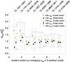 |
Fig. 9 Dependence of weak lensing cluster masses on the choice of centre and mass-concentration-relation. Upward and downward triangles show the masses using the B01 and B12 mass-concentration-relation relative to the case of a free c200. The square and small triangles present models centred on the S-peaks for the free-c200, B01, and B12 cases, respectively. Clusters are ordered by increasing (free) c200 in the S-centred model. Grey lines denote the statistical error bars in the reference model (ROSAT-centred, free c200). |
7.3. Low concentration clusters
As Fig. 9 shows, the relative differences between
masses measured with the six different models for centre and concentration parameter are
most pronounced for CL 1641+4001 and CL 1701+6414, the two clusters with the lowest
intrinsic concentrations  .
.
First we remark, that low values for c200 are neither unexpected nor unheard of in the weak lensing literature (cf., e.g., Oguri et al. 2010; Planck Collaboration 2012). Small concentration parameters as in CL 0809+2811 or CL 1357+6232 are not unique to our analysis method, especially when using a cluster centre significantly offset from the shear peak or in fields affected by masks in the data. Our analysis highlights the importance of such effects.
We note that, using an elliptical NFW cluster model, Oguri et al. (2010) found four out of the 25 X-ray selected clusters they analysed a best-fit cvir < 1. These four extreme cases are among the clusters Oguri et al. (2010) exclude from further analysis for centring problems or obvious misfit of the assumed model. The authors do not, however, report similar problems for three further clusters with 1 < cvir < 2.
The more extreme cases of CL 1641+4001 and CL 1701+6414 point to the limitations of describing a cluster shear field using a single, spherically symmetric function, even if obvious line-of-sight structure like A 2264 is taken into account. Nevertheless, tests like the comparison of κ-maps for CL 1701+6414 from MMT and CFHT (Sect. 5.3) demonstrate that the measured low concentration parameters reflect the reality of the mass distribution and are not artifacts of the analysis. Concerning cosmological applications, the rejection of such clusters will likely result in a biased mass, which we prefer to avoid. We notice that, making different choices in the data analysis, High et al. (2012) likewise succeed in measuring masses of clusters showing a flat shear profile.
7.4. Influence of mass-concentration-relations
Comparing the masses obtained with the three different choices for c200 (free parameter, B01 and B12 mass-concentration relations; Fig. 9 and Table 4), we observe interesting trends. Intrinsically, the B12 relation yields lower concentrations for the same cluster than B01. This relates to the result that the mass assuming B01 exceeds the B12 mass, except for CL 0159+0030. Despite the overall agreement of the masses within their errors, the spread between the two masses seems to decrease with c200, independent of the choice of centre.
On average, using a mass-concentration relation results in a lower mass estimate compared to a free c200, with ~1σ significance for the B01 relation (⟨ M200,B01/M200,def⟩ = 0.85 ± 0.16) and less so for the B12 relation (⟨ M200,B12/M200,def⟩ = 0.95 ± 0.13).
For the S-peak-centred masses, we obtain a similar picture. The B01 masses increase relative to the free-c200 masses, following this trend monotonically despite the statistical uncertainties. In Fig. 9, this can be seen looking at the squares and small upward triangles. The correlation can be explained by the shape found in the confidence contours of most of the clusters for which c200 can be constrained (e.g. CL 1357+6232; Fig. 2): Relatively high values for c200 only agree with the data for r200 smaller than the best-fit value. The underlying reason is the absolute value of the shear signal ruling out simultaneously higher values for c200 and r200.
It will be interesting to see if the tentative trends in Fig. 9 will persist for a more complete cluster sample. We note that due to the substructure and non-sphericity of ΛCDM halos, we expect mass-concentration measured with weak lensing to be biased with respect to the more direct estimates from the simulations (e.g., Bahé et al. 2012). At the current level of eight clusters, all mass estimates agree with each other within their error margins. We notice the relative statistical uncertainties to be only weakly dependent on the choice of c200 (free parameter, B01, or B12 mass-c200-relations).
7.5. Masking of bright stars
Three bright stars exacerbating the analysis of the CL 0159+0030, CL 0230+1836, and CL 0809+2811 fields, identified by their BD and HD designations.
In Table 8, we summarise the properties of the magnitude 8–9 stars that impede the analysis in the CL 0159+0030, CL 0230+1836, and CL 0809+2811 fields. By coincidence, these three most severe cases among the sample of 36 clusters are among our MegaCam targets, reminding us that such fields must not be discarded when analysing a statistically complete sample. Using the example of CL 0809+2811, we study the impact of these stars and their masking on the S-maps and mass estimates.
Removing the masks generated for regions of deviant source density (Sect. 2.2, red squares in Fig. D.3) does not increase the number of usable galaxies significantly: Where
scattered light strongly affects the local background estimation, sources are discarded in
an early stage of catalogue preparation. At the position of the ROSAT centre, there are no
detections in the first place. Without masking, the S-peak of
CL 0809+2811 is shifted by  to the north-east (closer to
the ROSAT centre) and very slightly lower (Smax = 5.27 instead
of Smax = 5.39). Because our default model excises galaxies at
<
to the north-east (closer to
the ROSAT centre) and very slightly lower (Smax = 5.27 instead
of Smax = 5.39). Because our default model excises galaxies at
< separation, to avoid the strong
lensing regime, the impact on the mass is below 2%.
separation, to avoid the strong
lensing regime, the impact on the mass is below 2%.
A more important point could be the extra uncertainty in the chosen cluster centre, as we
find the largest offsets between WL and X-ray peaks for clusters with large masks.
The  observed for CL 0159+0030 (Fig. 9) is likely due to a
washed-out lensing peak. Nevertheless, we do not observe similar peculiarities for
CL 0809+2811.
observed for CL 0159+0030 (Fig. 9) is likely due to a
washed-out lensing peak. Nevertheless, we do not observe similar peculiarities for
CL 0809+2811.
7.6. Further sources of uncertainty
There are several potential sources of uncertainty which are not considered in Eq. (10), for instance, uncertainties in the determination of the centres or the contamination correction available only for clusters imaged in g′r′i′. A reliable quantification of these errors will require further analysis.
We also do not consider the uncertainty in the choice of max(| ε|) in
the error analysis. However, we account for its effect via the shear calibration such that
we do not expect a significant additional systematic error. Carefully calibrated
simulations of cluster lensing are necessary to test our assumptions on the shear
calibration factor. In Paper I, we observed in CL 0030+2618 a counter-intuitive decrease
of the best-fit value for  with
increasing max(| ε|). Indeed, only CL 1357+6232 shows a similar
relative decrease in . Averaging
over all eight clusters, these cases are balanced by CL 0230+1836 and CL 1416+4446, for
which we measure to increase
with max(| ε|). With max(| ε|) = 1.0, we measure
for four cases a smaller than for
max(| ε|) = 0.8, and in four cases a larger radius. The same holds
for max(| ε|) = 104. These results suggest that the
uncorrected bias due to max(| ε|) might be small.
with
increasing max(| ε|). Indeed, only CL 1357+6232 shows a similar
relative decrease in . Averaging
over all eight clusters, these cases are balanced by CL 0230+1836 and CL 1416+4446, for
which we measure to increase
with max(| ε|). With max(| ε|) = 1.0, we measure
for four cases a smaller than for
max(| ε|) = 0.8, and in four cases a larger radius. The same holds
for max(| ε|) = 104. These results suggest that the
uncorrected bias due to max(| ε|) might be small.
We notice that the roles of the shear calibration f0,
considered in Eq. (10) as
σcali and the correction
f1(θ) for cluster members cannot be
completely disentangled. On the one hand, considering the cluster member correction
separately is justified by the radial dependence of
f1(θ). On the other hand, we stress that
the uncertainty in f1(θ) might be large due
to the weak detections of the cluster red sequence. In addition, the effect of cluster
member decontamination on the mass estimate (3% to 7%; up to 11% using shear-peak centres)
lies within the range of the related systematic error component
 which is
significantly smaller than the statistical uncertainty in the mass. Hence, a possible plan
to consider cluster membership consistently – also for single-band clusters – would be to
include it into the systematic error. Again, we suppose performing simulations of cluster
WL fields to be helpful for the further investigations.
which is
significantly smaller than the statistical uncertainty in the mass. Hence, a possible plan
to consider cluster membership consistently – also for single-band clusters – would be to
include it into the systematic error. Again, we suppose performing simulations of cluster
WL fields to be helpful for the further investigations.
Finally, we note that total 1σ error intervals consistent with cluster masses close to zero do not mean these clusters are detected merely at the ~1σ level: shear calibration, zs-distribution, and triaxiality errors are multiplicative, such that they do not affect the detection significance.
8. Summary and conclusion
In this study, the second in the series on the 400d survey WL follow-up, we reduced and analysed MMT/MegaCam observations for seven clusters of galaxies. Building on Paper I, data reduction is performed using THELI, and WL shear catalogues are extracted using an implementation of the KSB+ algorithm.
In the three cases, where we have MMT observations in g′r′i′, we define lensing catalogues based on a refined version of the three-colour method used in Paper I. By comparing with the colours observed for a Ilbert et al. (2006) photo-z field, we exclude sources from regions in colour-colour–magnitude space containing a large fraction of foreground galaxies from the analysis. For clusters with only one MMT band, we apply a cut in magnitude as background selection.
We detect all of our
0.39 < z < 0.80 clusters
using the aperture mass method (S-statistics) at the
>3.5σ level. Performing a Seitz & Schneider (2001) mass reconstruction, we find the
projected mass to follow the S-statistics closely. The WL masses of our
clusters are determined from NFW modelling of their tangential shear profiles, yielding
masses in the 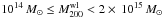 interval.
Two of our clusters are exceptional due to their complicated shear morphology: For CL 1701+6414, where several known clusters lie close to one another in projection, we simultaneously fit the shear of the two strongest S-peaks, identified with A 2246 and our target. The field of CL 1641+4001 also exhibits multiple shear peaks, but we find no evidence for the presence of more than one cluster.
An independent analysis of the CL 1701+6414 field using archival CFHT data confirms the superposition of several weak lensing sources. By matching shear catalogues from MMT and CFHT, we find ellipticities measured with both instruments to be consistent with the assumption of noisy, but unbiased measurements of the same quantity. Hence, MMT/MegaCam is proven to be equally good for WL science as the well-established CFHT/MegaCam. We further produced a photo-z catalogue based on CFHT g′r′i′z′ data of the field. Despite the shallowness of three bands, we are able to devise a coarse foreground/background selection for CL 1701+6414. This experiment again confirms not only shear peaks for several known clusters but also the validity of the magnitude-cut selection. Better photo-z data will be needed to potentially turn this cross-check into a calibration for single-band lensing data.
We find the error budgets for our cluster masses to be dominated by statistical uncertainties (which can be suppressed by using a large cluster sample), but with a significant contribution of systematic uncertainties. Statistical uncertainties are naturally higher for relatively high-z clusters like ours, but the role of data quality (weather and instrumental conditions that led to drastic reductions in data depth) can hardly be overestimated. Our data show weak indications for clusters with low intrinsic concentration to be more susceptible to model choices, such as the concentration parameter or assumed centre.
As the second paper in the 400d WL series, the main results of this study are that:
-
Instrumental effects are well under control.
-
Reliable masses can be obtained in the presence of bright stars close to the cluster centre – an important finding for a successful follow-up of a complete sample!
-
Ground-based WL works at least till z ≈ 0.8.
-
We can correct for extreme cases of massive foreground structures.
-
Clusters of low concentration are a common occurrence in the high redshift, moderate mass population.
Furthermore, we identify areas of possible future improvements of the methods we applied: As observational constraints will forbid complete homogeneity of the data analysis to some degree for each survey. Therefore, better methods to calibrate WL analyses in particular with a different number of available filters need to be developed. This applies specifically to background selection and correction for cluster members.
Concerning the modelling of clusters with complex shear morphology, we point out that low-mass clusters with a strong fraction of disturbed or merging systems will build the bulk of the population observed by deep and wide future surveys like EROSITA or EUCLID. Hence, the question arises how clusters deviating from a simple NFW mass distribution can be weighed most accurately. A possible method is to apply methods that do not assume radial symmetry, e.g. aperture mass techniques. Nevertheless, profile-fitting methods are well established and increasingly well understood. Alternatively, by combining simulational efforts with improved data analysis and modelling, biases resulting from profile assumptions can be corrected. Thus, applying profile fits even to low-signal, merging clusters might prove the best method to measure reliable masses for large cluster samples.
Online material
Appendix A: Photometric calibration details
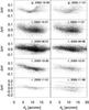 |
Fig. A.1 Accuracy of the photometric calibration: For the different combinations of filters and nights used to calibrate the data sets discussed in this work and Paper I, the scatter Δm′ around the best-fit solution (solid line) is shown. Each point corresponds to an SDSS standard source for which the abscissae give the separation θ0 in arc minutes from the centre of the pointing. Note that for each panel a maximum Δm′ has been determined by iterative 3σ-clipping. |
Applying the Hildebrandt et al. (2006) method,
photometric calibration of our data is established by fitting instrumental
(minst) to reference (mSDSS)
magnitudes for a sample of objects, taking into account variable airmass
a and a colour term cSDSS describing the
transformation between MegaCam and SDSS filter systems:  (A.1)Depending on
the photometric quality of the observations, we fit the zeropoint
Zf together with the parameters
βf or γf in optimal
conditions, or keep γf fixed at the default value depending
on the filter f for poorer conditions.
(A.1)Depending on
the photometric quality of the observations, we fit the zeropoint
Zf together with the parameters
βf or γf in optimal
conditions, or keep γf fixed at the default value depending
on the filter f for poorer conditions.
The resulting values for the fit parameters, as well as the colour indices cSDSS,f for the different filters are presented in Table A.1, for all photometric nights of our MegaCam runs11. We find the zeropoints Zf of the photometric nights to agree among the g′r′i′ filters, with a largest deviation of ≈0.15 mag. The scatter Δm′ = minst − mSDSS + βfcSDSS,f + γfa + Zf of the individual SDSS standards about the best-fit solution (Fig. A.1) has a comparable amplitude. The errors of Zf given in Table A.1 are the formal fitting errors. Figure A.1 presents the data from which the fit parameters have been determined, applying an iterative 3σ-clipping fit of Eq. (A.1).
Comparing the colour terms βf for the different nights, we find considerable agreement within the values for each of the three bands, although the formal errors underestimate the true uncertainties. We suggest that the large span in values of βg might be caused by the known dependence of the filter throughput on the distance to the optical axis. Plotting the scatter Δm′ as a function of the separation θ0 of the source from the optical axis of MegaCam (Fig. A.1), given by the pointing position in the fits header, we can confirm trends of Δm′(θ0) in all filters, most pronounced for the g′ band data taken on 2005 October 30. This trend is likely caused by a combination of the sky concentration effect (position-dependent illumination due to scattering in the telescope optics) and the position-dependent transmissivity of the MegaCam filters, which is strongest in the g′ band (cf. Fig. A.3 in Paper I). A more conclusive investigation of this issue, requiring full propagation of errors on instrumental magnitude, lies beyond the scope of this paper. Because the radial dependence observed in Fig. A.1 does not exceed the residual scatter for sources at the same θ0, the global photometric fits (Eq. (A.1)) fulfil the requirements of our analysis.
Appendix B: Details of background selection
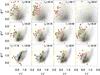 |
Fig. B.1 Fraction of zph ≤ 0.40 galaxies in the Deep 1 (Ilbert et al. 2006) field as a function of
their g′ − r′ and
r′ − i′ colours and
r′ magnitude. Each panel shows a dodecile of the
photo-z catalogue, i.e. one of twelve equally populated
magnitude bins, where the k-th dodecile includes all
galaxies |

In the intermediate magnitude range mbright ≤ r′ ≤ mfaint, our lensing catalogues for three-band clusters include galaxies selected from g′ − r′ versus r′ − i′ colour–colour- diagrams (Sect. 2.4). We find our method justified by considering the Ilbert et al. (2006) photo-z catalogue:
Figure B.1 presents the galaxy numbers and the
fraction of zph ≤ 0.50 sources in the Deep 1
photo-z catalogue as a function of the r′
magnitude and g′ − r′ and
r′ − i′ colours. First, the
catalogue is divided into its dodeciles in r′, i.e. twelve
magnitude bins of equal population are defined where the k-th bin
consists of the galaxies  .
By
.
By  , we denote
the magnitude of a source such there is a fraction
of k/12 of brighter galaxies in the catalogue.
Second, for each dodecile, we show the
number Nij of galaxies falling into grid
cells of mesh
size Δ(g′ − r′) = Δ(r′ − i′) = 0.1,
using a grey scale. Figure B.1 highlights that at
bright r′, only a narrow strip in the colour–colour space
spanned by g′ − r′
and r′ − i′ is populated,
while the locus of galaxies becomes much more diffuse towards fainter
r′. Third, for each grid cell, we determine the fraction
of galaxies we define as foreground sources, i.e. the sources with a redshift estimate
zph ≤ 0.40. The red, green, and blue contours in
Fig. B.1 mark regions of the colour–colour space
populated by 25%, 50%, and 75% of foreground galaxies compared to
the zd = 0.40 clusters, CL 0159+0030 and CL 0809+2811. The
contours are defined such that ffg exceeds the respective
threshold in all grid cells enclosed by the contour.
, we denote
the magnitude of a source such there is a fraction
of k/12 of brighter galaxies in the catalogue.
Second, for each dodecile, we show the
number Nij of galaxies falling into grid
cells of mesh
size Δ(g′ − r′) = Δ(r′ − i′) = 0.1,
using a grey scale. Figure B.1 highlights that at
bright r′, only a narrow strip in the colour–colour space
spanned by g′ − r′
and r′ − i′ is populated,
while the locus of galaxies becomes much more diffuse towards fainter
r′. Third, for each grid cell, we determine the fraction
of galaxies we define as foreground sources, i.e. the sources with a redshift estimate
zph ≤ 0.40. The red, green, and blue contours in
Fig. B.1 mark regions of the colour–colour space
populated by 25%, 50%, and 75% of foreground galaxies compared to
the zd = 0.40 clusters, CL 0159+0030 and CL 0809+2811. The
contours are defined such that ffg exceeds the respective
threshold in all grid cells enclosed by the contour.
As expected, ffg generally decreases towards fainter magnitudes, with only a few zph ≤ 0.40 sources at r′ > 26.0. For all magnitudes, foreground sources with r′ − i′ > 0.5 are rare. In the brightest three dodeciles, a well-defined region with a distinctive edge towards redder r′ − i′ colours exists12 Although the preferred locus of zph ≤ 0.40 galaxies depends little on the r′ magnitude, the zone populated by low-z objects becomes more diffuse for fainter sources. The insignificant role of foreground galaxies r′ > 25.0 justifies that our background selection includes all galaxies fainter than mfaint. Furthermore, the secondary role of mbright compared to mfaint becomes clear from Fig. B.1, noticing the small number of r′ < 20 galaxies.
Calculating ffg for a cluster redshift of
zd = 0.80, the regions in colour–colour space where a
given value of ffg is exceeded extend as well towards
fainter r′ as towards
redder g′ − r′
and r′ − i′ colours.
For zd = 0.80, only a small number of background sources
remain in the first dodecile, while there are significant foreground objects even in
the  bin.
bin.
We adjust our background selection polygon to zd = 0.40 and zd = 0.80 by defining criteria based on ffg > 0.25 contours in the three brightest dodeciles (r′ < 23.91) of the Deep 1 photo-z catalogue (Table B.1 and yellow polygon in Fig. B.1). We exclude galaxies at mbright ≤ r′ ≤ mfaint and matching these criteria from the lensing catalogues. Performing a cross-check for zd = 0.50, we confirm the background selection in Paper I to be sensible, although not optimal. In fact, more “self-calibrations” can be achieved by combining three-colour photometry with photo-z catalogues (Klein et al., in prep.).
Appendix C: Details of photo-z analysis
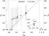 |
Fig. C.1 CFHT photometric redshifts plotted against spectroscopic redshifts from SDSS. The left panel (star symbols) shows the zph for objects identified as stars in SDSS, the middle panel (filled circles) for normal galaxies, and the right panel (filled squares) for QSOs. A small inlay gives a zoomed version for zspec ≈ 0.45 galaxies. The size of the symbols marking the photo-z estimate correspond to the quality parameter o (ODDS): big symbols for o > 0.9, medium-sized symbols for 0.8 < o < 0.9, and small symbols for 0.7 < o < 0.8. Error bars for the zph give the uncertainty interval defined by the BPZ Z_B_MIN and Z_B_MAX parameters. Objects inside a flagged region of one of the CFHT images (CANDMASK = 1) are shown in grey. |
C.1. Spectroscopic calibration
Because our photo-z catalogue for the CFHT CL 1701+6414 field was distilled from only four bands, three of which have rather shallow exposure time (Table 5), we tested its quality by comparison with publicly available SDSS spectroscopy redshifts of the same field. SDSS spectra are only available for a selection of the brightest (r′ ≲ 19) sources, with a total of 88 matches for the ≈270 000 object photo-z catalogue. Out of the 58 sources flagged as good by BPZ in all four filters, 45 are identified as normal galaxies by SDSS, nine are identified as stars, and four as QSOs. Figure C.1 displays zph as a function of zspec of the matched sources for which the BPZ quality parameter ODDS is o > 0.7. The size of the symbols in Fig. C.1 (star symbols for stars, filled circles for normal galaxies, and filled squares for QSOs) corresponds to the value of o.
Generally, the photo-z uncertainties (given by the BPZ Z_B_MIN and Z_B_MAX parameters) are large, although the sources in Fig. C.1 rank among the brightest in the catalogue. Nevertheless, the zph estimates for normal galaxies seem to follow a remarkably narrow and monotonic function of zspec, in the range 0 < zspec ≲ 0.45 probed by the SDSS spectral targets in Fig. C.1. The step at zspec ≈ 0.10, below which galaxies get assigned zph ≈ 0.0 and above which they are overestimated to be at zph ≈ 0.3, can be explained by the lack of a u′ filter crucial for detecting the 400 nm break at these redshifts. In particular, this applies to galaxies in the z ≈ 0.22 structures in the foreground to CL 1701+6414, as exemplified by the zph ≈ 0.40 for one of the A 2246 BCG candidates at zspec ≈ 0.235.
Photo-z estimates for the highest redshift (z ≈ 0.45) galaxies with SDSS spectra are stunningly accurate, despite the large uncertainties. The overall trend seen in Fig. C.1 is consistent with the results of the CFHTLS-Archive-Research Survey (Erben et al. 2009). In their analoguous comparison of CFHT BPZ photo-zs to SDSS spectra, they find a turnover to zph < zspec for zspec ≳ 0.45 (for a small absolute number of such galaxies).
It is a lucky coincidence that the
zph-zspec-relation
intersects the dotted equality line precisely at the redshift of our cluster of
interest. There are six galaxies
0.448 < zspec < 0.457 among
the SDSS spectral targets (inlay in Fig. C.1),
while there are none in the
0.36 < zspec < 0.44
range. These six include the BCG of CL 1701+6414
at zspec = 0.4523 ± 0.0001, for which BPZ
returns zph = 0.45 ± 0.19. However, even the closest of
the other five is separated by  or 4.0 Mpc in projection
and thus not part of or closely interacting with CL 1701+6414. Still,
its zspec = 0.4522 ± 0.0001 indicates they might belong
to the same large-scale structure.
or 4.0 Mpc in projection
and thus not part of or closely interacting with CL 1701+6414. Still,
its zspec = 0.4522 ± 0.0001 indicates they might belong
to the same large-scale structure.
The photo-z estimates for QSOs (right panel of Fig. C.1) are clearly off, which doesn’t come as a surprise as their is no QSO spectrum among the templates employed by BPZ. Although five out of eight stars in Fig. C.1 (left panel) get assigned zph ≤ 0.02, there are also three cases in which our photo-z catalogue suggests higher zph for objects that by visual inspection and SDSS classification clearly stellar: The available CFHT photometry alone does not allow for an accurate star/galaxy classification.
C.2. Matching with MMT
To investigate what benefit the four-band photo-zs yield, once the usual selection of galaxies by magnitude and half-light radius (Sect. 2.4) is applied, we now match the photo-z catalogue with the MMT KSB catalogue. We first notice that although 95.6% of galaxies in the MMT KSB catalogue are matched bijectively to a CFHT photo-z source, only 20.4% of the MMT lensing sources satisfy the quality criteria of four usable CFHT bands (NBPZ_GOODFILT = 4), o > 0.8, and no masking (CANDMASK = 0). We call these estimates high-quality photo-zs.
Counter-intuitive at the first glance, 76% of the high-quality matches have zph > 0.5, i.e. are likely background galaxies to CL 1701+6414. However, this effect can be traced back to the near-absence of high-quality estimates of zph < 0.3. This is consistent with our expectation from the comparison to the spectroscopic redshifts (Fig. C.1), where the lack of a u′ filter systematically offsets zph for zspec < 0.45 galaxies to higher values. The zph distribution derived from the four-band CFHT data deviates far from the redshift distributions known from well-studied photo-z fields (Ilbert et al. 2006, 2009, also see Fig. B.6 in Paper I). This holds in particular for the high-quality sub-catalogue which, containing brighter galaxies on average, traces a different population than our MMT lensing catalogue.
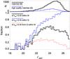 |
Fig. C.2 Upper panel: histograms of the MMT-photo-z matched catalogue as a function of MMT r′ magnitude: Plotted are all matches (thick black line) and the subset of matches with photo-zs passing all quality criteria (“high quality”, blue line). Lower panel: fractions of galaxies zph > 0.45 within: all MMT-photo-z matches (thick black line), the “high quality” matches (blue line), and of high-quality matches zph > 0.45 within all (dashed red line). A thin dotted line gives the magnitude cut at mfaint = 21.9. |
The upper panel of Fig. C.2, showing the magnitude distributions of the high-quality photo-z catalogue (solid blue line) compared to all matches (thick black line) demonstrates that high-quality photo-zs tend to belong to brighter galaxies. This can be seen from the modes of the histograms and is not surprising given the necessary detection in the shallow g′i′z′ images. While 98.5% of the sources in the MMT galaxy catalogue get matched to a photo-z galaxy, only for 26.7% the photo-z passes all quality cuts.
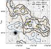 |
Fig. C.3 S-statisics in the CL 1701+6414 field using the CFHT photo-z catalogue. Thick black contours mark the shear signal from the zph < 0.45 catalogue, medium-thick blue contours are derived from the complementary zph ≥ 0.45 sources. Thin orange contours show the signal from the complete MMT galaxy catalogue. All contours start at S = 1 and are spaced by ΔS = 1. The underlying image and other contours are the same as in Fig. 3. |
In particular, the decline with magnitude of the fraction of high-quality matches
affects the fraction of background galaxies with respect to CL 1701+6414 at
z = 0.45 using our photo-zs: considering
high-quality matches only (solid blue curve in the lower panel of Fig. C.2), the fraction of “photometric background”
(zph > 0.45) increases strongly
with MMT r′ magnitude. In fact, all of the few
 high-quality matches show
zph > 0.45. With respect to the
complete catalogue (thick black line), however, the fraction of photometric background
galaxies peaks at
high-quality matches show
zph > 0.45. With respect to the
complete catalogue (thick black line), however, the fraction of photometric background
galaxies peaks at  and ~0.6 and decreases
towards fainter
and ~0.6 and decreases
towards fainter  . The
fraction of high-quality
zph > 0.45 galaxies compared to
all matches (red dashed line in Fig. C.2) runs
rather flat with , never
exceeding 0.3 and subsuming only 15.9% of all matches.
. The
fraction of high-quality
zph > 0.45 galaxies compared to
all matches (red dashed line in Fig. C.2) runs
rather flat with , never
exceeding 0.3 and subsuming only 15.9% of all matches.
We conclude that the quality of the CFHT data entering the photo-z estimation makes possible a rough estimation of a normal galaxy’s redshift, i.e. to decide if it is more likely to be in the foreground or in the background, but not a precise redshift distribiution from which ⟨β⟩ could be inferred more precisely than using a proxy photo-z catalogue of high quality (Sect. 2.5).
C.3. A photo-z shear catalogue
The photo-zs drawn from the CFHT g′r′i′z′ bands provide us with a rough redshift estimate. In order to test whether this information can be used to disentangle the shear signals of CL 1701+6414 and the foreground structure, in particular A 2246, we divide the MMT galaxy catalogue: galaxies with zph < 0.45 are sorted into the “photo-z foreground” catalogue, galaxies with zph ≥ 0.45 are sorted into the “photo-z background” catalogue. Because of the poor quality of most photo-z estimates we expect only a crude selection.
Figure C.3 shows the S-maps resulting from these two catalogues, overlaid on the MMT r′-image in the same fashion as for Fig. 3. Thick black contours denote iso-S-contours from the photo-z background catalogue, including 49.9% of the lensing catalogue (10.3 galaxies/arcmin-2). Solid blue contours in Fig. C.3 are drawn from the complementary photometric foreground catalogue; the signal from the complete galaxy catalogue is shown as thin orange contours.
The morphology of the S-peaks in the photo-z background map follows in its main features the complete catalogue, as we expect from a sample of true z > 0.45 galaxies. With Smax = 3.14, the peak to be associated with CL 1701+6414 is nearly as strong as for the full catalogue, and closer to the cluster’s ROSAT position. The A 2246 peak shows a similar high fraction of the complete catalogue signal, but the two clusters appear to be better separated. The photo-z-foreground S-morphology bears little resemblance to Fig. 3: although we still measure S ≈ 2 close to the position of CL 1701+6414, it can not be seen as a distinct peak. A 2246 is detected just below 3σ, with S > 3 only measured for the “SW peak”. This is consistent with our expectations: As A 2246 is at lower redshift, some signal should persist in a true foreground catalogue.
Re-defining the photo-z catalogue such that it only contains high-quality photo-zs > 0.45 (cf. Sect. C.2) results in a good resolution between the S-signals of the two main clusters but such catalogue suffers from the sparsity of sources (4.8 galaxies/arcmin-2).
Despite the outcome of this experiment matching our expectations, we keep in mind the typical uncertainty of σ(zph) ≈ 0.25 even for the high-quality photo-zs (Fig. C.1), similar to the redshift separation of CL 1701+6414 and A 2246. Hence, the photo-z selection using the available data is not inherently better than the Sect. 4.1 magnitude cut. Nonetheless, the CFHT photo-zs and lensing measurements confirm the detection of CL 1701+6414 as a shear source distinct from A 2246 and give credibility to its mass estimate, the aim of our investigations.
Appendix D: Notes on individual clusters
D.1. CL 0159+0030
Being located in the SDSS equatorial strip, CL 0159+0030 has been detected by Goto et al. (2002) in the SDSS commissioning data, using their photometric “cut and enhance” cluster finder. Plionis et al. (2005) followed up Goto et al. (2002) cluster candidates using archival XMM-Newton observations. From the 3800 s PN observation Plionis et al. (2005) analysed, only a 3σ upper flux limit of 2.1 × 10⁻¹⁴ erg cm-2 s-1 in the 0.5–2.0 keV energy range could be inferred. This non-detection disagrees both with the flux of 3.3 ± 0.4 × 10¹³ erg cm-2 s-1Vikhlinin et al. (2009a) measure for CL 0159+0030 with ROSAT and with their Chandra flux of 3.6 × 10¹³ erg cm-2 s-1 in the same band.
D.2. CL 0230+1836
For CL 0230+1836, there are neither detections of the cluster itself, independent from the 400d survey, nor other galaxy clusters within a 20′ radius listed in NED. To our knowledge, we are the first to study this high-z cluster with deep optical observations.
D.3. CL 0809+2811
We hypothesise that CL 0809+2811 is identical to ZwCl 0806.5+2822 at
αJ2000 = 08h09m34s,
 , a position
 off the CL 0809+2811 ROSAT
centre and at similar distance to the bright star in the field, where we do not see a
concentration of galaxies. Neither do we observe an overdensity of galaxies at the
position of a secondary shear peak with S = 2.9 (Fig. D.3). It is located at
αJ2000 = 08h09m08s,
δJ2000 = +28°05′22″. No cluster within 3′ of this
position is known to NED.
off the CL 0809+2811 ROSAT
centre and at similar distance to the bright star in the field, where we do not see a
concentration of galaxies. Neither do we observe an overdensity of galaxies at the
position of a secondary shear peak with S = 2.9 (Fig. D.3). It is located at
αJ2000 = 08h09m08s,
δJ2000 = +28°05′22″. No cluster within 3′ of this
position is known to NED.
D.4. CL 1357+6232
Lopes et al. (2004) conducted a cluster survey on digitised Second Palomar Observatory Sky Survey plates, using a Voronoi tesselation technique. In their catalogue, they quote a cluster of galaxies at αJ2000 = 13h57m22s, δJ2000 = +62°33′11″, where there is no source in the MegaCam image. Using the relation found between r′ magnitude, g′ − r′ colour and zspec for a subsample of clusters with spectroscopic redshifts, Lopes et al. (2004) assign z = 0.19 to their detection. (NSCS J135722+623311, their #7243). Noting that the position of NSCS J135722+623311 is only 16″ from the ROSAT centre of CL 1357+6232, we speculate that it might be the result of a confusion of CL 1357+6232 with two bright galaxies to its east, one of which (SDSS J135723.83+623246.1) has a measured redshift of z = 0.078.
D.5. CL 1416+4446
In addition to CL 1416+4446, we detect two other shear peaks at > 3σ significance to the west and south-west of CL 1416+4446. Lopes et al. (2004) list a cluster NSCS J141623+444558 in their catalogue which, by NED, is identified with CL 1416+4446. Furthermore, Lopes et al. (2004) detected a cluster of galaxies at αJ2000 = 14h16m09s and δJ2000 = +44°38′51″, with a redshift of z = 0.39. Less than 2′ north-east of these coordinates we find the south-western shear peak which coincides with the g′ = 20.1 galaxy SDSS J141613.33+443951.3. For this source, SDSS (Adelman-McCarthy et al. 2008) quotes a spectroscopic redshift of z = 0.397. Note that the brighter galaxy SDSS J141603.01+443725.1, located 2′ further to the south-west from the Lopes et al. (2004) cluster position has an SDSS zspec = 0.310 and does not correspond to an S-peak.
Barkhouse et al. (2006) detected a galaxy
cluster at  ,
,
 , coincident with the
western shear peak, comparing archival Chandra data to optical
g′r′i′
observations in the Chandra Multiwavelength Project. They assign a
redshift z = 0.427 to the cluster, designated BGV 50. In the same
Chandra observation, Barkhouse
et al. (2006) identified another cluster, BGV 53 at
, coincident with the
western shear peak, comparing archival Chandra data to optical
g′r′i′
observations in the Chandra Multiwavelength Project. They assign a
redshift z = 0.427 to the cluster, designated BGV 50. In the same
Chandra observation, Barkhouse
et al. (2006) identified another cluster, BGV 53 at
 and
and
 and a redshift of
z = 0.452, which does not correspond to a bright galaxy in the
MegaCam image or a peak in the S-statistics.
and a redshift of
z = 0.452, which does not correspond to a bright galaxy in the
MegaCam image or a peak in the S-statistics.
Out of the three confirmed clusters in the field, CL 1416+4446 not only is the only 400d X-ray cluster and the strongest lensing detection, but also appears to be the optically richest system in the MegaCam r′-band image. Therefore, CL 1416+4446 possibly presents the most massive system in a physically interacting super-structure, indicated by the z ≈ 0.40 redshifts of all mentioned clusters. Judging by the X-ray morphology, Vikhlinin et al. (2009a) classify CL 1416+4446 as a relaxed system, though. We conclude that the CL 1416+4446 field qualifies as an interesting candidate for further investigation concerning the existence of a super-cluster.
D.6. Cross-identifications of CL 1701+6414
Vikhlinin et al. (1998), on whose 160d ROSAT catalogue the 400d sample builds (cf. Burenin et al. 2007) detect four clusters in the field: VMF 189 (A 2246), VMF 190 (CL 1701+6414), VMF 191, and VMF 192. In an independent ROSAT analysis, Donahue et al. (2002) detect these same four clusters plus RX J1702+6407, which we do not detect in WL. The redshift of z = 0.7 found for the Donahue et al. (2002) optical counterpart of CL 1701+6414 deviates from the redshift of z = 0.45 measured by Burenin et al. (2007) and all other references. CL 1701+6414 is further listed as RX J1701.3+6414 in the Bright Serendipitous High-Redshift Archival ROSAT Cluster sample (Bright SHARC, Romer et al. 2000).
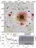 |
Fig. D.1 Like Fig. 2, but for CL 0159+0030. In the plot of r200 against cNFW, a square and dashed contours denote the model minimising Eq. (3) if no dilution correction is assumed. |
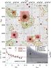 |
Fig. D.2 Like Fig. D.1, but for CL 0230+0030. Note that, in the lower right panel, the filled circle and downward triangle, denoting the best parameters for the free-cNFW abd B12-models are almost coincident. |
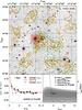 |
Fig. D.4 Like Fig. 2, but for CL 1416+4446. Small star symbols indicate the positions of further clusters in the field, which might be in physical connection to CL 1416+4446 as parts of a super-cluster. |
Their J2000 coordinates are given by the designations in Table 1.
The more common satellite streaks are masked already during the basic data reduction, prior to coaddition.
In addition to the photometric cuts, we restrict ourselves to high-quality sources defined by |ε| < 0.8, SExtractor detection significance ν > 4.5 and tr(Pg) > 0.1 for the KSB pre-seeing polarisability tensor.
Due to the filtering with large scales θout, we measure a signal also in masked areas. Naturally, the correlation between neighbouring grid cells is even higher than in unmasked regions.
We use the fitting formula for ν(M,z) from Table 2 of Bhattacharya et al. (2011).
Due to the high concentration of galaxies, the region is masked.
Strongly overexposed and therefore masked.
For the sake of clarity, we use “MMT” and “CFHT” to distinguish the data sets.
While the good Texp is similar for both data sets, the larger mirror area of MMT is probably offset by the better seeing in the CFHT image.
As the complex ellipticity is the relevant observable, we prefer considering the components of the ratio εMMT/εCFHT over the ratios for the individual components as measured with the two instruments.
Towards very blue r′ − i′ colours, few galaxies are found in the CFHTLS D1 catalogue, basically all of them at low z < 0.4 redshift. This can be seen from the contours in Fig. B.1 which follow the irregular shape of the point cloud. We choose a conservative min(r′ − i′) = − 1.0 limit for the selection polygons.
Acknowledgments
H.I. likes to thank Frank Bertoldi for support of this work and Matthias Klein, Reiko Nakajima, Mischa Schirmer, Ismael Tereno, Bharadwaj Vijaysarathy, Daniela Wuttke, and Yu-Ying Zhang for helpful discussions. Partial support for this work has come from the Deutsche Forschungsgemeinschaft (DFG) through Transregional Collaborative Research Centre TRR 33 as well as through the Schwerpunkt Program 1177. T.H.R. acknowledges support from the DFG through Heisenberg grant RE 1462/5 and grant RE 1462/6. C.L.S. was supported in part by Chandra grants GO9-0135X, GO9-0148X, and GO1-12169X, and by the F. H. Levinson Fund of the Silicon Valley Community Foundation, which helped support the MMT observations. We acknowledge the grant of MMT observation time (program 2007B-0046) through NOAO public access.
References
- Adelman-McCarthy, J. K., Agüeros, M. A., Allam, S. S., et al. 2008, ApJS, 175, 297 [NASA ADS] [CrossRef] [Google Scholar]
- Allen, S. W., Evrard, A. E., & Mantz, A. B. 2011, ARA&A, 49, 409 [NASA ADS] [CrossRef] [Google Scholar]
- Bahé, Y. M., McCarthy, I. G., & King, L. J. 2012, MNRAS, 421, 1073 [NASA ADS] [CrossRef] [Google Scholar]
- Barkhouse, W. A., Green, P. J., Vikhlinin, A., et al. 2006, ApJ, 645, 955 [NASA ADS] [CrossRef] [Google Scholar]
- Bartelmann, M. 1996, A&A, 313, 697 [NASA ADS] [Google Scholar]
- Benítez, N. 2000, ApJ, 536, 571 [NASA ADS] [CrossRef] [Google Scholar]
- Bertin, E., & Arnouts, S. 1996, A&AS, 117, 393 [NASA ADS] [CrossRef] [EDP Sciences] [Google Scholar]
- Bhattacharya, S., Habib, S., & Heitmann, K. 2011 [arXiv:1112.5479] (B12) [Google Scholar]
- Blanchard, A. 2010, A&ARv, 18, 595 [NASA ADS] [CrossRef] [Google Scholar]
- Böhringer, H., & Werner, N. 2010, A&ARv, 18, 127 [NASA ADS] [CrossRef] [Google Scholar]
- Bolzonella, M., Miralles, J., & Pelló, R. 2000, A&A, 363, 476 [NASA ADS] [Google Scholar]
- Bullock, J. S., Kolatt, T. S., Sigad, Y., et al. 2001, MNRAS, 321, 559 (B01) [Google Scholar]
- Burenin, R. A., & Vikhlinin, A. A. 2012, Astron. Lett., 38, 647 [Google Scholar]
- Burenin, R. A., Vikhlinin, A., Hornstrup, A., et al. 2007, ApJS, 172, 561 [NASA ADS] [CrossRef] [Google Scholar]
- Cohn, J. D., & White, M. 2005, Astropart. Phys., 24, 316 [NASA ADS] [CrossRef] [Google Scholar]
- Coleman, G. D., Wu, C.-C., & Weedman, D. W. 1980, ApJS, 43, 393 [NASA ADS] [CrossRef] [Google Scholar]
- Corless, V. L., & King, L. J. 2007, MNRAS, 380, 149 [NASA ADS] [CrossRef] [Google Scholar]
- Corless, V. L., & King, L. J. 2009, MNRAS, 396, 315 [NASA ADS] [CrossRef] [Google Scholar]
- Dietrich, J. P., Erben, T., Lamer, G., et al. 2007, A&A, 470, 821 [NASA ADS] [CrossRef] [EDP Sciences] [Google Scholar]
- Dietrich, J. P., Böhnert, A., Lombardi, M., Hilbert, S., & Hartlap, J. 2012, MNRAS, 419, 3547 [NASA ADS] [CrossRef] [Google Scholar]
- Donahue, M., Scharf, C. A., Mack, J., et al. 2002, ApJ, 569, 689 [NASA ADS] [CrossRef] [Google Scholar]
- Eke, V. R., Cole, S., & Frenk, C. S. 1996, MNRAS, 282, 263 [NASA ADS] [CrossRef] [Google Scholar]
- Erben, T., van Waerbeke, L., Bertin, E., Mellier, Y., & Schneider, P. 2001, A&A, 366, 717 [NASA ADS] [CrossRef] [EDP Sciences] [Google Scholar]
- Erben, T., Schirmer, M., Dietrich, J. P., et al. 2005, Astron. Nachr., 326, 432 [NASA ADS] [CrossRef] [Google Scholar]
- Erben, T., Hildebrandt, H., Lerchster, M., et al. 2009, A&A, 493, 1197 [NASA ADS] [CrossRef] [EDP Sciences] [Google Scholar]
- Goto, T., Sekiguchi, M., Nichol, R. C., et al. 2002, AJ, 123, 1807 [NASA ADS] [CrossRef] [Google Scholar]
- Hartlap, J., Schrabback, T., Simon, P., & Schneider, P. 2009, A&A, 504, 689 [NASA ADS] [CrossRef] [EDP Sciences] [Google Scholar]
- Hetterscheidt, M., Erben, T., Schneider, P., et al. 2005, A&A, 442, 43 [NASA ADS] [CrossRef] [EDP Sciences] [Google Scholar]
- Heymans, C., van Waerbeke, L., Bacon, D., et al. 2006, MNRAS, 368, 1323 [NASA ADS] [CrossRef] [Google Scholar]
- High, F. W., Stubbs, C. W., Rest, A., Stalder, B., & Challis, P. 2009, AJ, 138, 110 [NASA ADS] [CrossRef] [Google Scholar]
- High, F. W., Hoekstra, H., Leethochawalit, N., et al. 2012, ApJ, 758, 68 [NASA ADS] [CrossRef] [Google Scholar]
- Hildebrandt, H., Erben, T., Dietrich, J. P., et al. 2006, A&A, 452, 1121 [NASA ADS] [CrossRef] [EDP Sciences] [Google Scholar]
- Hoekstra, H. 2003, MNRAS, 339, 1155 [NASA ADS] [CrossRef] [Google Scholar]
- Ilbert, O., Arnouts, S., McCracken, H. J., et al. 2006, A&A, 457, 841 [NASA ADS] [CrossRef] [EDP Sciences] [Google Scholar]
- Ilbert, O., Capak, P., Salvato, M., et al. 2009, ApJ, 690, 1236 [NASA ADS] [CrossRef] [Google Scholar]
- Israel, H., Erben, T., Reiprich, T. H., et al. 2010, A&A, 520, A58 [NASA ADS] [CrossRef] [EDP Sciences] [Google Scholar]
- Kaiser, N., & Squires, G. 1993, ApJ, 404, 441 [NASA ADS] [CrossRef] [Google Scholar]
- Kaiser, N., Squires, G., & Broadhurst, T. 1995, ApJ, 449, 460 [NASA ADS] [CrossRef] [Google Scholar]
- Kasun, S. F., & Evrard, A. E. 2005, ApJ, 629, 781 [NASA ADS] [CrossRef] [Google Scholar]
- Komatsu, E., Smith, K. M., Dunkley, J., et al. 2011, ApJS, 192, 18 [NASA ADS] [CrossRef] [Google Scholar]
- Kowalski, M., Rubin, D., Aldering, G., et al. 2008, ApJ, 686, 749 [NASA ADS] [CrossRef] [Google Scholar]
- Kravtsov, A. V., Vikhlinin, A., & Nagai, D. 2006, ApJ, 650, 128 [NASA ADS] [CrossRef] [Google Scholar]
- Larson, D., Dunkley, J., Hinshaw, G., et al. 2011, ApJS, 192, 16 [NASA ADS] [CrossRef] [Google Scholar]
- Lopes, P. A. A., de Carvalho, R. R., Gal, R. R., et al. 2004, AJ, 128, 1017 [NASA ADS] [CrossRef] [Google Scholar]
- Mantz, A., Allen, S. W., Rapetti, D., & Ebeling, H. 2010, MNRAS, 406, 1759 [NASA ADS] [Google Scholar]
- McLeod, B. A., Conroy, M., Gauron, T. M., Geary, J. C., & Ordway, M. P. 2000, in Further Developments in Scientific Optical Imaging, ed. M. B. Denton, 11 [Google Scholar]
- Medezinski, E., Broadhurst, T., Umetsu, K., et al. 2010, MNRAS, 405, 257 [NASA ADS] [Google Scholar]
- Meneghetti, M., Rasia, E., Merten, J., et al. 2010, A&A, 514, A93 [NASA ADS] [CrossRef] [EDP Sciences] [Google Scholar]
- Miller, C. J., Nichol, R. C., Reichart, D., et al. 2005, AJ, 130, 968 [Google Scholar]
- Nagai, D., Kravtsov, A. V., & Vikhlinin, A. 2007a, ApJ, 668, 1 [NASA ADS] [CrossRef] [Google Scholar]
- Nagai, D., Vikhlinin, A., & Kravtsov, A. V. 2007b, ApJ, 655, 98 [NASA ADS] [CrossRef] [Google Scholar]
- Navarro, J. F., Frenk, C. S., & White, S. D. M. 1995, MNRAS, 275, 720 [NASA ADS] [CrossRef] [Google Scholar]
- Navarro, J. F., Frenk, C. S., & White, S. D. M. 1996, ApJ, 462, 563 [NASA ADS] [CrossRef] [Google Scholar]
- Navarro, J. F., Frenk, C. S., & White, S. D. M. 1997, ApJ, 490, 493 [NASA ADS] [CrossRef] [Google Scholar]
- Oguri, M., Takada, M., Okabe, N., & Smith, G. P. 2010, MNRAS, 405, 2215 [NASA ADS] [Google Scholar]
- Pillepich, A., Porciani, C., & Hahn, O. 2010, MNRAS, 402, 191 [NASA ADS] [CrossRef] [Google Scholar]
- Pillepich, A., Porciani, C., & Reiprich, T. H. 2012, MNRAS, 422, 44 [NASA ADS] [CrossRef] [Google Scholar]
- Planck Collaboration 2012, A&A, in press, DOI: 10.1051/0004-6361/201219398 [Google Scholar]
- Plionis, M., Basilakos, S., Georgantopoulos, I., & Georgakakis, A. 2005, ApJ, 622, L17 [NASA ADS] [CrossRef] [Google Scholar]
- Predehl, P., Andritschke, R., Böhringer, H., et al. 2010, in SPIE Conf. Ser., 7732 [Google Scholar]
- Press, W. H., & Schechter, P. 1974, ApJ, 187, 425 [NASA ADS] [CrossRef] [Google Scholar]
- Rasia, E., Ettori, S., Moscardini, L., et al. 2006, MNRAS, 369, 2013 [NASA ADS] [CrossRef] [Google Scholar]
- Reimers, D., Toussaint, F., Hagen, H., Hippelein, H., & Meisenheimer, K. 1997, A&A, 326, 489 [NASA ADS] [Google Scholar]
- Reiprich, T. H. 2006, A&A, 453, L39 [NASA ADS] [CrossRef] [EDP Sciences] [Google Scholar]
- Romer, A. K., Nichol, R. C., Holden, B. P., et al. 2000, ApJS, 126, 209 [NASA ADS] [CrossRef] [Google Scholar]
- Rosati, P., Borgani, S., & Norman, C. 2002, ARA&A, 40, 539 [NASA ADS] [CrossRef] [Google Scholar]
- Sarazin, C. L. 1988, X-ray emission from clusters of galaxies (Cambridge University Press) [Google Scholar]
- Schirmer, M., Erben, T., Hetterscheidt, M., & Schneider, P. 2007, A&A, 462, 875 [NASA ADS] [CrossRef] [EDP Sciences] [Google Scholar]
- Schneider, P. 1996, MNRAS, 283, 837 [NASA ADS] [CrossRef] [Google Scholar]
- Schneider, P. 2006, Weak Gravitational Lensing in: Gravitational Lensing: Strong, Weak and Micro: Saas-Fee Advanced Courses (Springer-Verlag Berlin Heidelberg), 33, 269 [Google Scholar]
- Schneider, P., King, L., & Erben, T. 2000, A&A, 353, 41 [NASA ADS] [Google Scholar]
- Schrabback, T., Erben, T., Simon, P., et al. 2007, A&A, 468, 823 [NASA ADS] [CrossRef] [EDP Sciences] [Google Scholar]
- Schrabback, T., Hartlap, J., Joachimi, B., et al. 2010, A&A, 516, A63 [NASA ADS] [CrossRef] [EDP Sciences] [Google Scholar]
- Schuecker, P. 2005, in Rev. Mod. Astron., 18, ed. S. Röser, 76 [Google Scholar]
- Seitz, S., & Schneider, P. 1996, A&A, 305, 383 [NASA ADS] [Google Scholar]
- Seitz, S., & Schneider, P. 2001, A&A, 374, 740 [NASA ADS] [CrossRef] [EDP Sciences] [Google Scholar]
- Stanek, R., Rasia, E., Evrard, A. E., Pearce, F., & Gazzola, L. 2010, ApJ, 715, 1508 [NASA ADS] [CrossRef] [Google Scholar]
- van Waerbeke, L., Mellier, Y., Radovich, M., et al. 2001, A&A, 374, 757 [NASA ADS] [CrossRef] [EDP Sciences] [Google Scholar]
- Vikhlinin, A., McNamara, B. R., Forman, W., et al. 1998, ApJ, 502, 558 [NASA ADS] [CrossRef] [Google Scholar]
- Vikhlinin, A., Burenin, R. A., Ebeling, H., et al. 2009a, ApJ, 692, 1033 [NASA ADS] [CrossRef] [Google Scholar]
- Vikhlinin, A., Kravtsov, A. V., Burenin, R. A., et al. 2009b, ApJ, 692, 1060 [NASA ADS] [CrossRef] [Google Scholar]
- Voit, G. M. 2005, Rev. Mod. Phys., 77, 207 [NASA ADS] [CrossRef] [Google Scholar]
- von der Linden, A., Best, P. N., Kauffmann, G., & White, S. D. M. 2007, MNRAS, 379, 867 [NASA ADS] [CrossRef] [Google Scholar]
- Wright, C. O., & Brainerd, T. G. 2000, ApJ, 534, 34 [NASA ADS] [CrossRef] [Google Scholar]
- Zhang, Y.-Y., Finoguenov, A., Böhringer, H., et al. 2008, A&A, 482, 451 [NASA ADS] [CrossRef] [EDP Sciences] [Google Scholar]
- Zhang, Y.-Y., Okabe, N., Finoguenov, A., et al. 2010, ApJ, 711, 1033 [NASA ADS] [CrossRef] [Google Scholar]
All Tables
Observation dates, final exposure times and seeing values in the coadded CFHT/MegaCam data for CL 1701+6414.
Components of the statistical error, assuming the B12 mass-concentration relation.
Three bright stars exacerbating the analysis of the CL 0159+0030, CL 0230+1836, and CL 0809+2811 fields, identified by their BD and HD designations.
All Figures
|
Fig. 1 Clusters discussed in this paper. We show pseudo-colour images for the cases where colour is available, using the MMT g′r′i′ bands. For the CL 1701+6414 field, we also show pseudo-colour images using the CFHT g′r′i′ bands, both for CL 1701+6414 and A 2246. We choose the ROSAT cluster coordinates as centre of the images. Note the variable background due to bright stars near CL 0159+0030 and CL 0809+2811. |
| In the text | |
|
Fig. 2 Lensing results for CL 1357+6232. Upper panel: MegaCam
r′-band image (cut-out of ~20′ side length), overlaid
with S-statistics (orange solid) and
|
| In the text | |
|
Fig. 3 Shear signal in the CL 1701+6414 field and its best-fit model with two NFW components accounting for CL 1701+6414 and A 2246. Upper plot: the layout follows Fig. 2. The ROSAT position of A 2246 is marked by a big four-pointed star symbol. Smaller star symbols denote positions of further X-ray clusters. Lower left plot: the layout follows Fig. 2. The solid blue and dashed red lines give the mean tangential and cross shear components, averaged in bins around the CL 1701+6414 shear peak, as expected from the two-cluster model. The separation of the two main clusters is indicated by a vertical dotted line. Lower right plot: the orientations and amplitudes of the shear, as expected from the best-fit two-cluster model, calculated on a regular grid. |
| In the text | |
|
Fig. 4 Simultaneous NFW modelling of CL 1701+6414 and A 2246. Each panel shows the
dependencies between two of the four parameters, with the other two marginalised.
Solid confidence contours (1σ, 2σ,
3σ) denote the default case, using the ROSAT centres; dashed
contours denote models centred on the S-peaks. The respective
parameters minimising |
| In the text | |
|
Fig. 5 Same as Fig. 2, but for CL 1641+4001. In the map, a triangle denotes the secondary shear peak, while a small star symbol marks the position of the von der Linden et al. (2007) cluster candidate. Note that no peak in the complex pattern of shear peaks correlates with its position. |
| In the text | |
|
Fig. 6 Sample density of the ratio εMMT/εCFHT of the complex ellipticities measured for the matched galaxies from the MMT and CFHT r′-band catalogues, respectively. The shaded contours correspond to the logarithmic densities of all galaxies from the MMT lensing catalogue which have a match in the CFHT catalogue. Solid contours give the density of galaxies detected with a signal/noise ratio of ν > 15, the top 32.6%. Note that the normalisation of the ν > 15 galaxies is scaled up by 1/0.326 to obtain the same logarithmic contour levels. A Gaussian smoothing kernel of full-width half-maximum 0.075 was applied to both contour maps. |
| In the text | |
|
Fig. 7 S-statistics in the CL 1701+6414 field drawn from the MMT
(top left), CFHT (top right), and matched
sources catalogues (bottom panels). The linear colour scale,
contours indicating levels of S = 1 to S = 4,
|
| In the text | |
|
Fig. 8 Average and difference aperture mass ℳ ± (Eq. (8)), measured in the matched MMT-CFHT catalogue. The grey-scale and white contours give ℳ−, the thicker blue contours show ℳ+. The spacing for both contours is in multiples of 0.015, starting at 0. Black circles mark the positions of CL 1701+6414 and A 2246. |
| In the text | |
|
Fig. 9 Dependence of weak lensing cluster masses on the choice of centre and mass-concentration-relation. Upward and downward triangles show the masses using the B01 and B12 mass-concentration-relation relative to the case of a free c200. The square and small triangles present models centred on the S-peaks for the free-c200, B01, and B12 cases, respectively. Clusters are ordered by increasing (free) c200 in the S-centred model. Grey lines denote the statistical error bars in the reference model (ROSAT-centred, free c200). |
| In the text | |
|
Fig. A.1 Accuracy of the photometric calibration: For the different combinations of filters and nights used to calibrate the data sets discussed in this work and Paper I, the scatter Δm′ around the best-fit solution (solid line) is shown. Each point corresponds to an SDSS standard source for which the abscissae give the separation θ0 in arc minutes from the centre of the pointing. Note that for each panel a maximum Δm′ has been determined by iterative 3σ-clipping. |
| In the text | |
|
Fig. B.1 Fraction of zph ≤ 0.40 galaxies in the Deep 1 (Ilbert et al. 2006) field as a function of
their g′ − r′ and
r′ − i′ colours and
r′ magnitude. Each panel shows a dodecile of the
photo-z catalogue, i.e. one of twelve equally populated
magnitude bins, where the k-th dodecile includes all
galaxies |
| In the text | |
|
Fig. C.1 CFHT photometric redshifts plotted against spectroscopic redshifts from SDSS. The left panel (star symbols) shows the zph for objects identified as stars in SDSS, the middle panel (filled circles) for normal galaxies, and the right panel (filled squares) for QSOs. A small inlay gives a zoomed version for zspec ≈ 0.45 galaxies. The size of the symbols marking the photo-z estimate correspond to the quality parameter o (ODDS): big symbols for o > 0.9, medium-sized symbols for 0.8 < o < 0.9, and small symbols for 0.7 < o < 0.8. Error bars for the zph give the uncertainty interval defined by the BPZ Z_B_MIN and Z_B_MAX parameters. Objects inside a flagged region of one of the CFHT images (CANDMASK = 1) are shown in grey. |
| In the text | |
|
Fig. C.2 Upper panel: histograms of the MMT-photo-z matched catalogue as a function of MMT r′ magnitude: Plotted are all matches (thick black line) and the subset of matches with photo-zs passing all quality criteria (“high quality”, blue line). Lower panel: fractions of galaxies zph > 0.45 within: all MMT-photo-z matches (thick black line), the “high quality” matches (blue line), and of high-quality matches zph > 0.45 within all (dashed red line). A thin dotted line gives the magnitude cut at mfaint = 21.9. |
| In the text | |
|
Fig. C.3 S-statisics in the CL 1701+6414 field using the CFHT photo-z catalogue. Thick black contours mark the shear signal from the zph < 0.45 catalogue, medium-thick blue contours are derived from the complementary zph ≥ 0.45 sources. Thin orange contours show the signal from the complete MMT galaxy catalogue. All contours start at S = 1 and are spaced by ΔS = 1. The underlying image and other contours are the same as in Fig. 3. |
| In the text | |
|
Fig. D.1 Like Fig. 2, but for CL 0159+0030. In the plot of r200 against cNFW, a square and dashed contours denote the model minimising Eq. (3) if no dilution correction is assumed. |
| In the text | |
|
Fig. D.2 Like Fig. D.1, but for CL 0230+0030. Note that, in the lower right panel, the filled circle and downward triangle, denoting the best parameters for the free-cNFW abd B12-models are almost coincident. |
| In the text | |
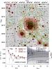 |
Fig. D.3 Like Fig. D.1, but for CL 0809+2811. |
| In the text | |
|
Fig. D.4 Like Fig. 2, but for CL 1416+4446. Small star symbols indicate the positions of further clusters in the field, which might be in physical connection to CL 1416+4446 as parts of a super-cluster. |
| In the text | |
Current usage metrics show cumulative count of Article Views (full-text article views including HTML views, PDF and ePub downloads, according to the available data) and Abstracts Views on Vision4Press platform.
Data correspond to usage on the plateform after 2015. The current usage metrics is available 48-96 hours after online publication and is updated daily on week days.
Initial download of the metrics may take a while.