| Issue |
A&A
Volume 540, April 2012
|
|
|---|---|---|
| Article Number | A73 | |
| Number of page(s) | 17 | |
| Section | Planets and planetary systems | |
| DOI | https://doi.org/10.1051/0004-6361/201118475 | |
| Published online | 28 March 2012 | |
Planetesimal formation by sweep-up: how the bouncing barrier can be beneficial to growth
1 Max-Planck-Institut für Astronomie, Königstuhl 17, 69117 Heidelberg, Germany
e-mail: windmark@mpia.de
2 Institut für Theoretische Astrophysik, Universität Heidelberg, Albert-Ueberle-Str. 2, 69120 Heidelberg, Germany
3 Excellence Cluster Universe, Boltzmannstr. 2, 85748 Garching, Germany
4 University Observatory, Ludwig-Maximilians University Munich, Scheinerstr. 1, 81679 Munich, Germany
5 Department of Earth and Planetary Sciences, Kobe University, 1-1 Rokkodai-cho, Nada-ku, 657-8501 Kobe, Japan
6 Institut für Geophysik und extraterrestrische Physik, Technische Universität zu Braunschweig, Mendelssohnstr. 3, 38106 Braunschweig, Germany
Received: 18 November 2011
Accepted: 16 January 2012
Context. The formation of planetesimals is often accredited to the collisional sticking of dust grains. The exact process is unknown, as collisions between larger aggregates tend to lead to fragmentation or bouncing rather than sticking. Recent laboratory experiments have however made great progress in the understanding and mapping of the complex physics involved in dust collisions.
Aims. We study the possibility of planetesimal formation using the results of the latest laboratory experiments, particularly by including the fragmentation with mass transfer effect, which might lead to growth even at high impact velocities.
Methods. We present a new experimentally and physically motivated dust collision model capable of predicting the outcome of a collision between two particles of arbitrary mass and velocity. The new model includes a natural description of cratering and mass transfer, and provides a smooth transition from equal- to different-sized collisions. It is used together with a continuum dust-size evolution code, which is both fast in terms of execution time and able to resolve the dust at all sizes, allowing for all types of interactions to be studied without biases.
Results. For the general dust population, we find that bouncing collisions prevent any growth above millimeter-sizes. However, if a small number of cm-sized particles are introduced, for example by either vertical mixing or radial drift, they can act as a catalyst and start to sweep up the smaller particles. At a distance of 3 AU, 100-m-sized bodies are formed on a timescale of 1 Myr.
Conclusions. Direct growth of planetesimals might be a possibility thanks to a combination of the bouncing barrier and the fragmentation with mass transfer effect. The bouncing barrier is here even beneficial, as it prevents the growth of too many large particles that would otherwise only fragment among each other, and creates a reservoir of small particles that can be swept up by larger bodies. However, for this process to work, a few seeds of cm-size or larger have to be introduced.
Key words: accretion, accretion disks / protoplanetary disks / stars: pre-main sequence / planets and satellites: formation / circumstellar matter
© ESO, 2012
1. Introduction
One of the most popular planet formation scenarios is based on core accretion, in which the formation of planets starts in the protoplanetary disk with micron-sized dust particles that collide and stick together by surface forces, forming successively larger aggregates (Mizuno 1980; Pollack et al. 1996). Traditionally, the next stage in the formation process is the gravity-aided regime where planetesimals have formed that are so massive that the gravity starts to affect the accretion and the strength of the body.
However, to reach this regime, kilometer-sized bodies are required, something that has proven difficult to produce owing to a number of effects such as fragmentation and bouncing (Blum & Münch 1993), rapid inward migration (Whipple 1972), and electrostatic repulsion (Okuzumi et al. 2011a,b). A new planetesimal formation channel was introduced by Johansen et al. (2007, 2011), in which mutual gravity plays a role between meter-sized boulders in turbulent and locally overdense regions, resulting in the rapid formation of kilometer-sized bodies. However, even the meter regime is difficult to reach only by the coagulation of dust aggregates.
The micron-sized dust particles are coupled tightly to the surrounding gas, and their relative velocities are driven primarily by Brownian motion. Since the resulting relative velocities are small, on the order of millimeters per second, the particles stick together by means of van der Waals forces. However, as the particles increase in size, they become less coupled to the gas, and a number of effects increase the relative velocities between them. For centimeter-sized particles, the predicted relative velocity is already one meter per second, and meter-sized boulders collide at velocities of tens of meters per second. At these high collision energies, the particles tend to fragment rather than stick (Blum & Wurm 2008), which effectively prevents further growth (Dullemond & Dominik 2005; Brauer et al. 2008; Birnstiel et al. 2010).
In the protoplanetary disk, gas pressure supports the gas against the radial component of the stellar gravity, causing it to move at slightly sub-Keplerian velocities. Solid bodies do not, however, experience the supporting gas pressure, and instead drift inward. As the particles grow larger, their relative velocities with respect to the gas increase, causing a significant headwind and a steady loss of angular momentum. At a distance of 1 AU, radial drift can cause meter-sized bodies to spiral inwards and get lost in the star on a timescale of a few hundred orbits (Weidenschilling 1977a; Nakagawa et al. 1986).
These two obstacles give rise to the somewhat inaccurately named meter-size barrier (which ranges from millimeters to meters depending on the disk properties), above which larger bodies have difficulties getting formed. To reach the gravitational regime, bodies that are roughly nine orders of magnitude more massive are needed.
The study of the dust evolution has however until recently primarily been done using simplified dust collision models in which colliding dust grains would either stick together or fragment (Brauer et al. 2008; Birnstiel et al. 2010). The simplicity of the models has been a necessity because of large uncertainties and the small parameter space covered in terms of mass, porosity, and collision velocity in the laboratory experiments and numerical simulations.
Recent years have however seen good progress in the laboratory experiments, as summarized by Blum & Wurm (2008). To provide a more complete and realistic collision model, Güttler et al. (2010) reviewed a total of 19 different experiments with aggregates of varying masses, porosities, and collision velocities. In these experiments, the complex outcome was classified into nine different types. Zsom et al. (2010) implemented this collision model in a Monte Carlo dust-size evolution code. The results showed clear differences from the previous collision models, and allowed for the identification of the most important of the different collision types. They also found the important effect of dust grain bouncing at millimeter sizes that halts the grain growth even before it reaches the fragmentation barrier. With the inclusion of a vertical structure, Zsom et al. (2011) still found bouncing to be prominent, but the vertical settling also allowed for a number of other collision effects to occur.
Progress has also been made with numerical simulations of dust (silica and ice) aggregate collisions using molecular dynamics codes (Wada et al. 2009, 2011) with up to 10 000 monomers corresponding to aggregate sizes of around 100 μm. On the basis of these simulations, Okuzumi & Hirose (in prep.), developed a collision model where growth was possible for silicates for velocities up to 7 m/s, and for ices up to 70 m/s. By incorporating relative velocities in the dead zone extracted from MHD simulations (Okuzumi & Hirose 2011), they were able to form planetesimals made of ice, but not of silicates. Geretshauser et al. (2010, 2011) also developed a dust collision code using SPH for particle sizes of cm and upwards. There is currently a discrepancy between the simulations and the laboratory experiments, where the simulations have difficulties reproducing the bouncing events and generally observe much higher fragmentation threshold velocities. In this paper, we analyze primarily the (more pessimistic) laboratory data, but there is a great need to get the two fields to agree.
One possible way to grow past the fragmentation barrier is so-called fragmentation with mass transfer, which was observed by Wurm et al. (2005) and can happen in a collision between a small projectile and a large target. The projectile is fragmented during the collision and a part of it is added as a dust cone to the surface of the larger particle, provided that the mass ratio of the two particles is large enough to avoid fragmentation of the larger body. The mass transfer efficiency was studied by Kothe et al. (2010), who also showed that multiple impacts over the same area still lead to growth. Teiser & Wurm (2009a,b) showed that growth of the target is possible even for collision velocities higher than 50 m s-1, and Teiser et al. (2011) proved that the target could still gain mass even at high impact angles. These experiments have all shown that dust growth may proceed for large bodies at high velocities, and that this effect might even be able to produce planetesimals via collisional accretion. We discuss this process in more detail in Sect. 2.1.
For the study of the dust-size evolution, the Monte Carlo approach of Ormel & Spaans (2008) and Zsom & Dullemond (2008) has the distinct advantage that it permits the simulation of a large number of particle properties and collision outcomes. A representative particle approach is used where a few particles correspond to larger swarms of particles with the same properties. Each particle is given a set of properties, and each individual collision of the representative particles is followed. This approach uses very little computer memory, and adding extra properties costs very little in terms of execution time. If we wish to study the effect of mass transfer, however, the Zsom et al. approach has some problems, as it only tracks the grain sizes where the most mass can be found in the system. It therefore has difficulties in resolving wide size distributions, which is required for the type of bimodal growth that the fragmentation with mass transfer effect would produce.
Another method is the continuum approach, in which the dust population is described by a size distribution (Weidenschilling 1980; Nakagawa et al. 1981). The conventional continuum approach is the Smoluchowski method, where the interactions between particles of all sizes are considered and updated simultaneously. This leads to very fast codes for a one-dimensional parameter-space (i.e. mass) compared to the Monte Carlo approach. Adding additional properties such as porosity and charge is however very computationally expensive in terms of memory usage and execution time if one does not include steps such as the average-porosity scheme of Okuzumi et al. (2009). With the continuum approach, however, the dust is resolved at all sizes, allowing for all types of dust interactions without any biases. This approach is also fast enough to follow the global dust evolution in the whole disk.
The aim of this paper is to create a new collision model describing the outcome of collisions between dust aggregates of various sizes and velocities, that is fast enough to be used with continuum codes. In this new model, we take into account recent progress in laboratory experiments, especially the mass transfer effect described above, and take a physical approach to transition regions from growth to erosion where the experiments are sparse. We then use this model in size evolution simulations using the local version of the code developed by Birnstiel et al. (2010) to study its implications for the formation of the first generation of planetesimals.
The background of the new model and all the experimental work that it is based on is discussed in Sect. 2, and its implementation is described in Sect. 3. In Sect. 4, we discuss the properties of the disk in our local dust evolution simulations, as well as the implicit Smoluchowski solver that we have used. Finally, in Sects. 5 and 6, we discuss the results of the new model and show how the existence of a bouncing barrier may even be beneficial to the growth of planetesimals.
2. Motivation behind the development of a new collision model
Models to describe the growth of dust aggregates can generally be divided into two parts: a collision model describes the result of a collision between two dust particles of arbitrary properties (i.e. mass, porosity) and velocities. A dust evolution model uses the collision model to describe the evolution of the particle properties of an entire population of dust particles as they collide and interact with each other. In this section, we describe the latest laboratory experiments and our effort to produce a collision model that can take these results into account while still streamlining it to work well with continuum dust evolution codes. That means that the collision model cannot be as complex as the one developed by Güttler et al. (2010), but needs to focus on the most important collision types and aggregate properties. Nevertheless, we were able to include results that were not well-established or even known when the model of Güttler et al. was developed.
2.1. Overview of recent experiments and simulations
Numerous laboratory experiments have been performed to probe the collision parameter space of silicate dust grains, as summarized by Blum & Wurm (2008). This is a daunting task, as planet formation spans more than 40 orders of magnitude in mass and 6 orders of magnitude in collisional velocity and collisional outcomes are affected by for example porosity, composition, structure and impact angle. The classical growth mechanism of dust grains is the hit-and-stick mechanism, which has been well-studied in both laboratory experiments (Blum & Wurm 2000, BW00) and numerical simulations (Dominik & Tielens 1997; Wada et al. 2009). Sticking collisions are also possible via plastic deformation at the contact zone (Weidling et al. 2012, WGB12) and geometrically by penetration (Langkowski et al. 2008, LTB08).
Owing to limited data, previous collision models have with few exceptions only included sticking, cratering, and fragmentation with simplistic thresholds (Nakagawa et al. 1986; Weidenschilling 1997; Dullemond & Dominik 2005; Tanaka et al. 2005; Brauer et al. 2008). To study the effect of the progress in laboratory experiments, Güttler et al. (2010) and Zsom et al. (2010) presented a collision model containing nine different collisional outcomes and used this in the Monte Carlo dust evolution code developed by Zsom & Dullemond (2008). Their model contained three types of sticking collisions in addition to the normal hit-and-stick, and they identified two growth-neutral bouncing effects and three different fragmentation effects in which the largest particle is eroded. They found that several of the new collision types played a role in the dust-size evolution, which proved the necessity for a more complex dust collision approach than previously used. Before even reaching the fragmentation barrier, at which fragmentation events between similar-sized particles prevent further growth, they identified the so-called bouncing barrier. Bouncing collisions between smaller particles of intermediate velocities proved to be an efficient barrier for growth even for grains as small as a millimeter. It should be clarified that bouncing is, in principle, not bad for growth. The bouncing barrier is a problem because of the lack of sticking over such a large range of masses and velocities, which prevents the particles from growing any further.
Bouncing between dust aggregates remains a hotly discussed topic. It has been reported from a large number by laboratory experiments of different setups and material properties (Blum & Münch 1993; Heißelmann et al. 2007; Langkowski et al. 2008; Kelling & Wurm 2009; Güttler et al. 2010; Weidling et al. 2012), but molecular dynamics simulations contain significantly less or no bouncing (Wada et al. 2007, 2008, 2009; Paszun & Dominik 2009). These rebounding events happen in collisions where the impact energy is so high that not all can be dissipated by the restructuring of the aggregates. Wada et al. (2011) argue that this would happen only for very compact aggregates where the coordination number is high, which contradicts what is seen in the laboratory. In the present study, we base our model on laboratory experiments, but bouncing is clearly a very important matter for the dust growth and will need to be investigated in future studies.
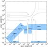 |
Fig. 1 The size-size parameter space of the dust collision experiments (blue boxes) providing the basis for the new collision model. All marked experiments are discussed in more detail in Sect. 2.1. The contours and gray labels mark the collision velocities in cm s-1 expected from the disk model described in Sect. 4.1, and do not always coincide with the velocities studied in the experiments. |
In our new model, we implement the most important collision types identified by Zsom et al. (2010), and also take into account the results of a number of recent experimental studies. Many new experiments have been performed that have increased our understanding of the collision physics of dust aggregates. In Fig. 1, we plot the parameter space of a selection of important laboratory experiments that provide the basis for the new collision model.
Provided that the mass ratio is large enough between the two particles (from now on called the projectile and the target for the smallest and largest particles, respectively), the projectile can fragment and parts of it stick by van der Waal forces to the surface of the target. This was studied by Wurm et al. (2005) and Teiser & Wurm (2009b, TW09b) for millimeter to centimeter-sized projectiles shot onto a mounted decimeter-sized dust target at velocities of up to 56.5 m s-1. It was found that the accretion efficiency even increased with velocity, and could be as high as 50% of the mass of the fragmented projectile, where Güttler et al. (2010) only assumed a constant 2%. This effect was also observed by Paraskov et al. (2007, PWK07) in drop tower experiments where the target also was free-floating without a supported back. The mass transfer efficiency at slightly smaller velocities (1.5–6 m s-1) and for millimeter-sized projectiles was studied in more detail by Kothe et al. (2010, KGB10), who confirmed the velocity-positive trend. Teiser & Wurm (2009a) and Kothe et al. also studied multiple impacts over the same area, and could conclude that growth was possible even then, without the newly accreted material being eroded. It was also found that growth was possible even at very steep impact angles. Beitz et al. (2011, B+11) performed experiments between cm-sized particles at even smaller velocities (8 mm s-1 to 2 m s-1) and detected mass transfer even at velocities as small as 20 cm s-1, right at the onset of fragmentation.
This mode of growth, where small projectiles impact large targets, is related to the work of Sekiya & Takeda (2003, 2005), who performed numerical studies to determine whether small fragments formed in an erosive collision could be reaccreted back onto the target by gas drag. The conclusion was that if the fragments were μm-sized, and the target is sufficiently large, the gas flow would actually compel the fragments to move around the target, thereby preventing reaccretion. For the mass transfer effect, it is important to verify whether this effect could prevent 100–1000 μm-sized projectiles from impacting on the target in the first place. The importance of this effect can be estimated with a simple comparison of timescales using reasonable parameters for the disk model (discussed in more detail in Sect. 4). The stopping time of a small particle is given by 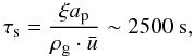 (1)where ξ ~ 1 g cm-3 is the solid density of the projectile, ap ~ 100 μm is its radius, ρg ~ 10-10 g cm-3 is the expected midplane gas density at 3 AU, and
  cm s-1 is the mean thermal velocity of the gas. The time it would take for the projectile to pass the target is given by
  (2)where at ~ 100 cm is a typical target size and Δv ~ 5000 cm s-1 the relative velocity between the particles. Since τs ≫ τpass, it would take too long for the projectile to adjust to the gas flow around the target, and the two particles would collide. If the projectiles were instead only 1 μm in size, the timescales would not differ so much, and the gas flow might play a role.
Another recent experimental result is the refinement of the threshold velocity for destructive fragmentation, where the target is completely disrupted. Beitz et al. (2011) performed experiments to determine the onset of global fragmentation of the particles, and found that cm-sized particles fragmented at 20 cm s-1, much below the 1 m s-1 threshold found for mm-sized particles by Blum & Münch (1993). This points toward a material strength that decreases with mass, as predicted for rocky materials among others by Benz (1999). This result can be explained by a probability of faults and cracks in the material that increases with particle size, and that it is along these cracks that both global breaking and fragmentation takes place. No experiments have as of yet been performed to study the fragmentation threshold of differently sized dust aggregates, but one can generally assume that the velocities needed increase with the size ratio, as seen in both experiments and simulations of collisions between rocky materials (Stewart & Leinhardt 2011; Leinhardt & Stewart 2012).
To provide more data in the transition region between sticking and bouncing, Weidling et al. (2012) studied collisions between particles 0.5 − 2 mm in size and at velocities of 0.1 − 100 cm s-1. In these experiments, sticking collisions were found (in coexistence with bouncing events) for higher velocities than previously expected (Blum & Wurm 2000; Güttler et al. 2010), and enough data now exists to define a transition regime between only sticking and bouncing. Similar experiments with smaller particles roughly 100 μm in size were performed by Kothe (priv. comm.), and are consistent with the threshold of Weidling et al.
Schräpler & Blum (2011, SB11) also performed erosion experiments between μm-sized monomer projectiles and mounted high-porosity aggregates for velocities of up to 60 m s-1, to determine the erosion efficiency as a function of the collision velocity and the surface structure. They discovered that the initial stages of the monomer bombardment are very efficient even at small velocities, but after the most loosely bound monomer chains had been knocked off and the surface had been compacted, the erosion was found to have greatly decreased.
 |
Fig. 2 Sketch of the five possible outcomes described in Sect. 3 sorted in rough order of collision velocity. Mass transfer and erosion act simultaneously in a collision, and we define a mass transfer collision as leading to net growth for the target, and an erosive collision leading to net mass loss. This outcome is extremely dependent on the mass-ratio of the particles, thus adding a second, vertical dimension to the sketch. |
2.2. Individual treatment of collisions
In the collision model of Güttler et al. (2010), a binary approach was used for the particle mass ratios and porosities. Below a certain set critical mass ratio, rc = mt/mp = 10, 100, 1000, the collision was treated as being between equal-sized particles, leading for example to global fragmentation if two large particles collided at high velocities. If the mass ratio was above the critical ratio, the particles were assumed to have different sizes, and a high-velocity collision would instead lead only to cratering. The same approach was taken for the porosity. Below a critical porosity φc = 0.4, a particle was considered to be porous for the purpose of determining the collision outcome, and above it, the particle was assumed compact. Combining these two binary properties gave eight different collision scenarios, where the collision outcome was determined by the particle masses, porosities, and relative velocities.
In the new model, we instead used the current laboratory data to interpolate between the two extreme mass-ratios. This provides a continuous transition from equal-sized to differently sized collisions, and allows us to distinguish between the collisions of particles of different sizes at intermediate mass-ratios, and provides a natural and smooth transition between the two extremes. We can therefore determine the velocity needed to cause global fragmentation for a specific mass-ratio, which gives us a more precise tool to assess when global fragmentation becomes local cratering.
It is however necessary for us to make a simplification regarding the porosity of the dust grains. Adding additional properties to the dust grains is very computationally expensive for continuum codes such as the Smoluchowski solver that we use for the dust-size evolution, compared to Monte Carlo codes. In the Monte Carlo approach, each timestep consists only of one collision between a representative particle and a swarm of identical particles. After the collision, the properties (i.e. mass, porosity, charge) of the representative particle is updated, and a new timestep is initiated. This means that for a simulation with n representative particles, each new property adds only an additional time O(n) to the execution time.
In the Smoluchowski method, one has to numerically solve a number of differential equations to update the number density of all mass bins. For each grain size, n2 interaction terms need to be considered, where n is the number of mass bins. This is because a mass bin can collide with all bins including itself, but fragmentation can also cause mass to be put into it by a collision between two other bins. If an additional property such as porosity were included, m = n porosity bins would need to be included, and for each n·m bin, (n·m)2 interactions need to be considered, and the code would be slower by a factor of O(m3). To include porosity in the Smoluchowski solver, we would therefore require some analytical trick such as an average porosity for each mass bin described in Okuzumi et al. (2009). This is however outside the scope of this paper, and we instead assume that all particles are compact at all times. This is likely a good approximation for larger particles outside the hit-and-stick region, as bouncing collisions quickly lead to compaction of the particles. This finally gives us one single collision scenario, where we can for a collision between any two given particles determine the outcome based on their masses and relative velocities.
3. Implementation of the model
We now describe how the new collision model was created and implemented into the code. We choose to include only the collision types that proved to be the most important in the simulations of Zsom et al. (2010). The collision types considered here are sticking and bouncing as well as the transition between them, mass transfer combined with erosion, and destructive fragmentation. These types are shown schematically in Fig. 2, and discussed in detail in Sects. 3.1–3.3. In Table 1, we provide a summary of all the symbols used in this section.
3.1. Sticking and bouncing thresholds
We consider two dust grains colliding with a relative velocity Δv. The projectile has a mass mp and the target a mass mt ≥ mp. Weidling et al. (2012) found that the mass-dependent sticking and bouncing threshold velocities can be written as ![\begin{equation} \label{eq:stick} \Delta v_{\rm stick} = \left( \frac{ m_{\rm p} }{ m_{\rm s}} \right)^{-5/18}~~~ [{\rm cm~s^{-1} }] \end{equation}](/articles/aa/full_html/2012/04/aa18475-11/aa18475-11-eq27.png) (3)and
(3)and ![\begin{equation} \label{eq:bounce} \Delta v_{\rm bounce} = \left( \frac{ m_{\rm p} }{ m_{\rm b} } \right)^{-5/18}~~~ [{\rm cm~s^{-1} }], \end{equation}](/articles/aa/full_html/2012/04/aa18475-11/aa18475-11-eq28.png) (4)where ms = 3.0 × 10⁻¹² g and mb = 3.3 × 10⁻³ g are two normalizing constants calibrated by laboratory experiments, and the Δv ∝ m−5/18 proportionality is consistent with the theoretical models of Thornton & Ning (1998). The above two thresholds mean that collisions with Δv < Δvstick result in 100% sticking, and Δv > Δvbounce result in 100% bouncing (provided that neither of the particles involved are fragmented). Inbetween these two thresholds, we have a region where both outcomes are possible, as described in more detail in Sect. 3.5.
(4)where ms = 3.0 × 10⁻¹² g and mb = 3.3 × 10⁻³ g are two normalizing constants calibrated by laboratory experiments, and the Δv ∝ m−5/18 proportionality is consistent with the theoretical models of Thornton & Ning (1998). The above two thresholds mean that collisions with Δv < Δvstick result in 100% sticking, and Δv > Δvbounce result in 100% bouncing (provided that neither of the particles involved are fragmented). Inbetween these two thresholds, we have a region where both outcomes are possible, as described in more detail in Sect. 3.5.
Symbols used in the collision model.
3.2. An energy division scheme for fragmentation
From the fragmentation with mass transfer experiments described in the previous section, we assume that mass transfer with a range of efficiencies occurs in all cases where the projectile fragments. If the target also fragments, the mass transfer is negligible compared to the huge mass loss, and we can safely ignore it. We therefore need to determine for each collision whether one, both, or neither of the particles fragment.
The majority of the dust collision experiments have however been performed between either equal-sized or very different-sized particles. To interpolate between these two extremes, we need to consider the collision energy of the event, and determine how this energy is distributed between the two particles. Not only the collision energy of an event matters when determining the degree of fragmentation, but also the mass-ratio between the two particles. In two collisions with equal collision energy but different mass-ratios, we expect the higher mass-ratio collision to be less efficient in completely disrupting the target, as the energy will be more locally distributed around the contact point. To take this into account, we choose to look at the particles in the center-of-mass frame. In this frame, the massive particle moves more slowly than the small one, and during the moment of collision, the kinetic energy of the particles is reduced to zero. Physically, this corresponds to a fully plastic collision where all the energy is consumed by deformation and fragmentation.
In this approach, we assume that the kinetic energy of each particle in the center-of-mass frame will be used to try to fragment itself. The velocities of the two particles in the center-of-mass frame are given by 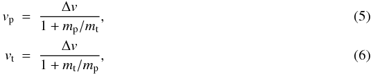 all velocities in the center-of-mass frame will from now on be denoted as v and then mean either vp or vt. The above equations imply that the largest particle has the lowest velocity in the center-of-mass frame. In the case of an extreme mass ratio, mp/mt → 0, the center-of-mass velocity of the projectile and target is given by vp = Δv and vt = 0, respectively.
During a fragmenting collision, the relative size of the largest remnant can be described by 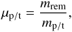 (7)where mrem is the mass of the largest remnant and mp/t the original particle mass. Depending on their sizes and material strengths, the two original particles can be fragmented to different degrees. In this model, each collision partner is treated individually with a μt and μp for the remnant of the target and the projectile, respectively. We define the center-of-mass velocity required for the largest remnant to have a relative mass μ as vμ.
Blum & Münch (1993) and Lammel (2008) studied the threshold velocities needed for two mm-sized particles to fragment with largest remnants of relative masses μ = 1.0 and μ = 0.5, where the former corresponds to the onset of fragmentation and the latter to a largest remnant equal to half of the original particle. Beitz et al. (2011) studied the threshold velocities for cm-sized particles. Interpolating between the results for the two sizes, the center-of-mass frame threshold velocity can be written as ![\begin{equation} \label{eq:frageq} v_{\mu} = (m / m_\mu)^{-\gamma}~~~ [{\rm cm~s^{-1} }], \end{equation}](/articles/aa/full_html/2012/04/aa18475-11/aa18475-11-eq66.png) (8)where mμ is a normalizing constant calibrated by the laboratory experiments and γ = 0.16. The fragmentation threshold velocity is given by v1.0, where m1.0 = 3.67 × 10⁷ g. The velocity required for the largest fragment to have half the size of the original particle is v0.5, where m0.5 = 9.49 × 10¹¹ g. The relative mass of the largest fragment is fitted by a power law that depends on velocity and mass
(8)where mμ is a normalizing constant calibrated by the laboratory experiments and γ = 0.16. The fragmentation threshold velocity is given by v1.0, where m1.0 = 3.67 × 10⁷ g. The velocity required for the largest fragment to have half the size of the original particle is v0.5, where m0.5 = 9.49 × 10¹¹ g. The relative mass of the largest fragment is fitted by a power law that depends on velocity and mass 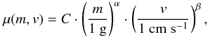 (9)the above equation is valid for all velocities v > v1.0. By fitting the μ(m,v) plane to the two parallel threshold velocities given by Eq. (8), we get
 ![\begin{eqnarray} \alpha &=& \log(2) / \log(m_{1.0}/m_{0.5}) = -0.068, \\ \beta &=& \alpha / \gamma = -0.43, \\ C &= &m_{1.0}^{-\alpha} = 3.27~~~[{\rm g}^{-\alpha}]. \end{eqnarray}](/articles/aa/full_html/2012/04/aa18475-11/aa18475-11-eq76.png) This means that at a larger collision velocity, the particle will fragment more considerably and the size of the largest fragment will decrease. More mass is therefore put into the lower part of the mass spectrum.
This means that at a larger collision velocity, the particle will fragment more considerably and the size of the largest fragment will decrease. More mass is therefore put into the lower part of the mass spectrum.
We can from Eq. (9) determine the largest fragment for each of the particles in the collision, and also use it to identify fragmenting collisions. If μp < 1 and μt ≥ 1, only the projectile fragments and mass transfer occurs. If both μp < 1 and μt < 1, both particles fragment globally. Since the center-of-mass velocity v is inversely proportional to the mass of the particle, we never have a case where only the target fragments and the projectile is left intact, even if vμ decreases with mass.
3.3. A new mass transfer and cratering model
We use a new realistic approach to distinguishing between collisions where the target experiences either net mass gain due to mass transfer, or a net mass loss due to cratering. During each collision, we assume that there is simultaneously:
-
mass added to the target from the projectile via mass transfer;
mass eroded from the target due to cratering.
 (13)where mmt = ϵac·mp is the mass added by mass transfer with the accretion efficiency 0 ≤ ϵac ≤ 1 and mer is the mass lost due to cratering. An increase in the velocity not only leads to increased mass transfer, but also increased cratering. This makes it possible to naturally determine when growth becomes erosion.
The mass transfer efficiency is obtained from Beitz et al. (2011), and depends on both the particle porosity and velocity. Since we are unable to track the porosity of the particles, we assume a constant porosity difference of Δφ = 0.1 between the two dust aggregates, where the target is always the more compact one. This is likely a reasonable approximation for larger particles that have left the hit-and-stick phase and have had time to compact during bouncing collisions, which is the region where mass transfer can be expected. In our prescription, we also include a fragmentation threshold velocity dependence, so that the efficiency is always the same for the same degree of projectile fragmentation. This results in 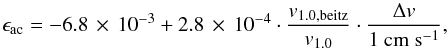 (14)where v1.0,beitz = 13 cm s-1 is the onset of the fragmentation for the 4.1 g particles used by Beitz et al. (2011), and v1.0 is the fragmentation threshold calculated for the mass of the projectile, both calculated using Eq. (8). We here assume a maximum mass transfer efficiency of ϵac = 0.5, as indicated by Wurm et al. (2005). Owing to the process of fragmentation and mass transfer considered here, a higher value would not be reasonable as it would be indicative of complete sticking, which has never been observed at these velocities.
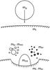 |
Fig. 3 Sketch of the combined cratering and mass transfer process that occurs during a high-enough velocity collision between a projectile with mass mp and a target with mass mt. During the collision, an amount mmt is added from the projectile to the target, and the rest of the projectile is converted into small fragments with a total mass mp,frag. An amount mer is simultaneously eroded from the target, and the final mass of the target is given by |

If the collision energy is not high enough to fragment the particles globally, some of the energy is still used to break up local bonds between monomers around the contact point, resulting in cratering. The cratering efficiency has however only been studied in a couple of laboratory experiments. For monomer projectiles, Schräpler & Blum (2011) found an erosion efficiency given by 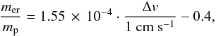 (15)where mer is the amount of eroded mass and mp = m0 is the projectile mass, and m0 = 3.5 × 10⁻¹² g is the monomer mass. Paraskov et al. (2007) studied the erosion of porous targets with both solid and porous projectiles, and found widely results depending on the porosities of the projectile and target. Their results are therefore highly uncertain, but roughly agree with an erosion efficiency of
 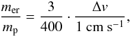 (16)we however note that for the more compact dust aggregates expected after the compression by the bouncing phase, the erosion efficiency should be far lower, as generally seen by Teiser & Wurm (2009b). To interpolate between the two experiments where the degree of erosion has been measured, we assume a mass power-law dependence of
 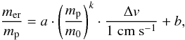 (17)where a, b, and k are fitting parameters. The above two erosion experiments indicate the efficiency of the two different physical effects. In monomer impacts, the projectile hits single surface monomers and sometimes manages to break the bonds between a couple of them. For larger projectiles, restructuring of the target absorbs a lot of the collision energy, and a crater is formed both because of surface compaction and the breaking of monomer bonds. Direct comparisons and interpolations between the efficiencies of the two effects can not be done without huge uncertainties. A direct interpolation between the two effects yields a = 1.55 × 10⁻⁴, b = −0.4, and k = 0.14, but we present below another way of obtaining a reasonable erosion prescription.
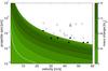 |
Fig. 4 The threshold between growth and erosion from the model compared to the mass-transfer experiments performed by Teiser & Wurm (2009b). Filled circles show experiments where the target gained mass, and open circles where it lost mass. The white dotted line shows the threshold for the highly uncertain erosion prescription from cratering experiments (collisions above the line result in erosion, and collisions below result in growth). The contours are in intervals of 4% net accretion efficiency and mark the region with net growth in the final prescription calibrated using the Teiser & Wurm data. |
As previously discussed, during a collision, erosion and mass transfer usually occur simultaneously, and the net mass change of the target is given by Eq. (13). For Δmt > 0, the target experiences net growth, and for Δmt < 0, the target experiences net erosion. With this prescription, the transition region is extremely sensitive to the efficiency of the erosion.
In Fig. 4, we plot the results of the mass transfer experiments performed by Teiser & Wurm (2009b). We compare this to the threshold between growth and erosion (Δmt = 0) obtained from the mass transfer prescription of Eq. (14) and the erosion prescription of Eq. (17). The threshold derived using the experiment erosion interpolation is given by the white dashed line, and is very pessimistic compared to the mass-transfer experiments.
Since the experimental erosion prescription is obtained from a very different parameter space than we are interested in, it is highly uncertain, and much more so than the mass transfer experiments discussed below. We therefore choose to calibrate the three parameters a, b, and k of Eq. (17) using the experimentally obtained threshold between growth of erosion of Teiser & Wurm (2009b). This results in 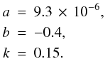 (18)Comparing the net growth efficiency of this fit marked by the contours in Fig. 4 to the mass transfer experiments of Kothe et al. (2010) (with 1 mm projectiles at velocities of 1–6 m s-1) and Wurm et al. (2005) (with 1–10 mm projectiles up to 25 m s-1) results in a rough agreement, even though our model is slightly pessimistic compared to their results, with net efficiencies that are roughly half of theirs. Regardless of this discrepancy, we take this conservative estimate of the experiments and use it for our model.
3.4. Fragmentation distribution
During cratering, mass transfer, and destructive fragmentation events, the mass of each fragmented particle is divided into two parts: the power-law distribution and the largest fragment. The fragment power-law was determined experimentally by Blum & Münch (1993), used in the model of Güttler et al. (2010), and is written  (19)where n(m)dm is the number density of fragments in the mass interval [m,m + dm] , and κ = 9/8.
If the mass of the largest remnant is given by μ·m, where μ is the relative size of the largest remnant described by Eq. (9), the total mass that is put into the power-law distribution is equal to (1 − μ)·m. We define the upper limit to the fragmentation distribution to be min [(1 − μ),μ] ·m. This means that as long as μ < 0.5, we have a single distribution up to the largest remnant. For μ > 0.5, on the other hand, more than half of the mass is put into the largest remnant, which is then detached from the power-law distribution.
 |
Fig. 5 The fragment mass distribution for a 1 cm-sized particle after destructive fragmentation events of varying degrees. The largest remnant is equal to in a) μ = 1, b) μ = 0.9, c) μ = 0.5, and d) μ = 0 in units of the original particle mass. |
This fragmentation recipe is similar to the four-population model of Geretshauser et al. (2011), with the difference that we treat the fragmentation of both particles individually. It is able to describe all different degrees of fragmentation, and in Fig. 5, we present the fragment distribution for four different values of μ. In a), we are at the onset of the fragmentation, and all of the mass is returned to the remnant, leading to no erosion. In b), more than half of the mass is put into the remnant, which is therefore detached from the size distrubution, and in c), the erosion is so strong that the remnant becomes part of the power-law distribution. Finally, in d), the particle is completely pulverized, and all of the mass is converted into monomers.
3.5. Implementation of the model
We now summarize the conditions and outcome of each individual collision type as they have been implemented into the code. The different types are, in order, sticking, transition from sticking to bouncing, bouncing, mass transfer combined with erosion, and destructive fragmentation, and they are all shown schematically in Fig. 2. The conditions for sticking and bouncing are given in Eqs. (3) and (4), and we use Eq. (9) to determine which, if any, of the particles get fragmented during a collision, resulting in fragmentation with mass transfer or destructive fragmentation. Sticking: (Δv < Δvstick). The two particles stick together and form a bigger particle of size mbig = mt + mp. Sticking/bouncing transition: (Δv < Δvbounce). Transition from 100% sticking to 100% bouncing. We assume a logarithmic probability distribution between Δvstick < Δv < Δvbounce given by  (20)where pc is the coagulation probability. At the sticking threshold (Eq. (3)), we know that the sticking probability is pc = 1, and at the bouncing threshold (Eq. (4)), the coagulation probability is pc = 0. The constants are then
  Bouncing: (Δv > Δvbounce), (μp > 1) and (μt > 1), (Δv < ver). If the collision energy is too high to result in a sticking collision but too low to fragment or erode any of the particles, the collision results in a growth-neutral bouncing event. The two masses involved in the collision are left unchanged. This type of collision results in the compaction of both particles, although we ignore any porosity changes in this model. Mass transfer/erosion: (μp < 1) and (μt > 1) or (mer > 0). If the collision velocity is high enough, erosion of the target will occur (Eq. (17)). Simultaneously, if only the projectile fragments, we have a fragmentation with mass transfer event (Eq. (14)). The resulting mass change of the target is given by Eq. (13).
The fragmented mass from the projectile is divided into two parts, a power-law and the largest remnant, with a total mass of m = (1 − ϵac)mp. The power-law distribution has a total mass of mfrag = (1 − ϵac)(1 − μp)mp and the largest fragment a mass mrem = (1 − ϵac)μpmp. The fragments excavated from the target by the cratering are distributed according to a power-law distribution as described in Sect. 3.4, with an upper limit equal to mer. Fragmentation: (μp < 1) and (μt < 1). Finally, if the collision velocity is high enough and the mass ratio not too large, we get a destructive fragmentation event where both particles are fragmented. We treat the fragmentation of each particle individually, and get two separate fragment distributions, one for the projectile and one for the target. Each distribution is divided into two parts; the fragmentation power-law distribution with a total mass of mfrag = (1 − μp/t)mp/t and the largest fragmentation remnant with a mass of mrem = μp/tmp/t.
4. The dust-size evolution model
With the collision model described in the previous section, it is possible to determine the outcome of the collision between any two particles. To study the evolution of the dust in the protoplanetary disk, however, we need to know the properties of the gas and the sources of the relative velocity between the particles. In this section, we describe the disk model used in this paper, along with the dust evolution code of Birnstiel et al. (2010) that has been used together with the new collision model to study the dust-size evolution. A summary of the parameters used for the disk model is given in Table 2.
4.1. The disk model
We follow the dust-size evolution locally at a distance of 3 AU from the star. To describe the gas distribution over the disk, we use the minimum-mass solar nebula (MMSN) model (Weidenschilling 1977b; Hayashi et al. 1985). This model is based on the current Solar System, where the mass of all the planets is used to predict the minimum total mass that would have been needed to form them. It however excludes the effects of both planetary migration and the radial drift of dust grains, and the real initial disk profile might have been much different (Desch 2007). It is however useful for comparison with previous collision models. The gas surface density profile of the MMSN is given by ![\begin{equation} \Sigma_{\rm g}(r) = 1700 \left( \frac{r}{1~{\rm AU} } \right)^{-1.5}~~~[{\rm g~cm^{-2}}], \end{equation}](/articles/aa/full_html/2012/04/aa18475-11/aa18475-11-eq134.png) (23)where r is the distance to the central star. At 3 AU, this results in a gas surface density of 330 g cm-2, and if we assume an initial dust-to-gas ratio of 0.01, a dust surface density of 3.3 g cm-2.
(23)where r is the distance to the central star. At 3 AU, this results in a gas surface density of 330 g cm-2, and if we assume an initial dust-to-gas ratio of 0.01, a dust surface density of 3.3 g cm-2.
We assume four different sources of the relative velocities between dust grains: Brownian motion, turbulence, and both azimuthal and radial drift. Since we use a local simulation at a set point, we take into account the relative velocities that arise, but do not allow the particles to move around in the disk. The different sources are discussed briefly below (see Birnstiel et al. 2010, for a more complete description).
Disk model parameters used in the simulations.
Brownian motion arises from the thermal movement of the particles, and is most effective for the smallest particles. It depends on the mass of the particles as according to  (24)where kb is Boltzmann’s constant, and T = 115 K is the gas temperature that we assume at 3 AU.
Turbulent motion arises from the particle interaction with the surrounding gas, as it is accelerated by turbulent eddies of different size scales. We use the closed-form expressions derived by Ormel & Cuzzi (2007). The turbulence strength is given by the α parameter, which is generally assumed to lie between 10-2 and 10-4. The degree at which different particles are affected by the turbulence is given by the Stokes number, denoting how strongly a particle is coupled to the surrounding gas, which for small particles can be written as  (25)where ξ = 1.6 g cm-3 is the solid density of the dust grains, Σg the surface density of the gas, and λmfp the mean free path of the gas.
Radial drift gives rise to a relative velocity between particles, as they are coupled differently to the surrounding gas (Whipple 1972; Weidenschilling 1977a). This can be written as  (26)where the radial velocity of a particle is given by
  (27)The first term comes from the drag of the surrounding gas on the particle as the gas migrates radially, and vg is the the velocity of the surrounding gas (Lynden-Bell & Pringle 1974). The second term corresponds to the drift of the particle with respect to the gas. Owing to the gas pressure, the gas moves at a slightly sub-Keplerian velocity, and the particle thus experiences a constant headwind, which causes it to lose angular momentum and drift inwards. This effect is strongly related to the coupling between the particle and the gas, where vn representing the maximum drift velocity is derived by Weidenschilling (1977a) as
  (28)and
  is the gas pressure gradient, ρg the gas density, and Ωk the Kepler frequency.
Azimuthal relative velocities are similar to radial drift, and arise from gas drag in the azimuthal direction. The relative azimuthal velocity can be written as  (29)In Fig. 6, we plot the resulting relative velocity field between each particle pair, taking into account the four sources described above. For particles smaller than ~ 10 μm, Brownian motion is the predominant contributor to the relative velocity, causing velocities on the order of mm-1. At larger sizes, turbulence becomes important, and velocities quickly increase to ~ 1 m s-1. As can be seen in Eq. (27), the radial drift is largest for particles with a Stokes number of 1, which at 3 AU corresponds to around 30 cm in size. At roughly this size, owing to the combined effect of radial and azimuthal drift, the particles collide with the smaller particles at velocities of around 50 m s-1, which then decrease to 40 m s-1 as the particles grow larger and the radial drift decreases.
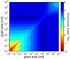 |
Fig. 6 The relative velocities for each particle pair calculated from the four sources described in Sect. 4.1 using the parameters given in Table 2. |
4.2. The Smoluchowski equation
The dust-grain number density n(m,r,z) is a function of the grain mass m, the distance to the star r, and the height above the mid-plane z, and describes the number of particles per unit volume per unit mass. The total dust density can therefore at a point (r,z) be written as  (30)and the change in number density with respect to time can be given by the Smoluchowski equation as
  (31)where M(m,m′,m′′,r,z) is called the kernel, and describes how the mass m is distributed after an interaction between particles of masses m′ and m′′. This distribution is determined by the use of a collision model similar to the one developed in this paper and is described in Sect. 3. Birnstiel et al. (2010) describe how one constructs M from a collision model.
In the code implementation, the density distribution is discretized over logarithmically spaced mass bins. The resulting mass(es) of a collision between two particles will generally not coincide with one specific mass bin. To solve this, the resulting mass is therefore divided between the two neighbouring mass bins by using the Podolak algorithm described in detail by Brauer et al. (2008).
To solve the above equation and track the size-evolution of the dust grains, we use an implicit scheme developed by Brauer et al. (2008) and Birnstiel et al. (2010). This scheme allows for longer timesteps and therefore shorter execution times.
 |
Fig. 7 Comparison between the new collision model (top) and the model of Güttler et al. (2010) (bottom). The left and right panels show the outcome for equal- and differently sized collisions, respectively. Green regions mark collisions that are growth-positive for the target, yellow marks growth-neutral, and red marks growth-negative. “S” marks sticking, “SB” the sticking to bouncing transition, “B” bouncing, “MT” net mass transfer, “E” net erosion, and “F”, fragmentation. In the transition region, the green parallel lines each mark a decrease in sticking probability by 20%. |
5. Results
We performed local simulations of the dust-size evolution using the collision model described in Sect. 3 and the evolution code briefly described in Sect. 4. In this section, we discuss the outcome of the new collision model and compare it to those of previous models. We also show the results of the simulations and compare the growth of the large particles to a simple analytical model.
5.1. The collision outcome space
With the new collision model, we can determine the outcome of a collision between two particles of arbitrary masses and velocities. In the upper panels of Fig. 7, we plot the collision outcome as a function of projectile size and collision velocity for two different mass ratios. This can be compared to the outcome of Güttler et al. (2010) for compact particles shown in the bottom panels. It can here be noted that our model naturally describes the transition between the two extreme cases of equal-sized and differently sized particle collisions, while Güttler et al. defined a critical mass ratio to distinguish between the two regimes. The upper right panel in the figure thus only gives a single snapshot in this transition.
In the left panels, the two particles are of equal size, and the models produce comparable results. In the new model, the sticking region has been enlarged by the inclusion of a transition region where both sticking and bouncing is possible. In the fragmentation region, the mass-dependent fragmentation threshold has decreased the velocity needed to fragment larger particles, and increased the velocity needed for the smallest particles. The net outcome is that the width of the bouncing region has decreased significantly.
In the right panels, the target has a mass that is 1000 times the mass of the projectile. Some important differences can be seen in the fragmentation regime. We can first of all note the new natural transition from growth to erosion that is produced by the balance between growth from fragmentation with mass transfer and erosion from cratering (Eq. (13)). At this mass ratio, erosion quickly becomes complete fragmentation. When the mass ratio is increased yet further, the fragmentation region decreases and is replaced by erosion.
As long as the projectile is fragmenting, velocities below the erosion threshold always cause to growth, and a cm-sized projectile can initiate mass transfer at velocities as small as about 20 cm s-1 (which is exactly the result of Beitz et al. 2011). At Δv = 10 m s-1, projectiles smaller than around 1 cm are required for growth. The maximum projectile size decreases with velocity as the erosion grows stronger, and at Δv = 50 m s-1, growth is only possible for projectiles smaller than 100 μm.
We predict overall more fragmentation and cratering than in the previous model of Güttler et al. (2010). However, one very important change is that growth via fragmentation with mass transfer is now possible at higher velocities than the 20 m s-1 that was the previously predicted threshold, and provided that the projectile is small enough, even a collision at 50 m s-1 as predicted in the disk model can lead to growth of the target (which was a direct conclusion of Teiser & Wurm 2009b).
Sticking collisions are also possible at larger sizes, and growth-positive mass transfer works at much lower velocities than the previously assumed 1 m s-1. Even if the bouncing region shrinks in size, we demonstrate below that this is insufficient to remove the bouncing barrier. If we insert a particle above the bouncing barrier, however, the relative velocity required for it to interact beneficially with the particles below the bouncing barrier has been decreased. These two results turn out to be quite important, as discussed in more detail in Sect. 5.2.
 |
Fig. 8 The collision outcome for all pairs of particles with the relative velocity field calculated in Fig. 6 and with the same labels and color code as in Fig. 7. Also included is the net mass transfer efficiency, given in intervals of 4%. |
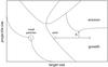 |
Fig. 9 A zoomed-in sketch of the collision outcome space shown in Fig. 8. The dashed horizontal line shows the interaction path that the seed will experience during its growth. The h parameter illustrates the minimum distance between the interaction path and the erosive region. A positive h means that the boulder/small particle interactions will always be growth-positive, and a negative h means that the growth will at some point be stopped by erosion. |
The collision outcome for the new model depends on the mass of both the projectile and the target, and in the current disk model, we use only the average relative velocity between each particle pair. This means that a collision between a given pair in the evolution model always results in the same outcome, and it would therefore be instructive for us to plot the outcome in the particle size-size space. In Fig. 8, we have used the relative velocity field calculated in Sect. 4.1 at a distance of 3 AU to determine the outcome for each collision pair.
In this figure, the bouncing barrier is clearly visible. Owing to the too high collision velocities, dust grains of sizes 100–800 μm that interact with smaller particles will bounce if the particle is not smaller than 10 μm. In this case, a small number of collisions will lead to sticking, but in order to pass the wide bouncing region, a grain would need to experience 109 such sticking collisions. The small particles however themselves coagulate to 100 μm, making growth through the bouncing barrier very difficult.
Collisions between two equal-sized particles larger than 1mm will result in destructive fragmentation, but depending on what it collides with, a 1 mm-sized particle can also be involved in sticking, bouncing, mass transfer and erosive collisions. Owing to the fragmentation with mass-transfer effect, a meter-sized boulder can grow in collisions if its collision partner is of the right size, in this case smaller than 200 μm. As we can see in this plot, the key to growing large bodies is therefore to sweep up smaller particles faster than they get eroded or fragmented by similar-sized collisions.
From Fig. 8, we can already see without performing any simulations that a cm-sized particle would be capable of growing to large sizes if it collides with the right projectiles. The important parameter needed to determine this is illustrated in Fig. 9, which contains a sketch of a part of the collision outcome plot. Because of the bouncing region, most of the particles will be found in the region marked in the figure. A boulder needs to interact beneficially with these bouncing particles in order to grow, so the horizontal interaction path needs to at all times be in the growth-positive mass-transfer region. This can be illustrated with the h parameter, which gives the minimum difference between the interaction path and the erosive region. If h is positive, the boulder will always interact beneficially with the bouncing particles, but if h for some reason were to become negative, the growth of the boulder would stop.
We can now highlight the interesting effect that turbulence has on the collision outcome. For particles of sizes between 10 μm and 10 cm, turbulence is the dominant velocity source. If the relative velocity is higher in this regime, the bouncing barrier will be pushed to smaller sizes. The larger particles are not however as much affected by a stronger turbulence, as these sizes are also affected by both radial and azimuthal drift. This means that the h parameter will remain constant or possibly even increase with stronger turbulence. Strong turbulence might therefore even be beneficial for this mode of growth, as the larger particles will now interact with generally smaller particles, which we from Fig. 4 know promotes the mass transfer effect. Because of this, even if the boulders due to strong turbulence have relative velocities of ~100 m s-1, they can grow in interactions with the small particles at the bouncing barrier, as these have correspondingly decreased in size.
5.2. The dust-size evolution
We performed simulations using the new collision model together with the local version of the Birnstiel et al. (2010) continuum dust-size evolution code. In Fig. 10, the mass distribution of the particle sizes is given at different timesteps for the three different experiments discussed in detail below.
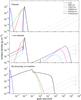 |
Fig. 10 The surface density evolution of the dust population for three different simulations at a local simulation at 3 AU. The gray diagonal lines correspond to the required surface densities for a total number of particles of 1, 103 and 106 in an annulus of thickness 0.1 AU. In the upper panel, all particles initially have a size of 10-4 cm, and snapshots are taken between 2 and 106 years. In the middle panel, we have run the same simulation, but after 10 800 years, a small number of 1 cm-particles have artificially been inserted. In the lower panel, the bouncing barrier has been replaced with sticking, allowing the particles to freely coagulate to larger sizes. |
5.2.1. Growth up to the bouncing barrier
In the fiducial case presented in the top panel, the simulations are initiated using all dust made up of μm-sized monomers. At these small sizes, the relative velocity is driven by Brownian motion, and as the particles collide with each other, they stick together and form larger aggregates. This leads to a rapid coagulation phase where the aggregates grow to 100 μm in around 1000 years. At this point, the particles have grown large enough to become affected by the turbulence, which quickly increases the relative velocities. As we predicted in Fig. 8, the bouncing region is too wide to be surpassed, and the growth halts at the bouncing barrier.
At this stage, the only particles that can grow are the smaller ones, and as time proceeds, more and more particles get trapped at the bouncing barrier. This causes the number of small particles to continue decrease, leading to a continuously narrowing size-distribution. After 105 years, virtually all particles can be found to have sizes of 100 μm, with very steep distribution tails between 60 and 300 μm. If nothing else is done, this is how the dust evolution ends. The bouncing barrier efficiently prevents any further growth, and all particles remain small.
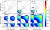 |
Fig. 11 The collision frequency map for the scenario where 1 cm-particles are artificially inserted at t = 10 800 years. The interaction frequency is plotted for each particle pair at six different timesteps plotted on top of the collision outcome space of Fig. 8. This makes it possible to identify the dominating interaction for each particle size. Note the persistently high peak of interactions with particles stuck below the bouncing barrier at 1 mm in size. As the large particles grow, they also sometimes collide among themselves, producing a tail of particles capable of also sweeping up the bouncing particles. This causes an increase in both mass and number for the large particles, and a continuous widening of the size-distribution. |
5.2.2. A seeding experiment
To investigate the potential of the mass transfer effect, we performed an experiment where a very small number (i.e. 10-18 of the total mass) of 1 cm-particles are artificially inserted as “seeds”. As can be seen in Fig. 8, the interaction between the 1 cm and 100 μm-particles results in mass transfer and growth of the larger particle, and we expect the inserted particles to be able to grow. The seeds are inserted at a single time t = 10 800 years, when the particles have reached the semi-stable state at the bouncing barrier, and the result can be seen in the middle panel of Fig. 10. Exactly how the seeds are formed will not be discussed in this paper, but given the small number of seeds required, stochastic effects, small variations in local disk conditions or grain composition and/or properties might suffice to produce them. Some other possibilities are briefly discussed in Sect. 5.4.
To better understand the complex interaction between all the particles in this experiment that now follows, we introduce the collision frequency plot given in Fig. 11. This shows the collision frequency between each particle pair plotted on top of the collision outcome map of Fig. 8, making it possible for any given time to identify the dominating collision type for a given particle size.
The first two snapshots in the collision frequency plot are taken after 2 and 5900 years, and are identical to the fiducial case discussed earlier. At the bouncing barrier, we can see some interaction between the 200 μm particles and the smallest particles that do lead to growth, but the frequency is much too small to have any significant effect.
After 10 800 years, the 1 cm seeds are inserted, and they grow to larger boulders by sweeping up the small particles trapped at the bouncing barrier. As the boulders grow, one can after ~200 000 years see a tail of particles with intermediate sizes appear behind them. These are formed by the rare collisions between the large boulders, and from a single event, two large bodies have been multiplied to a myriad of fragments also capable of sweeping up the particles at the bouncing barrier. This effect causes the population of boulders to not only grow in total mass, but also in number, which causes a steady and significant increase in similar-sized fragmentation.
It can also be noted how the vertical distribution of dust around the midplane affects this stage of the evolution. Even if there is a huge amount of particles trapped at the bouncing barrier, they are so small that many of them are pushed out from the midplane due to turbulent mixing. The boulders are however so large that they have decoupled significantly from the gas, and are therefore mostly trapped in the midplane. This causes the sweep-up rate of the mm-sized particles by the boulders to be distinctly lower than without a vertical structure, and also the internal collisions between the boulders to be relatively more common.
The smallest particles that are produced by global fragmentation and erosion mainly experience two different interactions. In the early stages, the smallest fragments are generally being swept up by the 100 μm-sized particles stuck at the bouncing barrier, since these particles dominate completely both in number and mass. They have therefore never any time to coagulate to larger sizes themselves, but instead aid in the growth of the bouncing particles, which are in turn swept up by the boulders. At later stages, as the boulders become more numerous, it is also possible that the smallest fragments are swept up directly by the boulders. If this growth continues even longer, the two effects become equally efficient, and even later, the boulders will start dominating in the sweep-up. Regardless of what sizes the small fragments interact with, in the end, they are still beneficial for the growth of the boulders.
In the end, a number of 10–70 m boulders have managed to form, and the total amount of mass in the large particles has increased by the huge factor of 1012 from what was initially inserted into the system, even though the total boulder mass is still very small compared to the total dust mass. We find that the limiting case for the growth at this point is not so much erosion or fragmentation as it is the growth timescale (see also Johansen et al. 2008). If the simulation runs for longer than 106 years, the boulders can keep on growing and several hundred-meter boulders can form. In other places in the disk with higher dust densities and relative velocities, larger boulders will be able to form on the same timescale.
Growth by sweep-up gives us an explanation of how the collision part of the growth barrier can be circumvented, but we have in these simulations disregarded the effect of the orbital decay from gas drag. The growth timescales in Fig. 10 exceed by several orders of magnitude the lifetime of meter-sized bodies subject to radial migration. To survive, the bodies need to either form on a timescale very much shorter than observed in our simulations, which we find unlikely, or some effect needs to exist that prevents the orbital decay over an extended period of time (Barge & Sommeria 1995; Klahr & Henning 1997; Brauer et al. 2007; Pinilla et al. 2012).
5.2.3. Removing the bouncing barrier
To illustrate the importance of the bouncing barrier, we devised an experiment in which all the bouncing collisions are removed and replaced by sticking. There is therefore nothing that prevents the coagulation phase from continuing to larger sizes. The results of this simulation are shown in the lower panel of Fig. 10.
The particles can now grow unhindered until they reach about 1 mm in size. At this point, they begin to fragment among themselves, as we can see in Fig. 8. Since most of the dust can be found at this size, heavy fragmentation occurs, and a cascade of smaller particles are produced. These small particles again grow up to larger sizes, where most of them again fragment. From the collision outcome plot, we can however see that some particles can be lucky, and instead sweep up only smaller particles via mass transfer. They therefore avoid fragmentation, and keep on growing, and form the distribution tail extending from 1 mm and upwards.
At a size of roughly 1 m, the only way to grow is by colliding with 100 μm or smaller particles. However, in the absence of a bouncing barrier, most of the mass is found instead in 1 mm particles. This means that almost all of the interactions become erosive, and the growth halts.
In the above example, we saw that increasing the stickiness of particles in the end actually prevented the growth of large boulders. From this result, we can draw the conclusion that the bouncing barrier might even be beneficial for the formation of planetesimals. By hindering the growth of most particles, growth might be possible for the lucky few.
5.2.4. The effect of turbulence
We have so far studied only one single turbulence parameter of α = 10-3. This value is however uncertain for nebular models, and to investigate the dust evolution in different velocity fields, we also study the cases of α = 10-4 and α = 10-2. The latter represents a strong turbulence that completely predominates over the azimuthal and radial drifts and results in relative velocities up to 100 m s-1. In the former case, the turbulence is weak, and contributes very little to the velocities of the larger particles. In Fig. 12, we plot the resulting size evolutions for the three turbulence parameters but otherwise identical initial conditions. The middle panel is here the same as the middle panel of Fig. 10 and included for reference.
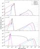 |
Fig. 12 The surface density evolution of the dust population for three different turbulence strengths (α = 10-4,10-3,10-2) at 3 AU, with seeds inserted artificially after t = 10 800 years. |
It can first of all be noted that growth to larger sizes is possible even in the case of very high turbulence, as we predicted using Fig. 9. This is due to the decrease in size of the bouncing particles as the turbulence increases. The smaller impacting projectiles can therefore cause the boulder to grow also at higher velocities, as seen in Fig. 4.
The growth timescale is affected by the turbulence in several different ways. Firstly, it increases the relative velocities between the particles, leading to higher collision frequencies and therefore to more rapid growth. Higher impact velocities also lead to a higher net mass transfer efficiency, which in Fig. 4 is seen to be particularly low for velocities below 10 m s-1. A higher turbulence also mixes small particles further away from the midplane, which decreases their midplane densities where the largest boulders gather, lowering the growth rate. From Fig. 12, it is clear that the growth-positive effects predominate, leading to enhanced growth at higher turbulence. In the low turbulence case, the growth is especially slow for particles of sizes between 1 cm and 100 cm. In this regime, the relative velocities are very low since the contributions from the azimuthal and radial drift are small, causing very low net mass accretion efficiencies during the sweep-up growth.
In the α = 10-2 case, we can see in the final snapshot that a separate peak has appeared for the largest boulders. This peak occurs when the boulders have fragmented so much between themselves that the large intermediate-sized fragments are at number densities roughly equal to the boulders, which in this case happens after ~600 000 years. At this point, the boulders are significantly eroded and fragmented, which creates even more intermediate-sized particles capable of yet more fragmentation. This results in a fragmentation cascade, and a rapid flattening of the size-distribution. This does not however cause all the large particle to be destroyed, and those that survive can continue to grow by sweeping up the small bouncing particles that still dominate both in terms of number and total mass. This effect also occurs for the cases of weaker turbulence if the simulations run long enough, but is never severe enough to cause a complete halt of the growth.
We have demonstrated that growth can also proceed in regions of high turbulence. An MRI turbulent disk might however also create an additional velocity source, where local gas density fluctuations can excite the orbital eccentricities of the planetesimals. Ida et al. (2008) found that this can lead to velocities beyond break-up even for small planetesimals, although they studied only collisions between equal-sized bodies. In our model where only the material strength of the body is included, a collision between two large and similarly sized bodies will be destructive even in regions of very low turbulence, such that in this regime, it has little effect on our conclusions. Excited planetesimal orbits however also increase the impact velocities of the small particles, which could pose a problem. In previous cases, growth had been possible in regions of high turbulence because the sizes of the bouncing particles were simultaneously suppressed by the turbulence, but this is not necessarily the case in the scenario studied by Ida et al. This might cause greater erosion of the growing planetesimals, but investigating this further is beyond the scope of this paper.
5.3. A simple analytical model
To verify the results of our simulations, where growth is caused by the sweeping-up of small particles by a few lucky seeds, we develop a simple analytical growth model in a similar fashion to Johansen et al. (2008) and Xie et al. (2010). We consider a scenario where a single large body of mass m moves around in a sea of small particles of mass ms stuck at the bouncing barrier. The growth of the large body can then be described by  (32)where
  is the collisional cross-section, Δv the relative velocity, ns the number density of the small particles, and ϵnet the average net mass-gain efficiency of a collision. The change in size a with respect to mass can be written as dm = 4πξa2 da, where ξ = 1.6 g cm-3 is the internal density of the large body. We can now write
  (33)where ρs = nsms is the mass density of the small particles. For now, we assume that the relative velocity is only caused by turbulence, and for small particles can therefore be estimated by (Weidenschilling & Cuzzi 1993; Cuzzi et al. 2001)
  (34)where α = 10-3 is the turbulence parameter, St the Stokes number for the boulder given by Eq. (25), and cs the sound speed in the gas given by
  (35)where kb is Boltzmann’s constant, T = 115 K the temperature of the gas, μ = 2.3 the mean molecular weight, and mp the mass of a proton.
We assume ρs to be constant and unaffected by the sweeping-up of the large boulder. When the boulder has grown large enough, it is hardly affected by the vertical mixing from turbulence, and is mostly found near the midplane. We therefore take ρs = 10-12 g cm-3 to be the midplane density assuming a Gaussian vertical profile with a surface density Σs = 3.3 g cm-2 and that all the dust mass can be found in the small particles. Eq. (33) can then be solved analytically  (36)In Fig. 13, we plot the above analytical solution of the boulder growth assuming ϵnet = 0.006, which is the expected efficiency for the interaction between a 1 cm and a 1 mm body. We assume that the other parameters are identical to those in the simulations. This was compared to the observed growth of the largest particle from the seeding simulations in Sect. 5.2.2 using the full collision model. As can be seen, our analytical solution compares well to the growth rate of the simulations for the first stage of growth, and then at later stages differs greatly.
This is due to mainly two reasons. Assuming a constant ϵnet means that at larger sizes it will be underestimated, as in the full model it depends on the collision velocity and varies between 0 and 0.15. The relative velocity prescription in Eq. (34) only takes into account the turbulence, and is also not valid for large particles. In order to take this into account, we use the full net growth efficiency from Eq. (13) and all four velocity sources discussed in Sect. 4. We then solve Eq. (33), and plot the resulting solution in Fig. 13. The new solution and the simulation results now agree very well, only to differ slightly at the largest particle sizes.
We found that this enhanced growth is triggered by the existence of the tail of intermediate-sized particles that form from fragmenting events between large bodies. The largest boulders found in the simulations are those that manage to grow by avoiding interactions with other large bodies. When they manage to interact beneficially with some of the intermediate-sized fragments, the growth rate increases.
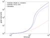 |
Fig. 13 The growth of a boulder in the simulations (black) compared to two growth estimates. The red line corresponds to the simplified analytical estimate, and the blue line to the estimate using the full relative velocity and accretion efficiency prescriptions. |
5.4. Forming the first seeds
The width of the bouncing barrier has been found in recent sticking and fragmentation experiments to be smaller, but still prevents particles from exceeding its limit. As previously discussed, this might even be positive for the planetesimal formation, as it prevents too many large bodies from forming, keeping them from fragmenting and eroding among themselves. It is however necessary for some cm-sized seeds to form and initiate the sweep-up.
In this work, we have found that the bouncing barrier can be circumvented, and growth via mass transfer initiated, even if only a very small number of cm-sized particles is introduced into the system. In this paper, we have not investigated in detail how this might happen, but there are many possibilities. Larger particles may form outside the snow-line mixed with ices, and drift inwards to a region where sweep-up becomes possible. Calcium- and alumunium-rich inclusions (CAIs) are cm-sized particles that are believed to have been formed early near the Sun and transported outwards within the disk (Ciesla 2009), and might also have constituted the first generation of seeds.
It is also possible that some lucky particles grow through the barrier simply by interacting with a sufficient number of smaller particles, as can be seen in the collision outcome plot in Fig. 8. For this to happen, however, it is necessary to have a wide enough size-distribution for there to be enough small particles for the lucky particles to interact with. This, it turns out, is difficult, as we have in these simulations found that the particle size-distribution will quickly narrow as all the small dust coagulate up to the bouncing barrier. If extra mass is continuously introduced into the system during the first 10 000 years or so, for example by the nebular infall of the collapsing protostellar cloud, the particle size-distribution could be wide enough for some seeds to be formed. Beitz et al. (2012) also found in laboratory experiments that chondrules and dust aggregates tend to stick at higher velocities than collisions between two dust aggregates, so that early chondrules could grow where dust could not.
Another possibility is the introduction of a velocity distribution for each particle-size. Most studies of the dust-size evolution have considered only the average relative velocity between two particles, but in reality, some particles will also collide at both much higher and lower velocities. If some particles were lucky enough to only collide with others at low velocities, they might stick together when they would otherwise only bounce, and then grow large enough to initiate sweep-up.
6. Discussion and conclusions
To explore the possibility of growth of dust particles into planetesimal sizes by collisions, we have implemented a new collision model that is motivated both physically and experimentally. It has been streamlined to work with continuum codes, while still being able to take into account all important collision types identified in previous work. In combination with continuum dust evolution codes, all dust grains can be resolved independently of their numbers, something that we have found essential for the study of growth of dust grains to greater than cm-sizes.
Even though collisions between large similarly sized dust grains generally lead to fragmentation, this is not necessarily true for larger mass ratios if the projectile is small enough. As shown in laboratory experiments, if the projectile is smaller than 0.1–1 mm in size, fragmentation with mass transfer can cause growth of the target for impact velocities as high as 60 m/s. For dust grains to grow larger than cm-sizes via collisions, the number of large particles has therefore to be very small to avoid destructive fragmentation among themselves, and most of the dust mass remains at small sizes.
In our simulations, we have found that direct growth of planetesimals via dust collisions is a strong possibility. In addition, the bouncing barrier introduced by Zsom et al. (2010) might be beneficial or even vital for the planetesimal formation, as it provides a natural way of ensuring that most of the dust population remain small. These small dust particles are ideal for the sweep-up process if larger bodies manage to form. By artificially inserting a few 1 cm-sized seeds into our simulations, we have discovered that they can sweep up the small dust via fragmentation with mass transfer and grow to ~100 m in size on a timescale of 1 Myr. This leads to exciting new possibilities that need to be taken into account when studying dust growth in protoplanetary disks.
The observed growth rate is relatively slow, mainly due to a low mass transfer-efficiency, the high turbulence that kickis the small particles away from the midplane where the boulders are concentrated, and the low dust densities even at radii as small as 3 AU. This means that it might be necessary to form planetesimals in regions with enhanced densities such as in pressure bumps, where it can be accelerated, and also that there is a need for the radial drift to be prevented over long timescales. We have found that planetesimals formed in this way would be small, between 100 m to some kilometers in size, which is smaller than what was generally predicted by Xie et al. (2010), who assumed a higher mass-transfer efficiency.
This mode of growth is however also able to function in regions of high turbulence with relative velocities reaching 100 m s-1. This is because the turbulence affects not only the size at which projectiles start to erode larger particles, but also simultaneously the size of the particles at the bouncing barrier. Another important effect we have found is that a very small number of seeds are necessary to initiate sweep-up. As the large particles collide with each other, they will create a number of intermediate-sized particles that are also able to sweep-up the small particles, causing the population of large particles to increase not only in total mass, but also number.
Exactly how these seeds would be introduced into the system needs to be explored in greater detail. We have shown that thanks to a combination of more efficient sticking found in recent laboratory experiments and our ability to numerically resolve very small numbers of particles, the bouncing barrier can be either overcome or circumvented. If the dust size-distribution is wide enough, a small number of lucky particles might grow over the barrier via hit-and-stick collisions with much smaller particles. This shows that the initial conditions of planet formation might be very important to how the dust growth proceeds. Another option, which we intend to investigate further, is the effect of adding a velocity distribution for each particle size, which would make it possible for some lucky particles to always experience low-velocity collisions and thus grow to large enough sizes.
Our present study has helped to illustrate where the focus of future laboratory experiments should lie. It is clear that for collisional growth of larger particles to be possible, it has to occur between particles of very different sizes. However, very few experiments have been performed to quantify the amount of erosion or mass transfer that occurs for various projectile sizes, porosities, velocities, and impact angles, and the understanding of the physical process remains unclear. The maximum size a projectile can reach while aiding the growth of the target by mass transfer determines whether the small bouncing particles cause erosion or growth of the large boulders. It is also necessary in the lab to determine the smallest projectile size that still leads to growth. Laboratory experiments show that monomer impacts lead to erosion, but whether erosion still occurs at 10 or 100 μm is unknown. To determine in which parameter space fragmentation with mass transfer occurs, more experiments need to be performed.
With an implicit scheme, this code runs fast in terms of execution time, and should be suitable for global disk simulations, something that is not possible with a Monte Carlo approach. In future work, we intend to implement our new collision model in the global dust evolution code of Birnstiel et al. (2010). This will make it possible to naturally study the number of seeds that can be formed in the disk and how they migrate inwards to other parts of the disk, and also to see how this more sophisticated collision model affects the dust sizes further out in the disk at 80–100 AU where comparison with observations is possible.
Acknowledgments
We would like to thank Andras Zsom, Chris Ormel, Satoshi Okuzumi, Stefan Kothe, Jens Teiser and Gerhard Wurm for many valuable discussions. F.W. was funded by the Deutsche Forschungsgemeinschaft within the Forschergruppe 759 “The Formation of Planets: The Critical First Growth Phase”. C.G. acknowledges financial support from the Japan Society for the Promotion of Science (JSPS). We would also like to thank the referee, Stuart Weidenschilling, for his rapid review and insightful comments that helped improve the paper.
References
- Barge, P., & Sommeria, J. 1995, A&A, 295, L1 [NASA ADS] [Google Scholar]
- Beitz, E., Güttler, C., Blum, J., et al. 2011, ApJ, 736, 34 [NASA ADS] [CrossRef] [Google Scholar]
- Beitz, E., Güttler, C., Weidling, R., & Blum, J. 2012, Icarus, in press [Google Scholar]
- Benz, W. 1999, Icarus, 142, 5 [NASA ADS] [CrossRef] [Google Scholar]
- Birnstiel, T., Dullemond, C. P., & Brauer, F. 2010, A&A, 513, A79 [NASA ADS] [CrossRef] [EDP Sciences] [Google Scholar]
- Blum, J., & Münch, M. 1993, Icarus, 106, 151 [NASA ADS] [CrossRef] [Google Scholar]
- Blum, J., & Wurm, G. 2000, Icarus, 143, 138 [NASA ADS] [CrossRef] [Google Scholar]
- Blum, J., & Wurm, G. 2008, ARA&A, 46, 21 [NASA ADS] [CrossRef] [EDP Sciences] [Google Scholar]
- Brauer, F., Dullemond, C. P., Johansen, A., et al. 2007, A&A, 469, 1169 [NASA ADS] [CrossRef] [EDP Sciences] [Google Scholar]
- Brauer, F., Dullemond, C. P., & Henning, T. 2008, A&A, 480, 859 [NASA ADS] [CrossRef] [EDP Sciences] [Google Scholar]
- Ciesla, F. J. 2009, Icarus, 200, 655 [NASA ADS] [CrossRef] [Google Scholar]
- Cuzzi, J. N., Hogan, R. C., Paque, J. M., & Dobrovolskis, A. R. 2001, ApJ, 546, 496 [NASA ADS] [CrossRef] [Google Scholar]
- Desch, S. J. 2007, ApJ, 671, 878 [NASA ADS] [CrossRef] [Google Scholar]
- Dominik, C., & Tielens, A. G. G. M. 1997, ApJ, 480, 647 [NASA ADS] [CrossRef] [Google Scholar]
- Dullemond, C. P., & Dominik, C. 2005, A&A, 434, 971 [NASA ADS] [CrossRef] [EDP Sciences] [Google Scholar]
- Geretshauser, R. J., Speith, R., Güttler, C., Krause, M., & Blum, J. 2010, A&A, 513, A58 [NASA ADS] [CrossRef] [EDP Sciences] [Google Scholar]
- Geretshauser, R. J., Meru, F., Speith, R., & Kley, W. 2011, A&A, 531, A166 [NASA ADS] [CrossRef] [EDP Sciences] [Google Scholar]
- Güttler, C., Blum, J., Ormel, C. W., & Dullemond, C. P. 2010, A&A, 513, A56 [NASA ADS] [CrossRef] [EDP Sciences] [Google Scholar]
- Hayashi, C., Nakazawa, K., & Nakagawa, Y. 1985, Protostars and Planets II, 1100 [Google Scholar]
- Heißelmann, D., Blum, J., & Fraser, H. J. 2007, Proc. 58th Int. Astronautical Congress 2007 (Paris: Int. Astronautical Federation), 2102 [Google Scholar]
- Ida, S., Guillot, T., & Morbidelli, A. 2008, ApJ, 686, 1292 [NASA ADS] [CrossRef] [Google Scholar]
- Johansen, A., Oishi, J. S., Mac Low, M.-M., et al. 2007, Nature, 448, 1022 [Google Scholar]
- Johansen, A., Brauer, F., Dullemond, C. P., Klahr, H., & Henning, T. 2008, A&A, 486, 597 [NASA ADS] [CrossRef] [EDP Sciences] [Google Scholar]
- Johansen, A., Klahr, H., & Henning, T. 2011, A&A, 529, A62 [NASA ADS] [CrossRef] [EDP Sciences] [Google Scholar]
- Kelling, T., & Wurm, G. 2009, Phys. Rev. Lett., 103, 215502 [NASA ADS] [CrossRef] [Google Scholar]
- Klahr, H. H., & Henning, T. 1997, Icarus, 128, 213 [NASA ADS] [CrossRef] [Google Scholar]
- Kothe, S., Güttler, C., & Blum, J. 2010, ApJ, 725, 1242 [NASA ADS] [CrossRef] [Google Scholar]
- Lammel, C. 2008, Bachelor’s Thesis, Technische Universität Carolo Wilhelmina Braunschweig [Google Scholar]
- Langkowski, D., Teiser, J., & Blum, J. 2008, ApJ, 675, 764 [NASA ADS] [CrossRef] [Google Scholar]
- Leinhardt, Z. M., & Stewart, S. T. 2012, ApJ, 745, 79 [NASA ADS] [CrossRef] [Google Scholar]
- Lynden-Bell, D., & Pringle, J. E. 1974, MNRAS, 168, 603 [NASA ADS] [CrossRef] [Google Scholar]
- Mizuno, H. 1980, Prog. Theor. Phys., 64, 544 [Google Scholar]
- Nakagawa, Y., Nakazawa, K., & Hayashi, C. 1981, Icarus, 45, 517 [NASA ADS] [CrossRef] [Google Scholar]
- Nakagawa, Y., Sekiya, M., & Hayashi, C. 1986, Icarus, 67, 375 [NASA ADS] [CrossRef] [Google Scholar]
- Okuzumi, S., & Hirose, S. 2011, ApJ, 742, 65 [NASA ADS] [CrossRef] [Google Scholar]
- Okuzumi, S., Tanaka, H., & Sakagami, M.-A. 2009, ApJ, 707, 1247 [NASA ADS] [CrossRef] [Google Scholar]
- Okuzumi, S., Tanaka, H., Takeuchi, T., & Sakagami, M.-A. 2011a, ApJ, 731, 95 [NASA ADS] [CrossRef] [Google Scholar]
- Okuzumi, S., Tanaka, H., Takeuchi, T., & Sakagami, M.-A. 2011b, ApJ, 731, 96 [NASA ADS] [CrossRef] [Google Scholar]
- Ormel, C. W., & Cuzzi, J. N. 2007, A&A, 466, 413 [NASA ADS] [CrossRef] [EDP Sciences] [Google Scholar]
- Ormel, C. W., & Spaans, M. 2008, ApJ, 684, 1291 [NASA ADS] [CrossRef] [EDP Sciences] [Google Scholar]
- Paraskov, G. B., Wurm, G., & Krauss, O. 2007, Icarus, 191, 779 [NASA ADS] [CrossRef] [Google Scholar]
- Paszun, D., & Dominik, C. 2009, A&A, 507, 1023 [NASA ADS] [CrossRef] [EDP Sciences] [Google Scholar]
- Pinilla, P., Birnstiel, T., Ricci, L., et al. 2012, A&A, 538, A114 [NASA ADS] [CrossRef] [EDP Sciences] [Google Scholar]
- Pollack, J. B., Hubickyj, O., Bodenheimer, P., et al. 1996, Icarus, 124, 62 [NASA ADS] [CrossRef] [Google Scholar]
- Schräpler, R., & Blum, J. 2011, ApJ, 734, 108 [NASA ADS] [CrossRef] [Google Scholar]
- Sekiya, M., & Takeda, H. 2003, Earth, 55, 263 [Google Scholar]
- Sekiya, M., & Takeda, H. 2005, Icarus, 176, 220 [NASA ADS] [CrossRef] [Google Scholar]
- Stewart, S. T., & Leinhardt, Z. M. 2011, ApJ, submitted [arXiv:1109.4588] [Google Scholar]
- Tanaka, H., Himeno, Y., & Ida, S. 2005, ApJ, 625, 414 [NASA ADS] [CrossRef] [Google Scholar]
- Teiser, J., & Wurm, G. 2009a, A&A, 505, 351 [NASA ADS] [CrossRef] [EDP Sciences] [Google Scholar]
- Teiser, J., & Wurm, G. 2009b, MNRAS, 393, 1584 [NASA ADS] [CrossRef] [Google Scholar]
- Teiser, J., Küpper, M., & Wurm, G. 2011, Icarus, 215, 596 [NASA ADS] [CrossRef] [Google Scholar]
- Thornton, C., & Ning, Z. 1998, Powder Technology, 99, 154 [Google Scholar]
- Wada, K., Tanaka, H., Suyama, T., Kimura, H., & Yamamoto, T. 2007, ApJ, 661, 320 [NASA ADS] [CrossRef] [Google Scholar]
- Wada, K., Tanaka, H., Suyama, T., Kimura, H., & Yamamoto, T. 2008, ApJ, 677, 1296 [NASA ADS] [CrossRef] [Google Scholar]
- Wada, K., Tanaka, H., Suyama, T., Kimura, H., & Yamamoto, T. 2009, ApJ, 702, 1490 [NASA ADS] [CrossRef] [Google Scholar]
- Wada, K., Tanaka, H., Suyama, T., Kimura, H., & Yamamoto, T. 2011, ApJ, 737, 36 [NASA ADS] [CrossRef] [Google Scholar]
- Weidenschilling, S. J. 1977a, MNRAS, 180, 57 [NASA ADS] [CrossRef] [Google Scholar]
- Weidenschilling, S. J. 1977b, Astrophys. Space Sci., 51, 153 [NASA ADS] [CrossRef] [Google Scholar]
- Weidenschilling, S. J. 1980, Icarus, 44, 172 [NASA ADS] [CrossRef] [Google Scholar]
- Weidenschilling, S. J. 1997, Icarus, 127, 290 [NASA ADS] [CrossRef] [Google Scholar]
- Weidenschilling, S. J., & Cuzzi, J. N. 1993, in Protostars and planets III (A93-42937 17-90), 1031 [Google Scholar]
- Weidling, R., Güttler, C., & Blum, J. 2012, Icarus, in press [Google Scholar]
- Whipple, F. 1972, in From Plasma to Planet (New York: Wiley Interscience Divison) [Google Scholar]
- Wurm, G., Paraskov, G. B., & Krauss, O. 2005, Icarus, 178, 253 [NASA ADS] [CrossRef] [MathSciNet] [Google Scholar]
- Xie, J.-W., Payne, M. J., Thébault, P., Zhou, J.-L., & Ge, J. 2010, ApJ, 724, 1153 [NASA ADS] [CrossRef] [Google Scholar]
- Zsom, A., & Dullemond, C. P. 2008, A&A, 489, 931 [NASA ADS] [CrossRef] [EDP Sciences] [Google Scholar]
- Zsom, A., Ormel, C. W., Güttler, C., Blum, J., & Dullemond, C. P. 2010, A&A, 513, A57 [NASA ADS] [CrossRef] [EDP Sciences] [Google Scholar]
- Zsom, A., Ormel, C. W., Dullemond, C. P., & Henning, T. 2011, A&A, 534, A73 [NASA ADS] [CrossRef] [EDP Sciences] [Google Scholar]
All Tables
All Figures
|
Fig. 1 The size-size parameter space of the dust collision experiments (blue boxes) providing the basis for the new collision model. All marked experiments are discussed in more detail in Sect. 2.1. The contours and gray labels mark the collision velocities in cm s-1 expected from the disk model described in Sect. 4.1, and do not always coincide with the velocities studied in the experiments. |
| In the text | |
|
Fig. 2 Sketch of the five possible outcomes described in Sect. 3 sorted in rough order of collision velocity. Mass transfer and erosion act simultaneously in a collision, and we define a mass transfer collision as leading to net growth for the target, and an erosive collision leading to net mass loss. This outcome is extremely dependent on the mass-ratio of the particles, thus adding a second, vertical dimension to the sketch. |
| In the text | |
|
Fig. 3 Sketch of the combined cratering and mass transfer process that occurs during a high-enough velocity collision between a projectile with mass mp and a target with mass mt. During the collision, an amount mmt is added from the projectile to the target, and the rest of the projectile is converted into small fragments with a total mass mp,frag. An amount mer is simultaneously eroded from the target, and the final mass of the target is given by |
| In the text | |
|
Fig. 4 The threshold between growth and erosion from the model compared to the mass-transfer experiments performed by Teiser & Wurm (2009b). Filled circles show experiments where the target gained mass, and open circles where it lost mass. The white dotted line shows the threshold for the highly uncertain erosion prescription from cratering experiments (collisions above the line result in erosion, and collisions below result in growth). The contours are in intervals of 4% net accretion efficiency and mark the region with net growth in the final prescription calibrated using the Teiser & Wurm data. |
| In the text | |
|
Fig. 5 The fragment mass distribution for a 1 cm-sized particle after destructive fragmentation events of varying degrees. The largest remnant is equal to in a) μ = 1, b) μ = 0.9, c) μ = 0.5, and d) μ = 0 in units of the original particle mass. |
| In the text | |
|
Fig. 6 The relative velocities for each particle pair calculated from the four sources described in Sect. 4.1 using the parameters given in Table 2. |
| In the text | |
|
Fig. 7 Comparison between the new collision model (top) and the model of Güttler et al. (2010) (bottom). The left and right panels show the outcome for equal- and differently sized collisions, respectively. Green regions mark collisions that are growth-positive for the target, yellow marks growth-neutral, and red marks growth-negative. “S” marks sticking, “SB” the sticking to bouncing transition, “B” bouncing, “MT” net mass transfer, “E” net erosion, and “F”, fragmentation. In the transition region, the green parallel lines each mark a decrease in sticking probability by 20%. |
| In the text | |
|
Fig. 8 The collision outcome for all pairs of particles with the relative velocity field calculated in Fig. 6 and with the same labels and color code as in Fig. 7. Also included is the net mass transfer efficiency, given in intervals of 4%. |
| In the text | |
|
Fig. 9 A zoomed-in sketch of the collision outcome space shown in Fig. 8. The dashed horizontal line shows the interaction path that the seed will experience during its growth. The h parameter illustrates the minimum distance between the interaction path and the erosive region. A positive h means that the boulder/small particle interactions will always be growth-positive, and a negative h means that the growth will at some point be stopped by erosion. |
| In the text | |
|
Fig. 10 The surface density evolution of the dust population for three different simulations at a local simulation at 3 AU. The gray diagonal lines correspond to the required surface densities for a total number of particles of 1, 103 and 106 in an annulus of thickness 0.1 AU. In the upper panel, all particles initially have a size of 10-4 cm, and snapshots are taken between 2 and 106 years. In the middle panel, we have run the same simulation, but after 10 800 years, a small number of 1 cm-particles have artificially been inserted. In the lower panel, the bouncing barrier has been replaced with sticking, allowing the particles to freely coagulate to larger sizes. |
| In the text | |
|
Fig. 11 The collision frequency map for the scenario where 1 cm-particles are artificially inserted at t = 10 800 years. The interaction frequency is plotted for each particle pair at six different timesteps plotted on top of the collision outcome space of Fig. 8. This makes it possible to identify the dominating interaction for each particle size. Note the persistently high peak of interactions with particles stuck below the bouncing barrier at 1 mm in size. As the large particles grow, they also sometimes collide among themselves, producing a tail of particles capable of also sweeping up the bouncing particles. This causes an increase in both mass and number for the large particles, and a continuous widening of the size-distribution. |
| In the text | |
|
Fig. 12 The surface density evolution of the dust population for three different turbulence strengths (α = 10-4,10-3,10-2) at 3 AU, with seeds inserted artificially after t = 10 800 years. |
| In the text | |
|
Fig. 13 The growth of a boulder in the simulations (black) compared to two growth estimates. The red line corresponds to the simplified analytical estimate, and the blue line to the estimate using the full relative velocity and accretion efficiency prescriptions. |
| In the text | |
Current usage metrics show cumulative count of Article Views (full-text article views including HTML views, PDF and ePub downloads, according to the available data) and Abstracts Views on Vision4Press platform.
Data correspond to usage on the plateform after 2015. The current usage metrics is available 48-96 hours after online publication and is updated daily on week days.
Initial download of the metrics may take a while.