| Issue |
A&A
Volume 538, February 2012
|
|
|---|---|---|
| Article Number | A102 | |
| Number of page(s) | 24 | |
| Section | Interstellar and circumstellar matter | |
| DOI | https://doi.org/10.1051/0004-6361/201117119 | |
| Published online | 09 February 2012 | |
The flow of interstellar dust into the solar system
1
Max Planck Institut für Kernphysik,
Saupfercheckweg 1,
69117
Heidelberg,
Germany
e-mail: This email address is being protected from spambots. You need JavaScript enabled to view it.
2
IGEP, TU Braunschweig, Mendelssohnstr. 3,
38106
Braunschweig,
Germany
3
ESA, PO Box 78, 28691 Villanueva de la Cañada,
Madrid,
Spain
4
Universität Stuttgart, IRS, Pfaffenwaldring 31, 70569
Stuttgart,
Germany
5
LASP, University of Colorado, 1234 Innovation Dr., Boulder, CO, 80303-7814, USA
Received:
20
April
2011
Accepted:
13
July
2011
Abstract
Context. Interstellar dust (ISD) is a major component in the formation and evolution of stars, stellar systems, and planets. Astronomical observations of interstellar extinction and polarization, and of the infrared emission of the dust, are the most commonly used technique for characterizing interstellar dust. Besides this, the interstellar dust from the local interstellar cloud enters the solar system owing to the relative motion of the Sun with respect to this cloud. Once in the solar system, in-situ observations can be made by spacecraft using impact ionization detectors and time-of-flight spectrometers like the ones flown on the Cassini, Ulysses, and Galileo, spacecrafts. Also a sample return can be done, as in the Stardust mission. Once in the solar system, the trajectories of these dust grains are shaped by gravitational, solar radiation pressure, and Lorentz forces. The Lorentz forces result from the interaction of the charged dust particles with the interplanetary magnetic field. The ISD densities in the solar system thus depend both on the location in the solar system and on time, correlated to the solar cycle.
Aims. This paper aims at giving the reader insight into the flow patterns of ISD when it moves through the solar system. This is useful for designing future in-situ or sample return missions or for knowing whether for specific missions, simplified assumptions can be used for the dust flux and direction, or whether full simulations are needed.
Methods. We characterize the flow of ISD through the solar system using simulations of the dust trajectories. We start from the simple case without Lorentz forces and expand to the full simulation. We pay attention to the different ways of modeling the interplanetary magnetic field and discuss the influence of the dust parameters on the resulting flow patterns. Dust densities, fluxes, and directionalities are derived from the trajectory simulations. Different graphics representations are used to gain insight into the flow patterns. As an illustration of how the model can be used, we predict the fluxes and directionalities of the ISD for the Cassini mission.
Results. The characteristics of the flow of ISD through the solar system have been investigated to gain insight in the patterns of the flow. The modeling can also be used for predicting dust fluxes for different space missions or planets, and for understanding spacecraft measurements, such as those from Ulysses, Cassini, and Stardust.
Key words: ISM: general / interplanetary medium / zodiacal dust
© ESO, 2012
1. Introduction
The solar system is surrounded by a warm dense cloud of gas and dust: the local interstellar cloud (LIC, 0.3 H/cm3, Frisch et al. 1999). The LIC and the other surrounding clouds of the interstellar medium (ISM) are part of a larger structure containing hot and low density gas: the local bubble (Frisch et al. 2009). The solar system is located at the edge of the LIC, and moves in the direction of the neighboring G-cloud. The transition from the LIC to the G-cloud could happen in one of the next 10 000 years or later.
Interstellar dust (ISD) is embedded in the gas of the LIC. Therefore the dust and the gas are assumed to have the same dynamical properties. The speed and direction of the ISD entering the solar system results from the relative motion of the Sun with respect to the LIC. The assumed dust upstream direction in this paper was derived from in-situ dust detections with Ulysses and is equal to 259° longitude and 8° latitude (Frisch et al. 1999), with a relative velocity of 26 km s-1. The upstream direction of the interstellar helium gas (254° longitude, 5.6° latitude, Witte et al. 1993) lies within the 1σ range of the determined dust direction.
Levy & Jokipii (1976) predicted that ISD grains carry a net charge causing the particles to interact with the interplanetary magnetic field (IMF) through the Lorentz force. They predicted that this would exclude ISD grains with a high charge-to-mass-ratio from the solar system. Gustafson & Misconi (1979) and Morfill & Grün (1979) calculated the trajectories of these charged ISD particles, and concluded that there are phases during the solar cycle where ISD will be focused towards the solar equatiorial plane and phases where the ISD will be defocused from the solar equatorial plane. In 1993, the first ISD particles were identified in the Ulysses dust data (Grün et al. 1993). Later, data from Galileo, Helios, and the early mission phase of Cassini were also analyzed with respect to ISD (Altobelli et al. 2003, 2005, 2006). An overview of related papers is given in Table 1.
Overview of missions with ISD measurements, period and distance to the Sun.
Landgraf (2000) simulated the trajectories of ISD moving through the solar system, derived time-variable densities and fluxes of the dust, and compared these simulations to the observations of Ulysses. From this, an estimate was made of the mass distribution of ISD in our solar system. A bulk particle size of 0.3 μm was found, assuming that they are “astronomical silicates” as described in Gustafson (1994). Linde & Gombosi (2000) postulates that ISD smaller than about 0.2 μm would be filtered at the heliopause, so there is a filtering of particles at entry into the solar system.
A review of the current state of knowledge of ISD and the in-situ measurements with spacecraft is given in Mann (2010), while Draine (2009) gives a synthesis of the current ISD models.
The prime focus of this paper is to show and explain the flow of ISD particles through the solar system, as well as showing how it is affected by the Lorentz force. By doing this, we go from the known (approximation of the ISD trajectories by a straight line, followed by ISD trajectories affected only by solar gravity and radiation pressure force) to the less understood (influence of the IMF on the flow patterns). The paper aims at clarifying where in the solar system the simplified dust trajectories can be used for spacecraft predictions or planetary science studies, and where a full analysis including time-dependent Lorentz forces is needed for predicting ISD for a certain space mission or for planetary research. Getting insight in the general flow patterns of the ISD will show us where and when to look for the ISD in the solar system with in-situ instruments.
Simulations were performed of the ISD grain trajectories to study the general aspects of the flow of ISD in the solar system. The model on which the simulation tool is based is similar to the one in Landgraf (2000) and Gustafson & Misconi (1979) models, but some extra options are included to optimize the tool for various applications (e.g. for missions at Earth’s distance from the Sun). A description of the tool is given in Sect. 3. From the trajectories, we derived ISD density maps and fluxes throughout the solar system and throughout time. For modeling the trajectories, the three major forces on the particles are taken into account: solar gravity, solar radiation pressure force, and the Lorentz force due to the relative motion of the charged ISD particles through the IMF. The IMF is modeled according to the Parker model (Parker 1958), and the polarity of the solar magnetic field is approximated by a dipole field of the Sun, which switches twice polarity during the 22-year solar cycle.
In this paper we apply the model to predict the ISD flux at Saturn (related to the Cassini mission), as an illustration of the use of the model.
Throughout the paper, the size of a particle denotes particle radius. Two reference frames are used: the ISD frame and the ecliptic frame. They are explained and illustrated in Sect. 3.
2. Dust dynamics in the heliosphere
The ISD dynamics are governed by solar gravity, radiation pressure force, and Lorentz forces due to the interaction of the charged particles with the IMF. Other forces like Poynting-Robertson drag, the Yarkowski effect, solar wind drag and Coulomb drag are not taken into account because of their low significance for the passage of the interstellar grains through the solar system (Altobelli 2004). Gravitational forces of the planets in the solar system are not implemented in the simulations, but if necessary for a certain planetary mission, a correction factor can be applied to the resulting densities for the gravitational focusing and shielding of a planet (Jones & Poole 2007; Staubach et al. 1997).
2.1. Radiation pressure force
The gravitational force of the Sun on a dust particle is
 (1)where
G is the gravitational constant, M⊙ the
mass of the Sun, mp the dust particle mass, and
r the position vector of the dust particle with respect
to the Sun.
(1)where
G is the gravitational constant, M⊙ the
mass of the Sun, mp the dust particle mass, and
r the position vector of the dust particle with respect
to the Sun.
The solar radiation pressure force exerted on a particle can be expressed as
 (2)(Schwehm 1976) where Ap is
the projected surface of a particle
(Ap = πa2 for a
spherical particle, with a its radius),
Sλ the solar flux per unit area and
wavelength range at Earth distance from the Sun (r0 = 1 AU),
c the speed of light, qpr and
Qpr are the efficiency factor of the radiation pressure, but
Qpr is weighted for the solar spectrum. Also,
S0 is the solar flux, weighted for the distance to the Sun.
(2)(Schwehm 1976) where Ap is
the projected surface of a particle
(Ap = πa2 for a
spherical particle, with a its radius),
Sλ the solar flux per unit area and
wavelength range at Earth distance from the Sun (r0 = 1 AU),
c the speed of light, qpr and
Qpr are the efficiency factor of the radiation pressure, but
Qpr is weighted for the solar spectrum. Also,
S0 is the solar flux, weighted for the distance to the Sun.
Because both the gravitational and solar radiation pressure forces act radially and
decrease with the squared distance to the Sun, it is common practice to express these two
forces as one combined effective force  (3)where
β is the ratio of the radiation pressure force to gravitational force,
for a specific particle type.
(3)where
β is the ratio of the radiation pressure force to gravitational force,
for a specific particle type.  (4)where β
depends on the material and surface properties of the particle (e.g. morphology, color,
particle mass, size). We assume in the simulations that the solar irradiance and the
particle surface and material properties do not change during the time the particle flies
through the heliosphere, so β is a constant. The parameter
β is discussed in more detail in Sect. 2.4
(4)where β
depends on the material and surface properties of the particle (e.g. morphology, color,
particle mass, size). We assume in the simulations that the solar irradiance and the
particle surface and material properties do not change during the time the particle flies
through the heliosphere, so β is a constant. The parameter
β is discussed in more detail in Sect. 2.4
2.1.1. Gravity and radiation pressure: trajectories
The effect of the combined gravitation and radiation pressure forces on the ISD trajectories is illustrated in Fig. 1. Particles of different β values are shown that initially move parallel to the X-axis with an impact parameter b = 1 AU. For particles with β = 1, the gravity and solar radiation pressure force cancel each other out, and the particle will move on a straight trajectory. In the case of β < 1, gravity dominates and pulls the particle into a hyperbolic trajectory, in the direction of the Sun. In the case of β > 1, the opposite occurs: the ISD particle will move on a hyperbolic trajectory away from the Sun.
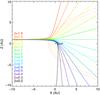 |
Fig. 1 Trajectories of interstellar dust coming into the solar system, having the same impact parameter b, but different β-values. The dotted lines show the (analytically calculated) β-cones. The dust is assumed to initially move parallel to the X-axis, for simplification. |
Assuming that the particle comes in parallel to the X-axis of a polar
coordinate frame where θ = 0 corresponds to the downstream dust
direction, its equation of motion written in polar coordinates is 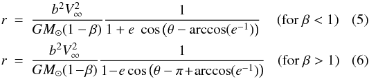 where
r is the heliocentric distance of the particle with respect to the
Sun, b the particle impact parameter, V∞
the speed of the particle at entrance to the solar sytem, and θ the
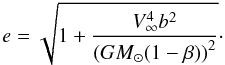
angle in polar coordinates corresponding to r. The eccentricity
e of the hyperbolic trajectory is equal to
where
r is the heliocentric distance of the particle with respect to the
Sun, b the particle impact parameter, V∞
the speed of the particle at entrance to the solar sytem, and θ the
angle in polar coordinates corresponding to r. The eccentricity
e of the hyperbolic trajectory is equal to
 (7)The radial and
tangential velocity components of the particles at position r is given
by
(7)The radial and
tangential velocity components of the particles at position r is given
by 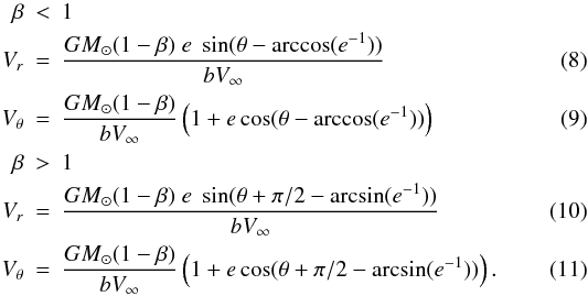 For
β < 1 all trajectories with equal impact
parameter b will cross each other at one point behind the Sun (focus)
and a region of enhanced dust densities will be generated by a beam of initially
parallel moving particles (Fig. 2). Since the
trajectories are rotationally symmetric about the beam axis, only trajectories in one
plane containing the beam axis are shown.
For
β < 1 all trajectories with equal impact
parameter b will cross each other at one point behind the Sun (focus)
and a region of enhanced dust densities will be generated by a beam of initially
parallel moving particles (Fig. 2). Since the
trajectories are rotationally symmetric about the beam axis, only trajectories in one
plane containing the beam axis are shown.
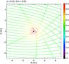 |
Fig. 2 Numerically calculated trajectories of particles with β = 0.5, but with different impact parameters b, in the ISD frame. The dust is concentrated downstream from the Sun. The particles accelerate near the Sun, and decelerate afterwards again to their original speed. The colorbar shows the scale of the absolute particle speed with a maximum of 50 km s-1. The particles are started at −50 AU from the Sun in 1997, and reach the region of the Sun about 9.5 years later. |
The focal distance df downstream from the Sun for particles
with equal β and b-values is given by 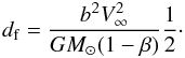 (12)For
β > 1 particles are deflected away from the
Sun and paraboloid-shaped regions are generated, which particles with a given
β-value cannot enter. These are the so-called
“β-cones” (dotted lines in Figs. 1
and 3).
(12)For
β > 1 particles are deflected away from the
Sun and paraboloid-shaped regions are generated, which particles with a given
β-value cannot enter. These are the so-called
“β-cones” (dotted lines in Figs. 1
and 3).
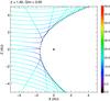 |
Fig. 3 Numerically calculated trajectories of particles with β = 1.6, but with different impact parameters b, in the ISD frame. The β-cone where particles with β > 1.6 cannot enter, is visible. Particles with β > 1 and no charge will decelerate near the Sun, and then accelerate again to their original speed. The colorbar shows the scale of the absolute particle speed with a maximum of 50 km s-1. The particles are started at −50 AU from the Sun in 1997, and reach the region of the Sun about 9.5 years later. |
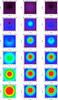 |
Fig. 4 Absolute differences in position, velocity, and direction, in “sliced” planes at different positions from the Sun along the X-axis of the ISD-frame. The difference between the case for β = 1, Q/m = 0, and β = 0.5, Q/m = 0 is shown. The red regions denote trajectory differences of more than 1 AU (left), velocity differences of more than 5 km s-1 (middle), and angular differences of more than 5 degrees (right). The plot illustrates in what extent the straight-line approximation can be used. |
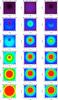 |
Fig. 5 Absolute differences in position, velocity, and direction, in “sliced” planes at different positions from the Sun along the X-axis of the ISD-frame. The difference between the case for β = 1, Q/m = 0, and β = 1.6, Q/m = 0 is shown. The red regions denote trajectory differences of more than 1 AU (left), velocity differences of more than 5 km s-1 (middle), and angular differences of more than 5 degrees (right). |
 |
Fig. 6 Cross-section of the trajectories for β = 0.5, through different YZ-planes in the ISD frame. The color denotes the particle speed in km s-1. The particles are started at 50 AU distance from the Sun. The speed of the particles is higher near the Sun. Farther away from the Sun, they slow down to their original starting speed. The density is enhanced downstream from the Sun. |
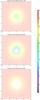 |
Fig. 7 Cross-section of the trajectories for β = 1.6, through different YZ-planes in the ISD frame. The color denotes the particle speed in km s-1. The particles are started at 50 AU distance from the Sun. The particles slow down near the Sun and accelerate again towards their original speed farther away from the Sun. The β-cone is visible. |
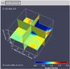 |
Fig. 8 Relative density map of ISD in the solar system up to 10 AU from the Sun, for particles with β = 1.6. The density is shown with respect to the undisturbed ISD density at infinity, and the color scale is limited to an upper relative density of 2. The β-cone for β = 1.6 is visible as a conically-shaped volume of depletion. |
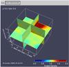 |
Fig. 9 Relative density map of ISD in the solar system up to 10 AU from the Sun, for particles with β = 0.5. The density is shown with respect to the undisturbed ISD density at infinity, and the color scale is limited to an upper relative density of 2. The relative density downstream of the Sun is enhanced thanks to the gravitational focusing. |
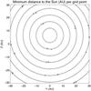 |
Fig. 10 Distance to the Sun during the closest approach for ISD particles with β = 0.5 and Q/m = 0, i.e. their closest distance to the Sun projected on a plane. The axes show the original position of the ISD particles in AU, in the ISD frame, while the numbers in the contour lines show their closest approach distances. The dotted lines are the reference case where β = 1 and Q/m = 0 (particles fly in straight lines, thus the dotted contour lines are circles). The contour lines for β = 0.5 are outside of the dotted contour lines, because the ISD is focused towards the Sun (so that a larger starting area is needed to investigate the ISD in an area of e.g. 10 AU around the Sun). |
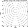 |
Fig. 11 Distance to the Sun during the closest approach for ISD particles with β = 1.6 and Q/m = 0, i.e. their closest distance to the Sun projected on a plane. The axes show the original position of the ISD particles in AU, in the ISD frame, while the numbers in the contour lines show their closest approach distances. The dotted lines are the reference case where β = 1 and Q/m = 0 (particles fly in straight lines, so the dotted contour lines are circles). The particles are “pushed away” by solar radiation pressure force, so less space is needed on the starting grid to investigate a certain area in the solar system. |
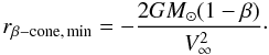
The polar equation of the exclusion zones is expressed as 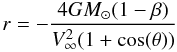 (13)(Altobelli 2004). The upstream apex distance of the
β-cone is given by
(13)(Altobelli 2004). The upstream apex distance of the
β-cone is given by
 (14)The deflections
from straight line trajectories are shown in Figs. 4 and 5 for particles with
β = 0.5 and β = 1.6, respectively. Upstream of the
Sun, the deflection (in distance and angle) and acceleration (in speed) are small, and
higher deflections are concentrated on trajectories close to the beam axis. Downstream
from the Sun, the scattering by solar gravitation and radiation pressure forces becomes
strong and straight line trajectories can no longer be used as proxies for interstellar
particle trajectories.
(14)The deflections
from straight line trajectories are shown in Figs. 4 and 5 for particles with
β = 0.5 and β = 1.6, respectively. Upstream of the
Sun, the deflection (in distance and angle) and acceleration (in speed) are small, and
higher deflections are concentrated on trajectories close to the beam axis. Downstream
from the Sun, the scattering by solar gravitation and radiation pressure forces becomes
strong and straight line trajectories can no longer be used as proxies for interstellar
particle trajectories.
The existence of the β-cones may help us restrict ISD particle properties by comparing the observations of the flux, density, direction, and speed of the particles, with the theoretically calculated values (Landgraf et al. 1999a). Such particle-dynamics studies can constrain the β-value of the ISD, and thereby providing some information about particle properties such as its composition or surface roughness. This study is referred to as β-spectroscopy (Altobelli 2004). However, the distribution of ISD in the heliosphere is much more complex than presented here, because it is modified by the Lorentz force due to the interaction of the IMF with the charged ISD particles. For β-spectroscopy, care has to be taken in the selection of the timeperiods of the observations, as well as the locations, to avoid mixing up the effects of eventual Lorentz forces with the β-cones.
2.1.2. Gravity and radiation pressure: densities
The density can be analytically expressed in polar coordinates as 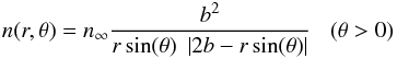 (15)where
 (16)(Landgraf et al. 1999b) with n the
local density, n∞ the undisturbed density of the ISD at
entrance to the solar system, b the impact parameter and
r and θ the polar coordinates of the dust particle,
with respect to the Sun. For β > 1 every
position outside the β-cone is reached by two different trajectories.
Since Eq. (15) only gives the
contribution to the number density of one solution, the contributions from the different
solutions that reach a point have to be added up to calculate the total number density
at a point (Landgraf et al. 1999b). The
distribution of ISD in the heliosphere due to solar gravity and radiation pressure force
is axisymmetric around the axis along the inflow vector of the dust. In Figs. 6 and 7 scatter
plots of the densities at different slices perpendicular to the particle beam are
displayed at different distances to the Sun. Downstream from the Sun the dust
concentrations along the beam axis are visible for the
β < 1 case. Close to the Sun, higher speeds
can be seen thanks to the solar acceleration (Fig. 6). In case of β > 1 (Fig. 7), the deceleration close to the Sun and the formation
of the β-cone becomes apparent with some density enhancements just
outside of the β-cone.
(16)(Landgraf et al. 1999b) with n the
local density, n∞ the undisturbed density of the ISD at
entrance to the solar system, b the impact parameter and
r and θ the polar coordinates of the dust particle,
with respect to the Sun. For β > 1 every
position outside the β-cone is reached by two different trajectories.
Since Eq. (15) only gives the
contribution to the number density of one solution, the contributions from the different
solutions that reach a point have to be added up to calculate the total number density
at a point (Landgraf et al. 1999b). The
distribution of ISD in the heliosphere due to solar gravity and radiation pressure force
is axisymmetric around the axis along the inflow vector of the dust. In Figs. 6 and 7 scatter
plots of the densities at different slices perpendicular to the particle beam are
displayed at different distances to the Sun. Downstream from the Sun the dust
concentrations along the beam axis are visible for the
β < 1 case. Close to the Sun, higher speeds
can be seen thanks to the solar acceleration (Fig. 6). In case of β > 1 (Fig. 7), the deceleration close to the Sun and the formation
of the β-cone becomes apparent with some density enhancements just
outside of the β-cone.
Besides the scatter plots shown in Figs. 6 and 7, 3-D density maps have also been calculated from numerically integrated trajectories. The β-cones are visible in the ISD density map of the solar system (see Fig. 8): for particles with β > 1, there is a depletion of particles downstream of the Sun. When β < 1 (see Fig. 9), the density of ISD downstream of the Sun increases (gravitational focusing of the Sun). Figures 8 and 9 are derived from the numerical trajectory simulations by counting the number of grains in the grid cells per time bin. They are drawn in the ecliptic reference frame. The density plots are fixed at one single observation time. The trajectory plots in this paper have a fixed starting time for the particles, but time evolves along the plotted trajectory. Since the ISD flow with only radiation pressure force and solar gravity is stationary, the density plots and trajectory plots will match each other. However, when Lorentz forces are taken into account, this is no longer the case.
2.1.3. Gravity and radiation pressure: closest distance to the Sun
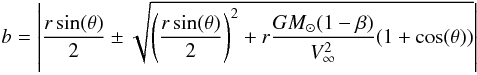
The closest approach distance to the Sun (perihelion distance
rCA) of the hyperbolic trajectories of interstellar grains
through the planetary system is given by 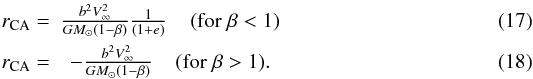 To
gain insight into the way that particles are spread or focused with respect to their
starting position, we plot the closest distance to the Sun of the ISD. The resulting
plot can be used to define the minimum size of the area where particles are started from
in the simulation. As an example, we plot the closest approaches for
particles with β = 0.5 and β = 1.6 in Figs. 10 and 11. The
plots are drawn in the ISD frame. The dotted lines are the closest approaches to the Sun
for a reference case with β = 1 and no charge, so the reference
particles move in straight lines towards the Sun. Their closest distance to the Sun is
equal to the distance of the particle on the starting grid to the center of the starting
grid (the contour lines in Fig. 10 are thus
circular). The offset in the Z direction is a result of the obliqueness of the incoming
dust vector with respect to the solar equatorial plane.
To
gain insight into the way that particles are spread or focused with respect to their
starting position, we plot the closest distance to the Sun of the ISD. The resulting
plot can be used to define the minimum size of the area where particles are started from
in the simulation. As an example, we plot the closest approaches for
particles with β = 0.5 and β = 1.6 in Figs. 10 and 11. The
plots are drawn in the ISD frame. The dotted lines are the closest approaches to the Sun
for a reference case with β = 1 and no charge, so the reference
particles move in straight lines towards the Sun. Their closest distance to the Sun is
equal to the distance of the particle on the starting grid to the center of the starting
grid (the contour lines in Fig. 10 are thus
circular). The offset in the Z direction is a result of the obliqueness of the incoming
dust vector with respect to the solar equatorial plane.
Particles with β < 1 are attracted near the Sun. Therefore, in order to get the total ISD density in a radius of 10 AU around the Sun, one needs to start the particles from a wider range than 10 AU in the start plane. How wide this range should be can be estimated from the plots. The plots show how much the particles are focused and defocused with respect to the Sun, in comparison with the case for straight trajectory lines.
2.2. Lorentz forces
ISD particles moving through the heliosphere collect ions and electrons from the ambient
solar wind plasma. They also emit electrons, mainly owing to the photo-ionionization
effect of the solar UV radiation. The electron fluxes are much higher than the ion fluxes,
and the amount of electrons emitted through the photo-ionization effect is more than
electron collection through the solar wind plasma. Therefore the particle will get a
positive charge, which brings the emission and collection currents into equilibrium. Since
the solar UV radiation intensity and the solar wind plasma density both decrease
quadratically with increasing distance to the Sun, this charge stays in equilibrium (Horányi 1996). It has been estimated that the surface
potential on graphite grains at 1 AU from the Sun is between +0.5 V and +6 V (depending on
solar wind conditions), while the surface potential on silicate grains at 1 AU is about
+4 V and +14 V (Mukai 1981). With changing solar
wind conditions, the potential of the grains will fluctuate too, but these fluctuations
are only small and temporary. For the ISD simulations, we assume spherical unfluffy
grains, with an equilibrium potential of +5V, which is compatible with the Cassini
measurements (Kempf et al. 2004) of
charged grains. These measurements confirm the theoretical predictions of the charges on
ISD grains. The net charge on the dust grain is then 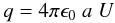 (19)where
ϵ0 is the electric permittivity of the vacuum
(8.85 × 10⁻¹² F/m), a the radius of the grain, and
U the surface potential. Assuming a spherical grain with density
ρ and mass m, the charge to mass ratio becomes
(19)where
ϵ0 is the electric permittivity of the vacuum
(8.85 × 10⁻¹² F/m), a the radius of the grain, and
U the surface potential. Assuming a spherical grain with density
ρ and mass m, the charge to mass ratio becomes
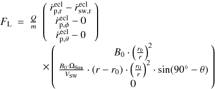
 (20)When the charged
particles move through the IMF, they experience Lorentz forces. The Lorentz force exerted
on ISD depends on the particles charge to mass ratio
(Q/m), its velocity with respect to
the solar wind velocity (ṙp,sw)
and on the field strength of the IMF (Bsw) at the
location of the particle. The equation of motion of the ISD becomes
(20)When the charged
particles move through the IMF, they experience Lorentz forces. The Lorentz force exerted
on ISD depends on the particles charge to mass ratio
(Q/m), its velocity with respect to
the solar wind velocity (ṙp,sw)
and on the field strength of the IMF (Bsw) at the
location of the particle. The equation of motion of the ISD becomes
 (21)At large distances
from the Sun, the main IMF component is the azimuthal component of the IMF (see
Sect. 2.3), so the main effect of the Lorentz force
is to deflect the ISD particles towards or away from the solar equatorial plane (Morfill & Grün 1979; Gustafson & Misconi 1979). Whether particles will be focused or
defocused depends on the phase of the solar cycle. The Lorentz forces can narrow down the
β-cones, or the opposite, enhance the β-cones. The
importance of the Lorentz force with respect to solar gravity increases linearly with the
distance to the Sun:
(21)At large distances
from the Sun, the main IMF component is the azimuthal component of the IMF (see
Sect. 2.3), so the main effect of the Lorentz force
is to deflect the ISD particles towards or away from the solar equatorial plane (Morfill & Grün 1979; Gustafson & Misconi 1979). Whether particles will be focused or
defocused depends on the phase of the solar cycle. The Lorentz forces can narrow down the
β-cones, or the opposite, enhance the β-cones. The
importance of the Lorentz force with respect to solar gravity increases linearly with the
distance to the Sun:  (22)Only closer to
the Sun (<~2 AU) will the radial component of the magnetic
field play a larger role and the Lorentz force and gravity are not linearly related, but
relate as
(22)Only closer to
the Sun (<~2 AU) will the radial component of the magnetic
field play a larger role and the Lorentz force and gravity are not linearly related, but
relate as
 (23)where
r is given in AU; i.e., for distances less than 1 AU,
FL ∝ FG. At 1 AU,
FL = 1.4FG and at 2 AU,
FL = 2.23FG. The effects of the
Lorentz forces are discussed in detail in Sect. 4.
(23)where
r is given in AU; i.e., for distances less than 1 AU,
FL ∝ FG. At 1 AU,
FL = 1.4FG and at 2 AU,
FL = 2.23FG. The effects of the
Lorentz forces are discussed in detail in Sect. 4.
Figure 12 gives an overview of the relative
importance of the Lorentz force, solar gravitation, and solar radiation pressure force,
from Landgraf (1998). Solar gravitation and solar
radiation pressure force are combined into one “effective gravitation” term (see
Eq. (3)). The ratio of the Lorentz force
to the effective gravitation is given as function of particle size a and
distance to the Sun r. Assumed is a β-particle-size
dependency (β-curve) for astronomical silicates,
from Gustafson (1994). The ratio of gravity and
radiation pressure force is 1 for particles of sizes of approximately
0.1 μm and 0.35 μm, which can be seen in Fig. 12:
gravity and radiation pressure cancel, and the Lorentz force takes over entirely. The plot
shows 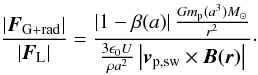 (24)
(24)
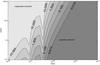 |
Fig. 12 Ratio of Lorentz force to “effective gravitation” for several particle sizes and at different distances from the Sun, from Landgraf (1998). |
2.3. Modeling the interplanetary magnetic field
The Sun expels a vast amount of plasma into the heliosphere: the solar wind. This plasma,
streaming radially outward, convects the magnetic field of the Sun along on its way into
interplanetary space. Because the Sun is rotating, the field lines are winding up, forming
a spiral – the so-called Parker spiral – parallel to the solar equatorial
plane (Parker 1958). In the Parker model, the
radial component of the IMF field strength Br
decreases with the square of the distance to the Sun, while the azimuthal
component Bφ decreases only linearly. The
equations describing the IMF are 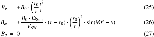 (Parker 1958) where r,
φ, and θ are the radial distance, the longitude and
latitude of the position of the dust particle in the solar wind, respectively (in a
coordinate system that has its XY-plane in the solar equatorial plane).
In this model we assume one rotation every ≃25.38 days (sidereal period) for both the
poles and the equator of the Sun. Here, B0 = 2300 nT is the
magnetic field strength at a reference distance r0 from the
Sun, which is the distance from the center of the Sun where the field lines are assumed to
go radially outward. The reference distance in the simulation model is 10 solar
radii (Parker 1958). The field strength at the
Earth is 5 nT.
(Parker 1958) where r,
φ, and θ are the radial distance, the longitude and
latitude of the position of the dust particle in the solar wind, respectively (in a
coordinate system that has its XY-plane in the solar equatorial plane).
In this model we assume one rotation every ≃25.38 days (sidereal period) for both the
poles and the equator of the Sun. Here, B0 = 2300 nT is the
magnetic field strength at a reference distance r0 from the
Sun, which is the distance from the center of the Sun where the field lines are assumed to
go radially outward. The reference distance in the simulation model is 10 solar
radii (Parker 1958). The field strength at the
Earth is 5 nT.
Equations (25) and (26) show that, at large distances, the IMF is
dominated by its azimuthal component. During solar minimum, the solar wind speed varies
between about 400 km s-1 at the solar equator, and 800 km s-1 at
higher latitudes. At solar maximum, the speeds are more moderate and more uniformly
divided over the Sun. For the model, we adapted a constant solar wind speed at all
latitudes of 400 km s-1. Since the azimuthal component of the IMF is inversely
linear to the solar wind speed, and since we assume that the solar wind blows radially
outward of the Sun, the Lorentz force becomes independent of the solar wind speed (Gustafson & Misconi 1979)1:
 (28)with
FL the Lorentz force,
(28)with
FL the Lorentz force,
 the
charge to mass ratio of the particle,
the
charge to mass ratio of the particle,  the radial velocity of the particle in the ecliptic coordinate frame,
 the radial solar wind velocity in the ecliptic coordinate frame, and
 and
and  are the azimuthal and elevation components of the particle velocity in the ecliptic
coordinate frame.
are the azimuthal and elevation components of the particle velocity in the ecliptic
coordinate frame.
The solar magnetic field is modeled as a dipole, where the magnetic field lines extend into interplanetary space. The Parker model determines the direction (shape) and strength of the IMF, but the polarity of the field (positive when field lines are directed “outward” from the Sun, negative when they are directed “inward” towards the Sun) depends on the position of the dust particle with respect to the Heliospheric Current Sheet (HCS). The HCS divides the regions of positive polarity from the regions of negative polarity and is modeled as a flat sheet in our simulations. The modeled HCS is aligned with the solar equatorial plane during solar minimum, while at solar maximum, the “sheet” is rotated by 90° and is aligned with the solar rotation axis. As a result, the modeled HCS turns 360°, at a steady rate of 22 years around a reference axis2 in the solar equatorial plane. In the meantime, the HCS turns around the solar rotation axis in 25.38 days. At solar maximum, an observer in the solar equatorial plane, would thus see 50% of the time a negative polarity, and the other 50% of the time a positive polarity. Because the equatorial plane of the Sun is tilted with respect to the ecliptic frame, an observer at the Earth will observe two “sectors” of opposite polarity during one solar rotation. In reality, the HCS is not flat but slightly warped at solar minimum (hence, an observer at the Earth would observe more (e.g. four) sectors of opposite polarity during one solar rotation), and during solar maximum there is no longer any clear dipolar structure. However, the flat sheet model is a good approximation for our purposes.
The field polarity in the model is thus determined by the phase of the solar cycle and the latitude and longitude of the observer. Three different models of the IMF are included in the simulations, and the choice of model to use depends on the particle location:
-
1.
The HCS is modeled to turn at a steady rate of 22 years around a reference axis in the solar equatorial plane, and the magnetic field strength at the location of a dust particle is averaged over one solar rotation. The solar cycle reference time, t0, is July 1974, where the Sun was modeled to be in solar minimum (HCS is aligned with solar equatorial plane, the northern solar hemisphere has a positive polarity, and the southern solar hemisphere has negative polarity. This model can be used when the speed of the particles is not too fast with respect to the rotation of the Sun, which is the case for ISD. Since we average the IMF over one solar rotation, the results are also only applicable to situations where shorter timescales are unimportant, i.e. outside 1–2 AU. Landgraf (2000) has used these assumptions for the IMF modeling.
-
2.
The HCS is modeled to turn at a steady rate of 22 years around a reference axis in the solar equatorial plane, and the true local magnetic field is calculated at each location of the dust particles, instead of averaging out over one solar rotation. This model is useful for calculations closer to the Sun, for high time-resolution calculations, or for fast particles like nanodust with velocities of 100 to 200 km s-1.
-
3.
The HCS angle is determined by the modeling from solar data between 1976 and 2009 from the Wilcox Solar Observatory (Hoeksema 2011). The HCS angle is thus slightly different from the angles of the steady-state rotation of the previously described model. The magnetic field is averaged over one solar rotation. The HCS angle is shown in Fig. 13, from 1976 until 2009.
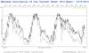 |
Fig. 13 Computed tilt of the heliospheric current sheet, from Solar Wilcox Observatory (Hoeksema 2011). |
An overview of the modeled solar cycle.
2.4. Particle properties, β and Q/m
The study of the ISD dynamics is governed by three parameters that determine the path of the dust through the solar system: β, Q/m, and time. The β determines the solar radiation pressure force to gravity ratio, which reduces the number of parameters from four to the stated three. The ratio Q/m and time (related to the phase of the solar cycle) determine the Lorentz force. Both β and Q/m are fairly unknown, since we do not know the exact composition, mineralogy, structure, and material properties of ISD. Realistic boundaries are set for these parameters through previous laboratory studies of dust and astronomical observations of the ISD (see Draine 2009; and Sect. 2.4.1). We perform the dust simulations for a wide range of parameters. These are summarized in Sect. 2.4.3.
2.4.1. Discussion of parameter β
Dust particles are characterized by their mass, size, composition, and shape which affect the dynamics of interstellar grains within the solar system. All of these parameters are not, or only weakly, constrained for local interstellar grains. Astronomical observations of UV extinction and infrared emissions indicate carbonaceous particles (polycyclic aromatic hydrocarbons, PAHs, or graphite grains) and amorphous silicate grains. Analysis of in-situ Ulysses data by Landgraf et al. (1999a) suggests absorbing silicates for the particles penetrating the planetary system. Compositional analyses of collected interstellar grains by the Stardust mission are not available yet.
The interactions of dust with solar radiation are determined by the optical properties
of the particle that are a function of the particle parameters size, composition, and
shape. In Eq. (4) the cross section
Ap and the efficiency factor
Qpr for radiation pressure describe this interaction. For
particles ≫ 1μm, Qpr is roughly constant
and depends only on the absorption efficiency of the particle material at visible
wavelengths. Since absorption occurs at the surface of the particles, surface
composition is important rather than bulk composition, which may be different. The size
dependency of β is proportional
to  .
.
For particles <1 μm, scattering of sunlight also becomes important. The scattering efficiency can be calculated for spherical particles by Mie-scattering theory and for particles that are much smaller than the wavelength, Rayleigh scattering can be applied (Burns et al. 1979). For nonspherical particles, elaborate scattering algorithms have often been applied, and even laboratory simulations are used to obtain relevant Qpr values for determining relevant β values (see Gustafson et al. 2001, for a review). Kimura & Mann (1999) calculated β-curves for fluffy carbon and silicate particles (Fig. 14). Very fluffy fractal particles are not likely to survive the harsh interstellar environment for long; therefore, we consider compact particles to be nominal.
The β-curve for astronomical silicates (Gustafson 1994) is adapted to the Ulysses observations to have a maximum β-value of βmax = 1.6 (Landgraf et al. 1999a). This curve (see Fig. 15), is used to produce five nominal cases as defined in Table 3, which illustrates a few realistic sets of parameters and particle sizes. Four of them are indicated in Fig. 15. However, since the properties of interstellar particles and their respective β-values are not strongly constrained, we simulated dust trajectories for a wide range of β and Q/m values instead of following only one curve.
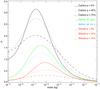 |
Fig. 14 β-curves from Kimura & Mann (1999) showing the influence of porosity on the β-value of the dust, namely a flattening of the curve. |
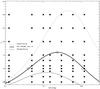 |
Fig. 15 Overview of the simulations performed with various β and Q/m values. All simulations are done between 2010 and 2030, where densities and fluxes are binned per 100 days, and in a region of the solar system in a box of 22 AU around the Sun. The crosses denote these simulations (β and Q/m range), while the curves are three examples of β-curves: two from Kimura & Mann (1999) and one “adapted” astronomical silicates curve (Gustafson 1994). The β-curves relate the β-parameter of a material to its size. The sizes are consequently converted in corresponding charge-to-mass ratio, assuming a surface potential of +5 V and the material density according to the corresponding material (see Eq. (20)). The diamonds on the adapted astronomical silicates curve are 4 out of the 5 parameter combinations given in Table 3, that illustrate “realistic” sets of parameters for one material and their relation to particle size. |
The β and Q/m values used for the plots in this document.
2.4.2. Discussion of parameter Q/m
The electrical surface potential on dust particles in interplanetary space depends mostly on the ambient solar wind parameters, density and flux, whereas the solar UV flux, hence the photo electron emission, are not that variable. Photo electron emission yields have been determined experimentally for dielectric and absorbing materials (Feuerbacher & Fitton 1972). Dielectric materials have an electron yield of about 0.1 times the yield of absorbing materials. Since the grain potential is determined by the balance of plasma and photo electron currents, the equilibrium potential of dielectric grains is only slightly reduced. For both materials we use a surface potential of +5 V, which is compatible with measurements of dust charges on interplanetary particles (Kempf et al. 2004). There is a dependence on the shape of the particle. Elongated or flat particles carry higher charges than spherical particles at the same surface potential (Hill & Mendis 1981). Very fluffy particles carry even higher charges than spherical particles (Auer et al. 2007), however, these particles are also more susceptible to electrostatic disruption. We conclude that the charge on interstellar grains deviates by less than a factor 2 from that of a spherical particle.
2.4.3. Overview of used β and Q/m-values
State-of-the-art in-situ dust telescopes (Srama et al. 2004b; Sternovsky et al. 2010) will provide the magnitude and direction of the ISD flux at various times and positions in the planetary system, in addition to the masses and speeds of individual particles. Recent measurements of interstellar grains by the dust detector onboard Ulysses (Krüger et al. 2007) provided the magnitude, direction, and mass distribution of the ISD flux between Earth’s and Jupiter’s orbits. To interpret these measurements in terms of optical and physical properties of interstellar grains, we calculated dust trajectories through the planetary system for a wide range of β and Q/m values, along with the starting times over a complete solar cycle of 22 years (Fig. 15). Any measurement of the interstellar particle flux (direction, speed) of a given particle mass at a given position and time can be compared with possible trajectories that have the similar characteristics. Therefore, a set of measurements at different positions, times, and/or particle masses will constrain the β and Q/m values for these particles, so it will constrain the physical and compositional properties of interstellar grains. Previously Landgraf et al. (1999a) succeeded at such an analysis using the effect of β on the mass distribution. Figure 15 gives an overview of the parameters of the performed simulations.
3. Simulation tool
Monte Carlo simulations are performed for the trajectories of individual ISD particles through the heliosphere using the modeling as described in Sects. 2 and 2.3. Hereby, the starting conditions for these trajectories were varied arbitrarily in starting position and time. From these trajectories we derived ISD density maps and fluxes throughout the solar system, by counting the amount of particles per grid cell and per time bin. The dust dynamics follow the description of Sect. 2, which are largely the same assumptions (except for the β and Q/m parameters) as in Landgraf (1998, 2000). The Lorentz forces depend on the IMF. Three models of the IMF are implemented, whose use depends on the speed for the dust and the distance to the Sun of the region we are interested in.
The simulations contain two possible coordinate systems: the J2000 ecliptic frame, and the “ISD simulation frame”. The frames are depicted in Fig. 16. Ecliptic frame. In the ecliptic frame, the dust flow is directed towards 79° longitude, −8° latitude (downstream) (Frisch et al. 1999). The flow is thus roughly along the Y-axis (11° offset in the XY-plane, −8° offset in the YZ-plane). ISD frame. The Z-axis of the ISD frame is equal to the solar rotation axis, and the XY-plane is equal to the solar equatorial plane. The X-axis is perpendicular to the Z-axis, and the XZ-plane is defined by the direction of the velocity vector of the dust. In the XZ-plane, the dust flows mainly along the X-axis, with an offset of about 7.5° in the −Z direction. The Y-component of the initial dust velocity vector is zero in this frame.
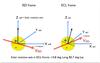 |
Fig. 16 The ISD frame and the ECL frame. |
3.1. Assumptions of the model
Several assumptions were made for modeling the dust dynamics of ISD in the solar system.
-
the solar wind speed is constant;
-
the potential of the dust grain is constant with the influence of solar wind speed and density variations. The influence of grain shape/fractality is not considered;
-
differential rotation of the Sun is not taken into account, but is assumed to have nearly no influence anyway;
-
no assumptions are made yet about the incoming mass distribution of the particles. All results are relative to the density, velocity and flux before entering the solar system;
-
filtering at the heliopause is not yet taken into account;
-
the incoming submicrometer sized grain flux is modeled as monodirectional and homogeneous, since it is coupled to the gas in the LIC.
 |
Fig. 17 3D-representation of a “sheet” of particle trajectories with β = 1.0 and Q/m = 0.5 C/kg, during the focusing phase of the solar cycle. The start year is 2000. The “sheet” of particles is started along the Y-axis of the ISD frame. The focusing towards the solar ecliptic plane is visible, but at the same time there is a “defocusing” in the XY-plane (see projection), downstream of the Sun. The color denotes the particle speed in km s-1. |
4. Results and discussion
The influence of the solar gravity and radiation pressure force on the ISD trajectories were discussed in detail in Sect. 2.1 and the Lorentz force was introduced in Sect. 2.2. In this section we discuss the effect of the Lorentz forces on the particle trajectories and densities.
Because we averaged the solar wind magnetic field over one solar rotation (25.38 days), our simulation results are only appropriate for larger distances to the Sun, e.g. >2 AU. Any conclusions concerning the interstellar flux at 1 AU should be taken with caution. A subsequent paper will deal with this situation by analyzing the results, by using a finer resolution and the unaveraged solar magnetic field model. All particles are started at a distance of about 50 AU from the Sun. For β = 1, Q/m = 0, they would reach the Sun about nine years later.
4.1. Hypothetical dust flow for Lorentz force “only” (β = 1)
To show the influence of the Lorentz force clearly, we studied the trajectories for a particle with β = 1 and Q/m = 0.5 C/kg, and to understand the effects of the Lorentz force on ISD trajectories, we varied Q/m up to 12 C/kg, keeping β = 1.
4.1.1. Q/m = 0.5 C/kg
The special configuration of the interstellar flow (close to the solar rotation equator) and the dominant azimuthal component of the magnetic field at low latitudes (in the outer solar system), are the reasons that Lorentz force acts mostly normal to the equatorial plane. The axial symmetry of the radiation-pressure-only case is therefore broken. We demonstrate this effect by showing dust trajectories in two sheets: one close to and parallel to the solar rotational equator (Figs. 17, 18)3 and another sheet perpendicular to the equatorial plane (Figs. 19–22). The dominant deflection of trajectories occurs close to the Sun in a direction perpendicular to the equatorial plane. The varying magnetic field configuration during the 22-year solar cycle has a focusing and defocusing effect roughly 11 years later (Morfill & Grün 1979). The maximum defocusing effect occurs for particles launched 50 AU from the Sun in ~1990 (Fig. 19) followed by almost no deflection in 1995 (Fig. 20) while the maximum focusing effect occurs for particles launched in ~2000 (Fig. 21). For particles launched in 2006, already significant defocusing can be observed when they reach the region of the Sun. In the focusing period, particles get decelerated by the solar wind magnetic field, while their trajectories are bent towards the current sheet. The opposite occurs during the defocusing period when the particles are accelerated away from the current sheet.
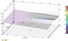 |
Fig. 18 3D-representation of a “sheet” of particle trajectories with β = 1.0 and Q/m = 0.5 C/kg, during the defocusing phase of the solar cycle. The start year is 1990. The “sheet” of particles is started along the Y-axis of the ISD frame. While the particles are defocused with respect to the solar equatorial plane, they are focused in the XY-plane (see projection) downstream of the Sun. |
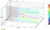 |
Fig. 19 3D-representation of a “sheet” of particle trajectories with β = 1.0 and Q/m = 0.5 C/kg during the defocusing phase of the solar cycle. The start year is 1990. The particles are started in a “sheet” along the Z-axis to illustrate the defocusing effect of the Lorentz force with respect to the solar equator. In general, during the defocusing phase of the solar cycle, the particles are accelerated in the neighborhood of the Sun. Since β = 1, we only see the influence of the Lorentz forces (not the radiation pressure force or gravity). |
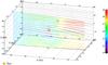 |
Fig. 20 β = 1.0, Q/m = 0.5 C/kg. Start year is 1995. The phase of the solar cycle is just after the solar maximum from the defocusing to focusing cycle, resulting in only moderate deflections. |
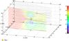 |
Fig. 21 3D-representation of a “sheet” of particle trajectories with β = 1.0 and Q/m = 0.5 C/kg during the focusing phase of the solar cycle. The start year is 2000. The particles are started in a “sheet” along the Z-axis to illustrate the focusing effect of the Lorentz force with respect to the solar equator. In general, during the focusing phase of the solar cycle, the particles are decelerated in the neighborhood of the Sun. Since β = 1, we only see the influence of the Lorentz forces (not the radiation pressure force or gravity). |
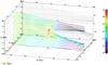 |
Fig. 22 β = 1.0, Q/m = 0.5 C/kg. Start year is 2006. The phase of the solar cycle is just after the solar maximum from the focusing to defocusing cycle, resulting in only moderate deflections. |
While upstream at Kuiper belt distance (>30 AU), the ISD trajectories can be considered straight lines (Figs. 23, 24), strong deflections, both in distance, angle, and modifications in speed already occur at the (upstream) distance of Saturn (10 AU). At Jupiter’s distance (5 AU), only trajectories close to the solar equatorial plane can be approximated with straight lines. The solar equatorial plane is tilted with ~7° from the ecliptic plane, so at the distance of Saturn, this is as much as 1.2 AU above or below the ecliptic plane.
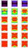 |
Fig. 23 Absolute differences in position (red = difference d > 1 AU), velocity (d > 5 km s-1) and direction (d > 5°) in different “sliced” planes at different distances from the Sun. The case for β = 1, Q/m = 0.5 C/kg is compared to the straight-line approximation (β = 1, Q/m = 0). Start year is 1990 at −50 AU from the Sun. The phase of the solar cycle is the defocusing phase. |
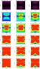 |
Fig. 24 Absolute differences in position (red color = difference d > 1 AU), velocity (d > 5 km s-1) and direction (d > 5°) in different “sliced” planes at different distances from the Sun. The case for β = 1, Q/m = 0.5 C/kg is compared to the straight-line approximation (β = 1, Q/m = 0). Start year is 2000 at −50 AU from the Sun. The phase of the solar cycle is the focusing phase. |
The “closest approach” distances of trajectories (Figs. 25, 26) show the effect of focusing and defocusing due to the Lorentz force. In Fig. 25, the areas where particles reach a certain minimum distance to the Sun (solid lines) is extended in the polar direction indicating that particles that were initially farther away from the beam axis get closer to the Sun than particles on straight line trajectories. So in Fig. 25, the particles are focused towards the Sun along the Z-direction. In the Y-direction, there is little or no focusing or defocusing at the closest distance to the Sun, with respect to the straight line case (β = 1, Q/m = 0). In defocusing periods, the range where particles reach a certain minimum distance is shrunk in the polar direction (Fig. 26). The particles are defocused from the solar equatorial plane. In the Y-direction, there is little or no focusing or defocusing at the time the particle is closest to the Sun, with respect to the straight line case (β = 1, Q/m = 0).
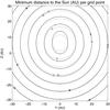 |
Fig. 25 Closest distances of the particles to the Sun, projected on a plane, during their trajectory for β = 1, Q/m = 0.5 C/kg, during the focusing phase of the solar cycle. The axes show the original position of the ISD particles in AU, in the ISD frame, while the numbers in the contour lines show their closest approach distances. The dotted lines are the reference case where β = 1 and Q/m = 0. (Particles fly in straight lines, thus the dotted contour lines are circles.) |
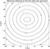 |
Fig. 26 Closest distances of the particles to the Sun, projected on a plane, during their trajectory for β = 1, Q/m = 0.5 C/kg, during the defocusing phase of the solar cycle. The axes show the original position of the ISD particles in AU, in the ISD frame, while the numbers in the contour lines show their closest approach distances. The dotted lines are the reference case where β = 1 and Q/m = 0. (Particles fly in straight lines, thus the dotted contour lines are circles.) |
The dust density enhancements and depletions near the solar equator are best seen in the scatter plots (Figs. 27 and 28). Although density variations can be seen upstream of the Sun (− 5 AU), the effects are strongest downstream of the Sun. While the dust densities decrease close to the solar equator during the defocusing period, density enhancements at higher latitudes can be observed. Also the deceleration during focusing periods and acceleration during defocusing periods are visible.
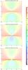 |
Fig. 27 Several cross-sections through the trajectories at different distances from the Sun (− 5 AU, 0 AU, and 5 AU) in the ISD-frame. The trajectories shown are for particles with β = 1.0 and Q/m = 0.5, started in 2000 at −50 AU from the Sun. The focusing effect of the Lorentz force is visible. This plot is directly comparable to the two corresponding trajectory plots (Figs. 17 and 21). |
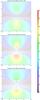 |
Fig. 28 Several cross-sections through the trajectories at different distances from the Sun (− 5 AU, 0 AU, and 5 AU) in the ISD-frame. The trajectories shown are for particles with β = 1.0 and Q/m = 0.5, started in 1990 at −50 AU from the Sun. The defocusing effect of the Lorentz force is visible and results in a void downstream from the Sun. Several AU above the solar ecliptic plane, two regions of higher ISD particle concentrations are visible. This plot is directly comparable with Figs. 18 and 19. |
The ISD densities inside a cube of 22 AU width are displayed in Figs. 29 and 30. At 50 AU from the Sun, dust particles were continuously launched at random times within a time range of about 45 years. The dust densities in the inner solar system at different times from 1996 to 2018 show strong density variations. From 1996 to about 2006 the dust densities were generally lower than the initial densities (Fig. 29), whereas the densities were higher afterwards (Fig. 30). The solar minimum of the defocusing cycle is in mid-1996. The maximum effect of this on the density is about three years later. Solar maximum is in 2002 and the solar minimum of the focusing cycle is in mid-2007 (see Table 2). Again the effect of this on the density occurs about three years later in 2010. This time lag of several years is caused by the long travel time (about 9–10 years) in the region where the solar wind magnetic field significantly affects the dust trajectories. The focusing and defocusing effects are most prominent near the ecliptic, while the dust densities display a more complex variation at higher latitudes.
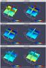 |
Fig. 29 Variation in relative densities in the solar system, due to the Lorentz force (β = 1, Q/m = 0.5 C/kg). Observing times are from left to right and top to bottom: 1996, 1998, 2000, 2002, 2004, 2006. The solar minimum of the defocusing cycle is in mid-1996. The maximum effect of this on the density is about 3 years later. Solar maximum is in 2002, and the solar minimum of the focusing cycle is in mid-2007. |
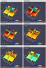 |
Fig. 30 Variation in relative densities in the solar system, due to the Lorentz force (β = 1, Q/m = 0.5 C/kg). Observing times are from left to right and and top to bottom: 2008, 2010, 2012, 2014, 2016, 2018. The solar minimum of the focusing cycle is in mid-2007. The maximum effect of this on the density is about 3 years later. Solar maximum is in 2013, and the solar minimum of the next defocusing cycle is in mid-2018. |
4.1.2. Q/m = 1.5 C/kg
Trajectories of dust particles with Q/m = 1.5 C/kg are strongly scattered by the solar wind magnetic field (Figs. 31, 32). Again the strongest deflection occurs in the vertical sheet of trajectories. A strong defocusing effect can be observed in 1990, whereas in 2000 particles are strongly bent towards the equatorial plane. Some trajectories that approach close to the Sun during the focusing cycle even cross the equatorial plane in front of the Sun. Again particles’ speed are accelerated and decelerated at even stronger levels than at lower Q/m values. Only at Kuiper belt distances is the deflection upstream from the Sun is small and the trajectory can be approximated by straight lines. Everywhere else trajectories have to be calculated more accurately.
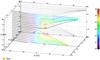 |
Fig. 31 β = 1.0, Q/m = 1.5 C/kg. Start year 1990, at −50 AU from the Sun. The main effect is defocusing. |
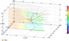 |
Fig. 32 β = 1, Q/m = 1.5 C/kg. Start year 2000, at −50 AU from the Sun. The main effect is focusing, particles are even already clearly focused upstream of the Sun. |
During the focusing cycle dust densities are strongly enhanced 5 AU upstream of the Sun in the equatorial plane (Fig. 33). Close to the Sun and downstream from the Sun in the central part of the beam, the dust slows down and the dust densities decrease, while the enhancements move outward in the equatorial plane. During the defocusing cycle, the dust densities are strongly depleted near the equatorial plane whereas at high latitudes dust concentrations develop downstream from the Sun (Fig. 34).
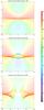 |
Fig. 33 Cross-section of the trajectories during the focusing phase of the solar cycle. Start year was 2000, β = 1, Q/m = 1.5 C/kg. |
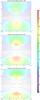 |
Fig. 34 Cross-section of the trajectories during the defocusing phase of the solar cycle. Start year was 1990, β = 1, Q/m = 1.5 C/kg. |
The contrast between dust concentrations during the focusing cycle and density depletions during defocusing periods (Figs. 35, 36) becomes even stronger than for Q/m = 0.5. The depletions are stronger and the concentrations are higher.
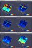 |
Fig. 35 Variation in relative densities in the solar system, due to the Lorentz force (β = 1, Q/m = 1.5 C/kg). Observing times are from left to right and top to bottom: 1996, 1998, 2000, 2002, 2004, 2006. The solar minimum of the defocusing cycle is in mid-1996. The maximum effect of this on the density is about 3 years later. Solar maximum is in 2002, and the solar minimum of the focusing cycle is in mid-2007. |
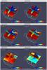 |
Fig. 36 Variation in relative densities in the solar system, due to the Lorentz force (β = 1, Q/m = 1.5 C/kg). Observing times are from left to right and top to bottom: 2008, 2010, 2012, 2014, 2016, 2018. The solar minimum of the focusing cycle is in mid-2007. The maximum effect of this on the density is about 3 years later. Solar maximum is in 2013, and the solar minimum of the next defocusing cycle is in mid-2018. |
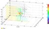 |
Fig. 37 β = 1.0, Q/m = 3 C/kg. Start year 2000, at −50 AU of the Sun. The particles are strongly focused, even upstream from the Sun. Particles with a low impact factor are reflected, while particles with an impact factor greater than about 20 AU are seen to pass downstream from the Sun. |
4.1.3. Q/m = 3 to 12 C/kg
Trajectories of interstellar grains of 1.5 C/kg during the focusing cycle (Fig. 32) already displayed significant deflection upstream of the Sun. To study this effect we increased Q/m to 3 C/kg (Fig. 37). Trajectories in the horizontal sheet displayed minimum deflections, whereas trajectories with impact parameters <20 AU in the vertical sheet were completely reflected upstream of the Sun. Only trajectories with impact parameters >20 AU were able to pass the Sun.
Even more bizarre are trajectories of Q/m = 12 C/kg particles in the vertical sheet (Fig. 38). Here, all particles with impact parameters <30 AU are reflected onto trajectories with high elevation angles. However, trajectories with impact parameters <10 AU can reach close proximity to the Sun before they are reflected. Their motion resembles trajectories of charged particles bouncing back in the high field region of a magnetic mirror. The motion of dust particles towards the Sun is coupled with a strong deceleration, while particles retreating from the Sun are initially strongly accelerated. During the defocusing cycle they are strongly diverted away from the Sun but maintain their general downstream motion (Fig. 39). During this deflection the particles are strongly accelerated and reach speeds twice their initial speed. At high latitudes (10–15 AU above the equatorial plane), higher concentrations of particles are found during defocusing periods.
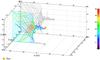 |
Fig. 38 β = 1.0, Q/m = 12 C/kg. Start year 2000, at −50 AU of the Sun. The particles are reflected upstream of the Sun and accelerated to high speeds. Particles with a low impact factor get far into the inner solar system (hypothetically assumed they are not already filtered at the heliosphere) and are reflected upstream of the Sun. |
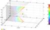 |
Fig. 39 β = 1.0, Q/m = 12 C/kg. Start year 1990, at −50 AU from the Sun. The particles are strongly deflected away from the solar equatorial plane, and are accelerated to high speeds on their way out of the solar system. |
The densities of these particles in the inner planetary system are rather low (Figs. 40, 41). These particles cannot reach the inner planetary system most of the 22-year solar cycle. Only for a short period after the maximum focusing are configuration particles concentrated close to the ecliptic plane. Upstream at 10 AU these particles are more abundant.
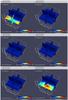 |
Fig. 40 Variation in relative densities in the solar system, due to the Lorentz force
(β = 1, |

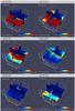 |
Fig. 41 Variation in relative densities in the solar system, due to the Lorentz force
(β = 1, |
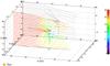 |
Fig. 42 β = 1.5, Q/m = 1.5 C/kg. Start year 2000, at −50 AU from the Sun. The particles are focused towards the solar equatorial plane and for low-impact parameters they are reflected upstream of the Sun. The effect is a bit stronger than without radiation pressure force (compare with Fig. 32). |
4.2. Flow of nominal ISD particles (β = 1.5, Q/m = 1.5 C/kg)
In the previous sections we studied the trajectories for hypothetical particles with radiation pressure alone (Sect. 2.1.1) and Lorentz force “only” (Sect. 4.1). However, some of these discussions apply to the flow of real interstellar grains. In Table 4, the β and Q/m values are given for nominal interstellar particles close to a hypothetical β-curve for astronomical silicates with βmax = 1.6. The table also lists the sections in this paper where the results for the particles with these values are discussed.
β and Q/m values for nominal interstellar particles close to the hypothetical β-curve for astronomical silicates with βmax = 1.6.
For 0.5 μm particles (Q/m = 0.2 C/kg), the Lorentz force effects are considered to be small, so the case discussed in Sect. 2.1.1 (β = 0.5 and Q/m = 0 C/kg) is close to these big particles. Here we only consider the case for 0.2 μm particles (β = 1.5, Q/m = 1.5 C/kg) in order to see what the additional radiation pressure effects are. In Sect. 4.1.2 we discussed the case of particles with β = 1 and Q/m = 1.5 C/kg. Now we want to see what the additional radiation pressure effect is (β = 1.5). Comparing Fig. 32 (β = 1) with Fig. 42 (β = 1.5) we see that the additional deceleration by radiation pressure causes a stronger deflection upstream of the Sun. Downstream from the Sun, only particles with large impact parameters are found. The exclusion zone (Fig. 43) of the horizontal trajectory sheet resembles the exclusion zone of the radiation-pressure-only case (Fig. 3). During the defocusing cycle the exclusion zone becomes even wider (Fig. 44), and the particles are moderately accelerated.
The scatter plots (Figs. 45, 46) at different slices along the beam resemble the Lorentz-force-only cases (Figs. 33, 34) except for the shape of the central hole around the beam axis (cf. Fig. 7 for the radiation-pressure-only case). During the focusing period, higher concentrations of particles are found close to the equatorial plane but outside the exclusion zone. During the defocusing period particles are strongly concentrated at high latitudes above the solar poles.
The ISD densities during the defocusing period are strongly reduced in the inner planetary system (Fig. 47). During focusing periods (Fig. 48), density enhancements of up to a factor 2 or more are found close to the ecliptic plane except in the exclusion zone, which is void of particles.
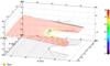 |
Fig. 43 β = 1.5, Q/m = 1.5 C/kg. Start year 2000, at −50 AU from the Sun. The particles are focused towards the solar equatorial plane, but a void region downstream of the Sun is visible that resembles the a β-cone. Figure 45 completes this picture. |
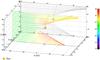 |
Fig. 44 β = 1.5, Q/m = 1.5 C/kg. Start year 1990, at −50 AU from the Sun. The particles are defocused from the solar equatorial plane. |
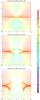 |
Fig. 45 Cross-section of the trajectories during the focusing phase of the solar cycle. Start year was 2000, β = 1.5, Q/m = 1.5 C/kg. A β-cone-like structure is visible, but its cross-section is not circular anymore (compare to Fig. 7). |
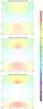 |
Fig. 46 Cross-section of the trajectories during the defocusing phase of the solar cycle. Start year was 1990, β = 1.5, Q/m = 1.5 C/kg. The void region downstream from the Sun is enhanced by the Lorentz force in comparison with the β-only case, and high dust concentrations are visible at higher latitudes. |
4.3. Application: Interstellar dust density at Saturn
We illustrate the use of the model for predictions of the ISD density at Saturn. These predictions can be used to optimize Cassini observation time or to find interstellar particles in the existing dataset. In the predictions, no gravitational focusing by planets have been accounted for; however, the enhancement in dust due to (planetary) gravitational focusing can be estimated analytically.
Figure 49 shows the position of Cassini with respect to the ISD upstream direction and the β-cones. Between mid-2001 and 2004, Saturn was in the β = 1.1 cone, and a depletion of particles with β ≥ 1.1 can be expected there. In 2006, it passes the cone for β = 1.7. In 2010, Saturn and Cassini move towards the upstream direction of the ISD. Because of the enhanced relative speed (about 36 km s-1), fluxes will be higher. Apart from the speed, also the relative density of the dust is high in 2010, since the solar minimum of the focusing cycle was in mid-2007. The year 2010 was thus a very favorable year for ISD observations for two reasons, and Cassini got prime observation time starting in 2010, where the Cassini cosmic dust analyzer (CDA; Srama et al. 2004a) was pointed towards the interstellar upstream direction.
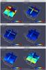 |
Fig. 47 Variation in relative densities in the solar system, due to the Lorentz force (β = 1.5, Q/m = 1.5 C/kg). Observing times are from left to right and top to bottom: 1996, 1998, 2000, 2002, 2004, 2006. The solar minimum of the defocusing cycle is in mid-1996. The maximum effect of this on the density is about 3 years later. Solar maximum is in 2002, and the solar minimum of the focusing cycle is in mid-2007. |
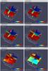 |
Fig. 48 Variation in relative densities in the solar system, due to the Lorentz force (β = 1.5, Q/m = 1.5 C/kg). Observing times are from left to right and top to bottom: 2008, 2010, 2012, 2014, 2016, 2018. The solar minimum of the focusing cycle is in mid-2007. The maximum effect of this on the density is about 3 years later. Solar maximum is in 2013, and the solar minimum of the next defocusing cycle is in mid-2018. |
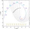 |
Fig. 49 Position of Cassini with respect to the interstellar dust flow and the β-cones. |
In Fig. 50 we show the predicted relative flux of ISD with respect to infinity at Saturn and for three particle sizes close to the adapted astronomical silicate β-curve (see Table 4: 0.3 μm, 0.2 μm and 0.06 μm). For the 0.3 μm-particles, no β-cone is present downstream from the Sun since β = 1, but a decrease in flux is visible in 2000 due to the interaction with the IMF. The solar minimum of the defocusing cycle is in mid-1996. In contrast, the focusing cycle causes an enhancement in ISD particles around 2010. For 0.2 μm particles, there is a strong depletion between 1998 and 2005. This is due to a combination of the Lorentz forces and the passage of Saturn through the β-cone of β = 1.5. There are no ISD particles of this size expected at Saturn during this time (assuming they are astronomical silicates). The effect of the Lorentz force (focusing cycle) is stronger for these particles than for the larger ones, which is visible in 2010. Finally, for very small particles of 0.06 μm (hypothetically assuming that they were able to enter the heliosphere), there is a depletion between 1995 and 2005. This is purely an effect of the Lorentz force, since β = 1 also here. The graph indicates that there are times when the small particles may reach the inner solar system and times when they do not. However, for such small particles, other forces like solar wind drag start to play a role and may diminish the effect of the concentrations of small dust(Gustafson 1994; Mukai & Yamamoto 1982).
To illustrate the effects of the (effective) solar radiation pressure force and the Lorentz force, we varied the β-value for the 0.3 μm particles between β = 0.7 and β = 1.5 while keeping the charge-to-mass ratio constant (see Fig. 51). For β < 1, there is an increase in relative flux in 2002 when Saturn is “downstream” of the Sun. For β = 1 and Q/m = 0.5, there is a reduction in the relative flux because of the Lorentz force, and for β > 1, the influence of the β-cone is clearly visible when comparing the curve with the one of β = 1.
 |
Fig. 50 Relative flux with respect to Saturn (smoothed with a width of 200 days), and scaled to the incoming flux. Three particle populations are shown close to the adapted astrosilicates β-curve (0.3 μm, 0.2 μm, and 0.06 μm). |
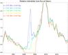 |
Fig. 51 Relative flux with respect to Saturn (smoothed with a width of 200 days), and scaled to the incoming flux. Five different β-values are shown, and Q/m is fixed at 0.5 C/kg. This is to illustrate the effect of β. |
Apart from densities or fluxes, we also predict and show the evolution of the ISD directionality (in the ecliptic frame) with time, for the same particle sizes (see Fig. 52). The direction of 0.3 μm particles is determined by the Lorentz force, since β = 1. There is a variation of about 15° in latitude and 4° in longitude over 30 years of time. The directionality of the 0.2 μm particles shows a clear influence of the β-cone: just before Saturn enters the β-cone in 1998, the (downstream) latitude increases because Saturn (at the entrance of the cone) is in the northern part of the β-cone, where particles are deflected slightly northwards. The (downstream) longitude will decrease, because ISD particles are deflected towards the vernal equinox at the entrance side (the vernal equinox side) of the cone. In contrast, when Saturn leaves the β-cone, the longitude will be higher, and will decrease again to the value of infinity (79° downstream), while the latitude will also be higher (as at entrance of the cone), and then decrease to the latitude at infinity (−8°), in the ideal case without Lorentz force. However, the change in longitude and latitude is for 0.2 μm-particles already strongly influenced by the Lorentz force, with a total spread of about 50° in longitude and 40° in latitude. For very small particles (0.06 μm), the latitudes and longitudes are governed by Lorentz forces (β = 1) and show a spread of 40° in longitude and 80° degrees in latitude.
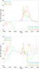 |
Fig. 52 Absolute directionality of the ISD in the ecliptic frame (upper plot: longitude, lower plot: latitude), with time, at Saturn location, for the three different ISD populations close to the adapted astrosilicates β-curve (0.3 μm, 0.2 μm, and 0.06 μm). |
Finally, this information can be used to find ISD particles in the dataset of missions like Cassini. Figure 53 shows the (integrated) sensitivity of the Cassini CDA instrument projected on the sky (ecliptic coordinates) and integrated over time (2004 until 2010). It mainly shows how long the instrument has been pointed in any given direction of the sky, between 2004 and 2010. The expected (upstream) directions are plotted as crosses for dust grains with β = 1.1, Q/m = 0.59 C/kg (upper plot) and β = 1.5, Q/m = 1.5 C/kg (lower plot). The colors show the year of impact, and the apparent motion of the spacecraft with respect to the dust is taken into account, resulting in a wider apparent spread on the instrument field of view. The plot indicates both the spread of particles across the sky and which portion of these we have theoretically been able to observe with Cassini, for a certain particle population and the time considered in the integration.
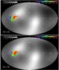 |
Fig. 53 Integrated sensitivity map of the Cassini Cosmic Dust Analyser, over the years 2004 until 2010. The crosses are simulations of dust impacts, colored according to impact year. The plot is drawn in the ecliptic frame and abberation due to spacecraft motion is taken into account. This “smears” out the directionality of the dust impacts over the instrument field of view. The upper plot shows the simulated impacts for dust with β = 1.1, Q/m = 0.59 C/kg, and the lower plot shows the simulated impacts for β = 1.5, Q/m = 1.5 C/kg. The whiter the background color, the longer Cassini CDA has been pointed towards that region of the sky. |
5. Summary
The solar system is plowing through a cloud of interstellar material consisting of gas and dust, at a speed of 26 km s-1. Viewed from inside the heliosphere, the flow of interstellar matter arrives from about 259° ecliptic longitude and 8° latitude. Previous theoretical studies have shown that interstellar grains of smaller radii than 0.1 μm are carried by the bow shock winds around the heliosphere and will not enter it (Linde & Gombosi 2000). Bigger interstellar grains enter the heliosphere and are scattered by heliospheric effects during their several decades’ long travel through the heliosphere. Scattering by solar gravitation of the flow of particles bigger than about one micron radius (thus β < 1) leads to enhanced dust densities downstream of the Sun. However, smaller interstellar grains travelling through the solar system are strongly affected by other forces than solar gravitation alone. Solar radiation pressure reduces gravity and even prevails over gravity for particle sizes between about 0.1 and 0.3 μm (assuming astronomical silicates). When β, the ratio of radiation pressure force over solar gravitational force, exceeds the value 1, particles are repelled from the Sun and cannot enter a paraboloidal exclusion zone around the Sun; e.g., particles of β = 1.3 will not get closer to the Sun than 1 AU. Since both radiation pressure and gravitational force depend on heliocentric distance r2, β is approximately constant in the solar system. Taking only solar gravity and radiation pressure into account, the trajectories of interstellar grains are attractive or repulsive hyperbolas depending on β < 1 or β > 1, respectively. For β = 1 their trajectories are straight lines because gravity and radiation pressure cancel each other out.
The Ulysses spacecraft monitored the interstellar flow of submicron-sized particles for 15 years starting in 1992. It was found that the dominating flux consists of approximately 0.3 μm particles that had a maximum β-value of >1 because an exclusion zone of small particles reached out to about 3 AU (Landgraf et al. 1999a). Measurements by this spacecraft found a long-term variation in the ISD flow by about a factor 3. The cause of this variation was found to be an interaction with the heliosphere.
Particles in the heliosphere are electrically charged owing to the competing effects of photoemission of electrons and charge collection from the ambient solar wind plasma. In our analysis we have assumed that the particles are charged to +5 Volts positive due to the prevailing photoeffect. Because of this, submicron ISD grains are affected by electromagnetic forces exerted by the IMF, frozen in the solar wind plasma. The IMF is characterized by the Parker model. The controlling parameter is the charge-to-mass ratio Q/m of the particles which depends on the particles radius as a-2. Preliminary investigations show that outside about 1–2 AU, small-scale and short-term variations in the magnetic field are smoothed out by the weakly interacting dust particles. Only the mean magnetic dipole field averaged over one solar rotation (25.38 days) is important and has been considered in this study. Within 1 to 2 AU, a full simulation of the revolving solar magnetic field has to be performed in order to accurately model the trajectories of interstellar grains. This will be done in a subsequent study. On the other hand, long-term variations due to the solar cycle (22 years) during which the dipole reverses its polarity twice have a significant effect on the dust flow. The magnetic field is carried by the solar wind at a speed of about 400 km s-1 and is stretched out to form a “Parker spiral”. Outside 1 AU from the Sun, the azimuthal component of the magnetic field dominates near the ecliptic plane leading to a north/south deflection of the particles, depending on the magnetic polarity and the position of the particles.
Since the azimuthal field strength varies only with  , the Lorentz
force decreases with r-1, i.e. the Lorentz force becomes
relatively stronger with distance from the Sun with respect to solar gravity and radiation
pressure forces. At the outer edge of the heliosphere (≈ 100 AU), the Lorentz force is
comparable to solar gravity for micron-sized particles, whereas at Saturn’s distance this is
only true for 0.5 μm particles. At the Earth’s distance scattering by
electromagnetic forces exceeds gravitational and radiation pressure forces for particles
<0.2 μm radius.
, the Lorentz
force decreases with r-1, i.e. the Lorentz force becomes
relatively stronger with distance from the Sun with respect to solar gravity and radiation
pressure forces. At the outer edge of the heliosphere (≈ 100 AU), the Lorentz force is
comparable to solar gravity for micron-sized particles, whereas at Saturn’s distance this is
only true for 0.5 μm particles. At the Earth’s distance scattering by
electromagnetic forces exceeds gravitational and radiation pressure forces for particles
<0.2 μm radius.
We found that the range of particles observed by Ulysses reached from “hardly affected” by radiation pressure and electromagnetic effects (>~1 μm) to “dominated” by electromagnetic force (~0.1 μm). However, we found that these tiny particles are strongly depleted from their abundance at the heliospheric boundary because of strong electromagnetic scattering that reduces their density in the inner planetary system. The spread in velocities due to electromagnetic accelerations and decelerations varies typically from a few km s-1 up to 50 km s-1 for the smallest particles. For trajectories of bigger particles than 0.5 μm with Q/m < 1.5, we can use straight line approximation upstream down to Saturn’s orbit, while a full simulations is needed close to the Sun and downstream from the Sun.
During about 11 years when the solar magnetic north pole is in the southern hemisphere, interstellar grains are deflected towards the solar rotational equator (i.e. close to the ecliptic plane). This is the focusing period when the flux of interstellar grains is at maximum near the ecliptic, except in the regions prohibited by radiation pressure. The flow of interstellar grains is no longer axial symmetric as in the case of gravity and radiation pressure alone.
Eleven years before and after, it is reduced by a factor ~3 as observed by Ulysses mostly due to electromagnetic scattering of small particles. This is the defocusing phase, when particles are depleted close to the ecliptic plane but concentrated at higher and lower latitudes at about 10 to 20 AU above the poles of the Sun. In general, small particles stream predominantly out of the solar system at higher latitudes.
This analysis of the flow through the heliosphere of interstellar grains of various sizes and material properties as defined by their β and Q/m values provides a means to characterize these properties for measurements taken by a spacecraft in the inner heliosphere. Both the magnitude of the flux as its direction determines the particle properties β and Q/m. This method has been used in the past by (Landgraf et al. 2003) by using the effect of β and Q/m on the mass distribution. Use of ISD speed and direction in addition to mass distribution can further constrain these parameters, when more measurements are available. Future measurements of the ISD flow through the planetary system by new and more capable in-situ dust telescopes (Srama et al. 2004b; Sternovsky et al. 2010) in combination with dynamical studies like this one will revolutionize ISD research.
We assume that the particle charge does not change significantly because of the different solar wind plasma conditions.
Axis in the solar equatorial plane that points to vernal equinox at time t0.
Figures 17 and 18 look very alike, but are actually very different. In Fig. 17, the grains are focused upstream towards the Sun, pass the solar equatorial plane (“southward” from the Sun), and are then bent again towards the north, from the focusing effect of the solar cycle. In Fig. 18, the particles remain in the northern solar hemisphere because they are repelled by the Lorentz forces (defocusing phase), and are further repelled after having passed the Sun.
Acknowledgments
This work is funded by ESA through a contract with the TU Braunschweig. The authors also thank ESA for the ESAC Science Faculty funding during a visit to the ESA premises in Spain. The work was performed while being a guest at the Dust Research Group at the Max Planck Institute for Nuclear Physics in Heidelberg. Wilcox Solar Observatory data used in this study was obtained via the web site (courtesy of J.T. Hoeksema): http://wso.stanford.edu at 2011:02:17_11:18:35 PST. The authors wish to thank the referee for his/her helpful comments. This paper is dedicated to the memory of Ir. Jeroen Verhoeve and Ing. Pieter Cogghe. Jeroen was an aerospace engineer, working in the field of navigation. Pieter, an electronics engineer, was doing research on embedded image processing techniques on FPGA. They both had a good sense of humor, deep integrity and a drive to realize their dreams and ambitions.
References
- Altobelli, N. 2004, Ph.D. Thesis, Ruprecht-Karls-Universität Heidelberg [Google Scholar]
- Altobelli, N., Kempf, S., Landgraf, M., et al. 2003, J. Geophys. Res. (Space Phys.), 108, 8032 [Google Scholar]
- Altobelli, N., Kempf, S., Krüger, H., et al. 2005, J. Geophys. Res. (Space Phys.), 110, 7102 [NASA ADS] [CrossRef] [Google Scholar]
- Altobelli, N., Grün, E., & Landgraf, M. 2006, A&A, 448, 243 [NASA ADS] [CrossRef] [EDP Sciences] [Google Scholar]
- Auer, S., Kempf, S., & Gruen, E. 2007, Dust in Planetary Systems, 643, 177 [NASA ADS] [Google Scholar]
- Baguhl, M., Grün, E., & Landgraf, M. 1996, Space Sci. Rev., 78, 165 [NASA ADS] [CrossRef] [Google Scholar]
- Burns, J. A., Lamy, P. L., & Soter, S. 1979, Icarus, 40, 1 [NASA ADS] [CrossRef] [Google Scholar]
- Draine, B. T. 2009, in Cosmic Dust – Near and Far, ed. T. Henning, E. Grün, & J. Steinacker, ASP Conf. Ser., 414, 453 [Google Scholar]
- Feuerbacher, B., & Fitton, B. 1972, J. Appl. Phys., 43, 1563 [NASA ADS] [CrossRef] [Google Scholar]
- Frisch, P. C., Dorschner, J. M., Geiss, J., et al. 1999, ApJ, 525, 492 [NASA ADS] [CrossRef] [Google Scholar]
- Frisch, P. C., Bzowski, M., Grün, E., et al. 2009, Space Sci. Rev., 146, 235 [NASA ADS] [CrossRef] [Google Scholar]
- Grün, E., Zook, H., Baguhl, M., et al. 1993, Nature, 362, 428 [NASA ADS] [CrossRef] [Google Scholar]
- Grün, E., Gustafson, B., Mann, I., et al. 1994, A&A, 286, 915 [NASA ADS] [Google Scholar]
- Gustafson, B. S. 1994, Ann. Rev. Earth Planet. Sci., 22, 553 [Google Scholar]
- Gustafson, B. S., & Misconi, N. 1979, Nature, 282, 276 [NASA ADS] [CrossRef] [Google Scholar]
- Gustafson, B. S., Greenberg, J., Kolokolova, L., Xu, Y., & Stognienko, R. 2001, Interplanetary Dust (Berlin Heidelberg New York: Springer-Verlag), 509 [Google Scholar]
- Hill, J. R., & Mendis, D. A. 1981, Can. J. Phys., 59, 897 [NASA ADS] [CrossRef] [Google Scholar]
- Hoeksema, J. 2011, Wilcox Solar Observatory, http://wso.stanford.edu [Google Scholar]
- Horányi, M. 1996, Annu. Rev. Astrophys., 34, 383 [Google Scholar]
- Jones, J., & Poole, L. M. G. 2007, MNRAS, 375, 925 [NASA ADS] [CrossRef] [Google Scholar]
- Kempf, S., Srama, R., Altobelli, N., et al. 2004, Icarus, 171, 317 [NASA ADS] [CrossRef] [Google Scholar]
- Kimura, H., & Mann, I. 1999, in Meteroids 1998, ed. W. J. Baggaley, & V. Porubcan, 283 [Google Scholar]
- Krüger, F., Werther, W., Kissel, J., & Schmid, E. 2004, Rapid Commun. Mass Spectrom., 18, 103 [CrossRef] [Google Scholar]
- Krüger, H., Landgraf, M., Altobelli, N., & Grün, E. 2007, Space Sci. Rev., 130, 401 [NASA ADS] [CrossRef] [Google Scholar]
- Landgraf, M. 1998, Ph.D. Thesis, Ruprecht-Karls-Universität Heidelberg [Google Scholar]
- Landgraf, M. 2000, J. Geophys. Res., 105, 10303 [NASA ADS] [CrossRef] [Google Scholar]
- Landgraf, M., Augustsson, K., Grün, E., & Gustafson, B. A. S. 1999a, Science, 286, 2319 [NASA ADS] [CrossRef] [Google Scholar]
- Landgraf, M., Müller, M., & Grün, E. 1999b, Planet. Space Sci., 47, 1029 [NASA ADS] [CrossRef] [Google Scholar]
- Landgraf, M., Baggaley, W. J., Grün, E., Krüger, H., & Linkert, G. 2000, J. Geophys. Res., 105, 10343 [NASA ADS] [CrossRef] [Google Scholar]
- Landgraf, M., Krüger, H., Altobelli, N., & Grün, E. 2003, J. Geophys. Res., 108, 5 [CrossRef] [Google Scholar]
- Levy, E. H., & Jokipii, J. R. 1976, Nature, 264, 423 [NASA ADS] [CrossRef] [Google Scholar]
- Linde, T. J., & Gombosi, T. I. 2000, J. Geophys. Res., 105, 10411 [NASA ADS] [CrossRef] [Google Scholar]
- Mann, I. 2010, ARA&A, 48, 173 [Google Scholar]
- Morfill, G. E., & Grün, E. 1979, Planet. Space Sci., 27, 1283 [NASA ADS] [CrossRef] [Google Scholar]
- Mukai, T. 1981, A&A, 99, 1 [NASA ADS] [Google Scholar]
- Mukai, T., & Yamamoto, T. 1982, A&A, 107, 97 [NASA ADS] [Google Scholar]
- Parker, E. N. 1958, ApJ, 128, 664 [Google Scholar]
- Schwehm, G. 1976, in Interplanetary Dust and Zodiacal Light, ed. H. Elsaesser, & H. Fechtig, Lecture Notes in Physics (Berlin: Springer Verlag), 48, 459 [Google Scholar]
- Srama, R., Ahrens, T. J., Altobelli, N., et al. 2004a, Space Sci. Rev., 114, 465 [NASA ADS] [CrossRef] [Google Scholar]
- Srama, R., Srowig, A., Rachev, M., et al. 2004b, Earth Moon and Planets, 95, 211 [NASA ADS] [CrossRef] [Google Scholar]
- Staubach, P., Grün, E., & Jehn, R. 1997, Adv. Space Res., 19, 301 [NASA ADS] [CrossRef] [Google Scholar]
- Sternovsky, Z., Grün, E., Drake, K., et al. 2010, in IEEEAC No. 1291 [Google Scholar]
- Witte, M., Rosenbauer, H., Banaszkiewicz, M., & Fahr, H. 1993, Adv. Space Res., 13, 121 [NASA ADS] [CrossRef] [Google Scholar]
All Tables
β and Q/m values for nominal interstellar particles close to the hypothetical β-curve for astronomical silicates with βmax = 1.6.
All Figures
|
Fig. 1 Trajectories of interstellar dust coming into the solar system, having the same impact parameter b, but different β-values. The dotted lines show the (analytically calculated) β-cones. The dust is assumed to initially move parallel to the X-axis, for simplification. |
| In the text | |
|
Fig. 2 Numerically calculated trajectories of particles with β = 0.5, but with different impact parameters b, in the ISD frame. The dust is concentrated downstream from the Sun. The particles accelerate near the Sun, and decelerate afterwards again to their original speed. The colorbar shows the scale of the absolute particle speed with a maximum of 50 km s-1. The particles are started at −50 AU from the Sun in 1997, and reach the region of the Sun about 9.5 years later. |
| In the text | |
|
Fig. 3 Numerically calculated trajectories of particles with β = 1.6, but with different impact parameters b, in the ISD frame. The β-cone where particles with β > 1.6 cannot enter, is visible. Particles with β > 1 and no charge will decelerate near the Sun, and then accelerate again to their original speed. The colorbar shows the scale of the absolute particle speed with a maximum of 50 km s-1. The particles are started at −50 AU from the Sun in 1997, and reach the region of the Sun about 9.5 years later. |
| In the text | |
|
Fig. 4 Absolute differences in position, velocity, and direction, in “sliced” planes at different positions from the Sun along the X-axis of the ISD-frame. The difference between the case for β = 1, Q/m = 0, and β = 0.5, Q/m = 0 is shown. The red regions denote trajectory differences of more than 1 AU (left), velocity differences of more than 5 km s-1 (middle), and angular differences of more than 5 degrees (right). The plot illustrates in what extent the straight-line approximation can be used. |
| In the text | |
|
Fig. 5 Absolute differences in position, velocity, and direction, in “sliced” planes at different positions from the Sun along the X-axis of the ISD-frame. The difference between the case for β = 1, Q/m = 0, and β = 1.6, Q/m = 0 is shown. The red regions denote trajectory differences of more than 1 AU (left), velocity differences of more than 5 km s-1 (middle), and angular differences of more than 5 degrees (right). |
| In the text | |
|
Fig. 6 Cross-section of the trajectories for β = 0.5, through different YZ-planes in the ISD frame. The color denotes the particle speed in km s-1. The particles are started at 50 AU distance from the Sun. The speed of the particles is higher near the Sun. Farther away from the Sun, they slow down to their original starting speed. The density is enhanced downstream from the Sun. |
| In the text | |
|
Fig. 7 Cross-section of the trajectories for β = 1.6, through different YZ-planes in the ISD frame. The color denotes the particle speed in km s-1. The particles are started at 50 AU distance from the Sun. The particles slow down near the Sun and accelerate again towards their original speed farther away from the Sun. The β-cone is visible. |
| In the text | |
|
Fig. 8 Relative density map of ISD in the solar system up to 10 AU from the Sun, for particles with β = 1.6. The density is shown with respect to the undisturbed ISD density at infinity, and the color scale is limited to an upper relative density of 2. The β-cone for β = 1.6 is visible as a conically-shaped volume of depletion. |
| In the text | |
|
Fig. 9 Relative density map of ISD in the solar system up to 10 AU from the Sun, for particles with β = 0.5. The density is shown with respect to the undisturbed ISD density at infinity, and the color scale is limited to an upper relative density of 2. The relative density downstream of the Sun is enhanced thanks to the gravitational focusing. |
| In the text | |
|
Fig. 10 Distance to the Sun during the closest approach for ISD particles with β = 0.5 and Q/m = 0, i.e. their closest distance to the Sun projected on a plane. The axes show the original position of the ISD particles in AU, in the ISD frame, while the numbers in the contour lines show their closest approach distances. The dotted lines are the reference case where β = 1 and Q/m = 0 (particles fly in straight lines, thus the dotted contour lines are circles). The contour lines for β = 0.5 are outside of the dotted contour lines, because the ISD is focused towards the Sun (so that a larger starting area is needed to investigate the ISD in an area of e.g. 10 AU around the Sun). |
| In the text | |
|
Fig. 11 Distance to the Sun during the closest approach for ISD particles with β = 1.6 and Q/m = 0, i.e. their closest distance to the Sun projected on a plane. The axes show the original position of the ISD particles in AU, in the ISD frame, while the numbers in the contour lines show their closest approach distances. The dotted lines are the reference case where β = 1 and Q/m = 0 (particles fly in straight lines, so the dotted contour lines are circles). The particles are “pushed away” by solar radiation pressure force, so less space is needed on the starting grid to investigate a certain area in the solar system. |
| In the text | |
|
Fig. 12 Ratio of Lorentz force to “effective gravitation” for several particle sizes and at different distances from the Sun, from Landgraf (1998). |
| In the text | |
|
Fig. 13 Computed tilt of the heliospheric current sheet, from Solar Wilcox Observatory (Hoeksema 2011). |
| In the text | |
|
Fig. 14 β-curves from Kimura & Mann (1999) showing the influence of porosity on the β-value of the dust, namely a flattening of the curve. |
| In the text | |
|
Fig. 15 Overview of the simulations performed with various β and Q/m values. All simulations are done between 2010 and 2030, where densities and fluxes are binned per 100 days, and in a region of the solar system in a box of 22 AU around the Sun. The crosses denote these simulations (β and Q/m range), while the curves are three examples of β-curves: two from Kimura & Mann (1999) and one “adapted” astronomical silicates curve (Gustafson 1994). The β-curves relate the β-parameter of a material to its size. The sizes are consequently converted in corresponding charge-to-mass ratio, assuming a surface potential of +5 V and the material density according to the corresponding material (see Eq. (20)). The diamonds on the adapted astronomical silicates curve are 4 out of the 5 parameter combinations given in Table 3, that illustrate “realistic” sets of parameters for one material and their relation to particle size. |
| In the text | |
|
Fig. 16 The ISD frame and the ECL frame. |
| In the text | |
|
Fig. 17 3D-representation of a “sheet” of particle trajectories with β = 1.0 and Q/m = 0.5 C/kg, during the focusing phase of the solar cycle. The start year is 2000. The “sheet” of particles is started along the Y-axis of the ISD frame. The focusing towards the solar ecliptic plane is visible, but at the same time there is a “defocusing” in the XY-plane (see projection), downstream of the Sun. The color denotes the particle speed in km s-1. |
| In the text | |
|
Fig. 18 3D-representation of a “sheet” of particle trajectories with β = 1.0 and Q/m = 0.5 C/kg, during the defocusing phase of the solar cycle. The start year is 1990. The “sheet” of particles is started along the Y-axis of the ISD frame. While the particles are defocused with respect to the solar equatorial plane, they are focused in the XY-plane (see projection) downstream of the Sun. |
| In the text | |
|
Fig. 19 3D-representation of a “sheet” of particle trajectories with β = 1.0 and Q/m = 0.5 C/kg during the defocusing phase of the solar cycle. The start year is 1990. The particles are started in a “sheet” along the Z-axis to illustrate the defocusing effect of the Lorentz force with respect to the solar equator. In general, during the defocusing phase of the solar cycle, the particles are accelerated in the neighborhood of the Sun. Since β = 1, we only see the influence of the Lorentz forces (not the radiation pressure force or gravity). |
| In the text | |
|
Fig. 20 β = 1.0, Q/m = 0.5 C/kg. Start year is 1995. The phase of the solar cycle is just after the solar maximum from the defocusing to focusing cycle, resulting in only moderate deflections. |
| In the text | |
|
Fig. 21 3D-representation of a “sheet” of particle trajectories with β = 1.0 and Q/m = 0.5 C/kg during the focusing phase of the solar cycle. The start year is 2000. The particles are started in a “sheet” along the Z-axis to illustrate the focusing effect of the Lorentz force with respect to the solar equator. In general, during the focusing phase of the solar cycle, the particles are decelerated in the neighborhood of the Sun. Since β = 1, we only see the influence of the Lorentz forces (not the radiation pressure force or gravity). |
| In the text | |
|
Fig. 22 β = 1.0, Q/m = 0.5 C/kg. Start year is 2006. The phase of the solar cycle is just after the solar maximum from the focusing to defocusing cycle, resulting in only moderate deflections. |
| In the text | |
|
Fig. 23 Absolute differences in position (red = difference d > 1 AU), velocity (d > 5 km s-1) and direction (d > 5°) in different “sliced” planes at different distances from the Sun. The case for β = 1, Q/m = 0.5 C/kg is compared to the straight-line approximation (β = 1, Q/m = 0). Start year is 1990 at −50 AU from the Sun. The phase of the solar cycle is the defocusing phase. |
| In the text | |
|
Fig. 24 Absolute differences in position (red color = difference d > 1 AU), velocity (d > 5 km s-1) and direction (d > 5°) in different “sliced” planes at different distances from the Sun. The case for β = 1, Q/m = 0.5 C/kg is compared to the straight-line approximation (β = 1, Q/m = 0). Start year is 2000 at −50 AU from the Sun. The phase of the solar cycle is the focusing phase. |
| In the text | |
|
Fig. 25 Closest distances of the particles to the Sun, projected on a plane, during their trajectory for β = 1, Q/m = 0.5 C/kg, during the focusing phase of the solar cycle. The axes show the original position of the ISD particles in AU, in the ISD frame, while the numbers in the contour lines show their closest approach distances. The dotted lines are the reference case where β = 1 and Q/m = 0. (Particles fly in straight lines, thus the dotted contour lines are circles.) |
| In the text | |
|
Fig. 26 Closest distances of the particles to the Sun, projected on a plane, during their trajectory for β = 1, Q/m = 0.5 C/kg, during the defocusing phase of the solar cycle. The axes show the original position of the ISD particles in AU, in the ISD frame, while the numbers in the contour lines show their closest approach distances. The dotted lines are the reference case where β = 1 and Q/m = 0. (Particles fly in straight lines, thus the dotted contour lines are circles.) |
| In the text | |
|
Fig. 27 Several cross-sections through the trajectories at different distances from the Sun (− 5 AU, 0 AU, and 5 AU) in the ISD-frame. The trajectories shown are for particles with β = 1.0 and Q/m = 0.5, started in 2000 at −50 AU from the Sun. The focusing effect of the Lorentz force is visible. This plot is directly comparable to the two corresponding trajectory plots (Figs. 17 and 21). |
| In the text | |
|
Fig. 28 Several cross-sections through the trajectories at different distances from the Sun (− 5 AU, 0 AU, and 5 AU) in the ISD-frame. The trajectories shown are for particles with β = 1.0 and Q/m = 0.5, started in 1990 at −50 AU from the Sun. The defocusing effect of the Lorentz force is visible and results in a void downstream from the Sun. Several AU above the solar ecliptic plane, two regions of higher ISD particle concentrations are visible. This plot is directly comparable with Figs. 18 and 19. |
| In the text | |
|
Fig. 29 Variation in relative densities in the solar system, due to the Lorentz force (β = 1, Q/m = 0.5 C/kg). Observing times are from left to right and top to bottom: 1996, 1998, 2000, 2002, 2004, 2006. The solar minimum of the defocusing cycle is in mid-1996. The maximum effect of this on the density is about 3 years later. Solar maximum is in 2002, and the solar minimum of the focusing cycle is in mid-2007. |
| In the text | |
|
Fig. 30 Variation in relative densities in the solar system, due to the Lorentz force (β = 1, Q/m = 0.5 C/kg). Observing times are from left to right and and top to bottom: 2008, 2010, 2012, 2014, 2016, 2018. The solar minimum of the focusing cycle is in mid-2007. The maximum effect of this on the density is about 3 years later. Solar maximum is in 2013, and the solar minimum of the next defocusing cycle is in mid-2018. |
| In the text | |
|
Fig. 31 β = 1.0, Q/m = 1.5 C/kg. Start year 1990, at −50 AU from the Sun. The main effect is defocusing. |
| In the text | |
|
Fig. 32 β = 1, Q/m = 1.5 C/kg. Start year 2000, at −50 AU from the Sun. The main effect is focusing, particles are even already clearly focused upstream of the Sun. |
| In the text | |
|
Fig. 33 Cross-section of the trajectories during the focusing phase of the solar cycle. Start year was 2000, β = 1, Q/m = 1.5 C/kg. |
| In the text | |
|
Fig. 34 Cross-section of the trajectories during the defocusing phase of the solar cycle. Start year was 1990, β = 1, Q/m = 1.5 C/kg. |
| In the text | |
|
Fig. 35 Variation in relative densities in the solar system, due to the Lorentz force (β = 1, Q/m = 1.5 C/kg). Observing times are from left to right and top to bottom: 1996, 1998, 2000, 2002, 2004, 2006. The solar minimum of the defocusing cycle is in mid-1996. The maximum effect of this on the density is about 3 years later. Solar maximum is in 2002, and the solar minimum of the focusing cycle is in mid-2007. |
| In the text | |
|
Fig. 36 Variation in relative densities in the solar system, due to the Lorentz force (β = 1, Q/m = 1.5 C/kg). Observing times are from left to right and top to bottom: 2008, 2010, 2012, 2014, 2016, 2018. The solar minimum of the focusing cycle is in mid-2007. The maximum effect of this on the density is about 3 years later. Solar maximum is in 2013, and the solar minimum of the next defocusing cycle is in mid-2018. |
| In the text | |
|
Fig. 37 β = 1.0, Q/m = 3 C/kg. Start year 2000, at −50 AU of the Sun. The particles are strongly focused, even upstream from the Sun. Particles with a low impact factor are reflected, while particles with an impact factor greater than about 20 AU are seen to pass downstream from the Sun. |
| In the text | |
|
Fig. 38 β = 1.0, Q/m = 12 C/kg. Start year 2000, at −50 AU of the Sun. The particles are reflected upstream of the Sun and accelerated to high speeds. Particles with a low impact factor get far into the inner solar system (hypothetically assumed they are not already filtered at the heliosphere) and are reflected upstream of the Sun. |
| In the text | |
|
Fig. 39 β = 1.0, Q/m = 12 C/kg. Start year 1990, at −50 AU from the Sun. The particles are strongly deflected away from the solar equatorial plane, and are accelerated to high speeds on their way out of the solar system. |
| In the text | |
|
Fig. 40 Variation in relative densities in the solar system, due to the Lorentz force
(β = 1, |
| In the text | |
|
Fig. 41 Variation in relative densities in the solar system, due to the Lorentz force
(β = 1, |
| In the text | |
|
Fig. 42 β = 1.5, Q/m = 1.5 C/kg. Start year 2000, at −50 AU from the Sun. The particles are focused towards the solar equatorial plane and for low-impact parameters they are reflected upstream of the Sun. The effect is a bit stronger than without radiation pressure force (compare with Fig. 32). |
| In the text | |
|
Fig. 43 β = 1.5, Q/m = 1.5 C/kg. Start year 2000, at −50 AU from the Sun. The particles are focused towards the solar equatorial plane, but a void region downstream of the Sun is visible that resembles the a β-cone. Figure 45 completes this picture. |
| In the text | |
|
Fig. 44 β = 1.5, Q/m = 1.5 C/kg. Start year 1990, at −50 AU from the Sun. The particles are defocused from the solar equatorial plane. |
| In the text | |
|
Fig. 45 Cross-section of the trajectories during the focusing phase of the solar cycle. Start year was 2000, β = 1.5, Q/m = 1.5 C/kg. A β-cone-like structure is visible, but its cross-section is not circular anymore (compare to Fig. 7). |
| In the text | |
|
Fig. 46 Cross-section of the trajectories during the defocusing phase of the solar cycle. Start year was 1990, β = 1.5, Q/m = 1.5 C/kg. The void region downstream from the Sun is enhanced by the Lorentz force in comparison with the β-only case, and high dust concentrations are visible at higher latitudes. |
| In the text | |
|
Fig. 47 Variation in relative densities in the solar system, due to the Lorentz force (β = 1.5, Q/m = 1.5 C/kg). Observing times are from left to right and top to bottom: 1996, 1998, 2000, 2002, 2004, 2006. The solar minimum of the defocusing cycle is in mid-1996. The maximum effect of this on the density is about 3 years later. Solar maximum is in 2002, and the solar minimum of the focusing cycle is in mid-2007. |
| In the text | |
|
Fig. 48 Variation in relative densities in the solar system, due to the Lorentz force (β = 1.5, Q/m = 1.5 C/kg). Observing times are from left to right and top to bottom: 2008, 2010, 2012, 2014, 2016, 2018. The solar minimum of the focusing cycle is in mid-2007. The maximum effect of this on the density is about 3 years later. Solar maximum is in 2013, and the solar minimum of the next defocusing cycle is in mid-2018. |
| In the text | |
|
Fig. 49 Position of Cassini with respect to the interstellar dust flow and the β-cones. |
| In the text | |
|
Fig. 50 Relative flux with respect to Saturn (smoothed with a width of 200 days), and scaled to the incoming flux. Three particle populations are shown close to the adapted astrosilicates β-curve (0.3 μm, 0.2 μm, and 0.06 μm). |
| In the text | |
|
Fig. 51 Relative flux with respect to Saturn (smoothed with a width of 200 days), and scaled to the incoming flux. Five different β-values are shown, and Q/m is fixed at 0.5 C/kg. This is to illustrate the effect of β. |
| In the text | |
|
Fig. 52 Absolute directionality of the ISD in the ecliptic frame (upper plot: longitude, lower plot: latitude), with time, at Saturn location, for the three different ISD populations close to the adapted astrosilicates β-curve (0.3 μm, 0.2 μm, and 0.06 μm). |
| In the text | |
|
Fig. 53 Integrated sensitivity map of the Cassini Cosmic Dust Analyser, over the years 2004 until 2010. The crosses are simulations of dust impacts, colored according to impact year. The plot is drawn in the ecliptic frame and abberation due to spacecraft motion is taken into account. This “smears” out the directionality of the dust impacts over the instrument field of view. The upper plot shows the simulated impacts for dust with β = 1.1, Q/m = 0.59 C/kg, and the lower plot shows the simulated impacts for β = 1.5, Q/m = 1.5 C/kg. The whiter the background color, the longer Cassini CDA has been pointed towards that region of the sky. |
| In the text | |
Current usage metrics show cumulative count of Article Views (full-text article views including HTML views, PDF and ePub downloads, according to the available data) and Abstracts Views on Vision4Press platform.
Data correspond to usage on the plateform after 2015. The current usage metrics is available 48-96 hours after online publication and is updated daily on week days.
Initial download of the metrics may take a while.