| Issue |
A&A
Volume 528, April 2011
|
|
|---|---|---|
| Article Number | A35 | |
| Number of page(s) | 18 | |
| Section | Extragalactic astronomy | |
| DOI | https://doi.org/10.1051/0004-6361/200913941 | |
| Published online | 23 February 2011 | |
Evolution of the dusty infrared luminosity function from z = 0 to z = 2.3 using observations from Spitzer⋆,⋆⋆
1
Laboratoire AIM, CEA/DSM-CNRS-Université Paris Diderot, IRFU/Service
d’Astrophysique, Bât. 709, CEA-Saclay,
91191
Gif-sur-Yvette Cedex,
France
e-mail: This email address is being protected from spambots. You need JavaScript enabled to view it.
2
Max Planck Institut für extraterrestrische Physik,
Postfach 1312,
85741
Garching,
Germany
3
Spitzer Science Center, California Institute of Technology,
Pasadena,
CA
91125,
USA
4
National Optical Astronomy Observatory,
Tucson,
AZ
85719,
USA
5
UPMC Univ Paris 06, UMR7095, Institut d’Astrophysique de Paris,
75014
Paris,
France
6
CNRS, UMR7095, Institut d’Astrophysique de Paris,
75014
Paris,
France
7
National Radio Astronomy Observatory,
PO Box 2,
Green Bank, WV
24944,
USA
8
Steward Observatory, University of Arizona,
933 North Cherry
Avenue, Tucson,
AZ
85721,
USA
Received: 22 December 2009
Accepted: 11 January 2011
Abstract
Aims. We derive the evolution of the infrared luminosity function (LF) over the last 4/5ths of cosmic time using deep 24 and 70 μm imaging of the GOODS North and South fields.
Methods. We use an extraction technique based on prior source positions at shorter wavelengths to build the 24 and 70 μm source catalogs. The majority (93%) of the sources have a spectroscopic (39%) or a photometric redshift (54%) and, in our redshift range of interest (i.e., 1.3 < z < 2.3) s20% of the sources have a spectroscopic redshift. To extend our study to lower 70 μm luminosities we perform a stacking analysis and we characterize the observed L24/(1 + z) vs. L70/(1 + z) correlation. Using spectral energy distribution (SED) templates which best fit this correlation, we derive the infrared luminosity of individual sources from their 24 and 70 μm luminosities. We then compute the infrared LF at zs1.55 ± 0.25 and zs2.05 ± 0.25.
Results. We observe the break in the infrared LF up to zs2.3. The redshift evolution of the infrared LF from z = 1.3 to z = 2.3 is consistent with a luminosity evolution proportional to (1 + z)1.0 ± 0.9 combined with a density evolution proportional to (1 + z)−1.1 ± 1.5. At zs2, luminous infrared galaxies (LIRGs: 1011L⊙ < LIR < 1012 L⊙) are still the main contributors to the total comoving infrared luminosity density of the Universe. At zs2, LIRGs and ultra-luminous infrared galaxies (ULIRGs: 1012L⊙ < LIR) account for s49% and s17% respectively of the total comoving infrared luminosity density of the Universe. Combined with previous results using the same strategy for galaxies at z < 1.3 and assuming a constant conversion between the infrared luminosity and star-formation rate (SFR) of a galaxy, we study the evolution of the SFR density of the Universe from z = 0 to z = 2.3. We find that the SFR density of the Universe strongly increased with redshift from z = 0 to z = 1.3, but is nearly constant at higher redshift out to z = 2.3. As part of the online material accompanying this article, we present source catalogs at 24 μm and 70 μm for both the GOODS-North and -South fields.
Key words: Galaxy: evolution / infrared: galaxies / galaxies: starburst / cosmology: observations
Appendices are only available in electronic form at http://www.aanda.org
Full Tables B1–B4 are only available in electronic form at CDS via anonymous ftp to cdsarc.u-strasbg.fr (130.79.128.5) or via http://cdsarc.u-strasbg.fr/viz-bin/qcat?J/A+A/528/A35
© ESO, 2011
1. Introduction
The important contribution of infrared luminous galaxies (Luminous InfraRed Galaxies, LIRGs: 1011 L⊙ < LIR < 1012 L⊙; Ultra-Luminous InfraRed Galaxies, ULIRGs 1012 L⊙ < LIR) in the evolution of the star-formation rate (SFR) history of the Universe is now well established up to zs1 (Chary & Elbaz 2001; Franceschini et al. 2001; Xu et al. 2001; Elbaz et al. 2002; Metcalfe et al. 2003; Lagache et al. 2004; Le Floc’h et al. 2005; Magnelli et al. 2009). Their contribution to the SFR density of the Universe increases with redshift up to zs1 where the bulk of the SFR density occurs in LIRGs. Study of this evolution was made possible through the use of large and accurate spectroscopic and/or photometric redshift catalogs as well as deep 24 and 70 μm surveys obtained by Spitzer.
At z > 1.3, the SFR history of the Universe has been derived by several studies (Pérez-González et al. 2005; Caputi et al. 2007) using deep 24 μm imaging and infrared bolometric correction estimated from local spectral energy distribution (SED) libraries (Chary & Elbaz 2001; Lagache et al. 2003; Dale & Helou 2002). All of these studies concluded that the relative contribution of ULIRGs to the SFR density of the Universe increases with redshift, and may even be the dominant component at zs2. However, these conclusions still need to be confirmed since there are large uncertainties at high-redshift in transforming observed 24 μm flux densities to far-infrared luminosities (Papovich et al. 2007; Daddi et al. 2007a). To study the high-redshift evolution of the SFR density, one has to combine deep mid- and far-infrared observations in order to infer robust bolometric corrections and to clearly constrain the location of the break of the infrared luminosity function (LF).
At zs2, the observed 70 μm emission corresponds approximately to the rest-frame 24 μm luminosity, which was proven to be a good SFR estimator in the local Universe (Calzetti et al. 2007). The reliability of this SFR estimator seems to hold at high-redshift since the SFR of zs2 galaxies estimated from their observed 70 μm flux densities and their radio emissions are in good agreement (Daddi et al. 2007b). Thus, to get robust estimates of the SFR of distant galaxies, we decided to use deep 70 μm observations obtained by Spitzer.
The main difficulty of using 70 μm observations to study star-formation at zs2 resides in the limited depth of the existing Spitzer data, even from the very deepest observations such as those in the Great Observatories Origins Deep Survey (GOODS). In this study, we overcome this limitation by using a stacking analysis. As shown in Papovich et al. (2007) this analysis allows characterization of the 24 vs. 70 μm correlation and thus constrains the bolometric corrections to be applied to the 24 μm flux densities. Using deep 24 and 70 μm images of the GOODS-North and South fields we find that the 24 vs. 70 μm correlation observed at high redshift is significantly different from predictions by standard SED libraries. This deviation can be interpreted as a possible signature of an obscured active galactic nuclei (AGN) (Daddi et al. 2007a) or simply as a SED evolution characterized by stronger polycyclic aromatic hydrocarbon (PAH) emission (Papovich et al. 2007). Both interpretations are discussed and two different bolometric corrections are inferred. Based on these bolometric corrections we derive the infrared LF in two redshift bins (i.e., 1.3 < z < 1.8 and 1.8 < z < 2.3). For the first time these infrared LFs take into account the evolution of SED observed in high-redshift galaxies. By comparison, extrapolation from the observed 24 μm emission alone results in significant overestimates in their infrared luminosity (Papovich et al. 2007; Daddi et al. 2007a) while extrapolations from the observed 850 μm emission constrains only the most luminous ULIRGs.
Throughout this paper we will use a cosmology with H0 = 70 km s-1 Mpc-1,ΩΛ = 0.7 and ΩM = 0.3.
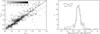 |
Fig. 1 (Left) Comparison between the photometric and spectroscopic redshifts of our 24 μm-selected catalog. This comparison is made using 1670 galaxies which have both kinds of redshifts. Dashed lines represent the relative errors found in the redshift range of our study (i.e., σΔz/(1 + z) = 0.14 for 1.3 < z < 2.3). (Right) Uncertainty in determining LIR from 24 μm fluxes densities and the Chary & Elbaz (2001) library due to error in photometric redshift estimates (black histogram). The dashed line is a Gaussian fit to this uncertainty distribution with σ = 0.15. Note that the uncertainty distribution is not Gaussian. |
Redshift catalog properties.
2. Data
2.1. Infrared imaging
The 24 μm imaging of the GOODS-N (12h36m, + 62°14′) and GOODS-S (3h32m, −27°48′) fields were obtained as part of the GOODS Legacy program (PI: Dickinson). The 70 μm data in both GOODS fields were obtained by Spitzer GO programs GO-3325 and GO-20147 (PI: Frayer). In the north they cover a region of roughly 10′ × 16′, while in the south they cover a somewhat smaller fraction of the GOODS 24 μm area, roughly 10′ × 10′. The Frayer data have been combined with additional 70 μm observations covering a wider area from the Far-Infrared Deep Extragalactic Legacy (FIDEL) program (PI: Dickinson), as well as shallower data from Spitzer guaranteed time observer (GTO) programs (PI: Rieke). While our catalog is complete to the observational limits, here we restrict our analysis to the deepest regions at 70 μm covered by the Frayer+FIDEL+GTO data, covering areas of 194 arcmin2 and 89 arcmin2 in GOODS-N and -S, respectively.
At the resolution of Spitzer at 24 and 70 μm, all sources in our fields are point sources (i.e. FWHMs5.9″ and 18″ at 24 μm and 70 μm respectively). Flux densities at these wavelengths are hence estimated using a PSF fitting technique based on the knowledge of the expected positions of the sources (Magnelli et al. 2009). For the 24 μm data, we use the position of the IRAC 3.6 μm sources as priors. This choice is motivated by the fact that the IRAC 3.6 μm data are 30 times deeper than our current 24 μm observations and that the typical S24 μm/S3.6 μm ratio spans the range [2–20] (Chary et al. 2004). Hence we can assume that all 24 μm sources have an IRAC 3.6 μm counterpart. For the 70 μm data we use as prior the IRAC positions of our flux limited sample of 24 μm sources. At this wavelength our choice is straightforward since the typical S70 μm/S24 μm ratio spans the range [2 − 100] (Papovich et al. 2007) and the 24 μm observations are about 100 times deeper than our current 70 μm observations. These assumptions are tested by visual inspection of residual images which would reveal any 24 μm or 70 μm sources missed due to the lack of priors. We find no such sources.
For GOODS-N, we use the IRAC catalog generated from the publicly available GOODS Legacy data (19437 objects detected at 3.6 μm with a 50% completeness limit of 0.5 μJy). The GOODS-S IRAC data have been incorporated into the SIMPLE IRAC Legacy Survey observations covering the wider Extended Chandra Deep Field South, also observed with MIPS as part of the FIDEL Legacy program. We use the SIMPLE IRAC catalogs (?, 61233 objects detected at 3.6 μm with a 50% completeness limit of 1.5 μJy) as priors for the MIPS source extraction over the whole FIDEL area, although here we concentrate only on the deep 10′ × 10′ GOODS-S region.
Using Monte carlo simulations we are able to estimate the quality of our 24 and 70 μm catalogs (see Magnelli et al. 2009). We find that, in both fields, the 24 and 70 μm observations reach an 80% completeness limit of 30 μJy and 2.5 mJy respectively. In the GOODS-N and S fields we detect 2151 and 870 sources respectively with S24 > 30 μJy, and 119 and 44 sources with S70 > 2.5 mJy. Tables B.1–B.4 of the online material give excerpt of the complete GOODS-N/S 24 μm and 70 μm catalogs that are now available at CDS. These catalogs extend below the 80% completeness limit, and covers the full area (approximately 10′ × 16′) of the GOODS-S region, not only the smaller 10′ × 10′ region with the deepest 70 μm imaging that is used for the analysis in this paper.
Since calibration factors taken to generate the final 24 and 70 μm mosaics are derived from stars, color corrections (at most s10%) have to be apply to all our fluxes. These color corrections being highly dependent on the redshift and the intrinsic SED of the sources, we decided to introduce these color corrections directly in the k-correction used to estimate the LF since both quantities are taken into account in this computation.
2.2. Redshifts
In this study we use spectroscopic redshifts coming from a combination of various studies (Cohen et al. 2000; Wirth et al. 2004; Cowie et al. 2004; Le Fèvre et al. 2004; Mignoli et al. 2005; Vanzella et al. 2006; Reddy et al. 2006; Barger et al. 2008; Cimatti et al. 2008; Kurk et al. in prep. for GMASS redshifts and finally Stern et al. in prep.). Photometric redshifts are computed using Z-PEG (Le Borgne & Rocca-Volmerange 2002) and all optical and near infrared data currently publicly available. In GOODS-N, optical observations in the BVIz passbands were obtained with the Advanced Camera for Surveys (ACS) onboard the Hubble Space telescope (HST) as part of the GOODS ACS Treasury program (Giavalisco and the GOODS Team, in prep.) while near infrared observations in the JK passbands were taken from the KPNO 4m FLAMINGOS catalog. In GOODS-S optical and near infrared observations were taken from the GOODS MUSIC catalog (Grazian et al. 2006; Santini et al. 2009, UBVIzJHK).
2.3. Removing AGNs
To identify and remove X-ray AGN we use deep Chandra X-Ray observations, i.e., the 1 Ms maps for GOODS-S and the 2 Ms maps for GOODS-N (Alexander et al. 2003). AGNs are identified as galaxies with either LX [0.5 − 8.0 keV] ≥ 3 × 1042 erg s-1 or a hardness ratio greater than 0.8 (ratio of the counts in the 2 − 8 keV to 0.5 − 2 keV passbands) (Bauer et al. 2004). Even if it is well-known that AGN do also harbor star formation, we do not subtract the AGN contribution to the infrared light of those galaxies since such subtraction would be highly speculative at the present level of our knowledge. Instead we conservatively decide to remove all those galaxies from our sample.
2.4. The final infrared galaxy sample
To construct our final infrared sample we first cross-match the 24 μm catalog with the X-ray observations. We find that s6%(13%) of the 24(70) μm sources contain an X-ray AGN. All those sources are excluded from our final infrared sample. Remaining sources are then matched with our spectroscopic and photometric redshift catalogs, using a matching radius of 1.5″ (i.e. sFWHM of the IRAC 3.6 μm observations). In case of multiple associations we select the closest optical counterparts. In GOODS-N (GOODS-S) 94% (92%) of the 24 μm sources brighter than 30 μJy have a spectroscopic and/or a photometric redshift and 80% (76%) of these sources have been detected in the near infrared. 46% and 37% of our 24 μm sources have a spectroscopic redshift in GOODS-S and -N respectively.
All the different steps described previously are listed in the Table 1. These steps yield to a final infrared galaxy sample containing 2644 and 138 sources detected at 24 μm and 70 μm respectively. In our redshift range of interest (i.e. 1.3 < z < 2.3) our infrared galaxy sample contains 706 sources detected at 24 μm and only 8 sources detected at 70 μm. In this redshift range, the fraction of sources with a spectroscopic redshift is s20%.
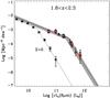 |
Fig. 2 Rest-frame 8 μm LF estimated at zs2 using the 1/Vmax method. Light blue circles and red squares represent the rest-frame 8 μm LF derived from our 24 μm sample with and without X-ray AGNs respectively. Empty triangles represent the rest-frame 8 μm LF derived by Caputi et al. (2007) at zs2. Asterisks show the local reference taken from Huang et al. (2007) and the dotted line represents the best-fit to these data points with a double power law function with fixed slopes (i.e., φ ∝ L-0.8 for L < Lknee and φ ∝ L-3.2 for L > Lknee). The dashed line represents the best fit of the rest-frame 8 μm LF at zs2 assuming that the shape of the rest-frame 8 μm LF remains the same since zs0. The dark shaded area span all the solutions obtained with the χ2 minimization method and compatible, within 1σ, with our data points. |
In Fig. 1 (left), we compare spectroscopic and photometric redshifts of 1670 sources detected at 24 μm and with both kinds of redshifts (i.e. spectroscopic and photometric redshifts). In the 1.3 < z < 2.3 redshift range, accuracy of the photometric redshifts is σΔz/(1 + z) = 0.14 and Δz/(1 + z) has a median value of − 0.002. These redshift uncertainties result in infrared luminosity uncertainties when converting 24 μm flux densities into LIR using the Chary & Elbaz (2001) library (see Fig. 1, right). Since the redshift uncertainties are not Gaussian, the infrared luminosity uncertainties are also not Gaussian: wings of the real distribution extend further away than in a Gaussian distribution. As a result, to study the real impact of redshift uncertainties on the inferred infrared LF, one needs to introduce the real redshift distribution into Monte-Carlo simulations instead of using a redshift distribution with a Gaussian statistic. Such Monte-Carlo simulations have been done and are discussed in Sect. 4.1.
To illustrate the impact on the inferred LF of the subtraction of the X-ray AGNs, we compute at zs2 the rest-frame 8 μm LF with and without X-ray AGNs. The choice of this particular redshift and wavelength is motivated by the fact that at zs2 the 24 μm observations correspond to the rest-frame 7.8 μm. Therefore the extrapolation that needs to be applied to compute the 8 μm luminosity is negligible, nearly independent of the SED library used, as well as independent of the nature of the source (i.e., AGN or star-forming galaxy). In Fig. 2 we present the rest-frame 8 μm LF derived from the 1/Vmax analysis (see Sect. 4.1 for a precise description of this method) and using the Chary & Elbaz (2001) library.
We note that the LF derived with and without the AGN are in total agreement except for the brightest luminosity bin. Even for this last luminosity bin the difference between these two LFs is relatively small and is of the order of s0.2 dex. As a result, we can conclude that our particular choice for handling AGN will not affect our final results much and will not be able to explain the large discrepancies that will arise in later sections when we compare our LFs with others that have appeared in the literature.
Our rest-frame 8 μm LF is in excellent agreement with the one inferred by Caputi et al. (2007), confirming the consistency of our 24 μm sample. We note that the LF derived in our study extends to fainter luminosities since we are using a 24 μm catalog that is ~ 3 times deeper.
3. The total infrared bolometric correction
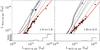 |
Fig. 3 The 70 vs. 24 μm correlations as revealed by the observations and our stacking analysis in the two redshift bins considered in this study. The empty and filled squares represent the 70 vs. 24 μm correlations observed for sources individually detected at 70 μm with photometric or spectroscopic redshift respectively. The red diamonds show the results obtained using our stacking analysis (see text). For clarity the error bars of our stacking analysis are shown only for two points. These error bars are computed using a standard bootstrap analysis and an estimate of background fluctuation using a stacking analysis at random positions (for more detail see Magnelli et al. 2009). The empty triangle shows the median correlation found in the sample of Murphy et al. (2009). The thin solid lines, the dashed lines and the triple-dots-dash lines represent the expected correlations for the CE01, the LDP and the DH libraries, respectively, at the lowest and the highest redshift of each redshift bin. The red solid line represents the inferred 24/70 μm correlation derived using a smooth linear interpolation between red diamonds and extended at high luminosities using 24 μm sources individually detected at 70 μm. At the bottom of each plot we present the fraction of 24 μm sources that are individually detected at 70 μm as a function of the 24/(1 + z) μm luminosity. |
In the local Universe tight correlations have been found between monochromatic (e.g., L15 μm, L24 μm and L70 μm ... etc.) and total infrared luminosities (LIR = L [8–1000 μm]) of galaxies (Chary & Elbaz 2001). Based on these correlations SED libraries have been developed and extensively used to estimate the total infrared luminosity of galaxies (e.g., Chary & Elbaz 2001; Lagache et al. 2003; Dale & Helou 2002, hereafter CE01, LDP, and DH1 respectively). However, it is not clear that these local templates are suitable to describe the spectral properties of distant galaxies (Papovich et al. 2007; Daddi et al. 2007b; Le Borgne et al. 2009). To study this issue, we decided to characterize the observed 24 μm vs. 70 μm correlation and compare it to the predictions of standard SED libraries. Since at high redshift (i.e. z > 1.3) most of the 24 μm sources are undetected at 70 μm, the characterization of the 24 μm vs. 70 μm correlation could only rely on mean 70 μm properties obtained through a stacking analysis. This method, which has been extensively used in the last few years, gives reliable estimates of the typical 70 μm flux density of a given galaxy population even below the detection limit of current 70 μm observations (e.g. Dole et al. 2006; Papovich et al. 2007; Magnelli et al. 2009).
We first divided our 24 μm sample into two redshift bins, of 1.3 < z < 1.8 and 1.8 < z < 2.3. Then, inside these redshift bins, we separated these 24 μm sources per luminosity bins of 0.5 dex. For each 24 μm luminosity bin we stacked on the residual 70 μm image all sources with no 70 μm detection. The photometry of the stacked image was then measured using an aperture radius of 16″, a background from within annuli of 40″ and 60″ and an aperture correction factor of 1.705 (as discussed in the Spitzer observer’s manual). Finally, the mean 70 μm flux density ( ) for a given 24 μm luminosity bin was computed following Eq. (1):
 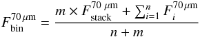 (1)where
  is the stacked 70 μm flux density of all 24 μm sources within this luminosity bin and undetected at 70 μm (sample which contains m sources);
  is the 70 μm flux density of the ith 24 μm sources within this luminosity bin and detected at 70 μm (sample which contains n sources). This procedure was performed using sliding 24 μm luminosity bins with steps of 0.1 dex. While such small sliding steps introduce correlations between our staking results, it avoids problems one might introduce by arbitrarily choosing some particular luminosity bins. Moreover, we note that since our staking analysis probes a dynamic range of s1.5 dex along the L24 μm/(1 + z) axis, there are always three independent measurements to characterize the typical L24 μm/(1 + z) − L70 μm/(1 + z) correlation.
Results of this stacking analysis are shown with filled red diamonds in Fig. 3. In both redshift bins, we find that none of the usual SED libraries can reproduce the observed correlation between L24 μm/(1 + z) and L70 μm/(1 + z). At high 24 μm/(1 + z) luminosities, standard SED libraries predict a higher L70 μm/(1 + z) to L24 μm/(1 + z) ratio than is actually observed. These low L70 μm/(1 + z) to L24 μm/(1 + z) ratio could be reproduced by standard SED libraries but would correspond to SED templates with very low intrinsic 24 μm/(1 + z) luminosities. In other words, the actual normalization of standard SED libraries which predict the increase of the L70 μm/(1 + z) to L24 μm/(1 + z) ratio with increasing 24 μm/(1 + z) luminosity is wrong. Instead, we observed that at high redshift the L70 μm/(1 + z) to L24 μm/(1 + z) ratio does not strongly depend on the 24 μm/(1 + z) luminosity and that sources with high 24 μm/(1 + z) luminosity (or equivalently high infrared luminosity) have a L70 μm/(1 + z) to L24 μm/(1 + z) ratio typical of sources in the local universe with low 24 μm/(1 + z) luminosity.
We note that among the few 24 μm sources detected at 70 μm (open and filled squares in Fig. 3) those with high 24 μm/(1 + z) luminosities (i.e. L24 μm/(1 + z) > 8 × 10¹¹ L⊙) confirm the discrepancy inferred using the stacking analysis. On the contrary, those sources with low 24 μm/(1 + z) luminosities are significantly closer to the predictions of standard SED libraries. This behavior is of course driven by selection effects and those sources only represent the high-end tail of the dispersion of the L24 μm/(1 + z) vs. L70 μm/(1 + z) correlation inferred through stacking.
We note that the discrepancies that we find between the observed L24 μm/(1 + z) vs. L70 μm/(1 + z) correlation and predictions from standard SED libraries is quite different than what we found previously for galaxies at z < 1.3 using a similar stacking analysis (Magnelli et al. 2009). There, the CE01 models provided a reasonably good fit to the observed L24 μm/(1 + z) vs. L70 μm/(1 + z) correlation.
Our findings indicate that the total infrared luminosity of a high-redshift galaxy cannot be inferred simply using its 24 μm flux density and any of the three standard SED libraries considered here. We note that this analysis is fully consistent with the results presented by Daddi et al. (2007b, see their Fig. 8) and first results obtained using Herschel data (Nordon et al. 2010). At z ~ 2 and at L24 μm/(1 + z) = 8 × 10¹⁰ and 3.5 × 10¹¹ L⊙, Daddi et al. (2007b) find that L70 μm/(1 + z) would be overestimated by a factor s2 and s10 using the CE01 library respectively, while we find a factor 2.3 and 12 respectively.
In Papovich et al. (2007) and in Murphy et al. (2009) similar discrepancies were found and explained in part as the result of an increase in the PAH emission at any given infrared luminosity in high-redshift galaxies. In both studies, the infrared luminosity of galaxies were then derived using colder SED templates (i.e., like local galaxies with lower infrared luminosities) which fit the observed correlation.
An alternative explanation for the discrepancies between SED libraries and the observed correlations can be the presence of an obscured AGN. Indeed, as suggested by Daddi et al. (2007a), the observed 24 μm flux density of a galaxy located at zs2 might be dominated by the hot dust continuum from an obscured AGN and hence it might not be a robust SFR indicator as inferred from its disagreement with radio stacking and extinction corrected UV estimates. In the same study, Daddi et al. (2007b) show that in this redshift range (1.5 < z < 2.5) the SFRs derived from radio, extinction corrected UV and 70 μm flux density agree well. This suggests that unlike 24 μm, the 70 μm passband is a good SFR indicator even in high-redshift galaxies. Thus, we will use the observed L24 μm/(1 + z) − L70 μm/(1 + z) correlation to infer L70 μm/(1 + z) for each 24 μm source and use this in turn to derive its total infrared luminosity and star-formation rate.
Based on these two explanations we decided to derive the total infrared luminosity of each galaxy using two different methods. (i) For each 24 μm source we deduce its 70 μm flux density using the L24 μm/(1 + z) − L70 μm/(1 + z) correlation. Then we choose the CE01 template whose redshifted color best matches the derived 24 to 70 μm flux ratio and renormalized it to match the 24 μm flux density of the source (i.e., ignoring the intrinsic luminosity normalization of the CE01 library; Dashed line of Fig. 4). The total infrared luminosity of this galaxy (hereafter  ) is estimated by integrating the SED curve of this template. In the following, we will assume that the uncertainties on the infrared luminosity estimated using this method is of order 0.2 dex as measured by Murphy et al. (2009). We note that the L70 μm/(1 + z)/L24 μm/(1 + z) ratio is nearly constant over the whole L24 μm/(1 + z) luminosity range and corresponds to that expected for a CE01 template with an intrinsic Log(LIR [L⊙] )s10.8. Such SED templates exhibit strong PAH features. (ii) For each 24 μm source, a 70 μm flux density is derived using the L24 μm/(1 + z) − L70 μm/(1 + z) correlation. LIR (hereafter
  ) is then simply estimated using the CE01 template (i.e., keeping the intrinsic luminosity normalization) matching the derived value of L70 μm/(1 + z).
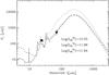 |
Fig. 4 Different infrared bolometric corrections applied to a zs1.8 galaxy. Black square represents the observed 24 μm flux density while the black star represents the 70 μm flux density predicted using the L24 μm/(1 + z) − L70 μm/(1 + z) correlation. Dotted line and the dashed-dot line represent the unscaled CE01 templates corresponding respectively to the observed 24 μm and the predicted 70 μm flux densities. The dashed line represents the scaled CE01 template which best fit the 24 and 70 μm flux densities of this galaxy. |

Figure 4 illustrates these two different bolometric corrections for a galaxy situated at z = 1.8. We note that fitting the 24 and 70 μm measurements together, allowing the renormalization of the CE01 SED templates, or using the luminosity-normalized CE01 library to fit the 70 μm alone give nearly the same results (for all our 24 μm sample we find  and
and ![Mathematical equation: \hbox{$\sigma[{\rm Log}(L_{\rm IR}^{\rm fit}/L_{\rm IR}^{70})]\thicksim0.05$}](/articles/aa/full_html/2011/04/aa13941-09/aa13941-09-eq145.png) ). Indeed, both techniques involve the use of SED templates with lower intrinsic infrared luminosity than from the 24 μm alone. We also note that using the 24 μm flux density alone and the luminosity-normalized CE01 library we would have overestimated the total infrared luminosity of this galaxy by s0.4 dex.
). Indeed, both techniques involve the use of SED templates with lower intrinsic infrared luminosity than from the 24 μm alone. We also note that using the 24 μm flux density alone and the luminosity-normalized CE01 library we would have overestimated the total infrared luminosity of this galaxy by s0.4 dex.
4. The infrared luminosity function
4.1. Methodology
The infrared LFs are derived using the standard 1/Vmax method (Schmidt 1968). The comoving volume associated with any source of a given luminosity is defined as Vmax = Vzmax − Vzmin where zmin is the lower limit of the redshift bin, and zmax is the maximum redshift at which the object could be seen given the flux density limit of the sample, with a maximum value corresponding to the upper limit of the redshift bin. For each luminosity bin, the LF is then given by  (2)where Vmax is the comoving volume over which the ith galaxy could be observed, ΔL is the size of the luminosity bin, and wi is the completeness correction factor of the ith galaxy. wi equals 1 for sources brighter than S24 μms100 μJy and decreases at fainter flux densities due to the incompleteness of the 24 μm catalog. These completeness correction factors are robustly determined using Monte-carlo simulations (Magnelli et al. 2009) and reach at most a value of 0.8. None of the conclusions presented here strongly rely on this correction.
Uncertainties in the infrared LF values depend on photometric redshift uncertainties (see Fig. 1). In particular, catastrophic redshift errors (i.e. Δz/(1 + z) > 0.15), which can shift a low redshift galaxy to higher redshift and vice versa, can modify the number density of LIRGs and ULIRGs in a given redshift bin. To estimate the effect of these catastrophic redshift errors on the derived infrared LF, one needs to have a complete census on the population of infrared galaxies at all redshifts. To simulate this, we first generate a reference catalog (i.e., an ideal sample with no redshift uncertainties), then from this reference catalog we generate 1000 mock catalogs with realistic redshift uncertainties and finally we compare the infrared LF inferred from the reference catalog with the infrared LF inferred from the 1000 mock catalogs. The key point of these simulations is to introduce redshift uncertainties which accurately reproduce the observed distribution of spectroscopic versus photometric redshifts (see Fig. 1) instead of using a standard Gaussian distribution which would not be realistic (see discussion in Sect. 2.2).
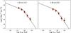 |
Fig. 5 Results of our Monte Carlo simulations. Black lines represent the infrared LF that one would have inferred using an ideal sample with no redshift or bolometric correction uncertainties. Red squares show the mean infrared LF inferred using our 1000 mock catalogs. Error bars correspond to the dispersion observed in our 1000 Monte Carlo simulations. |
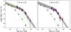 |
Fig. 6 Infrared LF estimated in two redshift bins with the 1/Vmax method. Red and dark blue squares are obtained using |
The reference catalog is constructed as follows. We first start from a simulated catalog generated from the model of Le Borgne et al. (2009) that best fits number counts of sources at 15, 24, 70, 160, 850 μm. This catalog, which contains all infrared sources that should be observed over a field of 283 arcmin2 with 0 < z < 5, reproduces the observed infrared LF up to zs1.3 (e.g., see Fig. 12 of Magnelli et al. 2009). We only keep sources with 0 < z < 1.3 or z > 2.3. Then from our observed infrared LF (Sect. 4.2) we construct and add to this catalog all infrared sources that should be observed at 1.3 < z < 2.3 over a field of 283 arcmin2. This catalog, which by construction reproduces all the observed infrared LF from z = 0 up to zs2.3, will be our reference catalog.
Starting from this reference catalog we create 1000 mock catalogs which contain the same number of sources as the original one but we attribute to each source a new redshift randomly selected to reproduce the observed distribution of spectroscopic versus photometric redshifts (see Fig. 1). To take into account the bolometric correction uncertainties not associated with the photometric redshift errors, we attribute to each source a new infrared luminosity selected inside a Gaussian distribution centered at the original source luminosity and with a dispersion of 0.2 dex (see Sect. 3). Using these 1000 mock catalogs, we then compute the infrared LF and study the difference between these infrared LFs and the infrared LF derived from the reference catalog.
Using these Monte Carlo simulations, we find only small systematic offsets between the real infrared LF and the one inferred in presence of redshift uncertainties (see Fig. 5). At zs2 and at faint luminosities, we underestimate the LF values by at most 0.1–0.15 dex while at bright luminosities we overestimate the LF values by at most 0.1–0.2 dex. These systematic offsets are smaller than the total uncertainty in each luminosity bin (s0.25 dex) defined as the quadratic sum of the Poissonian error ( ∝  ) and the dispersion given by the Monte Carlo simulations. As a result, in the following we do not correct the inferred LF for these systematic offsets.
4.2. Results
In Fig. 6, we present the infrared LF derived in two redshift bins (1.3 < z < 1.8 and 1.8 < z < 2.3) using our two different infrared bolometric corrections (red and blue squares for and respectively, see Tables A.6 and A.7). First, we note that the infrared LFs derived using these two different bolometric corrections are in very good agreement and certainly within the error bars. Here on, we will refer to the LF derived using as the infrared LF. Indeed we have a better understanding of the uncertainties of this technique and this bolometric correction was found to be reliable up to zs2 by Murphy et al. (2009).
We take as a local reference the infrared LF derived by Sanders et al. (2003), showing their data points (stars) and their best double power law fit (i.e., φ ∝ L-0.6 for Log (L/L⊙) < 10.5 and φ ∝ L-2.15 for Log (L/L⊙) > 10.5). Then, using a χ2 minimization, we fit our infrared LFs with the same function, fixing the power law slopes at their zs0 values and leaving Lknee and φknee as free parameters (see Table 2). The shaded regions present all the solutions which are compatible with the data within 1σ. These shaded regions extend to luminosities lower than our current observations and strongly depend on the assumption we made on the shape of the infrared LF, i.e. that it remains the same since zs0. We will see latter on that this assumption is quite consistent with observational constraints obtained on the low luminosity end of the infrared LF (Reddy et al. 2008).
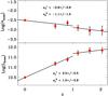 |
Fig. 7 Evolution of φknee and Lknee as function of redshift. Data points below z = 1.3 are taken from Magnelli et al. (2009). |
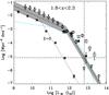 |
Fig. 8 The infrared LF at zs2 obtained in this work (dark shaded area and dashed line) as compared with the determinations of other authors. The infrared LF at zs2 obtained by Caputi et al. (2007, we are using their double exponential function) is represented by the dashed dotted line. Empty circles represent the infrared LF at zs2 inferred by Pérez-González et al. (2005). Empty diamonds represent the infrared LF at zs2.3 inferred by Reddy et al. (2008). Empty triangles represent the infrared LF at zs2.5 inferred by Chapman et al. (2005). Filled black diamonds and empty squares represent the infrared LF that we would have inferred using our 24 μm sample and the unscaled LDP or CE01 SED libraries respectively. The horizontal dashed line presents the source density below which the number of sources in the volume of GOODS and in a luminosity bin of 0.5 dex is less than 2. The vertical dashed line represents the corresponding luminosity using the best fit of our infrared LF. |
Parameter values of the infrared LF.
The evolution of Lknee and φknee between z = 1.3 and z = 2.3 is compared in Fig. 7 with the evolution found at lower redshifts by Magnelli et al. (2009). Assuming that the shape of the LF remains the same since zs0, we express the evolution of the infrared LF as ρ(L,z) = g(z)ρ(L/f(z),0), where g(z) and f(z) describe the density and the luminosity evolution through g(z) = (1 + z)p and f(z) = (1 + z)q. Between z = 0 and zs1 the redshift evolution consists mainly of a slight density evolution proportional to (1 + z)−0.9 ± 0.6 and a luminosity evolution proportional to (1 + z)3.5 ± 0.5. Then between zs1 and zs2 we observe a density evolution proportional to (1 + z)−1.1 ± 1.5 associated with a luminosity evolution proportional to (1 + z)1.0 ± 0.9. In comparison, at z > 1 Caputi et al. (2007) find a density evolution proportional to (1 + z) − 3.9 ± 1.0 and a luminosity evolution proportional to (1 + z)2.2 ± 0.5. The evolution of the infrared LF that we find at z > 1.3 is more gradual than that derived by Caputi et al. (2007) and is nearly consistent with no evolution.
Appendix A presents the evolution of the rest-frame 8, 15, 25, 35 μm LFs. Rest-frame luminosities of each source are derived using the SED that we used to compute its .
4.3. Comparison with previous work
In Fig. 8 we compare our results at zs2 with the infrared LF inferred in various previous studies. There is a clear disagreement between our results and the infrared LF derived by Caputi et al. (2007). This discrepancy arises from the fact that the bolometric corrections used in Caputi et al. (2007, i.e. with the LDP library) do not take into account the SED evolution that we observe at high redshift. Using the same bolometric corrections as Caputi et al. (2007) does lead us to similar results (see black diamonds of Fig. 8). The disagreement of our results with the LF from Pérez-González et al. (2005) is even larger because they compute their bolometric corrections using the CE01 library (see open squares in Fig. 8), i.e. the standard SED library which exhibit the largest discrepancies with the observed L24 μm/(1 + z) − L70 μm/(1 + z) correlation at z > 1.3 (see Sect. 3). Rodighiero et al. (2010) have also derived the zs2 infrared LF using deep 24 μm observations of the VVDS-SWIRE (S24 μm > 400 μJy) and GOODS (S24 μm > 80 μJy) fields. Data points from this study are not shown in Fig. 8 since they are very similar to that from Caputi et al. (2007) (see Fig. 15 of Rodighiero et al. 2010).
In Fig. 8, we also compare our results with the infrared LF inferred at zs2.3 by Reddy et al. (2008) using observations of UV-selected star-forming galaxies. This study derived SFR and dust reddening from the UV rest-frame observations calibrated by comparison to 24 μm photometry for brighter sources. The UV-derived extinction was used to compute the expected infrared emission from galaxies fainter than the 24 μm detection limit and hence provide an extension of the IR LF to fainter luminosities. We find good agreement between our LF and that of Reddy et al. in the range of luminosities where the two studies overlap. At faint luminosities (log (LIR/L⊙) < 11) our best fit LF falls somewhat below that derived by Reddy et al. (2008), although they are still consistent within the uncertainties. We have no direct measurements with Spitzer at such faint luminosities and rely upon an extrapolation based on a faint-end slope fixed at its z ~ 0 value. As detail in Sect. 4.4 this disagreement at faint luminosities has nearly no impact on the SFR density inferred at zs2. Indeed, the integrated SFR density of the universe at zs2 computed from our LF agrees with that derived by Reddy et al. (2008).
Finally we compare our results with the infrared LF inferred at zs2.5 by Chapman et al. (2005) using submillimeter observations2. The luminosity range probed by Chapman et al. (2005) is not constrained by our study since the comoving volume probed by the GOODS survey is too small (i.e., fewer than 2 sources would be present in this volume for a luminosity bin of ΔLog(LIR) = 0.5 dex). We note however that the extrapolation of our infrared LF to high luminosities is consistent with the estimates of Chapman et al. (2005).
4.4. Discussion
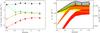 |
Fig. 9 (Left) Evolution up to zs2.3 of the comoving number density of “normal” galaxies (i.e. 107 L⊙ < Lir < 1011 L⊙; black filled triangles), LIRGs (orange filled diamonds) and ULIRGs (red filled stars). The green circles represent the total number of galaxies which are above the 24 μm detection limit of the surveys presented here, i.e. |


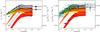 |
Fig. 10 (Left) Evolution of the comoving IR energy density up to zs2.3. Blue empty circles represent the results obtained by Caputi et al. (2007) for the global evolution of the comoving energy density (solid line) and the relative contribution of “normal” galaxies (dot line), LIRGs (dashed line) and ULIRGs (dot dashed line). Filled black star represents the comoving IR energy density of the Universe inferred at zs2.3 by Reddy et al. (2008) while open star shows the relative contribution of LIRGs. Filled areas are as in Fig. 9. (Right) Evolution of the comoving SFR density up to zs2.3 assuming that SFR and LIR are related by Eq. (3) for a Salpeter IMF. Filled areas are as in Fig. 9. The dotted line represents the SFR measured using the UV light not corrected for dust extinction (Tresse et al. 2007). The dashed line represents the total SFR density defined as the sum of the SFR density estimated using our infrared observations and the SFR density obtained from the UV light uncorrected for dust extinction. Light blue diamonds are taken from Hopkins & Beacom (2006) and represent the SFR densities estimated using various estimators. Dark blue triangles represent the SFR density estimated by Seymour et al. (2008) using deep radio observations. Green circles represent the SFR density estimated by Smolčić et al. (2009) using deep 20 cm observations and dark blue squares represent the relative contribution of ULIRGs to this SFR density. |
We derive the evolution of the comoving number density of LIRGs and ULIRGs by integrating the infrared LF at z = 1.55 ± 0.25 and z = 2.05 ± 0.25. We then combine these estimates with the evolution found at 0 < z < 1.3 by Magnelli et al. (2009) (Fig. 9left). We find that the number densities of LIRGs and ULIRGs between zs1.3 and zs2.3 are nearly constant. The number density of ULIRGs at z ~ 2 ( Mpc-3) agrees with estimates made by Daddi et al. (2007b) (s10 × 10-5 Mpc-3) using UV observations calibrated against radio and other non-24 μm data. However, if we compare our number density with the Daddi et al. (2007b) estimate obtained combining UV and 24 μm observations (
 Mpc-3) we find a clear disagreement.
Figure 9 (right) presents the evolution of the comoving infrared luminosity density (IR LD; or, equivalently, SFR density under the assumption that the SFR and LIR are related by Eq. (3) for a Salpeter IMF, i.e. φ(m) ∝ m-2.35, between 0.1–100 M⊙, Kennicutt 1998) produced by ULIRGs, LIRGs, and by galaxies with LIR < 1011 L⊙ (hereafter called “normal” galaxies by analogy with ordinary spiral galaxies at zs0, although we note that at high redshift, LIRGs and ULIRGs themselves are sufficiently common to be considered “normal” for their epoch). We find a slight decrease of the IR LD from z = 1.3 to z = 2.3 due to a decrease in the contribution of LIRGs and “normal” galaxies. At zs2 the IR LD of the Universe is still dominated by LIRGs and not by ULIRGs, contrary to previous claims (e.g., Pérez-González et al. 2005). Using the best fit of our infrared LF, we infer that at zs2 LIRGs and ULIRGs have an IR LD of 4.5 × 10⁸ L⊙ Mpc-1 and 1.5 × 10⁸ L⊙ Mpc-1 respectively and that they account for 49% and 17% of the total IR LD respectively. ![Mathematical equation: \begin{equation} \label{eq:SFR_Lir} {\it SFR}~ [{M}_{\odot}~ {\rm yr}^{-1}] = 1.72 \times 10^{-10} L_{\rm IR} ~[{L}_{\odot}]. \end{equation}](/articles/aa/full_html/2011/04/aa13941-09/aa13941-09-eq221.png) (3)We compare our estimates with the evolution derived by Caputi et al. (2007) (Fig. 10left). At zs2 we find that the IR LD of ULIRGs estimated from our best fit is a factor of s1.8 lower than that estimated by Caputi et al. (2007). For LIRGs, for which we still have a good constraint due to our deep 24 μm sample, our estimate of their IR LD is a factor of s1.5 higher than that inferred by Caputi et al. (2007). Nevertheless, we note that if we take into account the range of IR LD defined by all solutions compatible within 1σ with our data points, our IR LDs of LIRGs and ULIRGs are compatible with estimates from Caputi et al. (2007). On the other hand, the IR LD estimated by Caputi et al. (2007) for galaxies with LIR < 1011 L⊙ is far below our estimate since they used a flatter faint-end slope for their infrared LF. We believe that our estimate is more reliable since we are using a 24 μm catalog that is ~ 3 times deeper than that used by Caputi et al. (2007). We also note that the extrapolation of our infrared LF to these faint luminosities is corroborated by the infrared LF inferred by Reddy et al. (2008).
(3)We compare our estimates with the evolution derived by Caputi et al. (2007) (Fig. 10left). At zs2 we find that the IR LD of ULIRGs estimated from our best fit is a factor of s1.8 lower than that estimated by Caputi et al. (2007). For LIRGs, for which we still have a good constraint due to our deep 24 μm sample, our estimate of their IR LD is a factor of s1.5 higher than that inferred by Caputi et al. (2007). Nevertheless, we note that if we take into account the range of IR LD defined by all solutions compatible within 1σ with our data points, our IR LDs of LIRGs and ULIRGs are compatible with estimates from Caputi et al. (2007). On the other hand, the IR LD estimated by Caputi et al. (2007) for galaxies with LIR < 1011 L⊙ is far below our estimate since they used a flatter faint-end slope for their infrared LF. We believe that our estimate is more reliable since we are using a 24 μm catalog that is ~ 3 times deeper than that used by Caputi et al. (2007). We also note that the extrapolation of our infrared LF to these faint luminosities is corroborated by the infrared LF inferred by Reddy et al. (2008).
We also compare our zs2.05 IR LD values with the zs2.3 estimates of Reddy et al. (2008). We note that this comparison is not straightforward because their IR LD needs to be slightly corrected prior to be compared with our work. Indeed, since they cannot constrain with their sample the contribution of ULIRGs to the IR LD, they use the value derived by Caputi et al. (2007). By replacing the Caputi et al. (2007) estimates by our value we compute the correct IR LD of Reddy et al. (2008), i.e., 10.0 ± 0.2 × 10⁸ L⊙ Mpc-3. We find that the IR LDs derived by Reddy et al. (2008) for LIRGs and for the integrated population of all galaxies agree with our values. This agreement reinforces the idea that at zs2 UV corrected for extinction is a good SFR indicator (Daddi et al. 2007b).
In order to get a complete census on the SFR history we need to take into account the contribution of unobscured UV light. The unobscured SFR density (dotted line in Fig. 10right) is taken from Tresse et al. (2007) and corresponds to the SFR density inferred using UV observations not corrected for extinction. The total SFR density (dashed line in Fig. 10right) is then defined as the sum of the unobscured SFR density traced by the direct UV light and the dusty SFR density traced by the infrared emission. We find that the relative contribution of unobscured UV light to the cosmic SFR density evolves nearly in parallel with the total one and accounts for ~ 20% of the total SFR density. Globally, the cosmic star-formation history that we derived is consistent with the combination of indicators, either unobscured or corrected for dust extinction, as compiled by Hopkins & Beacom (2006). We also notice a very good agreement between the cosmic star-formation history derived in our work and the ones derived by Seymour et al. (2008) using deep radio observations.
Our estimates can suffer from several uncertainties. Especially the contribution of “normal” galaxies to the IR LD comes from the extrapolation to low luminosities of the infrared LF where we have no constraints. To cross check our results we compute a lower limit on the comoving IR LD by stacking 70 μm images at the positions of all IRAC sources in each redshift bin of interest (i.e.,  Jy; up arrows in Fig. 9right). This analysis is possible because the correlation between L70 μm/(1 + z) and LIR is quasi-linear at this redshift, and hence ΣS(70 μm) ∝ ΣLIR. The stacking result is fully consistent with the value based on the integration of the extrapolated best fit to our infrared LF.
As discussed in Sect. 3, the role of obscured AGN on the estimate of the infrared LF is still uncertain. Such results will be debated until the Herschel infrared space observatory provides accurate far-infrared measurements for faint, high-redshift galaxies. However, as shown by Murphy et al. (2009) using IRS spectroscopy, the mid-IR continuum from an AGN appears to scale with increasing 24 μm luminosity. As a result, the removal of any additional contribution from obscured AGN activity will only steepen the bright-end of the infrared LF. This would reinforce our main result which is the fact that at zs2 previous studies have overestimated the number density of ULIRGs.
5. Conclusion
For the first time we take advantage of deep far-infrared observations to derive the evolution of the infrared luminosity density (or equivalently SFR density under the assumption that the SFR and LIR are related by Eq. (3) for a Salpeter IMF) over the last 4/5ths of the cosmic time (see Fig. 9right). Using the deepest 24 μm (s3 times deeper than any previous studies) and 70 μm observations made by Spitzer and a careful stacking analysis we are able to calibrate a new infrared bolometric correction based on the renormalization of local SED templates reproducing the observed L24/(1 + z) vs. L70/(1 + z) correlations. This new bolometric correction is a key result of our analysis, since previous studies on the infrared LF at z ~ 2 (e.g., Pérez-González et al. 2005; Caputi et al. 2007) did not account for the evolution of the infrared SEDs that we observe in high-redshift galaxies. Our main result is that we find a flattening of the SFR density between z = 2.3 and 1.3, and that the comoving number density of LIRGs and ULIRGs remain nearly constant over this redshift range. At zs2 the SFR density is still dominated by LIRGs and not by ULIRGs contrary to previous claims. The flattening of the SFR density at z > 1 reinforces the idea that at this redshift we observe a change of the properties of star-forming galaxies as already suggested by the reversal of the star formation-density relation at zs1 (Elbaz et al. 2007).
The evolution of the SFR density of the Universe provides a strong constraint on the main mechanism which triggers the SFR in galaxies. At z < 1 the decrease of the SFR density might be driven by a gradual gas exhaustion as suggested by the continuous decrease of the SFR vs. M ⋆ relation in this redshift range (Noeske et al. 2007; Elbaz et al. 2007). Between z ~ 2 and z ~ 1, the relatively constant SFR density still needs to be understood in the framework of large-scale structure formation, merging, and/or AGN activity.
The main limitation of our study is the uncertainty on the influence of obscured AGN on the infrared bolometric correction to be applied to bright 24 μm sources. This influence will soon be assessed using new far-infrared observations from Herschel. In particular, the GOODS-Herschel Open Time Key Programme (PI: David Elbaz) will reach the faintest flux limits at 100 μm in an ultradeep field within GOODS-S, expected to provide individual measurements for most z ~ 2 galaxies detected at 24 μm by Spitzer, where here we could only derive average values based on 70 μm stacking. This should help disentangle the contributions of AGN and star formation for sources over a broad swath of the high-redshift infrared luminosity function.
Online material
Appendix A: The rest-frame 8 μm, 15 μm, 25 μm and 35 μm LFs
We aim to derive the rest-frame 8 μm, 15 μm, 25 μm and 35 μm LF from our 24 μm sample. This is done here for several reasons. While the derivation of the rest-frame 8 μm LF has already been addressed in some previous studies (Caputi et al. 2007), our 24 μm sample reaches flux limits ~ 3 times fainter, providing improved constraints on the LF break. The rest-frame 15 μm LF provides continuity with what we have computed in Magnelli et al. (2009). The rest-frame 25 μm LF was not derived in Magnelli et al. (2009) but it does have several points of interest. First, it reduces the k-correction that one has to apply when observing infrared sources at zs2 using a 70 μm passband or at zs3 using a 100 μm passband. Hence, this rest-frame LF could be compared with future 70 μm and 100 μm observations made using the Photodetector Array Camera and Spectrometer (PACS) instrument onboard the Herschel satellite. Second, the rest-frame 25 μm LF offers a means to compare directly with IRAS 25 μm observations of galaxies in the local universe. Third, and perhaps most importantly, the rest-frame 25 μm luminosity has been shown to provide a reliable and fairly direct measurement of star formation in galaxies (e.g., Calzetti et al. 2007). Hence, one may want to use these measurements in the future to directly derive the SFR distribution function without using intermediate bolometric corrections. The rest frame 35 μm LF also provides continuity with quantities derived in Magnelli et al. (2009) and corresponds at zs2 to the observed 100 μm flux density. As a result, this rest-frame LF would be a standard comparison for the zs2 LF computed using PACS 100 μm observations.
The various rest-frame luminosities are derived using the same method as that used to compute  . For each 24 μm source we deduce its 70 μm flux density using the L24 μm/(1 + z) − L70 μm/(1 + z) correlation. Then we choose in the CE01 library the scaled template which best fits these 24 and 70 μm fluxes densities. Using this scaled template we then compute the rest-frame luminosities of this galaxy in our four passbands of interest (i.e., at 8 μm, 15 μm, 25 μm and 35 μm). The corresponding rest-frame LFs are computed using the 1/Vmax method. All the LF are then fitted using a double power law function with fixed slopes estimated using a bivariate method (see Table A.1).
Figure A.1 presents the rest-frame 8 μm LF derived in our two redshift bins using the 1/Vmax method. These LF are compared with the local reference of Huang et al. (2007) and with the zs2 LF derived by Caputi et al. (2007). Our estimates agree well with those of Caputi et al. (2007), but extend to lower luminosities.
Figure A.2 presents the rest-frame 15 μm LF derived in our two redshift bins using the 1/Vmax method. Comparing to the local reference of Xu (2000) and with the zs0.55, zs0.85 and zs1.15 reference of Magnelli et al. (2009), we note the strong evolution of this LF with redshift.
Figure A.3 presents the rest-frame 25 μm LF derived in our two redshift bins using the 1/Vmax method as well as the local reference of Shupe et al. (1998).
Finally Fig. A.4 presents the rest-frame 35 μm LF derived in our two redshift bins using the 1/Vmax method as well as the local reference derived from Shupe et al. (1998), and the LFs derived in Magnelli et al. (2009) at zs0.55, zs0.85 and zs1.15.
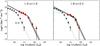 |
Fig. A.1 The rest-frame 8 μm LF estimated in two redshift bins with the 1/Vmax method. Red squares are obtained using scaled CE01 templates which best fit the L24 μm/(1 + z) − L70 μm/(1 + z) correlation. Empty triangles and blue dashed-dotted line present the rest-frame 8 μm LF obtained at zs2 by Caputi et al. (2007). Asterisks show the local reference taken from Huang et al. (2007) and the dotted line presents the best-fit to these data points with a double power law function with fixed slopes (see Table A.1). The dark shaded area span all the solutions obtained with the χ2 minimization method and compatible, within 1σ, with our data points. The dashed line represents the best fit of the rest-frame 8 μm LF. |
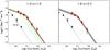 |
Fig. A.2 The rest-frame 15 μm LF estimated in two redshift bins with the 1/Vmax method. Red squares are obtained using scaled CE01 templates which best fit the L24 μm/(1 + z) − L70 μm/(1 + z) correlation. Asterisks show the local reference taken from Xu (2000) and the dotted line presents the best-fit to these data points with a double power law function with fixed slopes (see Table A.1). The dark shaded area span all the solutions obtained with the χ2 minimization method and compatible, within 1σ, with our data points. The dashed line represents the best fit of the rest-frame 15 μm LF. In the first redshift panel, we reproduce in green, blue, yellow and red the best fit of the LF obtained at 0.4 < z < 0.7, 0.7 < z < 1.0, 1.0 < z < 1.3 (Magnelli et al. 2009), and 1.8 < z < 2.3 respectively. |
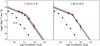 |
Fig. A.3 The rest-frame 25 μm LF estimated in two redshift bins with the 1/Vmax method. Red squares are obtained using scaled CE01 templates which best fit the L24 μm/(1 + z) − L70 μm/(1 + z) correlation. Asterisks show the local reference taken from Shupe et al. (1998) and the dotted line presents the best-fit to these data points with a double power law function with fixed slopes (see Table A.1). The dark shaded area span all the solutions obtained with the χ2 minimization method and compatible, within 1σ, with our data points. The dashed line represents the best fit of the rest-frame 25 μm LF. |
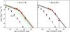 |
Fig. A.4 The rest-frame 35 μm LF estimated in two redshift bins with the 1/Vmax method. Red squares are obtained using scaled CE01 templates which best fit the L24 μm/(1 + z) − L70 μm/(1 + z) correlation. Asterisks show the local reference derived from Shupe et al. (1998) and the dotted line presents the best-fit to these data points with a double power law function with fixed slopes (see Table A.1). The dark shaded area span all the solutions obtained with the χ2 minimization method and compatible, within 1σ, with our data points. The dashed line represents the best fit of the rest-frame 35 μm LF. In the first redshift panel, we reproduce in green, blue, yellow and red the best fit of the LF obtained at 0.4 < z < 0.7, 0.7 < z < 1.0, 1.0 < z < 1.3 (Magnelli et al. 2009), and 1.8 < z < 2.3 respectively. |
Parameter values of the rest-frame 8 μm, 15 μm, 25 μm and 35 μm LF.
The rest-frame 8 μm LF derived from the 1/Vmax analysis.
The rest-frame 15 μm LF derived from the 1/Vmax analysis.
The rest-frame 25 μm LF derived from the 1/Vmax analysis.
The rest-frame 35 μm LF derived from the 1/Vmax analysis.
The infrared LF derived from the 1/Vmax analysis using .
The infrared LF derived from the 1/Vmax analysis using .
Appendix B: Source list
At the resolution of Spitzer most of the sources in our fields are point sources (i.e. FWHMs5.9″ and 18″ at 24 μm and 70 μm respectively). Therefore, to derive their photometry we decided to use a PSF fitting technique that take into account, as prior information, the expected position of the sources. Starting from IRAC positions (GOODS-N: GOODS legacy program, Dickinson et al., in prep.; GOODS-S: SIMPLE catalog, ?) we extract all 24 μm sources. Then, using our 24 μm catalogs, we extract all 70 μm sources. This method deals with a large part of the blending issues encountered in dense fields and allows straightforward multi-wavelength association between near-, mid- and far-infrared sources. The disadvantage of this method is that we have to assume that all sources present in our mid-infrared images have already been detected at IRAC wavelengths. In our case this assumption is true because our IRAC 3.6 μm data are 30 times deeper than our current 24 μm observations and that the typical S24 μm/S3.6 μm ratio spans the range [2–20].
In this online material we release our complete 24 μm and 70 μm source catalogs for both GOODS fields. These catalogs expend below the 80% completeness limit, and cover the full area (approximately 10′ × 16′) of the GOODS-S region (i.e., not only the smaller 10′ × 10′ region with the deepest 70 μm imaging that is used for the analysis in this paper). The noise level in the GOODS 24 μm data is homogeneous over most of the field, with some degradation near the edge where the exposure time is somewhat reduced. We restrict our release to regions with exposure time higher than 9500 s per pixel. This limit corresponds to a quarter of the exposure time of the deep inner region (s38 000 s). This degradation does not really affect the depth of our 24 μm catalogs in that region since uncertainties are still dominated by confusion ( Jy). At 70 μm, the noise level is roughly uniform throughout GOODS-N (s12 000 s per pixel). However, in GOODS-S the deepest 70 μm data, with noise similar to those in GOODS-N, are limited to a region approximately 10′ × 10′ in extent. The outer region portions of the GOODS-S field have somewhat shallower 70 μm data (s6000 s per pixel).
At 24 μm, sources are detected using an empirical 24 μm PSF constructed with isolated point like objects present in the mosaic. At 70 μm no reliable empirical PSF could be constructed because only a few isolated sources could be found in each map. We then decided to use the appropriate 70 μm Point Response Function (PRF) estimated on the extragalactic First Look Survey mosaic (xFLS; Frayer et al. 2006a) and available on the Spitzer web site. At both wavelengths an aperture correction is applied to all flux densities to account for the finite size of our PSFs. Those aperture corrections are taken from the Spitzer data handbook.
Calibration factors used to generate the final 24 and 70 μm mosaics are derived from stars, whose SED at these wavelengths are generally very different from those of distant galaxies. Hence, color-corrections have to be applied to all flux densities (at most s10%). In the catalogs released here, 70 μm flux densities have been color-corrected using a systematic and standard correction of 1.09 (see Spitzer data handbook). This 70 μm color-correction is computed for distant galaxies with dust temperature of s40 K. This color-correction differs from those applied in our study and which take into account the redshift of each source (see discussion in Sect. 2.1). No color–corrections are applied to our 24 μm flux densities since, for those data, color-corrections are more strongly dependent on the redshift of the source. Indeed, 24 μm data probes different part of galaxy SED as function of the redshift (black-body emission of dust or PAH emission).
Our 24 μm and 70 μm data are the deepest observations taken by Spitzer and have been designed to reach the confusion limit of this satellite. Flux uncertainties are therefore a complex combination of photon and confusion noise. In order to estimate these complex flux uncertainties and to characterize the quality of our 24 μm and 70 μm catalogs we use two different approaches. First, we compute the noise of each detection using our residual maps. Second, we estimate a statistical flux uncertainty based on extensive Monte-Carlo simulations.
Noises estimated on residual maps correspond to the pixel dispersion, around a given source, of the residual map convolved with the appropriate PSF. This method has the advantage of taking into account the rms of the map and the quality of our fitting procedure. These noise estimates are given in our released catalogs as σmap. These estimates are almost equal to the rms of our maps, i.e., σmaps3 μJy/beam at 24 μm in both GOODS-N and GOODS-S, 0.3 mJy/beam at 70 μm in GOODS-N and in the deepest region of GOODS-S, and 0.45 mJy/beam at 70 μm in the shallowest region of GOODS-S.
In order to estimate the effect of confusion noise we performed extensive Monte-Carlo simulations. We added artificial sources in the 24 μm and 70 μm images with a flux distribution matching approximately the measured number counts (see Frayer et al. 2006b; Papovich et al. 2004). To preserve the original statistics of the image (especially the crowding properties) the numbers of artificial objects added in the image was kept small (we only added 40 sources into the 24 μm images and 4 sources into 70 μm images). We then performed our source extraction method and compared the resulting photometry to the input values. To increase the statistic, we used repeatedly the same procedure with different positions in the same field. For each field we introduced a total of 20 000 artificial objects. Results of these Monte-Carlo simulations are shown in Fig. 1 of Magnelli et al. (2009) and are summarized hereafter.
MIPS sources in GOODS-N with  .
.
MIPS sources in GOODS-N with  .
.
MIPS sources in GOODS-S with .
MIPS sources in GOODS-S with  .
.
From these Monte-Carlo simulations we derive three important quantities: the photometric accuracy, the completeness and the contamination of our catalogs as function of flux density. Completeness is define as the fraction of simulated sources extracted with a flux accuracy better than 50%. The contamination is defined as the fraction of simulated sources introduced with S < 2σmap which are extracted with S > 3σmap.
Using these Monte-Carlo simulations, we find that in both GOODS fields our 24 μm catalogs are 80% complete at s30 μJy. At this flux density, the flux accuracy is better that 20% and the contamination is s10%. The flux accuracy of our source extraction reaches 33% around 20 μJy. This limit could be defined as the “real” 3σsimu limit of our data because this estimate take into account confusion noise. At 20 μJy, the completeness of our catalog is s40% and the contamination is s15%.
For our deep 70 μm data in GOODS-N and -S, Monte-Carlo simulations show that our catalogs are 80% complete at 2.5 mJy. The 33% flux accuracy is reached at 2 mJy with a completeness of s50% and a contamination of s15%. For the shallow 70 μm data of GOODS-S, the 80% completeness limit is reached at 3 mJy, and the 33% flux accuracy is reached at 2.5 mJy. At 2.5 mJy, the completeness is 45% and the contamination is 15%.
Flux uncertainties derived using our Monte-Carlo simulations are denoted by σsimu. These flux uncertainties present the advantage of accounting for nearly all sources of noise, which explains why they are almost always larger than noise estimates based on residual maps (i.e., σmap). However, this noise estimate is computed independently of the actual position of the individual sources, it is statistical. In some cases, local effects can dominate the noise as it is the case when two sources are blended. This local effect, together with the background fluctuation due to the photometric confusion noise (i.e. the noise due to sources fainter that the detection limit that were not subtracted from the image to produce the residual image), is better accounted for in the noise estimated from the residual maps, which is estimated locally. To be conservative, users should always use the highest uncertainties between σmap and σsimu, but not the quadratic combination of both since they are not independent.
Tables B.1–B.4 give excerpt of our complete GOODS-N/S 24 μm and 70 μm catalogs available at CDS. For each field we decide to split our 24 μm catalogs into two (i.e., sources with 3 < σsimu < 5 and sources with 5 > σsimu) in order to highlight
that in deep and confused fields the use of sources below 5-σ has to be done with caution. Positions of the 24 μm and 70 μm sources correspond to the IRAC positions used as priors to our source extraction. IRAC coordinates are calibrated to match the GOODS ACS version 2 coordinate system. For 24 μm sources that are not individually detected at 70 μm, we report an upper flux limit computed from our residual maps (i.e., 5-σmap at the position of the source).
We note that the Dale & Helou library is originally parametrized using the IRAS far-infrared colors (i.e., R60/100). Nevertheless the one used here has been parametrized a posteriori with LIR using the local R60/100 vs. LIR correlation (Soifer & Neugebauer 1991).
Chapman (priv. comm.) confirms that the far-infrared luminosities for the submm galaxy LF reported in Table 6 of Chapman et al. (2005) are integrated over the wavelength range 8–1100 μm, nearly the same as the range 8–1000 μm that we adopt here. He also verifies that the luminosity column of that table should include an unspecified factor of h2. We have converted the data from Chapman et al. (2005) Table 6 to the value H0 = 70 km s-1 Mpc-3 that we adopt in this paper.
Acknowledgments
We would like to thank Andrea Cimatti for permission to use the GMASS redshifts and Daniel Stern and Hyron Spinrad for permission to use their GOODS Keck redshifts. This work is based on observations made with the Spitzer Space Telescope, which is operated by the Jet Propulsion Laboratory, California Institute of Technology under a contract with NASA. Support for this work was provided by NASA through an award issued by JPL/Caltech.
B. Magnelli would like to thank Scott Chapman for clarifying issues about the IR LF for submm galaxies from his 2005 paper. D. Elbaz wishes to thank the Centre National d’Études Spatiales (CNES) for their support.
References
- Alexander, D. M., Bauer, F. E., Brandt, W. N., et al. 2003, AJ, 125, 383 [NASA ADS] [CrossRef] [Google Scholar]
- Barger, A. J., Cowie, L. L., & Wang, W.-H. 2008, ApJ, 689, 687 [NASA ADS] [CrossRef] [Google Scholar]
- Bauer, F. E., Alexander, D. M., Brandt, W. N., et al. 2004, AJ, 128, 2048 [NASA ADS] [CrossRef] [Google Scholar]
- Calzetti, D., Kennicutt, R. C., Engelbracht, C. W., et al. 2007, ApJ, 666, 870 [NASA ADS] [CrossRef] [Google Scholar]
- Caputi, K. I., Lagache, G., Yan, L., et al. 2007, ApJ, 660, 97 [NASA ADS] [CrossRef] [Google Scholar]
- Chapman, S. C., Blain, A. W., Smail, I., & Ivison, R. J. 2005, ApJ, 622, 772 [NASA ADS] [CrossRef] [Google Scholar]
- Chary, R., & Elbaz, D. 2001, ApJ, 556, 562 [NASA ADS] [CrossRef] [Google Scholar]
- Chary, R., Casertano, S., Dickinson, M. E., et al. 2004, ApJS, 154, 80 [NASA ADS] [CrossRef] [Google Scholar]
- Cimatti, A., Cassata, P., Pozzetti, L., et al. 2008, A&A, 482, 21 [NASA ADS] [CrossRef] [EDP Sciences] [Google Scholar]
- Cohen, J. G., Hogg, D. W., Blandford, R., et al. 2000, ApJ, 538, 29 [NASA ADS] [CrossRef] [Google Scholar]
- Cowie, L. L., Barger, A. J., Hu, E. M., Capak, P., & Songaila, A. 2004, AJ, 127, 3137 [NASA ADS] [CrossRef] [Google Scholar]
- Daddi, E., Alexander, D. M., Dickinson, M., et al. 2007a, ApJ, 670, 173 [NASA ADS] [CrossRef] [Google Scholar]
- Daddi, E., Dickinson, M., Morrison, G., et al. 2007b, ApJ, 670, 156 [NASA ADS] [CrossRef] [Google Scholar]
- Dale, D. A., & Helou, G. 2002, ApJ, 576, 159 [NASA ADS] [CrossRef] [Google Scholar]
- Damen, M., Labbe, I., van Dokkum, P. G., et al. 2011, ApJ, 727, 1 [NASA ADS] [CrossRef] [Google Scholar]
- Dole, H., Lagache, G., Puget, J.-L., et al. 2006, A&A, 451, 417 [NASA ADS] [CrossRef] [EDP Sciences] [MathSciNet] [Google Scholar]
- Elbaz, D., Cesarsky, C. J., Chanial, P., et al. 2002, A&A, 384, 848 [NASA ADS] [CrossRef] [EDP Sciences] [Google Scholar]
- Elbaz, D., Daddi, E., Le Borgne, D., et al. 2007, A&A, 468, 33 [NASA ADS] [CrossRef] [EDP Sciences] [Google Scholar]
- Franceschini, A., Aussel, H., Cesarsky, C. J., Elbaz, D., & Fadda, D. 2001, A&A, 378, 1 [NASA ADS] [CrossRef] [EDP Sciences] [Google Scholar]
- Frayer, D. T., Fadda, D., Yan, L., et al. 2006a, AJ, 131, 250 [NASA ADS] [CrossRef] [Google Scholar]
- Frayer, D. T., Huynh, M. T., Chary, R., et al. 2006b, ApJ, 647, L9 [NASA ADS] [CrossRef] [Google Scholar]
- Grazian, A., Fontana, A., de Santis, C., et al. 2006, A&A, 449, 951 [NASA ADS] [CrossRef] [EDP Sciences] [Google Scholar]
- Hopkins, A. M., & Beacom, J. F. 2006, ApJ, 651, 142 [NASA ADS] [CrossRef] [MathSciNet] [Google Scholar]
- Huang, J., Ashby, M. L. N., Barmby, P., et al. 2007, ApJ, 664, 840 [NASA ADS] [CrossRef] [Google Scholar]
- Kennicutt, Jr., R. C. 1998, ARA&A, 36, 189 [Google Scholar]
- Lagache, G., Dole, H., & Puget, J.-L. 2003, MNRAS, 338, 555 [NASA ADS] [CrossRef] [Google Scholar]
- Lagache, G., Dole, H., Puget, J.-L., et al. 2004, ApJS, 154, 112 [NASA ADS] [CrossRef] [Google Scholar]
- Le Borgne, D., & Rocca-Volmerange, B. 2002, A&A, 386, 446 [NASA ADS] [CrossRef] [EDP Sciences] [Google Scholar]
- Le Borgne, D., Elbaz, D., Ocvirk, P., & Pichon, C. 2009, A&A, 504, 727 [NASA ADS] [CrossRef] [EDP Sciences] [Google Scholar]
- Le Fèvre, O., Vettolani, G., Paltani, S., et al. 2004, A&A, 428, 1043 [NASA ADS] [CrossRef] [EDP Sciences] [Google Scholar]
- Le Floc’h, E.,Papovich, C., Dole, H., et al. 2005, ApJ, 632, 169 [NASA ADS] [CrossRef] [Google Scholar]
- Magnelli, B., Elbaz, D., Chary, R. R., et al. 2009, A&A, 496, 57 [NASA ADS] [CrossRef] [EDP Sciences] [Google Scholar]
- Metcalfe, L., Kneib, J.-P., McBreen, B., et al. 2003, A&A, 407, 791 [NASA ADS] [CrossRef] [EDP Sciences] [MathSciNet] [Google Scholar]
- Mignoli, M., Cimatti, A., Zamorani, G., et al. 2005, A&A, 437, 883 [NASA ADS] [CrossRef] [EDP Sciences] [Google Scholar]
- Murphy, E. J., Chary, R.-R., Alexander, D. M., et al. 2009, ApJ, 698, 1380 [NASA ADS] [CrossRef] [Google Scholar]
- Noeske, K. G., Faber, S. M., Weiner, B. J., et al. 2007, ApJ, 660, L47 [NASA ADS] [CrossRef] [Google Scholar]
- Nordon, R., Lutz, D., Shao, L., et al. 2010, A&A, 518, L24 [NASA ADS] [CrossRef] [EDP Sciences] [Google Scholar]
- Papovich, C., Dole, H., Egami, E., et al. 2004, ApJS, 154, 70 [NASA ADS] [CrossRef] [Google Scholar]
- Papovich, C., Rudnick, G., Le Floc’h, E., et al. 2007, ApJ, 668, 45 [NASA ADS] [CrossRef] [Google Scholar]
- Pérez-González, P. G., Rieke, G. H., Egami, E., et al. 2005, ApJ, 630, 82 [NASA ADS] [CrossRef] [Google Scholar]
- Reddy, N. A., Steidel, C. C., Erb, D. K., Shapley, A. E., & Pettini, M. 2006, ApJ, 653, 1004 [Google Scholar]
- Reddy, N. A., Steidel, C. C., Pettini, M., et al. 2008, ApJS, 175, 48 [NASA ADS] [CrossRef] [Google Scholar]
- Rodighiero, G., Vaccari, M., Franceschini, A., et al. 2010, A&A, 515, A8 [NASA ADS] [CrossRef] [EDP Sciences] [Google Scholar]
- Sanders, D. B., Mazzarella, J. M., Kim, D.-C., Surace, J. A., & Soifer, B. T. 2003, AJ, 126, 1607 [Google Scholar]
- Santini, P., Fontana, A., Grazian, A., et al. 2009, A&A, 504, 751 [NASA ADS] [CrossRef] [EDP Sciences] [Google Scholar]
- Schmidt, M. 1968, ApJ, 151, 393 [NASA ADS] [CrossRef] [Google Scholar]
- Seymour, N., Dwelly, T., Moss, D., et al. 2008, MNRAS, 386, 1695 [NASA ADS] [CrossRef] [Google Scholar]
- Shupe, D. L., Fang, F., Hacking, P. B., & Huchra, J. P. 1998, ApJ, 501, 597 [NASA ADS] [CrossRef] [Google Scholar]
- Smolčić, V., Schinnerer, E., Zamorani, G., et al. 2009, ApJ, 690, 610 [NASA ADS] [CrossRef] [Google Scholar]
- Soifer, B. T., & Neugebauer, G. 1991, AJ, 101, 354 [NASA ADS] [CrossRef] [Google Scholar]
- Tresse, L., Ilbert, O., Zucca, E., et al. 2007, A&A, 472, 403 [NASA ADS] [CrossRef] [EDP Sciences] [Google Scholar]
- Vanzella, E., Cristiani, S., Dickinson, M., et al. 2006, A&A, 454, 423 [NASA ADS] [CrossRef] [EDP Sciences] [Google Scholar]
- Wirth, G. D., Willmer, C. N. A., Amico, P., et al. 2004, AJ, 127, 3121 [NASA ADS] [CrossRef] [Google Scholar]
- Xu, C. 2000, ApJ, 541, 134 [NASA ADS] [CrossRef] [Google Scholar]
- Xu, C., Lonsdale, C. J., Shupe, D. L., O’Linger, J., & Masci, F. 2001, ApJ, 562, 179 [NASA ADS] [CrossRef] [Google Scholar]
All Tables
All Figures
|
Fig. 1 (Left) Comparison between the photometric and spectroscopic redshifts of our 24 μm-selected catalog. This comparison is made using 1670 galaxies which have both kinds of redshifts. Dashed lines represent the relative errors found in the redshift range of our study (i.e., σΔz/(1 + z) = 0.14 for 1.3 < z < 2.3). (Right) Uncertainty in determining LIR from 24 μm fluxes densities and the Chary & Elbaz (2001) library due to error in photometric redshift estimates (black histogram). The dashed line is a Gaussian fit to this uncertainty distribution with σ = 0.15. Note that the uncertainty distribution is not Gaussian. |
| In the text | |
|
Fig. 2 Rest-frame 8 μm LF estimated at zs2 using the 1/Vmax method. Light blue circles and red squares represent the rest-frame 8 μm LF derived from our 24 μm sample with and without X-ray AGNs respectively. Empty triangles represent the rest-frame 8 μm LF derived by Caputi et al. (2007) at zs2. Asterisks show the local reference taken from Huang et al. (2007) and the dotted line represents the best-fit to these data points with a double power law function with fixed slopes (i.e., φ ∝ L-0.8 for L < Lknee and φ ∝ L-3.2 for L > Lknee). The dashed line represents the best fit of the rest-frame 8 μm LF at zs2 assuming that the shape of the rest-frame 8 μm LF remains the same since zs0. The dark shaded area span all the solutions obtained with the χ2 minimization method and compatible, within 1σ, with our data points. |
| In the text | |
|
Fig. 3 The 70 vs. 24 μm correlations as revealed by the observations and our stacking analysis in the two redshift bins considered in this study. The empty and filled squares represent the 70 vs. 24 μm correlations observed for sources individually detected at 70 μm with photometric or spectroscopic redshift respectively. The red diamonds show the results obtained using our stacking analysis (see text). For clarity the error bars of our stacking analysis are shown only for two points. These error bars are computed using a standard bootstrap analysis and an estimate of background fluctuation using a stacking analysis at random positions (for more detail see Magnelli et al. 2009). The empty triangle shows the median correlation found in the sample of Murphy et al. (2009). The thin solid lines, the dashed lines and the triple-dots-dash lines represent the expected correlations for the CE01, the LDP and the DH libraries, respectively, at the lowest and the highest redshift of each redshift bin. The red solid line represents the inferred 24/70 μm correlation derived using a smooth linear interpolation between red diamonds and extended at high luminosities using 24 μm sources individually detected at 70 μm. At the bottom of each plot we present the fraction of 24 μm sources that are individually detected at 70 μm as a function of the 24/(1 + z) μm luminosity. |
| In the text | |
|
Fig. 4 Different infrared bolometric corrections applied to a zs1.8 galaxy. Black square represents the observed 24 μm flux density while the black star represents the 70 μm flux density predicted using the L24 μm/(1 + z) − L70 μm/(1 + z) correlation. Dotted line and the dashed-dot line represent the unscaled CE01 templates corresponding respectively to the observed 24 μm and the predicted 70 μm flux densities. The dashed line represents the scaled CE01 template which best fit the 24 and 70 μm flux densities of this galaxy. |
| In the text | |
|
Fig. 5 Results of our Monte Carlo simulations. Black lines represent the infrared LF that one would have inferred using an ideal sample with no redshift or bolometric correction uncertainties. Red squares show the mean infrared LF inferred using our 1000 mock catalogs. Error bars correspond to the dispersion observed in our 1000 Monte Carlo simulations. |
| In the text | |
|
Fig. 6 Infrared LF estimated in two redshift bins with the 1/Vmax method. Red and dark blue squares are obtained using |
| In the text | |
|
Fig. 7 Evolution of φknee and Lknee as function of redshift. Data points below z = 1.3 are taken from Magnelli et al. (2009). |
| In the text | |
|
Fig. 8 The infrared LF at zs2 obtained in this work (dark shaded area and dashed line) as compared with the determinations of other authors. The infrared LF at zs2 obtained by Caputi et al. (2007, we are using their double exponential function) is represented by the dashed dotted line. Empty circles represent the infrared LF at zs2 inferred by Pérez-González et al. (2005). Empty diamonds represent the infrared LF at zs2.3 inferred by Reddy et al. (2008). Empty triangles represent the infrared LF at zs2.5 inferred by Chapman et al. (2005). Filled black diamonds and empty squares represent the infrared LF that we would have inferred using our 24 μm sample and the unscaled LDP or CE01 SED libraries respectively. The horizontal dashed line presents the source density below which the number of sources in the volume of GOODS and in a luminosity bin of 0.5 dex is less than 2. The vertical dashed line represents the corresponding luminosity using the best fit of our infrared LF. |
| In the text | |
|
Fig. 9 (Left) Evolution up to zs2.3 of the comoving number density of “normal” galaxies (i.e. 107 L⊙ < Lir < 1011 L⊙; black filled triangles), LIRGs (orange filled diamonds) and ULIRGs (red filled stars). The green circles represent the total number of galaxies which are above the 24 μm detection limit of the surveys presented here, i.e. |
| In the text | |
|
Fig. 10 (Left) Evolution of the comoving IR energy density up to zs2.3. Blue empty circles represent the results obtained by Caputi et al. (2007) for the global evolution of the comoving energy density (solid line) and the relative contribution of “normal” galaxies (dot line), LIRGs (dashed line) and ULIRGs (dot dashed line). Filled black star represents the comoving IR energy density of the Universe inferred at zs2.3 by Reddy et al. (2008) while open star shows the relative contribution of LIRGs. Filled areas are as in Fig. 9. (Right) Evolution of the comoving SFR density up to zs2.3 assuming that SFR and LIR are related by Eq. (3) for a Salpeter IMF. Filled areas are as in Fig. 9. The dotted line represents the SFR measured using the UV light not corrected for dust extinction (Tresse et al. 2007). The dashed line represents the total SFR density defined as the sum of the SFR density estimated using our infrared observations and the SFR density obtained from the UV light uncorrected for dust extinction. Light blue diamonds are taken from Hopkins & Beacom (2006) and represent the SFR densities estimated using various estimators. Dark blue triangles represent the SFR density estimated by Seymour et al. (2008) using deep radio observations. Green circles represent the SFR density estimated by Smolčić et al. (2009) using deep 20 cm observations and dark blue squares represent the relative contribution of ULIRGs to this SFR density. |
| In the text | |
|
Fig. A.1 The rest-frame 8 μm LF estimated in two redshift bins with the 1/Vmax method. Red squares are obtained using scaled CE01 templates which best fit the L24 μm/(1 + z) − L70 μm/(1 + z) correlation. Empty triangles and blue dashed-dotted line present the rest-frame 8 μm LF obtained at zs2 by Caputi et al. (2007). Asterisks show the local reference taken from Huang et al. (2007) and the dotted line presents the best-fit to these data points with a double power law function with fixed slopes (see Table A.1). The dark shaded area span all the solutions obtained with the χ2 minimization method and compatible, within 1σ, with our data points. The dashed line represents the best fit of the rest-frame 8 μm LF. |
| In the text | |
|
Fig. A.2 The rest-frame 15 μm LF estimated in two redshift bins with the 1/Vmax method. Red squares are obtained using scaled CE01 templates which best fit the L24 μm/(1 + z) − L70 μm/(1 + z) correlation. Asterisks show the local reference taken from Xu (2000) and the dotted line presents the best-fit to these data points with a double power law function with fixed slopes (see Table A.1). The dark shaded area span all the solutions obtained with the χ2 minimization method and compatible, within 1σ, with our data points. The dashed line represents the best fit of the rest-frame 15 μm LF. In the first redshift panel, we reproduce in green, blue, yellow and red the best fit of the LF obtained at 0.4 < z < 0.7, 0.7 < z < 1.0, 1.0 < z < 1.3 (Magnelli et al. 2009), and 1.8 < z < 2.3 respectively. |
| In the text | |
|
Fig. A.3 The rest-frame 25 μm LF estimated in two redshift bins with the 1/Vmax method. Red squares are obtained using scaled CE01 templates which best fit the L24 μm/(1 + z) − L70 μm/(1 + z) correlation. Asterisks show the local reference taken from Shupe et al. (1998) and the dotted line presents the best-fit to these data points with a double power law function with fixed slopes (see Table A.1). The dark shaded area span all the solutions obtained with the χ2 minimization method and compatible, within 1σ, with our data points. The dashed line represents the best fit of the rest-frame 25 μm LF. |
| In the text | |
|
Fig. A.4 The rest-frame 35 μm LF estimated in two redshift bins with the 1/Vmax method. Red squares are obtained using scaled CE01 templates which best fit the L24 μm/(1 + z) − L70 μm/(1 + z) correlation. Asterisks show the local reference derived from Shupe et al. (1998) and the dotted line presents the best-fit to these data points with a double power law function with fixed slopes (see Table A.1). The dark shaded area span all the solutions obtained with the χ2 minimization method and compatible, within 1σ, with our data points. The dashed line represents the best fit of the rest-frame 35 μm LF. In the first redshift panel, we reproduce in green, blue, yellow and red the best fit of the LF obtained at 0.4 < z < 0.7, 0.7 < z < 1.0, 1.0 < z < 1.3 (Magnelli et al. 2009), and 1.8 < z < 2.3 respectively. |
| In the text | |
Current usage metrics show cumulative count of Article Views (full-text article views including HTML views, PDF and ePub downloads, according to the available data) and Abstracts Views on Vision4Press platform.
Data correspond to usage on the plateform after 2015. The current usage metrics is available 48-96 hours after online publication and is updated daily on week days.
Initial download of the metrics may take a while.