| Issue |
A&A
Volume 523, November-December 2010
|
|
|---|---|---|
| Article Number | A23 | |
| Number of page(s) | 46 | |
| Section | Galactic structure, stellar clusters and populations | |
| DOI | https://doi.org/10.1051/0004-6361/201015243 | |
| Published online | 11 November 2010 | |
The young stellar population of IC 1613
II. Physical properties of OB associations ⋆,⋆⋆,⋆⋆⋆
1
Instituto de Astrofísica de Canarias,
C/ Vía Láctea s/n, 38200
La Laguna, Tenerife,
Spain
e-mail: This email address is being protected from spambots. You need JavaScript enabled to view it.
2
Departamento de Astrofísica, Universidad de La
Laguna, Avda. Astrofísico Francisco
Sánchez s/n, 38071 La Laguna, Tenerife, Spain
3 Instituto de Astronomía y Meteorología, Universidad de
Guadalajara, Av. Vallarta No. 2602, Guadalajara, Jalisco, C.P. 44130, Mexico
Received:
18
June
2010
Accepted:
27
July
2010
Abstract
Context. To understand the structure and evolution of massive stars, systematic surveys of the Local Group galaxies have been undertaken, to find these objects in environments of different chemical abundances. We focus on the metal-poor irregular galaxy IC 1613 to analyze the stellar and wind structure of its low-metallicity massive stars. We ultimately aim to study the metallicity-dependent driving mechanism of the winds of blue massive stars and use metal-poor massive stars of the Local Volume as a proxy for the stars in the early Universe.
Aims. In a previous paper we produced a list of OB associations in IC 1613. Their properties are not only a powerful aid towards finding the most interesting candidate massive stars, but also reveal the structure and recent star formation history of the galaxy. We characterize these OB associations and study their connection with the galactic global properties.
Methods. The reddening-free Q parameter is a powerful tool in the photometric analysis of young populations of massive stars, since it exhibits a smaller degree of degeneracy with OB spectral types than the B−V color. The color–magnitude diagram (Q vs. V) of the OB associations in IC 1613 is studied to determine their age and mass, and confirm the population of young massive stars.
Results. We identified more than 10 stars with M ≥ 50 M⊙. Spectral classification available for some of them confirm their massive nature, yet we find the common discrepancy with the spectroscopically derived masses. There is a general increasing trend of the mass of the most massive member with the number of members of each association, but not with the stellar density. The average diameter of the associations of this catalog is 40 pc, half the historically considered typical size of OB associations. Size increases with the association population. The distribution of the groups strongly correlates with that of neutral and ionized hydrogen. We find the largest dispersion of association ages in the bubble region of the galaxy where hydrogen is abundant, implying that recent star formation has proceeded over a longer period of time than in the rest of the galaxy, and is still ongoing. Very young associations are found at the west of the galaxy far from the bubble region, traditionally considered the sole locus of star formation, but still rich in neutral hydrogen.
Conclusions. The contrast in the stellar properties derived from photometry and spectroscopy (when the latter is available) shows that the Q pseudo–color is very useful for estimating the parameters of OB stars when only photometric observations exist. This work helped define an extensive pool of candidate OB stars for subsequent spectroscopic analyses designed to study the structure and winds of metal-poor massive stars.
Key words: galaxies: individual: IC 1613 / stars: early-type / galaxies: stellar content / galaxies: star clusters: general
Based on observations made with the Isaac Newton Telescope operated on the island of La Palma by the Isaac Newton Group in the Spanish Observatorio del Roque de los Muchachos of the Instituto de Astrofísica de Canarias.
Based on observations made with ESO Telescopes at Paranal Observatories under programme ID 078.D-0767.
Table 1 and Appendices A and B are only available in electronic form at http://www.aanda.org
© ESO, 2010
1. Introduction
The analysis of blue massive stars in nearby galaxies with similar chemical conditions to those expected in the early-Universe has flourished in the past decade. In the currently accepted cosmological paradigm, the first metal-poor stars were very massive and started the reionization of the Universe (Loeb & Barkana 2001). At closer redshifts, the combined emergent flux of the massive population dominates the luminosity function of star-forming galaxies (Steidel et al. 2004). Massive stars are also involved in many other processes that have a general impact on other astrophysical fields from the recycling of the interstellar medium (ISM), to powerful sources of energy and momentum in galaxies, to progenitors of highly disruptive events such as supernovae or gamma-ray bursts (Petrovic et al. 2005; Woosley & Bloom 2006).
The characterization of the physical properties of blue massive stars in the Local Volume, where stellar populations are still resolved, is therefore crucial for our understanding of the Universe. The powerful combination of multi-object spectrographs and 8–10 m class telescopes enables the study of vast samples of massive stars in Local Group galaxies (Venn et al. 2001; Trundle et al. 2002; Urbaneja et al. 2005; Bresolin et al. 2006, 2007; Castro et al. 2008; Trundle et al. 2007; Mokiem et al. 2007; Massey et al. 2009, to name a few). In this kind of projects, targets are often selected based only on their apparent magnitude and colors. However, more interesting candidates can be found if the target selection criteria considers also the nurturing population, so masses and ages can be estimated from isochrone analysis.
Young massive stars are usually found in gravitationally unbound quasi-coeval groups known as OB associations. Their study unveils the details of the most recent star formation episodes experienced by the host galaxy. OB associations are also an ideal test-bench to study the evolution of massive stars because of their small age spread and homogeneous chemical composition. Even though the concept of OB association has evolved from an isolated entity to a hierarchical structure with no defined lengthscale (see review of Elmegreen & Efremov 1998, and references therein), the classical concept is still useful for sorting massive stars into groups and determining ages and masses.
We have embarked on a comprehensive description of the massive stellar population of IC 1613, a nearby irregular galaxy of the Local Group (d = 714.5 kpc, Dolphin et al. 2001). Its stellar population is well resolved and concentrates in the central 9′ × 9′ (see Garcia et al. (2009), and references therein). However, our interest in IC 1613 resides in its extremely low metallicity, lower than the SMC’s (0.04 to 0.2 Z⊙Talent 1980; Davidson & Kinman 1982; Dodorico & Dopita 1983; Peimbert et al. 1988; Kingsburgh & Barlow 1995; Tautvaišienėet al. 2007; Herrero et al. 2010). By studying its OB types, we can learn how the formation and evolution of massive stars operates at low metallicity, hence derive a template for the deeper universe.
To understand the population of massive stars in IC 1613, we produced a catalog of OB associations which was presented in the first paper of this series (Garcia et al. (2009), hereafter Paper I). The catalog was built from very deep photometry (down to V ~ 25), covering completely the visually brightest center of IC 1613, with a field of view of 34′ × 34′. Stellar coordinates were provided with very accurate astrometry, and can be used directly to produce an input catalog for multi-object spectrographs even with fiber-based instruments. The OB association list was produced by applying our friends-of-friends code (after Battinelli 1991), to a list of candidate blue massive stars chosen on the basis of their reddening-free Q pseudo–color. The study of OB associations provides information on distance and reddening, and helps constrain the recent star formation history of the parent galaxy, as well as the high-mass end of the initial mass function (Massey et al. 1995; Humphreys 1978). Previous analyses of the OB associations of IC 1613 exist, but are either based on photographic-plate photometry (Hodge 1978) or do not cover the entire galaxy (Georgiev et al. 1999).
In this paper, we provide the physical properties of the associations of the catalog presented in Paper I, derived from their color–magnitude and color–color diagrams and their comparison with theoretical isochrones. Our goal is ultimately to compile a list of targets with relatively high likelihoods of being massive stars at different evolutionary stages for subsequent spectroscopic studies. The article is structured as follows. In Sect. 2, we provide the details of the analysis, discussing the methodology and the error sources. The overall properties of the associations are discussed in Sect. 3, and compared to previous works. In Sect. 4, we discuss the age distribution of the associations, and comment on their relative distribution with respect to the galaxy’s hydrogen reservoir. The most massive stars of IC 1613 are presented in Sect. 5. Finally, Sect. 6 collects the conclusions. For a detailed description of the galaxy, we refer the reader to Paper I.
2. Characterization of the OB associations in IC 1613
The origin, formation, and identity of OB associations remains a subject of debate. There is growing evidence that star formation is a hierarchical process with no specific lengthscale (Elmegreen & Efremov 1998; Sánchez & Alfaro 2009). OB associations would inherit such a hierarchical structure, their “typical” size-scales being the consequence of a definition that selects a subgroup of the continuous of star formation: for instance, associations must have at least one O-type star and be younger than 10 Myr. In addition, automatic algorithms such as the one we used to build our catalog of OB associations are affected by geometrical effects intrinsic to the method (Bastian et al. 2007). Instrumental effects may also play an important role, as we explain in the Appendix B. This having been said, we use the association listings of Paper I not as rigid physical populations, but as an efficient division of stars to study their age and mass, and as reservoirs of objects towards follow-up studies of extragalactic massive stars.
The catalog of OB associations was built from observations of IC 1613 with the 2.5 m Isaac Newton Telescope (INT) using the wide field camera (WFC). The field of view is 34′ × 34′ (therefore covering the whole galaxy) with a resolution of 0.33″/pixel. The faint limit is V = 25, and the maximum V-magnitude error for a V = 23 star is 0.1 mag. More details on photometric errors and the estimated contamination by field stars are provided in Paper I. All the photometric magnitudes and stellar identifiers used in this work are taken from the catalog presented in Paper I unless otherwise noted.
2.1. The Q parameter: a powerful tool for studying young stellar populations
This work is based on the analysis of OB associations using the Q vs. Vcorr diagram, where Q is the reddening-free color Q = (U−B)−0.72 × (B−V) and Vcorr is the apparent magnitude corrected from extinction (see next section). We preferred to use the Q vs. Vcorr diagram instead of the B−V vs. V diagram for three reasons: (i) Q is insensitive to extinction as long as the slope of the reddening function does not deviate significantly from the standard (RV = 3.1); (ii) for OB stars, Q exhibits a stronger dependence on spectral type than B−V; and (iii) the isochrones are consequently more widely spread in the Q vs. Vcorr diagram, allowing a more reliable determination of stellar parameters for the members (see Fig. 4). On the other hand, this method is affected by two major drawbacks: (i) photometric errors are larger for the Q vs. Vcorr diagram, since three filters are used in constructing Q; and (ii) the diagram is sensitive to deviations from the standard slope of the reddening law, which introduce an unknown error in the Q value. The latter drawback, however, also applies to analyses based on the B−V vs. V diagram.
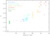 |
Fig. 1 Q-parameter (from our own photometry, Paper I) as a function of spectral type (from Bresolin et al. 2007). Different colors and symbols represent spectral types as indicated in the legend. Size indicates luminosity class (smallest symbols = class V, largest symbols = class I). The WO and the Be stars have been arbitrarily located in the X-axis. The Q color increases as we move towards later spectral types. Most stars with Q ≤ −0.4 are OB, Be, or WR stars. |
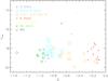 |
Fig. 2 Location in the Q vs. Vcorr diagram of the sample stars classified by Bresolin et al. (2007). Color and symbols have the same meaning as in Fig. 1. The different groups of stars (O types, B types, Be stars, and the WO) are located in separated loci of the diagram, with a small degree of mixing. |
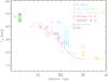 |
Fig. 3 Effective temperature derived from isochrone analysis as a function of spectral type. Colors and symbols have the same meaning as in Fig. 1 except for the magenta symbols. The latter represent the results on SMC stars by Mokiem et al. (2007) and Massey et al. (2009), and the calibration of Trundle et al. (2007) for B stars in this galaxy (lines; thick = supergiants, thin = dwarfs), derived from quantitative spectral analysis. The WO and the Be stars have been arbitrarily located in the X-axis. Dotted lines represent the revision of spectral types by Garcia et al. (2010, in prep.). Teff derived from isochrones for our IC 1613 sample increases with earlier spectral type as expected, but flattens at O stars, hinting that color degeneracy is still a problem for these types. The Teff we derived for the IC 1613 stars roughly agrees with the trend observed in the SMC. |
Figure 1 shows how Q partially breaks the color degeneracy of blue massive stars and is therefore useful for estimating stellar parameters. There is a strong correlation between the Q parameter (from our own Paper I photometry) and spectral type from the sample classified by Bresolin et al. (2007). Most stars with Q ≤ −0.4 have OB types. This was already shown in Fig. 5 of Paper I, where we also discussed the possible exceptions to this statement. While B-type stars exhibit a decreasing Q trend as we move towards earlier types, the trend flattens for O-stars with Q ≲ −0.90. Again, except for three B supergiants (out of 24), all targets with Q ≤ −0.90 are O or Be stars, or the only known Wolf-Rayet star in IC 1613 (WO 3 type; Kingsburgh & Barlow 1995).
In the Q vs. Vcorr diagram, we see that the different types (O, B, and Be stars, and the WO) are located in well defined loci with little mixing (see Fig. 2). The WO and Be stars populate a very blue region of the diagram, Be stars having typical Qs around –1.0. As we move towards increasing Q values, we find the few O stars of the sample of Bresolin et al. and three intruder early-B supergiants. However, examination of higher resolution spectra (to be presented in Garcia et al. 2010, in prep.) has led to the re-classification of some B0/1 supergiants included in both samples, to the O9 types. We therefore expect the bluest-Q stars of an association to be O stars and to match the youngest isochrone.
As a final test of the Q-based method, we evaluate the correlation of Teff rendered by isochrone analysis with spectral types. Fig. 3 shows that the evolutionary Teff increases towards earlier spectral types, as expected, and flattens for the O-types. There is a marked dispersion around B0-2 types, which is partly remedied after revision of some spectral types from our higher resolution spectra. We have also included in Fig. 3 the results of the quantitative spectroscopic analyses by Trundle et al. (2007), Mokiem et al. (2007), and Massey et al. (2009) for SMC stars (we excluded MW and LMC studies to avoid metallicity effects as much as possible). The temperatures derived by these works also exhibit some (if milder) dispersion, and experience flattening of Teff at O-types. Globally speaking, the trend in Teff derived from isochrones roughly agrees with the spectroscopic works, although it is systematically higher. The agreement improves with our revised spectral types, although some stars still deviate from the main trend. Figure 3 must not be taken as proof that we can determine accurately spectral subtypes and Teff for OB stars using the Q vs. Vcorr diagram. Figure 3 instead illustrates that the results from isochrone analysis are consistent with spectral types, with some [expected] dispersion.
We are therefore confident that our photometric-based study produces good first-order results, which are reliable in a statistical sense. However, our results for individual targets must be interpreted with caution. While we expect that the integrated properties of associations are reliable, a spectroscopic follow-up of individual members will be required to confirm their properties. However, doing so in an external galaxy is very expensive in observing time, and a list of the most massive candidates will be of great help.
2.2. Methodology
We studied the stellar population of the associations by comparing the color–magnitude diagram with theoretical isochrones, and estimated both their age and the mass of the members. We used the basic grid Z = 0.004 (0.2 Z⊙) isochrones provided by Lejeune & Schaerer (2001), who recalculated photometric colors for the stellar tracks of Charbonnel et al. (1993) using synthetic stellar spectra. Models with rotation were not used because evolutionary tracks for rotating stars have not been systematically published. In addition, vsini is not constant for the members of a given population, but exhibits a distribution that depends on the environment where the population formed (Wolff et al. 2007). The variation is seen galactic-wide (see the SMC for example, Trundle et al. 2007; Massey et al. 2009) but also in single OB associations (such as Cep OB2, Daflon et al. 2007).
Nevertheless, rotating and non-rotating tracks are very similar at the beginning of the main sequence, and we therefore expect that the use of non-rotating isochrones will have little impact on the results for the youngest associations. However, rotating models are more luminous at later stages of the main sequence, up to 0.5 mag at the end of the core hydrogen-burning stage (Maeder & Meynet 2003). As a consequence, stellar masses at that stage may have been overestimated. The impact on age determination is negligible given the intrinsic errors of this analysis.
As we explained in the previous section, we used the Q vs. Vcorr diagram to derive the physical properties of the OB associations. We used the unreddened V-magnitude of the targets to derive member ages and masses. The color–excess towards individual targets was calculated using the univocal relation between the Q parameter and the intrinsic colors of O and B stars (see Paper I and Sect. 2.1). According to our analysis in Paper I, this may introduce an error of 0.3 mag to the unreddened V-magnitude. The relation was parameterized for very low metallicity stars by Massey et al. (2000) (see Paper I, Eq. (3)). As far as we know, no similar relation exists for later spectral types; since the V-magnitudes of non-OB members of the associations could not be dereddened, they were not taken into account in the age determination. We used isochrones of log (t [years]) = 5.9,6.2,6.5,6.8,7.1,7.4,7.7,8.0, and 8.3 for comparison. The ±0.3 dex age intervals are adequate given the uncertainty in the location of the stars in the color–magnitude diagrams due to photometric errors (see the error bars in Fig. 4). Hence, the derived ages of OB associations have intrinsic errors of ± 0.3 dex.
We examined in parallel our INT-WFC images and complementary VLT-VIMOS images from program 078.D-0767 (Principal Investigator A. Herrero) to discard blends and background galaxies.
The global procedure is illustrated with an example association in Sect. 2.3, which includes general comments on the analysis. The color–magnitude and color–color diagrams of all the associations are published in the online version of the paper. Samples are shown in Figs. A.1–A.4. The derived physical properties of the associations are provided in Table 1. Neither background galaxies registered by our code nor OB associations that did not have at least three stars (labeled “Gal” and “d” in Paper I) are included here. Some parameters already presented in Paper I are repeated here for completeness.
2.3. An example: analysis of association #135
We consider the association #135 to illustrate the analysis performed on all the associations.
The color–magnitude diagram B−V vs. V of the association is shown in Fig. 4a. The isochrones have been shifted to account for the adopted distance modulus (DM = 24.27 Dolphin et al. 2001) and foreground extinction (E(B−V) = 0.02, Lee et al. 1993). These corrections were applied to the isochrones rather than to the stars to ensure that when using the diagrams to look for blue massive star candidates the user can estimate the apparent magnitude and color at a glance. Stars were classified as either likely OB or non-OB types according to the photometric criteria summarized in Tables 3 and 4 of Paper I; briefly, stars with Q ≤ −0.4 are candidate blue massive stars and stars with Q > −0.4 are all considered non-OB members. The OB stars of #135 are represented with blue circles in Fig. 4a, and non-OB stars with red circles. In the background, the catalog of all stars in IC 1613 with small photometric errors (see Paper I, Table 2) is drawn for reference.
The color–magnitude diagram displays a nice plume of young blue stars, with some dispersion at the base. This dispersion is normal and caused by a combination of effects: differential reddening, evolution away from the main sequence, projection effects, crowding, binarity, or a population that is not totally coeval. The stars are shifted from the isochrones, indicating that the reddening correction was insufficient and internal galactic reddening is at work. Two OB members have large B−V colors: the inspection of VIMOS images indicates that one of them is a blend (id: 60382) whereas the other one (id: 62813) appears to be isolated. These targets were not used for age determination. No other star shows blends except the second brightest star, and some targets with very blue Q color (see below). There is an additional population of 6 non-OB members, 3 of them in the region of red supergiants. The age of #135 cannot be determined from the B−V vs. V diagram because the isochrones overlap at the expected position of OB stars.
The isochrones and association members spread in the Q vs. Vcorr diagram (see Fig. 4b). In this plot, the isochrones have been shifted along the Y-axis to account for the DM, but no foreground extinction correction is applied. No correction is needed along the X-axis since, unless RV ≠ 3.1, Q is unaffected by reddening. The total (foreground and local) interstellar absorption towards each OB member was instead calculated using its Q parameter, and the subsequent correction (ΔV) was applied to the observed V-mag (Fig. 4b, diamonds). We note the larger error bars in Fig. 4b due to error propagation.
The bulk of OB members fall between the log age 6.8 and 7.1 isochrones, but there is a spread in age from log age 5.9 to 7.4. The spread in ages is seen in a large fraction of the catalog associations; we comment on this in Sect. 3. The brightest blue star is located close to the 6.8 isochrone. The red-supergiant candidates are consistent with log age 7.1−7.4, and the other red stars with 7.7–8.0; however, no reddening correction has been applied to their V-magnitude, so the objects may be intrinsically brighter. Other OB associations of our catalog also have log age = 8.0 red members (see for instance #122, #127, #147 ), which may be related to the uniform underlying distribution of older stars reported in IC 1613 (see references in Paper I).
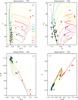 |
Fig. 4 Analysis of association #135, color–magnitude (top) and color–color (bottom) diagrams. Clockwise starting from top-left: a) B−V vs. V, b) Q vs. Vcorr, c) U−B vs. Q and d) B−V vs. U−B. The catalog of IC 1613 targets with good photometric quality is plotted with green dots. The likely OB stars of the association are the blue circles, and the non-OB members are represented in red. The error bars represent photometric errors. Diamonds in the Q vs. Vcorr diagram represent the OB members, their V-magnitude corrected for extinction (see Sect. 2.1). Note the larger error bars in this diagram, due to error propagation. In all panels except for the B−V vs. U−B diagram, colored lines represent the 0.2 Z⊙ isochrones of Lejeune & Schaerer (2001), whose log age is color–coded as indicated in panel a). In the B−V vs. U−B diagram, the dashed lines represent the reddening vector for O3–O9 stars. The other lines are the calibration of color with spectral type of Allen (2000) for O5-M5 main sequence stars (green), G5-M5 giants (blue), and O3-M5 supergiants (pink). |
The sequence of stars with very blue Q (~–1) was not used in the age and mass determination. Some of them seem to be blends or extended targets in the images, and are consequently discarded. The remaining stars with very blue Q were kept as valid members; we argue in Sect. 2.4 that these targets may represent various evolutionary stages of massive stars.
Figure 4c shows the plot of U−B vs. Q. All isochrones overlap in this diagram and mark the reddening-free position. The association points in this diagram have not been corrected for extinction in U−B. The #135 population is quasi-parallel to but offset from the isochrones, which once again is indicative of reddening. The spread in the alignment is evidence of some internal reddening.
Finally, Fig. 4d helps us to readily identify the cases of anomalous reddening, which are likely to correspond to a misleading Q color and require further investigation. These cases were not automatically discarded, since they may contain massive stars in interesting advanced stages (see for instance the location of IC 1613’s LBVc and WR). In association #135, star 60382 (B−V ~ 0.3, U−B ~ −0.7) sits in a locus usually populated by intruders, targets that entered our catalog because of their bluish Q but are actually red objects, in most cases blends or background galaxies. Visual inspection usually suffices to identify these cases. The other kind of intruders are those with Q ~ −0.4. As pointed out in Paper I, the relation between Q and spectral type is no longer univocal for Q > −0.4. The combination of the non-monotonic behaviour of the function at spectral types later than B9 and photometric errors (see Sect. 5.1.1 of Paper I) may result in F and G stars having Q ~ −0.4. This could be the case for 62813 with B−V ~0.5; we note, however, that this star follows the reddening vector, its position being consistent with that of a very reddened OB star. Spectroscopy is the only way to confirm beyond doubt that the members are massive stars, or otherwise.
2.4. Very blue Q members
We often encountered bluer targets than the bluest isochrone points in the Q vs. Vcorr diagram, as we found for association #135. Visual inspection indicates that some of these targets are blends, but a large number of apparently isolated stars display very negative Q colors. Since some of them are found in regions with nebulosity, we explore in this section whether nebular contamination can produce very blue Q colors.
Expected Q color changes (Qneb, ∗ −Q ∗ ) due to nebular contamination as a function of spectral type.
The change experienced by magnitude because of nebular contamination can be written
![Mathematical equation: \begin{eqnarray} \label{eq:1} m_{\rm neb,*}-m_{*} \,& = \, & -2.5 \log \left[ 1+ \frac{\int {\rm Filter} \cdot F_{\rm neb}(\lambda) \, {\rm d} \lambda}{\int {\rm Filter} \cdot F_{*}(\lambda) \, {\rm d} \lambda} \right], \end{eqnarray}](/articles/aa/full_html/2010/15/aa15243-10/aa15243-10-eq45.png) (1)where
m∗ and
mneb, ∗ are the stellar and
stellar+nebular magnitudes, Fneb(λ) is the
flux of the nebular line, and F∗ is the stellar flux. If we
approximate Fneb(λ) by a Dirac-Delta function
containing all the flux of the nebular line, Eq. (1) now reads
(1)where
m∗ and
mneb, ∗ are the stellar and
stellar+nebular magnitudes, Fneb(λ) is the
flux of the nebular line, and F∗ is the stellar flux. If we
approximate Fneb(λ) by a Dirac-Delta function
containing all the flux of the nebular line, Eq. (1) now reads ![Mathematical equation: \begin{eqnarray} \label{eq:2} m_{\rm neb,*}-m_{*} = -2.5 \log \left[ 1+ \frac{ F_{{\rm neb},w} }{10^{-0.4 \, (m_{*}-C)}} \right], \end{eqnarray}](/articles/aa/full_html/2010/15/aa15243-10/aa15243-10-eq50.png) (2)where
C is the photometric calibration constant and
Fneb,w the nebular flux weighted by the
filter transmissivity.
(2)where
C is the photometric calibration constant and
Fneb,w the nebular flux weighted by the
filter transmissivity.
We used the observed fluxes provided by Lee et al. (2003) for all the detected nebular lines of Hodge et al. (1990)’s HII region #13 in IC 1613, and calculated their contribution to the UBV filters. We simulated the Q color change (ΔQ = Qneb, ∗−Q ∗ ) for O4 and O9.5 stars of luminosity Classes I and V (see Table 2). Intrinsic colors were taken from the calibration of Martins & Plez (2006), and corrected for IC 1613 foreground extinction. The variations listed in Table 2 amount to a maximum of ΔQ ~ 0.02 for O stars, and cannot explain the very blue colors we find in the Q vs. Vcorr diagram of some associations, which would require ΔQ < −0.3 in some cases. The simulated change is larger (ΔQ ~ −0.15) for B0 I stars (intrinsic colors from Massey 1998).
The HII region #13 is relatively cold (Te,O + 2 < 14540 K) and of low density (ne = 100 cm-3), which may explain the small simulated Q variations. No other absolute line fluxes are available for IC 1613 HII regions except for Hodge et al. (1990)’s #37, the nebula ionized by the Wolf-Rayet star of the galaxy. While still of low density, this nebula is hotter (Te,O + 2 = 17910 K). O stars embedded in this nebula would exhibit bluer Q color (ΔQ ~ −0.02) than if located in a region free of ionized hydrogen, except for the O9.5 V type (ΔQ ~ 0.16). Again, the variations would be larger for B0 stars.
These figures indicate that it is difficult to quantify the extent to which the nebular lines affect the stellar colors, with shifts in the Q axis working in both directions. The nebular electronic temperature, density, chemical composition, and the stellar continuum, all play important roles. However, even when a strong HII region is present, the induced ΔQs remain modest, unable to explain the most extreme cases of blue Q.
What are the other possible explanations of the very blue Q sources, if nebulosity is not their likely origin? There is a metallicity dependence in the evolutionary models, such that metal-poorer isochrones display bluer Q colors. We verified that within the uncertainties in the chemical abundances derived for IC 1613, the corresponding Q variation (ABS(ΔQ) < 0.1) cannot account for very-blue Q stars. Moreover, this would not be consistent with a regular chemical enrichment of the galaxy, where young OB stars would be the metal-richest. The Q color may also have been underestimated in the areas of anomalous reddening slope; however, this cannot be characterized without spectroscopy or multiband photometry extending towards the infrared. The color combination of close stars (either projected targets or real binary systems) may yield a blue Q color, but their detection is beyond currently available observations. Extremely-blue Q objects may also be hot planetary nebulae (hotter than the HII regions powered by OB stars), but only 10 PN are expected in IC 1613 and only 2 have been found (Magrini et al. 2005).
Finally, very blue Q objects can represent different evolutionary stages of massive stars than the OB types. We showed in Sect. 2.1 that Be stars are located in the bluest region of the Q vs. Vcorr diagram, with Q ≲ −1.0. The Wolf-Rayet star in IC 1613 has Q ~ −1.35 (see Paper I); in this case, the intrinsic color of the advanced phase may add to the contamination of the hot surrounding nebula. Hence, we do not discard very blue Q targets as association members, although they are usually farther from the isochrones than the error bars and therefore cannot be used for association age and mass determination. Nonetheless, a spectroscopic follow-up to unveil the true nature of very blue Q sources would be highly interesting.
3. Results: Physical properties of the OB associations
3.1. Size
The interest in finding a typical size-scale for OB associations is that it relates to the mass of the parent cloud and the scale of molecular cloud instabilities. Star formation in galactic disks was proposed in the past to have a universal lengthscale of approximately 80 pc (Efremov et al. 1987; Ivanov 1991). The resulting populations would then nest into larger systems (Efremov et al. 1987) of size ~0.2 kpc (aggregate), ~0.6 kpc (complex) and ~1.2 kpc (supercomplex). As we explained in Sect. 2, this picture is changing, star formation now being viewed as a hierarchical process producing groups of stars enclosed within each group of stars and so forth, and the derived typical sizes of OB associations being a result of definition. In this section, we check whether our results agree with the traditionally accepted typical size, when following a traditional definition of OB association.
We use the radius of the circle that circumscribes a given association as the indicator of its size. Even though this indicator is inadequate for linear associations and introduces scatter in the statistics, it clearly represents the association dimensions. Most of the groups found have a radius of 6″ or smaller (see Fig. 5). The average size is 6.1″ with a large standard deviation of 4.5″. At the adopted distance modulus of DM = 24.27, the size of 1″ corresponds to 3.5 pc, hence our associations have an average 42.7 pc diameter. There is a marked peak of radius 2″–6″, corresponding to diameters of 14 pc–42 pc. When only associations with 4 elements or more are considered, the size distribution does not change at its long end (R = 6″ or larger, Fig. 5). However, the number of small associations decreases drastically, indicating that the average size is shifted towards smaller values by the groups of three members. The distribution now peaks at 4–7″ with an average diameter of 59 pc.
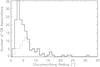 |
Fig. 5 Size distribution of the associations listed in our catalog (solid line), all having a minimum of 3 good members. The mean size is 6.1″ ± 4.5″, and the distribution peaks at 2–6″. The dotted line is the distribution of associations with 4 elements or more. The number of small associations decreases drastically, but for R > 6″ the function remains unchanged. |
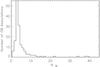 |
Fig. 6 Distribution of the population. To use a convenient scale, association #151 with 69 candidate OB stars was not included in this plot. Besides #151, 4 associations are well populated with more than 20 members. However, most of the groups have 10 or fewer members; a population of 3 OB stars is the most common. |
A size of 40 pc is half the suggested typical length scale of OB associations, 80 pc. Our analysis would only match this figure if we considered 5 OB stars as the smallest group. Notwithstanding, we would detect no more than 3 or 4 members for some typical Galactic OB associations if located at the distance of IC 1613, as we argued in Paper I. Additional instrumental effects that may be at work are discussed in Appendix B. We appear to detect more elementary sub-groups than traditional OB associations.
One possible explanation of this is that our algorithm detects the denser cores of classical OB associations. Substructure had already been found in early catalogs of associations made by eye (Blaauw 1964), but also by Bresolin et al. (1998) and Pietrzyński et al. (2001, 2005), who both find that associations larger than 200 pc can be separated into smaller denser groups. We only find one association of roughly 200 pc in diameter, #151, and visual inspection indeed reveals that it could be broken into smaller pieces of high density. Additional associations of radius larger than 20″ (i.e. diameter > 140 pc) are also large groups of the bubble region (#127, #137, #147) and all display structure. The associations #127 and #137 have a concentration of central brighter stars with fainter members farther from the center, following several arc-like structures. In a similar way, the stars of #147 follow the nebular distribution, but several bright cores are seen.
Another possible reason for the smaller size of our associations is the requirement of very accurate U-band photometry of the members (see Paper I). As the error increases rapidly with decreasing apparent magnitude, stars that would have been included because of their blue B−V colors (like late-B stars or even hot subdwarfs) are excluded. A smaller number of members leads to the inference of a smaller association radius.
3.2. Population
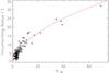 |
Fig. 7 Size of the associations as a function of the number of OB stars (crosses). As expected, size increases with increasing number of members. The solid line represents the least squares fit to the points: NOB = 0.04 + 0.32 ∗ R + 0.05 ∗ R2. |
The typical population of the associations in our catalog is less than 10 members (see the distribution in Fig. 6). We only considered stars checked against blends when evaluating this number. Approximately half of the total (44%) are small associations with 3 members. We find that 21% have 4 members and 34% have a minimum of 5. A significant 10% have more than 10 OB members.
The size of the groups increases with the number of OB members (see Fig. 7), with a smooth behaviour that can be fitted by the paraboloid NOB = 0.04 + 0.32 × R + 0.05 × R2. Although some scatter is seen in Fig. 7, there are no important deviations from the general trend. This implies that globally speaking the population of blue massive stars in IC 1613 exhibits no region of over-density.
3.3. Stellar masses and environment
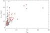 |
Fig. 8 The mass of the most massive star of each association is plotted as a function of the number of bona fide OB members (black symbols). Red diamonds represent the average Mup of all associations with the same number of members, their error bars being the standard deviation. The general trend is that Mup increases with the number of members. Note however that some poorly populated associations (3-5 members) also have very high upper masses, as in the case of Orion’s Trapezium. The most populated association, #151 with 69 members, deviates from the main trend. |
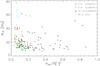 |
Fig. 9 The mass of the most massive star of each association is plotted as a function of stellar density, estimated as the number of bona fide OB members divided by the squared radius of the association. Different symbols represent NOB, as indicated in the legend. Associations #94 and #184 with density 1.2 and 1.9 are left out of the plot for clarity. |
The initial and current mass of the most massive member of each association is registered in Table 1. These figures are obtained from the position of the star in the Q vs. Vcorr diagram, using the unreddened V-magnitude (see Sect. 2.3). We analyze in Fig. 8 whether there is a correlation between the current mass of the most massive member of an association (Mup) and the number of bona fide OB members (with regular Q-parameter, no blends). Well-populated associations contain very massive stars, as expected for a regular IMF. If we consider the averaged Mup of all associations with the same number of elements, we discern a trend of larger Mup in more populated associations. Notwithstanding, some scarcely populated associations with 3 to 5 members also have large Mup. One obvious explanation is that in these cases the faintest members exist but were not detected, not included in the catalog because of their photometric errors, or obscured beyond detection by extinction. Another possibility is that the most massive member is actually multiple. In addition, the catalog of associations was generated automatically and their physical identity cannot be assured; as a consequence, NOB could be different, shifting the association in the X-axis of Fig. 8. Alternatively, these may be cases of poorly sampled IMF as happens in our own Galaxy in the Orion Trapezium cluster, consisting of an O7 V plus three B0.5 V stars.
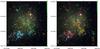 |
Fig. 10 Ages of OB associations in IC 1613. North is left and east is down. The association perimeters are plotted over the INT-WFC RGB image of IC 1613 (same field shown as in Fig. 9 of Paper I), with the age indicated by the contour colors. Since most associations exhibit age dispersion, the left panel shows the age of the youngest association members, and the right panel the age of the older members. Color–code is: cyan log age = 5.9, blue log age = 6.2, dark green log age = 6.5, light green log age = 6.8, yellow log age = 7.1, orange log age = 7.4, red log age = 7.7, violet log age = 8.0. The largest concentration of young associations is found in the bubble region of the galaxy in the NE lobe. |
The most populated association (#151, NOB=69) does not follow the main trend. In contrast, its upper blue color–magnitude diagram is very well populated with 4 blue massive stars (two of them confirmed spectroscopically) plus one star that could be contaminated by a nearby object. There is also a large number of targets in the region of Q-color bluer than the isochrones. As we explained before, they were not used in our Mup determination; we note, however, that WR and Be stars could be located in this region of the Q vs. Vcorr diagram, hence we may be missing “exotic” evolutionary stages for the mass budget. In addition, #151 encloses the only known SNR of IC 1613, which most likely formed in a type-II supernova (Peimbert et al. 1988). However, according to the theoretical predictions the mass of the progenitor ranges from 8 to 54 M⊙ (Georgy et al. 2009), still rendering #151 below the main trend of Fig. 8.
Enhanced extinction expected in this area rich in HI and HII may have also led to an underestimation of Mup. We also note that #151 shows some sub-structure. If #151 were separated into smaller pieces, one of them containing the current most massive member, the association would follow the main trend. This example illustrates the uncertainties involved in deriving evolutionary masses, and why a more thorough analysis, including spectroscopic data, is needed before drawing any strong conclusion about the IMF of any of the associations.
The most massive stars are not found in environments of high stellar density (represented by the ratio of NOB to the squared radius) as we show in Fig. 9. The combination of Figs. 8 and 9 hints that it is the total number of members (i.e., the total mass of the association), rather than their concentration, that constrains Mup.
3.4. Total association mass
We used the Salpeter initial mass function to calculate the total mass of the OB associations of the catalog. The results must be taken as a rough estimate, since our study can neither ensure membership of the targets, nor take into account the incompleteness of our photometry at the faintest end of the color–magnitude diagram. In addition, the IMF is not straight but its slope changes at certain stellar masses (whose value vary in the literature), and may also depend on metallicity (see review by Kroupa & Weidner 2005). Since a detailed account of the mass enclosed in the OB associations of IC 1613 is beyond the scope of this paper, we approximated a constant slope of α = 2.35.
In the power-law form of the initial mass function, the number of stars with masses in
the interval
[M1,M2] of
a population can be expressed  (3)and the total mass
enclosed in the same
[M1,M2]
interval
(3)and the total mass
enclosed in the same
[M1,M2]
interval  (4)We used
Eq. (3) and the member masses produced by
our analysis to estimate the IMF constant 𝒞. Since we applied no completeness
correction to the faintest members, only OB candidates were considered for the calculation
(except identified blends and very blue Q objects). We used the maximum
mass of the association Mup to represent M2, and
M1 was set to be the lowest mass of the lists of remaining
members with
M > 12 M⊙. In
some small associations, this list contains only one or even no stars; in these cases,
M1 was set to the minimum association mass. After
𝒞 was determined, we integrated the total
association mass from 0.5 M⊙ to
Mup using Eq. (4). The results are listed in Table 1.
(4)We used
Eq. (3) and the member masses produced by
our analysis to estimate the IMF constant 𝒞. Since we applied no completeness
correction to the faintest members, only OB candidates were considered for the calculation
(except identified blends and very blue Q objects). We used the maximum
mass of the association Mup to represent M2, and
M1 was set to be the lowest mass of the lists of remaining
members with
M > 12 M⊙. In
some small associations, this list contains only one or even no stars; in these cases,
M1 was set to the minimum association mass. After
𝒞 was determined, we integrated the total
association mass from 0.5 M⊙ to
Mup using Eq. (4). The results are listed in Table 1.
As we explained in the previous section, we suspect that the IMF of the associations in our catalog is poorly sampled. As a consequence, M2 and M1 may be very close values, and produce an artificially large constant 𝒞. This can physically be interpreted as degeneracy, an attempt to use two bins that are too close to constrain the IMF. To avoid this effect as much as possible, mass errors were also taken into account, but the total masses derived for poorly populated associations must be interpreted with caution.
The masses we found for the associations range from 1.1 × 10² M⊙ to 5.1 × 10³ M⊙, with an average (5.0 ± 5.4) × 102 M⊙.
3.5. Association ages
This work has rendered ages for the OB associations of IC 1613 ranging from log age = 5.9 to 7.7, usually with some spread. We study their spatial distribution in Fig. 10. As expected, the associations with the youngest age considered (log age = 5.9) are concentrated in the bubble region of the galaxy, the NE lobe, where spectacular giant HII shells are seen (Meaburn et al. 1988; Valdez-Gutiérrez et al. 2001). Additional young associations are also common on the SW bank of the HI-cavity that separates the IC 1613’s optically brightest area into two (see Fig. 11), but the average is shifted to slightly older ages of log age = 6.5–6.8. In both areas, the youngest associations tend to cluster: it is unusual to find isolated associations of log age = 6.5 or 6.8. There seems to be a galactic-scale age gradient in the NE direction, with the youngest members being in the NE lobe. Finally, there is a number of isolated associations far from the central stellar concentrations (mainly in the south and western outskirts). Some of them have members as young as log age = 5.9, which is unexpected, since they are far from the bubble region, the traditionally assumed locus of intense star formation.
The age spread is smaller on the SW bank of the HI hole, where the typical maximum age is log age = 7.4. Older stars (log age = 7.7) are found in the associations with the youngest population in the bubble region (#137, #147, #151). Since this area is rich in hydrogen (see Sect. 4.1), the age spread may be the product of ongoing star formation. However, this could also be an artifact of dust: an anomalous steeper reddening-law would send stars to the red region of the Q vs. Vcorr diagram and bias the analysis towards higher ages. Dust detection by IRAS and Spitzer in the bubble region (Meaburn et al. 1988; Jackson et al. 2006) support this hypothesis. The determination of spectral types and spectroscopic reddening would settle the question, but is left to a future paper. Another plausible explanation of the large age dispersion in the bubble region is that we observe populations at different depths in our line of sight; a kinematic study would help us distinguish the different projected populations.
3.6. Comparison with previous works
Georgiev et al. (1999) present the most recent study of the OB population of IC 1613. They analyzed the color–magnitude diagrams of Hodge (1978)’s associations in the bubble region of IC 1613 to derive ages and Mup. Their results are summarized in Table 3, together with data from our counterpart associations. A direct cross-match of both catalogs is not straightforward (as we discuss in Paper I), with the additional problem that some Hodge (1978)’s associations enclose more than one association of our catalog. In these cases, the age-range listed under “This work” encloses the ages of all the included associations, Mup being the maximum of all of them.
The ages derived by Georgiev et al. (1999) are always included in the interval we provided for our counterpart association(s), usually close to the lower limit. The age derived by Georgiev et al. (1999) for #161, the exception to this statement, differs from our lowest value by 5 Myr. Our derived ages extend to older values. The likely explanation is our selection criteria for OB stars, which is more relaxed in V and B−V. Whether the fainter targets are coeval reddened members or actually belong to an older population needs to be established by future work involving spectroscopy.
In terms of the uncertainties in deriving evolutionary masses, both works roughly agree except for association #161, which includes some targets with a very blue Q color for which we could not determine masses. Associations #161 and [H78]17 also do not fully match, the latter having a larger number of members. The different Mup could also be an association identification issue.
Ages and Mup found for the associations: comparison with Georgiev et al. (1999) results.
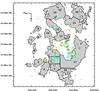 |
Fig. 11 Relative distribution of neutral hydrogen and OB associations. The grey shadow outlines the distribution of HI in IC 1613 (adapted from Fig. 1 of Silich et al. 2006). Colored contours indicate the position of the associations of Garcia et al. (2009). Color indicates the age of the youngest members, with the same color code as in Fig. 10. Numbers follow the HI fragment numbering of Silich et al. (2006). The HI cavity is surrounded by fragments 1, 10, 11, 14, and 17. |
4. The interplay of gas and stars
4.1. Associations and neutral gas
The distribution of the OB associations of IC 1613 can be explained by comparing it with the observations of neutral hydrogen from the Very Large Array at NRAO (Silich et al. 2006). Inspection of Fig. 11 reveals five relative dispositions of gas and young stars. The distribution of HII (Valdez-Gutiérrez et al. (2001)’s catalog, for instance) relative to neutral hydrogen follows a similar pattern as OB stars.
Current mass of the most massive stars in IC 1613.
-
1
Associations whose projected position matches that of highmasses of neutral hydrogen: The largest OB associations ofGarcia et al. (2009) are found inSilich et al. (2006) HIsegments 1 (assocs. #127 and #137) and 2 (#147and #151). They are located in the active star-forming NE regionof the galaxy, where the highest concentrations of neutralhydrogen are also found (Silichet al. 2006). Since there is a largehydrogen reservoir, star formation may still be at work,explaining the wide age spread seen in this region.
-
2
Associations located inside the HI void: There is no neutral hydrogen on the SW edge of the HI cavity which, in turn, is rich in associations. In this region, all hydrogen must have been ionized. In fact, Valdez-Gutiérrez et al. (2001)’s R14, R15, R16 and R17 HII regions overlap with the associations. A similar scenario has been proposed for WLM, where the neutral hydrogen appears to have been consumed or ionized by star formation (Kepley et al. 2007). A smaller initial amount of HI in this area than in fragments 1 and 2 would explain the present-day lack of hydrogen, and the smaller age spread seen in this region. The origin of the HI cavity remains unknown. Silich et al. (2006) concluded that the multiple SNe scenario could not provide an explanation. Hydrogen exhaustion by star formation seems a plausible explanation, or at least, a contributing factor.
-
3
Associations on the walls of HI shells: Far away from the traditionally considered loci of current star formation in IC 1613, we also find associations with very young members: #17, #83, and #142 on the southern side, and on the west side #3, #5, #6, #8, #12, #13,#15, #18, and the #16-#19-#21-#22 complex. IC 1613’s HI distribution extends beyond the HI-hole, and forms additional HI cavities and arc-like structures (Lozinskaya et al. 2001; Silich et al. 2006) where the listed associations are located (see Fig. 11).
-
4
Associations inside HI shells: Association #142, apparently isolated, is located inside a hole in the middle of HI fragment 17. This association may have consumed all the HI gas in its vicinity or produced the hole by radiation pressure. It is possible that additional associations are hidden behind the HI; however, the density is low as confirmed by the background galaxies seen. In the bubble region, we find Lozinskaya et al. (2003)’s neutral hydrogen shells II and III, which have kinematical ages 5.3–5.6 Myr, i.e., log age = ~6.7. OB associations in this area span an age interval of log age = 5.9 to 7.4–7.7, hence are consistent with the hypothesis that OB stars have blown these shells.
-
5
Finally, our algorithm did not find any (or very few) OB associations in the outer hydrogen ring of the galaxy corresponding to HI fragments 4–9, 13, and 15–18, although isolated blue stars are seen. The neutral hydrogen density is lower in this region, which may explain the poorer production of massive stars. This suggests that the typical lengthscale of OB associations or clusters found by automatic methods should correlate with the neutral hydrogen density, because of the dependence of stellar density on this parameter.
4.2. Local induced star formation
Except for the NE lobe of IC 1613, OB associations and HII regions are mostly concentrated at the edges of high HI masses. Hodge et al. (1990) pointed out that this disposition of ionized relative to neutral hydrogen resembles the patterns seen in our Galaxy, where some hydrogen clouds display star formation concentrated near the edges. In the context of Elmegreen & Lada (1977)’s work, this may be a signature of sequential star formation of OB stars in a large molecular cloud. These authors calculated that the new stars formed between the ionizing and shock fronts originating in a group of OB stars and propagating into the molecular cloud, are likely to be more massive than the stars formed in unshocked faraway regions of the cloud. In this scenario, given a large molecular cloud, OB stars would form in a spatial and temporal sequence of bursts. Further refinement of the age determination of the youngest population of IC 1613 would be important to test this hypothesis. However, this is not possible without spectroscopic information.
The brightest stars of IC 1613 and the most populated associations are located at the boundaries of the HII shells and the intersection of different bubbles. Lozinskaya et al. (2002) studied whether the collision of expanding HII shells (driven by the combined winds of central OB stars) with the neutral hydrogen could induce star formation. HI and HII actually interact along the lines defined by arc-like distributed stars (Lozinskaya et al. 2003) in the bubble-rich region of IC 1613. They concluded that the bubble rims represent the most active star-forming region of the galaxy.
Some of the associations of our catalog have members at both the rim and the center of an HII region. We did not find different ages for center vs. rim members, in apparent contradiction with the proposal that they have different formation mechanisms. However, spectroscopy is needed to confirm this result.
The collision of expanding HI shells may also produce gravitational instability and star formation (Valdez-Gutiérrez et al. 2001; Lozinskaya et al. 2002; Efremov 2002), possibly forming the outer OB associations of the galaxy.
5. Stellar masses
5.1. The most massive stars of IC 1613
Table 4 is a compilation of the heavy-weights of IC 1613: stars enclosed in associations, with current estimated mass M ≥ 50 M⊙. To calculate the error bars, we estimated the mass of each star at the 8 positions of the square defined by the photometric errors; the error bar represents the maximum of the absolute difference of these values from the central stellar mass. Hence, they account only for the photometric errors, and do not attempt to simulate the intrinsic errors in the method.
There are 13 stars more massive than 50 M⊙, which are distributed in eleven associations. Except for associations #43 and #120, all are located in the NE complex. We note that Table 4 is not a complete census of very massive stars in IC 1613, since only stars in associations were considered when compiling this list. Stars with Q color bluer than the isochrones beyond the errors were also discarded for Mup determination, but may have high initial masses (as is the case for the WO of the galaxy). Most of the Be stars in IC 1613 could also be left out of Table 4.
Three groups of stars can be distinguised in Table 4: bright stars (V < 19), young faint stars (log age ~6.2) and 57798, which has a large reddening correction. One would likely have suspected that 62 390, 59 802, 34 964, 69 336, and 60 449 were very massive, as they are blue and belong to the group of eleven brightest stars of IC 1613 (see Paper I). However, stars with (V > 19) would likely have been missed in a survey to detect the most massive members of the galaxy. Nonetheless, it is encouraging that, when spectral types are known, the stars of the highest masses according to this photometric-based study correspond to spectral types OBA, even for the fainter objects.
We now examine a case of large V-magnitude reddening correction: 57 798 (ΔV = −2.65). The star belongs to association #120, which also hosts 58040, a B2 Iab star (see Table 1 and Paper I). The targets are only 2.5″ away, have very similar Q colors (–0.74 and –0.82), and look point-like in the images. The star 57 798 (B−V = 0.62, U−B = −0.29) is remarkably more reddened than 58 040 (B−V = −0.09, U−B = −0.88). The R-band VIMOS images of 57 798 appear to display nebulosity around this object but not conclusively. A similar case of very high local reddening (E(B−V) ~ 0.5) was found and spectroscopically confirmed for the LBVc V39 (see Herrero et al. 2010); the colors of 57 798 are also remarkably similar to those of V39 (B−V = 0.62, U−B = −0.19, Q = −0.636). Spectroscopic follow-up is planned to determine the true nature of 57 798.
5.2. Mass discrepancy in IC 1613?
The disagreement between evolutionary and spectroscopic masses of OB stars is a long-standing problem, already reported by Herrero et al. (1992). The difference was partly reconciled when a more detailed description of the OB star atmospheres was used to derive the spectroscopic masses (Herrero et al. 2002; Repolust et al. 2004) or when other factors such as He abundance were taken into account (see the review by Puls (2008)). However, the discrepancy remains for some Galactic B-type supergiants (Markova & Puls 2008) and some OB stars in the metal-poor LMC and SMC (Massey et al. 2009). This work enables the first evaluation of the mass discrepancy in a very metal-poor environment.
In Table 5, we compare the mass derived in this work (evolutionary mass) with the mass of 7 OB supergiants estimated by Bresolin et al. (2007) from their quantitative spectroscopic analysis of FORS data (spectroscopic mass). The difference is larger than (but on the order of) that found by Massey et al. (2009). The evolutionary masses are a factor of 2 to 3 higher than the spectroscopic masses, except for one of the targets. Our error bars for the evolutionary masses cannot explain the difference. The most remarkable case in Table 5 is 60 449, with a five-fold difference between spectroscopic and evolutionary mass. Bresolin et al. (2007) found no pecularity regarding this star. Their provided V-magnitude is the same as in the catalog of Garcia et al. (2009), thus discarding the occurrence of an outburst. The high mass derived in this work may be caused by the Q-color based extinction correction, which amounts to –0.5 mag in V.
Spectroscopic masses (Bresolin et al. 2007) vs. evolutionary masses (this work) for OB supergiants in associations.
The reddening correction has an obvious impact on our results. We reported in Paper I that the values we derived for the color excess E(B−V) are systematically larger than Bresolin et al. (2007)’s, implying a larger correction in V. The reddening correction may therefore explain the higher evolutionary masses for some targets. However, the color excess we derive for 67 841 roughly agrees with that of Bresolin et al. (2007). Yet its evolutionary mass is still twice as high as its spectroscopic mass, implying that extinction is not the only factor at work. If we correct 67 841’s V-magnitude using the spectroscopic reddening correction and calculate its mass, the discrepancy is far from being reconciled (we now obtain Mevol = 27 M⊙). Bresolin et al. (2007) warn that their spectroscopic masses are a lower limit, since stellar rotation could not be accounted for properly in their study. In contrast, the evolutionary masses may have been overestimated since we used non-rotating isochrones. Additional quantitative analysis of higher resolution spectra are needed before any definite conclusion about the mass discrepancy can be drawn.
6. Summary
We have presented and discussed the physical properties of the catalog of IC 1613 associations produced by our automatic search code (Garcia et al. 2009). Even though the listed groups of stars cannot be proven to be meaningful physical entities either because of the underlying philosophy of the method, or because the concept of OB association has changed, it is a necessary first step in studying the population of young massive stars.
Our work here has involved the examination of images, and both color–magnitude and color–color diagrams for all populations, to identify blends and outliers in the reddening plot, while deriving ages and masses for the members. A useful tool, we found, is the Q vs. Vcorr diagram, where isochrones are clearly separated and colors are free from reddening. While this method is affected by important drawbacks, such as the failure of the Q parameter in non-standard reddening environments, the traditionally used B−V vs. V diagram is not free from them either. The smaller amount of degeneracy in the Q color (compared to B−V) of massive stars, and the agreement of our results with previous works (traditional population analysis of OB associations and available spectroscopy for some members), support the use of the Q vs. Vcorr diagram for young population analysis.
The associations concentrate in the bubble NE region of the galaxy, with members being as young as log age = 5.9. In this area, old members (log age = 7.7) are also seen. The spread in age suggests that star formation is ongoing to the present day; this is consistent with the large concentration of neutral hydrogen in the area. Young associations are also seen on the SW edge of the HI cavity, where the average younger members have log age = 6.8, but the age spread is smaller. Hardly any neutral hydrogen is seen in this area.
We have found that the mass of the most massive member usually increases with the number of OB members. However, very massive stars are also found in scarcely populated associations. While these findings may be caused by the systematics of the present study, we may be witnessing a poorly sampled IMF as is the case in the Galactic Trapezium cluster.
The average size of the associations in this catalog is 40 pc, half the traditionally considered typical lengthscale. There is a strong correlation between size and number of members.
Our procedure has proven very effective in finding massive stars, with existing spectroscopic confirmation for some of them. The evolutionary masses derived in this work are systematically higher than the spectroscopic masses that Bresolin et al. (2007) derived for the same objects. Extinction (while often overlooked) may exacerbate the disagreement between mass measurements. However, the discrepancy persists for at least one object for which both Bresolin et al. (2007) and this work derive similar E(B−V) values.
The final goal of the study presented in this paper was to produce a list of interesting candidate OB stars either because they are young, massive, and embedded in a dense environment or because they may be in an advanced stage of evolution. It is our immediate intention to perform a spectroscopic follow-up of these candidates.
Online material
Properties of OB associations.
Appendix A: Color–magnitude and color–color diagrams of the associations
 |
Fig. A.1 Color–magnitude diagrams of all groups listed in Garcia et al. (2009)’s catalog. Green dots in the background represent the complete list of targets with good photometric quality data in IC 1613. Blue circles represent the OB candidate stars of the associations, and red circles other members. Lejeune & Schaerer (2001)’s 0.2 Z⊙ isochrones are included for reference, shifted to account for distance (DM = 24.27) and foreground reddening E(B−V) = 0.02. Different colors represent different log age, as indicated in the legend. |
 |
Fig. A.1 continued. |
 |
Fig. A.1 continued. |
 |
Fig. A.1 continued. |
 |
Fig. A.1 continued. |
 |
Fig. A.1 continued. |
 |
Fig. A.1 continued. |
 |
Fig. A.2 Q vs. Vcorr color–magnitude diagrams of all groups listed in Garcia et al. (2009). Colored lines represent the theoretical isochrones with the same age code as in Fig. A.1, shifted by the DM, but without any correction for foreground extinction. Black diamonds represent V-magnitudes of the blue members, corrected from total extinction (foreground and local). Red circles represent the red members. These diagrams were used for age and mass determinations. |
 |
Fig. A.2 continued. |
 |
Fig. A.2 continued. |
 |
Fig. A.2 continued. |
 |
Fig. A.2 continued. |
 |
Fig. A.2 continued. |
 |
Fig. A.2 continued. |
 |
Fig. A.3 U−B vs. Q color–color diagrams of the associations, using the same color code as in Fig. A.1. Theoretical isochrones are included for reference. Since no extinction correction was applied, the lines mark the locus of an unreddened population. A population parallel to the isochrones but shifted indicates reddening. Note that the isochrones of all ages overlap. This provides further supporting evidence for the selection criteria (Q < −0.4) to find candidate blue massive stars used in Garcia et al. (2009). |
 |
Fig. A.3 continued. |
 |
Fig. A.3 continued. |
 |
Fig. A.3 continued. |
 |
Fig. A.3 continued. |
 |
Fig. A.3 continued. |
 |
Fig. A.3 continued. |
 |
Fig. A.4 B−V vs. U−B color–color diagrams. Color codes for points are the same as in Fig. A.1. The red line indicates the reddening vector for O3-O9 stars. The other lines are the calibration of color with spectral type of Allen (2000) for O5-M5 main sequence stars (green), G5-M5 giants (blue) and O3-M5 supergiants (pink). |
 |
Fig. A.4 continued. |
 |
Fig. A.4 continued. |
 |
Fig. A.4 continued. |
 |
Fig. A.4 continued. |
 |
Fig. A.4 continued. |
 |
Fig. A.4 continued. |
Appendix B: On the systematics of automatic methods to build OB association catalogs
In this work, we have found an average size of OB associations of ~40 pc, with the peak of the distribution ranging from 14 pc to 42 pc. This figure is half the universal size of associations proposed by Efremov et al. (1987) and Ivanov (1991): 80 pc. The accepted paradigm of massive star formation is evolving and the concept of OB association is changing to that of a scale-free global distribution, hence the concept of universal size is now meaningless. However, it is reasonable to expect that objective automatic methods following the same philosophy of searching for OB clusterings would lead to similar results. Ivanov (1996) found an average size of roughly 80 pc from the average of an heterogenous set of data including IC 1613, other irregular galaxies (NGC 6822, Pegasus, Sextans A, GR 8, Ho IX) and nearby spirals (M 31, M 33). Bresolin et al. (1998) analyzed HST-WFPC2 data for 7 spirals, and found the same value. Bresolin et al. (1996) finds very similar association size distributions in LMC, SMC, M 33, NGC 6822, and M 101, with a peak in the range 40–80 pc and a mean size of 90 pc. These works produced larger values than derived here by a factor of 2.
In this section, we explore the reason for our different typical sizes. Obviously, the adopted minimum number of OB members plays an important role. Bastian et al. (2007) show that there is also a correlation of the resulting association sizes with another free parameter of the method, the search distance (DS see Paper I), or maximum distance between two association neighbors: the smaller DS, the smaller the resulting associations. Nevertheless, we suspect the differences are largely related to the instrumental set-up used to build the input photometric catalogs and the distance to the subject galaxy. Pietrzyński et al. (2001, 2005) already pointed out that the typical sizes derived for the OB associations in the Sculptor Group (NGC 300 and NGC 7793 galaxies) are larger than in the Local Group.
We considered the dependence of the results of friends-of-friends based analyses on two instrumental parameters: spatial resolution (Fig. B.1) and the faintest V-magnitude reached in the photometric input catalog (Fig. B.2).
There is a strong dependence of the mean size of the found associations on the spatial resolution of the detector. To perform a comparison consistently, we translated the pixel scale into parsecs per pixel (pc/px) so as to represent the same physical length in all galaxies. As the parsecs per pixel increase (either because of poorer detector spatial resolution or because the galaxy is farther away), the average diameter increases (Fig. B.1).
The limiting magnitude of the observations strongly affects the number of associations found by the automatic algorithms, as shown in Fig. B.2. (The galaxies studied in Bresolin et al. 1998 are not included in this plot since information about neither the faint limit nor the length of exposures is provided. The work of Ivanov 1996 was also not considered, as the input photometry does not cover entirely the galaxies.) More associations are found when the input catalog of stars is deeper. When several works are available for the same galaxy and their limit V-magnitude is different, DS is smaller in the deeper catalog. This is a consequence of the increased stellar density in the deeper catalog with more detections. Consequently, the smaller OB associations are found in the catalog with the faintest limit.
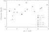 |
Fig. B.1 The typical size of the associations found in a galaxy increases as the relative spatial resolution of the detector is poorer. To use a homogeneous scale, for each galaxy-detector combination we convert the pixel scale into parsecs per pixel. Different symbols indicate different galaxies: IC 1613 (Garcia et al. 2009; Borissova et al. 2004; Ivanov 1996), NGC 6822 (Wilson 1992; Ivanov 1996), M 33 (Wilson 1991), M 31 (Magnier et al. 1993; Ivanov 1996), NGC 300 (Pietrzyński et al. 2001), NGC 7793 (Pietrzyński et al. 2005), and the sample of spiral galaxies of Bresolin et al. (1998). |
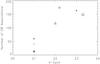 |
Fig. B.2 The number of associations found in a galaxy increases as the input catalog is deeper. Symbols as in Fig. B.1. (The sample of Bresolin et al. 1998 is not included because they provided no information about Vlimit. The sample of Ivanov 1996 is not included, as the input photometric catalogs do not cover the entire galaxies.) |
Hence, there is compelling evidence that the mean size of the associations found by friends-of-friends algorithms depends strongly on instrumental parameters, the faint limit, and the relative resolution (parsec scale) of the detector. This is not a new result, only a reflection of what already happened when working by eye on photographic plates. Automatic objective methods such as friends of friends algorithms can still play a crucial role in ensuring consistent and comparable studies of OB associations, as long as they use an equivalent instrumental set-up or take these effects into account.
Acknowledgments
This work has been partially funded by Spanish MICINN under Consolider-Ingenio 2010, programme grant CSD2006-00070 (http://www.iac.es/consolider-ingenio-gtc/), as well as grants AYA2007-67456-C02-01 and AYA2008-06166-C03-01.
References
- Allen, C. W. 2000, Allen’s Astrophyical Quatities, ed. A. N. Cox, Fourth Edition, (Springer), 388 [Google Scholar]
- Bastian, N., Ercolano, B., Gieles, M., et al. 2007, MNRAS, 379, 1302 [NASA ADS] [CrossRef] [Google Scholar]
- Battinelli, P. 1991, A&A, 244, 69 [NASA ADS] [Google Scholar]
- Bekki, K. 2008, ApJ, 680, L29 [NASA ADS] [CrossRef] [Google Scholar]
- Blaauw, A. 1964, ARA&A, 2, 213 [NASA ADS] [CrossRef] [Google Scholar]
- Borissova, J., Kurtev, R., Georgiev, L., & Rosado, M. 2004, A&A, 413, 889 [NASA ADS] [CrossRef] [EDP Sciences] [Google Scholar]
- Bresolin, F., Kennicutt, R. C., Jr., & Stetson, P. B. 1996, AJ, 112, 1009 [NASA ADS] [CrossRef] [Google Scholar]
- Bresolin, F., Kennicutt, R. C., Jr.,Ferrarese, L., et al. 1998, AJ, 116, 119 [NASA ADS] [CrossRef] [Google Scholar]
- Bresolin, F., Pietrzyński, G., Urbaneja, M. A., et al. 2006, ApJ, 648, 1007 [NASA ADS] [CrossRef] [Google Scholar]
- Bresolin, F., Urbaneja, M. A., Gieren, W., Pietrzyński, G., & Kudritzki, R.-P. 2007, ApJ, 671, 2028 [NASA ADS] [CrossRef] [Google Scholar]
- Castro, N., Herrero, A., Garcia, M., et al. 2008, A&A, 485, 41 [NASA ADS] [CrossRef] [EDP Sciences] [Google Scholar]
- Charbonnel, C., Meynet, G., Maeder, A., Schaller, G., & Schaerer, D. 1993, A&AS, 101, 415 [NASA ADS] [Google Scholar]
- Condon, J. J. 1987, ApJS, 65, 485 [NASA ADS] [CrossRef] [Google Scholar]
- Daflon, S., Cunha, K., de Araújo, F. X., Wolff, S., & Przybilla, N. 2007, AJ, 134, 1570 [NASA ADS] [CrossRef] [Google Scholar]
- Davidson, K., & Kinman, T. D. 1982, PASP, 94, 634 [NASA ADS] [CrossRef] [Google Scholar]
- Dodorico, S., & Rosa, M. 1982, A&A, 105, 410 [NASA ADS] [Google Scholar]
- Dodorico, S., & Dopita, M. 1983, Supernova Remnants and their X-ray Emission, 101, 517 [NASA ADS] [CrossRef] [Google Scholar]
- Dolphin, A. E., Saha, A., Skillman, E. D., et al. 2001, ApJ, 550, 554 [NASA ADS] [CrossRef] [Google Scholar]
- Efremov, Y. N. 2002, Astron. Rep., 46, 791 [NASA ADS] [CrossRef] [Google Scholar]
- Efremov, I. N., Ivanov, G. R., & Nikolov, N. S. 1987, Ap&SS, 135, 119 [NASA ADS] [CrossRef] [Google Scholar]
- Elmegreen, B. G., & Lada, C. J. 1977, ApJ, 214, 725 [NASA ADS] [CrossRef] [Google Scholar]
- Elmegreen, B. G., & Efremov, Y. N. 1998 [arXiv:astro-ph/9801071] [Google Scholar]
- Fabbiano, G. 1989, ARA&A, 27, 87 [NASA ADS] [CrossRef] [Google Scholar]
- Freedman, W. L. 1988a, AJ, 96, 1248 [NASA ADS] [CrossRef] [Google Scholar]
- Freedman, W. L. 1988b, ApJ, 326, 691 [NASA ADS] [CrossRef] [Google Scholar]
- Fitzgerald, M. P. 1970, A&A, 4, 234 [NASA ADS] [Google Scholar]
- Garcia, M., Herrero, A., Vicente, B., et al. 2009, A&A, 502, 1015 (Paper I) [NASA ADS] [CrossRef] [EDP Sciences] [Google Scholar]
- Garnett, D. R. 2002, ApJ, 581, 1019 [NASA ADS] [CrossRef] [MathSciNet] [Google Scholar]
- Georgiev, L., Borissova, J., Rosado, M., et al. 1999, A&AS, 134, 21 [Google Scholar]
- Georgy, C., Meynet, G., Walder, R., Folini, D., & Maeder, A. 2009, A&A, 502, 611 [NASA ADS] [CrossRef] [EDP Sciences] [Google Scholar]
- Grebel, E. K. 2001, Astrophys. Space Science Suppl., 277, 231 [Google Scholar]
- Grebel, E. K. 2002, Extragalactic Star Clusters, 207, 94 [NASA ADS] [Google Scholar]
- Herrero, A., Kudritzki, R. P., Butler, K., & Haser, S. 1992, A&A, 261, 209 [NASA ADS] [Google Scholar]
- Herrero, A., Puls, J., & Najarro, F. 2002, A&A, 396, 949 [NASA ADS] [CrossRef] [EDP Sciences] [Google Scholar]
- Herrero, A., Garcia, M., Uytterhoeven, K., et al. 2010, A&A, 513, A70 [NASA ADS] [CrossRef] [EDP Sciences] [Google Scholar]
- Hodge, P. W. 1978, ApJS, 37, 145 [NASA ADS] [CrossRef] [Google Scholar]
- Hodge, P. W. 1980, ApJ, 241, 125 [NASA ADS] [CrossRef] [Google Scholar]
- Hodge, P. 1986, Luminous Stars and Associations in Galaxies, 116, 369 [NASA ADS] [Google Scholar]
- Hodge, P., Lee, M. G., & Gurwell, M. 1990, PASP, 102, 1245 [NASA ADS] [CrossRef] [Google Scholar]
- Humphreys, R. M. 1978, ApJS, 38, 309 [NASA ADS] [CrossRef] [EDP Sciences] [Google Scholar]
- Humphreys, R. M. 1980, ApJ, 238, 65 [NASA ADS] [CrossRef] [Google Scholar]
- Ivanov, G. R. 1991, Ap&SS, 178, 227 [NASA ADS] [CrossRef] [Google Scholar]
- Ivanov, G. R. 1996, A&A, 305, 708 [NASA ADS] [Google Scholar]
- Jackson, D. C., Cannon, J. M., Skillman, E. D., et al. 2006, ApJ, 646, 192 [NASA ADS] [CrossRef] [Google Scholar]
- Kepley, A. A., Wilcots, E. M., Hunter, D. A., & Nordgren, T. 2007, AJ, 133, 2242 [NASA ADS] [CrossRef] [Google Scholar]
- Kingsburgh, R. L., & Barlow, M. J. 1995, A&A, 295, 171 [NASA ADS] [Google Scholar]
- Kroupa, P., & Weidner, C. 2005, The Initial Mass Function 50 Years Later, 327, 175 [NASA ADS] [CrossRef] [Google Scholar]
- Lee, H., Grebel, E. K., & Hodge, P. W. 2003, A&A, 401, 141 [NASA ADS] [CrossRef] [EDP Sciences] [Google Scholar]
- Lee, M. G., Freedman, W. L., & Madore, B. F. 1993, ApJ, 417, 553 [Google Scholar]
- Lejeune, T., & Schaerer, D. 2001, A&A, 366, 538 [NASA ADS] [CrossRef] [EDP Sciences] [Google Scholar]
- Loeb, A., & Barkana, R. 2001, ARA&A, 39, 19 [NASA ADS] [CrossRef] [Google Scholar]
- Lozinskaya, T. A., Moiseev, A. V., Afanas’Ev, V. L., Wilcots, E., & Goss, W. M. 2001, Astron. Rep., 45, 417 [NASA ADS] [CrossRef] [Google Scholar]
- Lozinskaya, T. A., Arkhipova, V. P., Moiseev, A. V., & Afanas’Ev, V. L. 2002, Astron. Rep., 46, 16 [NASA ADS] [CrossRef] [Google Scholar]
- Lozinskaya, T. A., Moiseev, A. V., & Podorvanyuk, N. Y. 2003, Astron. Lett., 29, 77 [NASA ADS] [CrossRef] [Google Scholar]
- Maeder, A., & Meynet, G. 2003, IAU Symp., 212, 267 [NASA ADS] [Google Scholar]
- Magrini, L., Corradi, R. L. M., Greimel, R., et al. 2005, MNRAS, 361, 517 [NASA ADS] [CrossRef] [Google Scholar]
- Magnier, E. A., Battinelli, P., Lewin, W. H. G., et al. 1993, A&A, 278, 36 [NASA ADS] [Google Scholar]
- Markova, N., & Puls, J. 2008, A&A, 478, 823 [NASA ADS] [CrossRef] [EDP Sciences] [Google Scholar]
- Martins, F., & Plez, B. 2006, A&A, 457, 637 [NASA ADS] [CrossRef] [EDP Sciences] [Google Scholar]
- Massey, P. 1998, Stellar astrophysics for the local group: VIII Canary Islands Winter School of Astrophysics, 95 [Google Scholar]
- Massey, P., Johnson, K. E., & Degioia-Eastwood, K. 1995, ApJ, 454, 151 [NASA ADS] [CrossRef] [Google Scholar]
- Massey, P., Waterhouse, E., & DeGioia-Eastwood, K. 2000, AJ, 119, 2214 [NASA ADS] [CrossRef] [Google Scholar]
- Massey, P., Zangari, A. M., Morrell, N. I., et al. 2009, ApJ, 692, 618 [NASA ADS] [CrossRef] [Google Scholar]
- Meaburn, J., Clayton, C. A., & Whitehead, M. J. 1988, MNRAS, 235, 479 [NASA ADS] [Google Scholar]
- Mokiem, M. R., de Koter, A., Vink, J. S., et al. 2007, A&A, 473, 603 [NASA ADS] [CrossRef] [EDP Sciences] [Google Scholar]
- Peimbert, M., Bohigas, J., & Torres-Peimbert, S. 1988, Rev. Mex. Astron. Astrofis., 16, 45 [NASA ADS] [Google Scholar]
- Petrovic, J., Langer, N., Yoon, S.-C., & Heger, A. 2005, A&A, 435, 247 [NASA ADS] [CrossRef] [EDP Sciences] [Google Scholar]
- Pietrzyński, G., Gieren, W., Fouqué, P., & Pont, F. 2001, A&A, 371, 497 [NASA ADS] [CrossRef] [EDP Sciences] [Google Scholar]
- Pietrzyński, G., Ulaczyk, K., Gieren, W., Bresolin, F., & Kudritzki, R. P. 2005, A&A, 440, 783 [NASA ADS] [CrossRef] [EDP Sciences] [Google Scholar]
- Puls, J. 2008, IAU Symp., 250, 25 [Google Scholar]
- Repolust, T., Puls, J., & Herrero, A. 2004, A&A, 415, 349 [NASA ADS] [CrossRef] [EDP Sciences] [Google Scholar]
- Sánchez, N., & Alfaro, E. J. 2009, ApJ, 696, 2086 [NASA ADS] [CrossRef] [Google Scholar]
- Sandage, A. 1971, ApJ, 166, 13 [NASA ADS] [CrossRef] [Google Scholar]
- Silich, S., Lozinskaya, T., Moiseev, A., et al. 2006, A&A, 448, 123 [NASA ADS] [CrossRef] [EDP Sciences] [Google Scholar]
- Skiff, B. A. 2007, VizieR Online Data Catalog, 1, 2023 [Google Scholar]
- Skillman, E. D. 2005, Rev. Mex. Astron. Astrofis., Conf. Ser., 23, 85 [Google Scholar]
- Steidel, C. C., Shapley, A. E., Pettini, M., et al. 2004, ApJ, 604, 534 [NASA ADS] [CrossRef] [Google Scholar]
- Stetson, P. B. 1987, PASP, 99, 191 [NASA ADS] [CrossRef] [Google Scholar]
- Stetson, P. B. 1994, PASP, 106, 250 [NASA ADS] [CrossRef] [Google Scholar]
- Talent, D. L. 1980, Ph.D. Thesis [Google Scholar]
- Tautvaišienė, G., Geisler, D., Wallerstein, G., et al. 2007, AJ, 134, 2318 [NASA ADS] [CrossRef] [Google Scholar]
- Tikhonov, N. A. 2005, Astron. Rep., 49, 501 [NASA ADS] [CrossRef] [Google Scholar]
- Trundle, C., Dufton, P. L., Lennon, D. J., Smartt, S. J., & Urbaneja, M. A. 2002, A&A, 395, 519 [NASA ADS] [CrossRef] [EDP Sciences] [Google Scholar]
- Trundle, C., Dufton, P. L., Hunter, I., et al. 2007, A&A, 471, 625 [NASA ADS] [CrossRef] [EDP Sciences] [Google Scholar]
- Urbaneja, M. A., Herrero, A., Kudritzki, R.-P., et al. 2005, ApJ, 635, 311 [NASA ADS] [CrossRef] [Google Scholar]
- Valdes, F. 1997, in Astronomical Data Analysis Software and Systems VI, ed. G. Hunt, & H. E. Payne (San Francisco: ASP), ASP Conf. Ser., 125, 455 [Google Scholar]
- Valdez-Gutiérrez, M., Rosado, M., Georgiev, L., Borissova, J., & Kurtev, R. 2001, A&A, 366, 35 [NASA ADS] [CrossRef] [EDP Sciences] [Google Scholar]
- Venn, K. A., Lennon, D. J., Kaufer, A., et al. 2001, ApJ, 547, 765 [NASA ADS] [CrossRef] [Google Scholar]
- Walborn, N. R. 2002, Hot Star Workshop III: The Earliest Phases of Massive Star Birth, 267, 111 [Google Scholar]
- Wilson, C. D. 1991, AJ, 101, 166 [NASA ADS] [CrossRef] [Google Scholar]
- Wilson, C. D. 1992, ApJ, 384, L29 [NASA ADS] [CrossRef] [Google Scholar]
- Wolff, S. C., Strom, S. E., Dror, D., & Venn, K. 2007, AJ, 133, 1092 [NASA ADS] [CrossRef] [Google Scholar]
- Woosley, S. E., & Bloom, J. S. 2006, ARA&A, 44, 507 [NASA ADS] [CrossRef] [Google Scholar]
All Tables
Expected Q color changes (Qneb, ∗ −Q ∗ ) due to nebular contamination as a function of spectral type.
Ages and Mup found for the associations: comparison with Georgiev et al. (1999) results.
Spectroscopic masses (Bresolin et al. 2007) vs. evolutionary masses (this work) for OB supergiants in associations.
All Figures
|
Fig. 1 Q-parameter (from our own photometry, Paper I) as a function of spectral type (from Bresolin et al. 2007). Different colors and symbols represent spectral types as indicated in the legend. Size indicates luminosity class (smallest symbols = class V, largest symbols = class I). The WO and the Be stars have been arbitrarily located in the X-axis. The Q color increases as we move towards later spectral types. Most stars with Q ≤ −0.4 are OB, Be, or WR stars. |
| In the text | |
|
Fig. 2 Location in the Q vs. Vcorr diagram of the sample stars classified by Bresolin et al. (2007). Color and symbols have the same meaning as in Fig. 1. The different groups of stars (O types, B types, Be stars, and the WO) are located in separated loci of the diagram, with a small degree of mixing. |
| In the text | |
|
Fig. 3 Effective temperature derived from isochrone analysis as a function of spectral type. Colors and symbols have the same meaning as in Fig. 1 except for the magenta symbols. The latter represent the results on SMC stars by Mokiem et al. (2007) and Massey et al. (2009), and the calibration of Trundle et al. (2007) for B stars in this galaxy (lines; thick = supergiants, thin = dwarfs), derived from quantitative spectral analysis. The WO and the Be stars have been arbitrarily located in the X-axis. Dotted lines represent the revision of spectral types by Garcia et al. (2010, in prep.). Teff derived from isochrones for our IC 1613 sample increases with earlier spectral type as expected, but flattens at O stars, hinting that color degeneracy is still a problem for these types. The Teff we derived for the IC 1613 stars roughly agrees with the trend observed in the SMC. |
| In the text | |
|
Fig. 4 Analysis of association #135, color–magnitude (top) and color–color (bottom) diagrams. Clockwise starting from top-left: a) B−V vs. V, b) Q vs. Vcorr, c) U−B vs. Q and d) B−V vs. U−B. The catalog of IC 1613 targets with good photometric quality is plotted with green dots. The likely OB stars of the association are the blue circles, and the non-OB members are represented in red. The error bars represent photometric errors. Diamonds in the Q vs. Vcorr diagram represent the OB members, their V-magnitude corrected for extinction (see Sect. 2.1). Note the larger error bars in this diagram, due to error propagation. In all panels except for the B−V vs. U−B diagram, colored lines represent the 0.2 Z⊙ isochrones of Lejeune & Schaerer (2001), whose log age is color–coded as indicated in panel a). In the B−V vs. U−B diagram, the dashed lines represent the reddening vector for O3–O9 stars. The other lines are the calibration of color with spectral type of Allen (2000) for O5-M5 main sequence stars (green), G5-M5 giants (blue), and O3-M5 supergiants (pink). |
| In the text | |
|
Fig. 5 Size distribution of the associations listed in our catalog (solid line), all having a minimum of 3 good members. The mean size is 6.1″ ± 4.5″, and the distribution peaks at 2–6″. The dotted line is the distribution of associations with 4 elements or more. The number of small associations decreases drastically, but for R > 6″ the function remains unchanged. |
| In the text | |
|
Fig. 6 Distribution of the population. To use a convenient scale, association #151 with 69 candidate OB stars was not included in this plot. Besides #151, 4 associations are well populated with more than 20 members. However, most of the groups have 10 or fewer members; a population of 3 OB stars is the most common. |
| In the text | |
|
Fig. 7 Size of the associations as a function of the number of OB stars (crosses). As expected, size increases with increasing number of members. The solid line represents the least squares fit to the points: NOB = 0.04 + 0.32 ∗ R + 0.05 ∗ R2. |
| In the text | |
|
Fig. 8 The mass of the most massive star of each association is plotted as a function of the number of bona fide OB members (black symbols). Red diamonds represent the average Mup of all associations with the same number of members, their error bars being the standard deviation. The general trend is that Mup increases with the number of members. Note however that some poorly populated associations (3-5 members) also have very high upper masses, as in the case of Orion’s Trapezium. The most populated association, #151 with 69 members, deviates from the main trend. |
| In the text | |
|
Fig. 9 The mass of the most massive star of each association is plotted as a function of stellar density, estimated as the number of bona fide OB members divided by the squared radius of the association. Different symbols represent NOB, as indicated in the legend. Associations #94 and #184 with density 1.2 and 1.9 are left out of the plot for clarity. |
| In the text | |
|
Fig. 10 Ages of OB associations in IC 1613. North is left and east is down. The association perimeters are plotted over the INT-WFC RGB image of IC 1613 (same field shown as in Fig. 9 of Paper I), with the age indicated by the contour colors. Since most associations exhibit age dispersion, the left panel shows the age of the youngest association members, and the right panel the age of the older members. Color–code is: cyan log age = 5.9, blue log age = 6.2, dark green log age = 6.5, light green log age = 6.8, yellow log age = 7.1, orange log age = 7.4, red log age = 7.7, violet log age = 8.0. The largest concentration of young associations is found in the bubble region of the galaxy in the NE lobe. |
| In the text | |
|
Fig. 11 Relative distribution of neutral hydrogen and OB associations. The grey shadow outlines the distribution of HI in IC 1613 (adapted from Fig. 1 of Silich et al. 2006). Colored contours indicate the position of the associations of Garcia et al. (2009). Color indicates the age of the youngest members, with the same color code as in Fig. 10. Numbers follow the HI fragment numbering of Silich et al. (2006). The HI cavity is surrounded by fragments 1, 10, 11, 14, and 17. |
| In the text | |
|
Fig. A.1 Color–magnitude diagrams of all groups listed in Garcia et al. (2009)’s catalog. Green dots in the background represent the complete list of targets with good photometric quality data in IC 1613. Blue circles represent the OB candidate stars of the associations, and red circles other members. Lejeune & Schaerer (2001)’s 0.2 Z⊙ isochrones are included for reference, shifted to account for distance (DM = 24.27) and foreground reddening E(B−V) = 0.02. Different colors represent different log age, as indicated in the legend. |
| In the text | |
|
Fig. A.1 continued. |
| In the text | |
|
Fig. A.1 continued. |
| In the text | |
|
Fig. A.1 continued. |
| In the text | |
|
Fig. A.1 continued. |
| In the text | |
|
Fig. A.1 continued. |
| In the text | |
|
Fig. A.1 continued. |
| In the text | |
|
Fig. A.2 Q vs. Vcorr color–magnitude diagrams of all groups listed in Garcia et al. (2009). Colored lines represent the theoretical isochrones with the same age code as in Fig. A.1, shifted by the DM, but without any correction for foreground extinction. Black diamonds represent V-magnitudes of the blue members, corrected from total extinction (foreground and local). Red circles represent the red members. These diagrams were used for age and mass determinations. |
| In the text | |
|
Fig. A.2 continued. |
| In the text | |
|
Fig. A.2 continued. |
| In the text | |
|
Fig. A.2 continued. |
| In the text | |
|
Fig. A.2 continued. |
| In the text | |
|
Fig. A.2 continued. |
| In the text | |
|
Fig. A.2 continued. |
| In the text | |
|
Fig. A.3 U−B vs. Q color–color diagrams of the associations, using the same color code as in Fig. A.1. Theoretical isochrones are included for reference. Since no extinction correction was applied, the lines mark the locus of an unreddened population. A population parallel to the isochrones but shifted indicates reddening. Note that the isochrones of all ages overlap. This provides further supporting evidence for the selection criteria (Q < −0.4) to find candidate blue massive stars used in Garcia et al. (2009). |
| In the text | |
|
Fig. A.3 continued. |
| In the text | |
|
Fig. A.3 continued. |
| In the text | |
|
Fig. A.3 continued. |
| In the text | |
|
Fig. A.3 continued. |
| In the text | |
|
Fig. A.3 continued. |
| In the text | |
|
Fig. A.3 continued. |
| In the text | |
|
Fig. A.4 B−V vs. U−B color–color diagrams. Color codes for points are the same as in Fig. A.1. The red line indicates the reddening vector for O3-O9 stars. The other lines are the calibration of color with spectral type of Allen (2000) for O5-M5 main sequence stars (green), G5-M5 giants (blue) and O3-M5 supergiants (pink). |
| In the text | |
|
Fig. A.4 continued. |
| In the text | |
|
Fig. A.4 continued. |
| In the text | |
|
Fig. A.4 continued. |
| In the text | |
|
Fig. A.4 continued. |
| In the text | |
|
Fig. A.4 continued. |
| In the text | |
|
Fig. A.4 continued. |
| In the text | |
|
Fig. B.1 The typical size of the associations found in a galaxy increases as the relative spatial resolution of the detector is poorer. To use a homogeneous scale, for each galaxy-detector combination we convert the pixel scale into parsecs per pixel. Different symbols indicate different galaxies: IC 1613 (Garcia et al. 2009; Borissova et al. 2004; Ivanov 1996), NGC 6822 (Wilson 1992; Ivanov 1996), M 33 (Wilson 1991), M 31 (Magnier et al. 1993; Ivanov 1996), NGC 300 (Pietrzyński et al. 2001), NGC 7793 (Pietrzyński et al. 2005), and the sample of spiral galaxies of Bresolin et al. (1998). |
| In the text | |
|
Fig. B.2 The number of associations found in a galaxy increases as the input catalog is deeper. Symbols as in Fig. B.1. (The sample of Bresolin et al. 1998 is not included because they provided no information about Vlimit. The sample of Ivanov 1996 is not included, as the input photometric catalogs do not cover the entire galaxies.) |
| In the text | |
Current usage metrics show cumulative count of Article Views (full-text article views including HTML views, PDF and ePub downloads, according to the available data) and Abstracts Views on Vision4Press platform.
Data correspond to usage on the plateform after 2015. The current usage metrics is available 48-96 hours after online publication and is updated daily on week days.
Initial download of the metrics may take a while.