| Issue |
A&A
Volume 708, April 2026
|
|
|---|---|---|
| Article Number | A315 | |
| Number of page(s) | 13 | |
| Section | Interstellar and circumstellar matter | |
| DOI | https://doi.org/10.1051/0004-6361/202658979 | |
| Published online | 21 April 2026 | |
PRODIGE – Envelope to disk with NOEMA
VII. (Complex) organic molecules in the NGC1333 IRAS 4B1 outflow: A new laboratory for shock chemistry
1
Max-Planck-Institut für extraterrestrische Physik,
Gießenbachstraße 1,
85748
Garching bei München,
Germany
2
Department of Physics and Astronomy, University of Rochester,
Rochester,
NY
14627,
USA
3
Max-Planck-Institut für Astronomie,
Königstuhl 17,
69117
Heidelberg,
Germany
4
Taiwan Astronomical Research Alliance (TARA),
Taiwan
5
Institute of Astronomy and Astrophysics, Academia Sinica,
PO Box 23-141,
Taipei
106,
Taiwan
6
European Southern Observatory,
Karl-Schwarzschild-Straße 2,
85748
Garching,
Germany
7
Institute de Radioastronomie Millimétrique (IRAM),
300 rue de la Piscine,
38406,
Saint-Martin d’Hères,
France
8
Zentrum für Astronomie der Universität Heidelberg, Institut für Theoretische Astrophysik,
Albert-Ueberle-Str. 2,
69120
Heidelberg,
Germany
9
Centro de Astrobiología (CAB), CSIC-INTA,
Ctra. de Ajalvir Km. 4,
28850,
Torrejón de Ardoz,
Madrid,
Spain
10
Joint ALMA Observatory,
Alonso de Córdova 3107,
Vitacura,
Santiago,
Chile
11
National Radio Astronomy Observatory,
520 Edgemont Road,
Charlottesville,
VA
22903,
USA
12
Department of Astronomy, University of Illinois,
1002 W Green St.,
Urbana,
IL
61801,
USA
13
Department of Earth, Environment and Physics, Worcester State University,
Worcester,
MA
01602,
USA
14
Observatorio Astronómico Nacional (IGN),
Alfonso XII 3,
28014
Madrid,
Spain
15
Laboratoire d’Astrophysique de Bordeaux, Université de Bordeaux,
CNRS, B18N, Allée Geoffroy Saint-Hilaire,
33615
Pessac,
France
16
Department of Earth Science Education, Seoul National University,
1 Gwanak-ro,
Gwanak-gu,
Seoul
08826,
Republic of Korea
17
SNU Astronomy Research Center, Seoul National University,
1 Gwanak-ro,
Gwanak-gu,
Seoul
08826,
Republic of Korea
★ Corresponding author: This email address is being protected from spambots. You need JavaScript enabled to view it.
Received:
15
January
2026
Accepted:
18
February
2026
Abstract
Context. Shock chemistry is an excellent tool for shedding light on the formation and destruction mechanisms of complex organic molecules (COMs). The L1157-mm outflow is the only low-mass protostellar outflow that has extensively been studied in this regard.
Aims. We mapped COM emission and derived the molecular composition of the protostellar outflow driven by the Class 0 protostar NGC 1333 IRAS 4B1 to introduce it as a new laboratory for studying the effect of shocks on COM chemistry.
Methods. We used the data taken as part of the PROtostars & DIsks: Global Evolution (PRODIGE) large program to compute integrated-intensity maps of outflow emission to identify spatial differences between species. The emission spectra were then analysed towards two positions, one in each outflow lobe, by deriving synthetic spectra and population diagrams assuming conditions of local thermodynamic equilibrium.
Results. In addition to typical outflow tracers such as SiO and CO, outflow emission is seen from H2CO, HNCO, and HC3N, as well as from the COMs CH3OH, CH3CN, and CH3CHO, and even from deuterated species such as DCN, D2CO, and CH2DOH. The maps of integrated-intensity ratios between CH3OH and DCN, D2CO, and CH3CHO reveal gradients with distance from the protostar. For DCN and D2CO, this may reflect their pre-stellar abundance profile, provided the outflow is young enough, while an explanation is still required for CH3CHO. Intensity ratio maps of HC3N and CH3CN with respect to CH3OH peak in the southern lobe where the temperatures are highest. This might indicate enhanced HC3N and CH3CN formation at this location, potentially in the warmer gas phase. Rotational temperatures are found in the range ∼50-100K, which is warmer on average than for the L1157-B1 shock spot (≲ 30K). The abundances with respect to CH3OH are higher by factors of a few than for L1157-B1.
Conclusions. For the first time, we securely detected the COMs CH3CN, CH3CHO, and CH2DOH in the IRAS 4B1 outflow, serendipitously with a limited sensitivity and bandwidth. Targeted observations will enable the discovery of new COMs and a more detailed analysis of their emission. The morphological differences between the molecules in the IRAS 4B1 outflow lobes and their relative abundances provide first proof that this outflow is a promising new laboratory for shock chemistry, which will offer crucial information on COM formation and destruction as well as on outflow structure and kinematics.
Key words: astrochemistry / stars: formation / stars: protostars / ISM: jets and outflows / ISM: molecules
© The Authors 2026
 Open Access article, published by EDP Sciences, under the terms of the Creative Commons Attribution License (https://creativecommons.org/licenses/by/4.0), which permits unrestricted use, distribution, and reproduction in any medium, provided the original work is properly cited.
This article is published in open access under the Subscribe to Open model.
Open Access funding provided by Max Planck Society.
1 Introduction
One of the key questions in astrochemistry is understanding the growth of molecular complexity during the process of star formation, including the formation and destruction processes of complex organic molecules (COMs; ≥6 atoms and carbon-bearing; Herbst & van Dishoeck 2009). In general, COMs can form either in the gas phase directly or in the solid phase on icy dust grain surfaces, from which they can desorb through numerous thermal and non-thermal processes (e.g. see the review on COM chemistry by Ceccarelli et al. 2023). To shed light on COM formation and destruction, observing sites of shock chemistry has become increasingly popular. Shock waves passing through a quiescent medium greatly affect the local chemical composition (e.g. Draine 1995). They compress and temporally heat the medium, for example, enabling endothermic reactions to take place in the gas phase and sublimating ice mantles, thereby releasing molecules into the gas phase. Stronger shocks might even sputter or completely destroy grains (e.g. Lenzuni et al. 1995; Jiménez-Serra et al. 2008; Gusdorf et al. 2008). These processes occur on a rather short timescale (hundreds to thousands of years; e.g. Burkhardt et al. 2019), adding time constraints to the molecular compositions.
Sites of shock chemistry include protostellar outflows that interact with the ambient medium. The outflow driven by the Class 0 protostar L1157-mm (L1157 hereafter) has been the target of numerous projects, in which the source presented itself as a perfect laboratory for studying COM chemistry (Bachiller & Pérez Gutiérrez 1997). Single-dish and interferometric studies that reported detections of (complex) organic molecules in this source include, for example, Arce et al. (2008, HCOOH, CH3OCHO, CH3CN), Codella et al. (2009, CH3CN), Sugimura et al. (2011, HCOOH, CH3OCHO, CH3CHO), Mendoza et al. (2014, HNCO, HCNO, NH2CHO), Fontani et al. (2014, HDCO, CH2DOH), Lefloch et al. (2017, HCOOH, H2CCO, CH3OCH3, HCOCH2OH, C2H5OH), Mendoza et al. (2018, HC3N, HC5N), and Codella et al. (2020, CH3OH, CH3CHO). Several of these studies concluded that COMs can be as abundant or even more abundant in shocked regions than in hot corinos (e.g. Arce et al. 2008; Mendoza et al. 2014; Lefloch et al. 2017) or shocked molecular clouds located in the Galactic centre (Arce et al. 2008), such as G+0.693-0.027 (e.g. see Fig. 11 in Busch et al. 2024). In addition, spatial variations in the COM emission provided insights into the likely dominating formation pathways. For example, NH2CHO emission peaks farther away from the protostar in the outflow than CH3CHO (Codella et al. 2017; López-Sepulcre et al. 2024), which has been interpreted as NH2CHO being formed later than CH3CHO. Based on astrochemical models, Codella et al. (2017) concluded that NH2CHO is dominantly formed in the post-shock gas phase, while CH3 CHO can be formed in the gas phase directly or desorbed from dust grain surfaces. With the knowledge gained from this template outflow, the search for other outflows is well underway. Complex organic molecules other than CH3OH have been mapped towards the outflow system driven by the NGC1333 IRAS 4A protobinary, which revealed emission from CH3CHO, CH3OCH3, and NH2CHO (De Simone et al. 2020), and towards the HOPS 409 outflow located in the OMC-2/3 filament (CH3CN; Bouvier et al. 2025).
We present another young protostellar outflow and discuss its potential as new laboratory for shock chemistry. The outflow driven by the Class 0 protostar NGC1333 IRAS4B1, which forms a binary system with IRAS4B2 (2450 au separation; Tobin et al. 2016), has been mapped in emission of various molecules, such as HCN (Choi 2001), H2O (Desmurs et al. 2009), H2CO (Di Francesco et al. 2001), H2S and OCS (Miranzo-Pastor et al. 2025), as well as CO, SiO, and SO (Jørgensen et al. 2007; Stephens et al. 2018; Podio et al. 2021), but COMs, other than CH3OH (Jørgensen et al. 2007; Sakai et al. 2012), remained undetected. Additionally, Herschel spectra towards the southern lobe revealed one of the richest far-infrared spectra amongst young low-mass protostellar sources, with numerous highly excited H2O, OH, CO emission lines (Herczeg et al. 2012). Following up on this, the outflow has also been observed by the James Webb Space Telescope (JWST) as part of the JWST Observations of Young protoStars (JOYS; van Dishoeck et al. 2025; Francis et al. 2025). The southern lobe was mapped in emission of H2 S(1), [Fe II] 4F7/2-4F9/2, and the CO2 15 μm band. Additional spectra show intense emission from hot C2H2 (600 K) and HCN. We report first detections of the following COMs towards the IRAS4B1 outflow: CH3CN, CH3CHO, and deuterated methanol (CH2DOH). We identify spatial variations in the molecular outflow emission and derive abundances that provide insights into the outflow structure and kinematics as well as the effect of shocks on the chemical composition.
2 Observations
2.1 PRODIGE
The IRAS 4B binary system was observed as part of the PROtostars & Disks: Global Evolution (PRODIGE; Pis: P. Caselli and Th. Henning) large program. PRODIGE is a MPG/IRAM Observatory Program (MIOP; Project ID L19MB) and targeted 30 Class 0/I protostellar systems in the Perseus molecular cloud (D = 294 ± 17 pc; Zucker et al. 2019) with the Northern Extended Millimetre Array (NOEMA) at 1 mm.
The data were taken with the Band 3 receiver and using the PolyFix correlator tuned to a local-oscillator frequency of 226.5 GHz. This setup covers a total bandwidth of 16 GHz with a channel width of 2 MHz (∼2.6 km s−1), divided into four sidebands: lower outer (214.7-218.8 GHz), lower inner (218.8222.8 GHz), upper inner (230.2-234.2 GHz), and upper outer (234.2-238.3 GHz). An additional 39 windows at high spectral resolution (62.5 kHz or ∼0.09 km s−1 channel width), each covering a 64 MHz bandwidth, were placed within the 16 GHz bandwidth. The observations probe spatial scales of approximately 300 au (corresponding to the highest angular resolution of ∼1") to 5000 au at the distance of Perseus. The phase centre is at (α,δ)J2000 = (03h29m12S.02,31°13′08″.03). The PRODIGE observations of IRAS 4B were conducted in January and April 2022 in array configurations C and D, covering baselines from 24 m to 400 m.
For the data calibration of the PRODIGE data, we used the standard observatory pipeline within the GILDAS/CLIC1 package. Continuum subtraction and data imaging were performed with the GILDAS/MAPPING package using the uv_baseline and clean tasks, respectively. For the imaging of the continuum maps, we used robust = 1 to improve the angular resolution, and for the spectral line cubes, we used natural weighting to minimise noise. More details on the data reduction and imaging can be found in Gieser et al. (2024).
Integrated-intensity maps were created using the high spectral resolution data for selected molecules except for CO and HNCO (see Sect. 3.1). Table A.1 summarises all transitions used for the various maps with their spectroscopic information. The average noise in these cubes is about 10 mJy beam−1 (62.5 kHz channel width). For the spectral line analysis, beam-averaged spectra were extracted towards two selected positions from the low spectral resolution (2 MHz) cubes, as more molecular lines are covered (see Sect. 3.3). These have noise levels of about 2 mJy beam−1.
2.2 ALPPS
Additionally, we made use of data taken with the Atacama Large Millimetre Array (ALMA) as part of the ALMA Perseus Polarization Survey (ALPPS; Cortés et al. 2025) towards IRAS4B1 at an angular resolution of 0.37" × 0.30" (PA = −20.6°). The spectral setup covers a bandwidth of 1.9 GHz from 335.5 GHz to 337.4 GHz at 0.976 MHz spectral resolution (∼0.9 kms−1). The noise level measured in the cube is 22 mJy beam−1. We used the data to produce maps of the outflow emission at high angular resolution. Additional transitions of molecules analysed with the PRODIGE data were added to the temperature and column density determinations. To combine the two datasets, we needed to smooth the ALPPS data to the angular resolution (1.1" × 0.8") and 2 MHz spectral resolution of the PRODIGE data using the convolve_to Python command and the resample command in CLASS, respectively.
3 Results
First, we study the outflow emission morphology of the detected molecules in Sect. 3.1 and highlight differences based on maps showing ratios of integrated intensities with respect to CH3OH in Sect. 3.2. The molecular rotational temperatures and column densities are derived in Sect. 3.3 towards two positions, one in each outflow lobe, and assuming local thermodynamic equilibrium (LTE). The derived molecular composition is subsequently compared to the composition in L1157-B1 in Sect. 4.
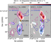 |
Fig. 1 Integrated-intensity maps towards IRAS4B1 (yellow star) for SiO 2-1 (Eu = 31 K; colour) and CH3OH 42−31 and DCN 3-2 (Eu = 45 K and 21 K, respectively; contours). The SiO maps are integrated from −25 to 6 kms−1 and 6.8 to 47 kms−1 and show emission above 10σ with σblue = 0.42 K km s−1 and σred = 0.49 K km s−1. Contours are at −30σ, −15σ, 15σ, and 30σ and then increase by a factor of 3 for CH3OH (σblue = 0.25 K kms−1 and σred = 0.23 K km s−1) and at −10σ, −5σ, 5σ, and 10σ and then increase by a factor of 3 for DCN (σblue = 0.17 K kms−1 and σred = 0.24 K km s−1). The velocity ranges (in km s−1) used for the integration of CH3OH and DCN emission are indicated in the top left corner. The half-power beam width (HPBW) is shown in the bottom left corner. Positions R1 and B1 were selected for further spectral line analysis (Sect. 3.3). The black crosses indicate H2 knots (Choi & Lee 2011). |
3.1 Emission morphology
Figure 1 shows integrated-intensity maps towards IRAS 4B1 of SiO 2-1 (colour scales), CH3OH 42−31, and DCN 3-2 (contours), separated into red- and blueshifted emission (with respect to the systemic velocity υsys = 6.8 km s−1; Busch et al. 2025). The emission extends north and south from the central protostar and can be associated with the outflow driven by that protostar. Red- and blueshifted emission at velocities of ∆υ = |υsys - υ| < 10 km s−1 is present in both lobes, suggesting that the outflow lies close to the plane of the sky. The overlap of red-and blueshifted emission is also observed for SiO (see Figs. A.1 and A.2), but in Fig. 1, we only show emission above 10σ to focus on the dominant SiO features in each lobe. Emission from CH3 OH and DCN spatially coincides with SiO for the most part. Blueshifted SiO emission close to the protostar in the southern lobe and a peak in redshifted SiO emission at ∼(0", 2.5") are not evident in CH3 OH emission, while DCN does not extend as far as SiO and CH3OH in the southern lobe. In addition, CH3OH reveals arc-like emission features that seem to start from within the main outflow lobes in the north and south and continue NW and SE, respectively. While the NW extension contains red- and blueshifted emission, the SE extension only appears in redshifted emission in our data. These features were proposed to be a second outflow by Sakai et al. (2012) based on larger-scale methanol maps, which extend beyond our field of view. The authors discussed that IRAS 4B1 might consist of two protostars, each driving an outflow. However, a second source within IRAS 4B1 remains debated. At spatial scales of ≲30 au, continuum maps at 8 mm show no clear evidence of a companion (see Fig. 34 in Segura-Cox et al. 2018), although there is extended fainter emission in addition to the peak. The emission to the east in Fig. 1 originates from the outflow driven by the companion IRAS 4B2 (see also Figs. A.2 and A.3), which we do not discuss further. Lower-excitation molecular transitions observed in the 3 mm window reveal an overall complex kinematic structure, which will be studied in detail in a forthcoming paper. These structures include, for example, the arcs identified here and a streamer candidate (Valdivia-Mena et al. 2024).
Figure A.2 shows additional channel maps of the typical outflow tracers SiO and CO, where intensities were integrated over 10 km s−1 intervals to study substructure at different velocities. At high blueshifted (−30 to −5 kms−1) and redshifted (20 to 45 km s−1 ) velocities, the emission of the IRAS 4B1 outflow is confined within the southern and northern lobes, respectively, in contrast to the broader lower-velocity emission. The reason might be that this higher-velocity component is more inclined or more collimated than the lower-velocity component. The highvelocity emission is probably associated with a jet component (see also Podio et al. 2021). The various intensity peaks or knots along both lobes might additionally indicate episodic ejection (e.g. Bachiller 1996).
Figure A.3 again shows integrated-intensity maps of blue-and redshifted emission for CH3OH and DCN and for seven additional organic (i.e. C-bearing) molecules. Example spectra towards positions R1 and B1 (see Fig. 1) are shown in Fig. A.1. Emission from H2CO and CH3OH in Fig. A.3 is most prominent in the outflow. Molecules such as CH3CHO, DCN, HC3N, CH3CN, HNCO, and D2CO show weaker emission. For HC3N and CH3CN, but maybe also for HNCO and CH3CHO, this might be an excitation effect, since the PRODIGE data only cover transitions with higher upper-level energies. Weak (signal-to-noise ratio of ∼5), compact emission from c-C3H2 is detected very close to the protostar. In addition to CH3OH, H2CO and CO also reveal arc-like emission features (Figs. A.2 and A.3). There are extended features of negative intensity, in particular, for CO and H2CO, which indicate missing flux in the PRODIGE data because of the missing short spacings (see also Gieser et al. 2025).
3.2 Spatial differences with respect to CH3OH
To determine whether there are morphological differences, we compared all molecules with CH3OH by deriving ratio maps of integrated intensity, W, that is, R = Wmo/WCH3OH, and we show them normalised by the maximum value, R/Rmax, in Fig. 2. We only plot pixels for which both integrated-intensity values are above a threshold of 5σ, where σ is the noise measured in the respective map. The integration intervals differ between molecules (same intervals as in Figs. A.1 and A.3). If we used the same (largest) interval, we would integrate over too much noise, leading to more discarded pixels for the weakest transitions. In addition, we applied a mask with a radius of 1" around the protostar because line blending is more severe in the hot corino and might bias the integrated-intensity ratios. Because upperlevel energies differ between the molecular transitions, meaning that they might probe different excitation conditions, we used two methanol transitions to reduce excitation effects: 102−93 (Eu = 165 K) with HC3N and CH3CN (Eu ≈ 130 K) and 51−42 (Eu = 56 K) with the other molecules (Eu = 20 - 65 K). Additional information on the transitions we used are summarised in Table A.1. There is a clear decrease in D2CO and DCN intensities relative to CH3OH with increasing distance from the protostar in both lobes by a factor of ∼10. In the southern lobe, a similar but less distinct gradient is seen for CH3CHO. For HC3N and CH3CN, the integrated-intensity ratio peaks in between the two H2 knots (Choi & Lee 2011) in the southern lobe. These trends might still (partially) be a consequence of different excitation conditions, but they possibly also probe different chemical processes. This is discussed further in Sect. 4.
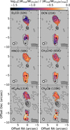 |
Fig. 2 Integrated-intensity ratios, (Wmol/WCH3OH)/(Wmol/WCH3OH)max, of various molecular transitions with either CH3OH 102,9−93,6 (Eu = 165 K; for HC3N and CH3CN) or 51,4−42,2 (Eu = 5β K; for D2CO, DCN, HNCO, and CH3CHO) towards the IRAS 4B1 outflow. Integrated intensities contain the sum of blue- and redshifted emission (see Fig. A.3 and the spectra in Fig. A.1). The ratio is only shown when both molecules are above a 5σ threshold, where σ is the noise level in the respective map. Another mask with a 1" radius around the protostar is applied to the ratios. The black contours show the integrated intensities of CH3OH, starting at −5σ, 5σ, and then increasing by a factor of 2, where σ = 0.34 K km s−1. The molecule as well as the upper-level energy of the shown transition are plotted in the top left corner. In all panels, the white star marks the position of IRAS4B1. The HPBW is shown in the bottom left corner and black crosses mark H2 knots (Choi & Lee 2011). Spectroscopic information on the shown transitions is given in Table A.1. |
3.3 Spectral-line analysis and results
For the spectral line analysis, we extracted beam-averaged spectra towards one position in the southern lobe (B1) and one in the northern lobe (R1) at (03h29m12S.09, 31°13′01″.03) and (03h29m12S.09,31°13′12″.63), respectively, which correspond to the CH3 OH emission peaks (Fig. 1). We followed the analysis strategy of Busch et al. (2025), where we already derived rotational temperatures and column densities for CH3OH and CH3CN isotopologues towards the hot corino IRAS 4B1, amongst other sources. Accordingly, we used the radiative transfer code Weeds, which is an extension of the GILDAS/CLASS software (Maret et al. 2011), and derived population diagrams (PDs; Goldsmith & Langer 1999). Both methods assume LTE. We refer to Busch et al. (2025) for details. In short: Weeds computes synthetic spectra based on five input parameters, which are column density, rotational temperature, source size, velocity offset from υsys, and line width (i.e. the full width at half maximum). We assumed that the emission is spatially resolved (i.e. a beam-filling factor of 1). The line widths and velocity offsets can be derived from fitting 1D Gaussian profiles to the spectral lines, using the CLASS command minimize, where we fitted one velocity component per molecule.
The best-fit column densities and rotational temperatures were verified with values from PDs, which are shown in Fig. A.4. The PDs were derived for CH3OH, CH3CHO, CH3CN, HC3N, CH2DOH, and D2CO, since they are the only molecules with at least three detected transitions. The temperatures and column densities that we derived with Weeds and the PDs are summarised in Table A.2 together with the other Weeds parameters. The results from Weeds and the PDs agree widely within the 1σ error bars. Some scatter between the observed data points is evident (e.g. D2CO in B1). We discussed several reasons that might lead to such scatter when we analysed the PRODIGE data in Busch et al. (2025). Weeds estimates the line optical depth based on the input parameters, yielding optically thin lines in all cases. In some PDs, when the linear fit was unreliable, we fixed the rotational temperature to obtain an estimate on the column density. The rotational temperatures range from 50 K to 100 K, without significant differences between positions B1 and R1. The column densities derived towards B1 and R1 agree within a factor of 2 and are shown in Fig. 3. They are discussed in a direct comparison with values derived towards the L1157 outflow in Sect. 4.2.
4 Discussion: A new shock-chemistry laboratory
Figure 4 summarises the main molecular features of the IRAS 4B1 outflow derived in this work, including the morphological differences of molecules with respect to CH3OH, which are further discussed in Sects. 4.1.1 and 4.1.2. In addition, we studied the morphology at higher angular resolution using ALPPS data (Sect. 4.1.3). In Sect. 4.2 we compare our results with those obtained for the L1157 outflow.
4.1 Implications from the morphology
Differences in the emission morphology between molecules can probe different physical conditions, but might also be explained by certain chemical processes. In Fig. 2, we map the outflow emission from different species in comparison with CH3OH. Figure 4 highlights the main findings. Since CH3OH is known to be formed on dust-grain surfaces and is released into the gas phase by the shocks, it is a suitable reference molecule for interpreting any morphological differences with other molecules.
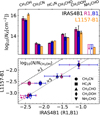 |
Fig. 3 Column densities (top) and abundances with respect to CH3OH (bottom) towards B1 and R1 in IRAS 4B1 derived in this work and values obtained for L1157-B1 (see Table A.2). The dashed and dotted black lines indicate equal abundances and a difference of a factor of 5, respectively. The empty bars or symbols with arrows indicate upper limits. |
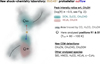 |
Fig. 4 Cartoon highlighting the main molecular features of the IRAS4B1 outflow. The main emission morphology of our reference molecule, CH3OH, is outlined in grey, including the main outflow lobes (red and blue arrows) and additional arc-like features (black lines) of currently unknown origin. The peaks of the intensity ratios with respect to CH3OH are highlighted in teal and pink, depending on the species (see Fig. 2). A spectral line analysis was performed towards positions R1 and B1 and yielded rotational temperatures of Trot = 60-100 K (Sect. 3.3). The position of the protostar is indicated in yellow. |
4.1.1 Deuterated species
The integrated-intensity ratios for the deuterated species DCN and D2CO with CH3OH (Figs. 2 and 4) significantly decrease with increasing distance from the protostar in both lobes. Recently, D2CO emission was studied towards the IRAS 4A outflows (Chahine et al. 2024), where it shows a similar trend. During the pre-stellar stage, D2 CO is more efficiently formed on dust-grain surfaces the lower the temperature, that is, closer to the centre of the pre-stellar core. Later, upon interaction with the outflow, D2CO is released from the grain surfaces. Therefore, the observed gradient along the outflow lobes might reflect the abundance profile that was built up during the pre-stellar phase, provided the molecules were recently released from grains and the gas-phase chemistry has not yet altered the abundance distribution (see also Podio et al. 2024). It is unclear whether this also applies to DCN. Based on a study of DCN towards the L1157 outflow, Busquet et al. (2017) argued that the molecule is a product of both gas- and solid-phase chemistry. Moreover, it is unclear whether DCN or HCN freeze out as efficiently during the pre-stellar phase. It was shown in pre-stellar cores that HCN remains in the gas phase, where CO is already frozen out (e.g. Hily-Blant et al. 2010; Spezzano et al. 2022). These single-dish studies probed larger spatial scales, meaning that freeze-out of DCN and HCN at smaller scales is not excluded when probed with interferometers. Predictions from astrochemical models are also inconclusive because they are heavily dependent on the underlying physical setup (priv. comm.).
4.1.2 CH3CHO, HC3N, and CH3CN
In the southern outflow lobe of IRAS 4B1, we observed decreasing CH3CHO intensity ratios relative to CH3OH (Fig. 2) with increasing distance from the protostar, while emission from both COMs is more similar in the northern lobe. In L1157-B1, CH3CHO and CH3OH coincide spatially (Codella et al. 2020), implying that CH3CHO is also formed in the solid phase or, as proposed by Codella et al. (2017, 2020), rapidly in the gas phase as soon as the reactants arrive in the gas phase from the grains. The gradient that we observe might suggest that abundances drop faster for CH3CHO than for CH3OH starting from IRAS 4B1. In contrast to CH3OH, CH3CHO can also efficiently form in hightemperature gas (e.g. Garrod et al. 2022). Therefore, to determine whether the observed emission gradient coincides with a temperature gradient, we derived maps of rotational temperature using two transitions with different upper-level energies and assuming LTE and that the transitions traced the same gas. The maps for HC3N and CH3OH are shown in Fig. 5 and reveal temperatures from 30 K to 100 K, with HC3N probing slightly higher temperatures overall. However, the general trends are similar for both molecules: in the northern lobe, the temperature increases from east to west. In the southern lobe, the temperature increases with increasing distance from the protostar, peaks in between the two H2 knots, and decreases again at the tip of the lobe. The observed emission gradient between CH3CHO and CH3OH is thus anticorrelated with the temperature gradient in the southern lobe. It is unclear what this might mean. Instead of temperature, other parameters such as density variations or cosmic rays (Pineda et al. 2024) might play a more dominating role.
The intensity ratios for HC3N and CH3CN (Figs. 2 and 4) follow the temperature map, and they do this more in the southern than in the northern lobe, suggesting that their abundances are enhanced in the higher-temperature gas. Gas-phase formation was also proposed for CH3CN and HC3N in the L1157 outflow (Codella et al. 2009; Mendoza et al. 2018). For CH3CN, this might also be supported by the fact that the column density ratio between CH3OH and CH3CN, which is ~0.005 towards the IRAS 4B1 outflow, is lower by a factor of 2 than the ratio derived towards the central hot corino (Busch et al. 2025), where even higher temperatures can facilitate gas-phase formation of CH3CN (Giani et al. 2023). In addition, JWST spectra revealed rich spectra including features from HCN and C2H2 (van Dishoeck et al. 2025) that might be involved in the enhanced production of HC3N and CH3CN (e.g. Taniguchi et al. 2019).
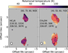 |
Fig. 5 Rotational temperatures derived from two transitions of HC3N and CH3OH assuming LTE. The rest frequencies (in GHz) and upperlevel energies of the transitions are written below the molecules. The contour levels are shown in the top right corner. The markers are the same as in Fig. 2. The HPBW is shown in the bottom left corner. |
4.1.3 Implications from ALPPS data
Observations of the L1157 outflow at high angular resolution revealed that the L1157-B1 shock spot in the blueshifted lobe consists of several smaller clumps, whose molecular compositions and physical conditions differ (Benedettini et al. 2007, 2013; Codella et al. 2009, 2020), offering insights into the outflow structure, kinematics, and chemistry. Using ALPPS data, we show integrated-intensity maps of CH3OH 71,7−61,6 (the only bright COM covered in that survey) and C34S 7-6 in Fig. A.2. Similar to L1157-B1, these observations at an about three times higher angular resolution than PRODIGE reveal a highly structured outflow morphology with several intensity peaks. In addition, the morphology of the CH3OH emission in the southern lobe resembles a bow shock, while the C34S emission forms a weak S-shape, which is indicative of jet precession (e.g. Bachiller et al. 2001). Therefore, future observations of more species at higher angular resolution will provide deeper insight into the kinematics and chemistry of the outflow.
4.2 Comparison with L1157-B1
We compare the column densities and abundances with respect to CH3 OH that we derived towards positions IRAS 4B1-B1 and R1 with literature values from L1157-B1, which were derived in interferometric observations, in Fig. 3 (see Table A.2). The column densities agree within a factor of 2 between the sources overall, while the abundances with respect to CH3OH are higher towards R1 and B1 in IRAS4B1. Most abundances differ by a factor of 5, suggesting a similar chemical composition overall. One of the reasons for the difference of a factor of 5 might be an underestimation of the optical depth of CH3OH, considering that it is quite abundant in the outflow, and hence, of its column density. The overall similar chemical composition is interesting given that both outflows have different physical conditions. We derived the molecular composition at positions that are much closer to IRAS 4B1 (D ~ 1500-2000 au) than L1157-B1 is to its protostar (D ~ 30 000 au; Arce et al. 2008). Related to this, the rotational temperatures that we derived, for example, for CH3OH and CH3CHO (60-80 K), are significantly higher than towards L1157-B1, but also higher than towards the IRAS4A outflows (~10-20 K; De Simone et al. 2020; Codella et al. 2020). On the other hand, the rotational temperatures derived from CH3 CN in L1157-B1 range from 50K to 130K (Codella et al. 2009), similar to what we derived for this molecule. Generally, higher temperatures suggest that volume densities are higher, which might indicate stronger shocks (McKee & Hollenbach 1980). Moreover, the observed sub-thermal excitation of H2O at 1500 K observed in Herschel spectra in the southern lobe requires a density of about 106 cm−3 (Herczeg et al. 2012), which makes the IRAS 4B1 outflow a site of a high (pre-)shock density (see also van Dishoeck et al. 2025).
The different maximum spatial extent also implies different outflow ages or shock timescales. The compact IRAS4B1 outflow was proposed to be very young (a few hundred years; Choi 2001 ; Yildiz et al. 2015), and is therefore younger than the L1157 outflow (a few thousand years; e.g. Yildiz et al. 2015; Kwon et al. 2015; Podio et al. 2016). The timescale associated with the age of the IRAS 4B1 outflow might be crucial for post-shock gas-phase chemistry. For example, a period of ≲1000 yr is associated with the delayed formation of NH2CHO compared with CH3CHO in L1157-B1, which was mentioned in the introduction (Sect. 1; Codella et al. 2017). We did not detect NH2CHO. If it were to remain undetected in more sensitive future observations towards the outflow of IRAS 4B1, the chemistry in the post-shock gas might be in an early phase, meaning that a significant amount of NH2CHO has not yet formed. Therefore, the young age of the IRAS 4B1 outflow might be the perfect testbed for studying the grain-surface versus gas-phase formation of COMs.
5 Summary
We used data taken as part of the PRODIGE large program and ALPPS to study the emission of organic molecules, including COMs, towards the outflow driven by the Class 0 protostar NGC1333 IRAS 4B1. We posit that this outflow has the potential to be a new laboratory for the study of COMs in shocked media. Our main findings are listed below:
We reported the first detection of the COMs CH3CN, CH3CHO, and deuterated methanol (CH2DOH) towards this outflow.
We investigated the morphology of the outflow emission of these three COMs, CH3OH, and simpler species (HC3N, HNCO, CO, DCN, D2CO, H2CO, and c-C3H2); The deuterated species DCN and D2CO showed a gradient with respect to CH3OH, where they would peak closer to the protostar. This likely reflects the DCN and D2CO abundance profiles from the pre-stellar phase. Acetaldehyde (CH3CHO) showed a similar gradient in the southern lobe, which still needs an explanation. In the southern lobe, the intensity ratios of HC3N and CH3CN with respect to CH3OH followed the temperature variations, suggesting that the N-bearing molecules are (additionally) formed in the hotter post-shock gas phase.
The methanol emission at high angular resolution using ALPPS data revealed a highly structured outflow morphology, which is also seen in L1157-B1.
Towards one position in the northern lobe (R1) and one position in the southern lobe (B1), we derived higher rotational temperatures (50-100 K) and higher abundances on average with respect to CH3OH by factors of a few than towards L1157-B1.
Future observations at higher angular resolution that are as sensitive as those towards L1157-B1 will enable us to detect less abundant COMs and build a comprehensive chemical inventory of the IRAS4B1 outflow, which we can compare to the inventory of the central hot corino. Together with modelling efforts, this will deliver crucial information on COM formation and destruction processes as well as outflow structure and kinematics.
Acknowledgements
The authors thank the IRAM staff at the NOEMA observatory for their support in the observations and data calibration. This work is based on observations carried out under project number L19MB with the IRAM NOEMA Interferometer. IRAM is supported by INSU/CNRS (France), MPG (Germany) and IGN (Spain). L.A.B., J.E.P., P.C., M.J.M., C.G., Y.L., D.S., Y.C., L.M., S.N. acknowledge the support by the Max Planck Society. D.S. was funded by the Deutsche Forschungsgemeinschaft (DFG, German Research Foundation) - project number: 550639632. This project is co-funded by the European Union (ERC, SUL4LIFE, grant agreement No101096293). A.F. also thanks project PID2022-137980NB-I00 funded by the Spanish Ministry of Science and Innovation/State Agency ofResearch MCIN/AEI/10.13039/501100011033 and by “ERDF A way of making Europe”.
References
- Arce, H. G., Santiago-García, J., Jørgensen, J. K., Tafalla, M., & Bachiller, R. 2008, ApJ, 681, L21 [NASA ADS] [CrossRef] [Google Scholar]
- Bachiller, R. 1996, ARA&A, 34, 111 [Google Scholar]
- Bachiller, R., & Pérez Gutiérrez, M. 1997, ApJ, 487, L93 [Google Scholar]
- Bachiller, R., Pérez Gutiérrez, M., Kumar, M. S. N., & Tafalla, M. 2001, A&A, 372, 899 [NASA ADS] [CrossRef] [EDP Sciences] [Google Scholar]
- Balança, C., Dayou, F., Faure, A., Wiesenfeld, L., & Feautrier, N. 2018, MNRAS, 479, 2692 [Google Scholar]
- Baskakov, O. I., Alekseev, E. A., Dyubko, S. F., & Shevyrev, A. S. 1988, Opt. Spectrosc., 64, 130 [Google Scholar]
- Ben Khalifa, M., Dagdigian, P. J., & Loreau, J. 2023, MNRAS, 523, 2577 [NASA ADS] [CrossRef] [Google Scholar]
- Benedettini, M., Viti, S., Codella, C., et al. 2007, MNRAS, 381, 1127 [Google Scholar]
- Benedettini, M., Viti, S., Codella, C., et al. 2013, MNRAS, 436, 179 [Google Scholar]
- Blanco, S., López, J. C., Lesarri, A., & Alonso, J. L. 2006, J. Am. Chem. Soc., 128, 12111 [Google Scholar]
- Bocquet, R., Demaison, J., Cosléou, J., et al. 1999, J. Mol. Spectrosc., 195, 345 [NASA ADS] [CrossRef] [Google Scholar]
- Bouvier, M., Giani, L., Chahine, L., et al. 2025, MNRAS, 539, 2380 [Google Scholar]
- Burkhardt, A. M., Shingledecker, C. N., Le Gal, R., et al. 2019, ApJ, 881, 32 [Google Scholar]
- Busch, L. A., Belloche, A., Garrod, R. T., Müller, H. S. P., & Menten, K. M. 2024, A&A, 681, A104 [NASA ADS] [CrossRef] [EDP Sciences] [Google Scholar]
- Busch, L. A., Pineda, J. E., Sipilä, O., et al. 2025, A&A, 699, A359 [NASA ADS] [CrossRef] [EDP Sciences] [Google Scholar]
- Busquet, G., Fontani, F., Viti, S., et al. 2017, A&A, 604, A20 [CrossRef] [EDP Sciences] [Google Scholar]
- Ceccarelli, C., Codella, C., Balucani, N., et al. 2023, in Astronomical Society of the Pacific Conference Series, 534, Protostars and Planets VII, eds. S. Inutsuka, Y. Aikawa, T. Muto, K. Tomida, & M. Tamura, 379 [Google Scholar]
- Chahine, L., Ceccarelli, C., De Simone, M., et al. 2024, MNRAS, 534, L48 [Google Scholar]
- Chandra, S., & Kegel, W. H. 2000, A&AS, 142, 113 [Google Scholar]
- Chardon, J., Genty, C., Guichon, D., Sungur, N., & Theobald, J. 1974, Rev. Phys. Appl. (Paris), 9, 961 [Google Scholar]
- Chen, W., Bocquet, R., Wlodarczak, G., & Boucher, D. 1991, Int. J. Infrared Millimeter Waves, 12, 987 [NASA ADS] [CrossRef] [Google Scholar]
- Choi, M. 2001, ApJ, 553, 219 [NASA ADS] [CrossRef] [Google Scholar]
- Choi, M., & Lee, J.-E. 2011, J. Korean Astron. Soc., 44, 201 [Google Scholar]
- Codella, C., Benedettini, M., Beltrán, M. T., et al. 2009, A&A, 507, L25 [NASA ADS] [CrossRef] [EDP Sciences] [Google Scholar]
- Codella, C., Ceccarelli, C., Caselli, P., et al. 2017, A&A, 605, L3 [NASA ADS] [CrossRef] [EDP Sciences] [Google Scholar]
- Codella, C., Ceccarelli, C., Bianchi, E., et al. 2020, A&A, 635, A17 [NASA ADS] [CrossRef] [EDP Sciences] [Google Scholar]
- Cortés, P. C., Pineda, J. E., Hsieh, T.-H., et al. 2025, ApJ, 992, L31 [Google Scholar]
- Dangoisse, D., Willemot, E., & Bellet, J. 1978, J. Mol. Spectrosc., 71, 414 [NASA ADS] [CrossRef] [Google Scholar]
- De Simone, M., Codella, C., Ceccarelli, C., et al. 2020, A&A, 640, A75 [NASA ADS] [CrossRef] [EDP Sciences] [Google Scholar]
- de Zafra, R. L. 1971, ApJ, 170, 165 [NASA ADS] [CrossRef] [Google Scholar]
- DeLeon, R. L., & Muenter, J. S. 1985, J. Chem. Phys., 82, 1702 [NASA ADS] [CrossRef] [Google Scholar]
- Denis-Alpizar, O., Stoecklin, T., Guilloteau, S., & Dutrey, A. 2018, MNRAS, 478, 1811 [Google Scholar]
- Desmurs, J. F., Codella, C., Santiago-García, J., Tafalla, M., & Bachiller, R. 2009, A&A, 498, 753 [NASA ADS] [CrossRef] [EDP Sciences] [Google Scholar]
- Di Francesco, J., Myers, P. C., Wilner, D. J., Ohashi, N., & Mardones, D. 2001, ApJ, 562, 770 [NASA ADS] [CrossRef] [Google Scholar]
- Draine, B. T. 1995, Ap&SS, 233, 111 [NASA ADS] [CrossRef] [Google Scholar]
- Dumouchel, F., Faure, A., & Lique, F. 2010, MNRAS, 406, 2488 [NASA ADS] [CrossRef] [Google Scholar]
- Endres, C. P., Schlemmer, S., Schilke, P., Stutzki, J., & Müller, H. S. P. 2016, J. Mol. Spectrosc., 327, 95 [NASA ADS] [CrossRef] [Google Scholar]
- Faure, A., Lique, F., & Wiesenfeld, L. 2016, MNRAS, 460, 2103 [NASA ADS] [CrossRef] [Google Scholar]
- Fontani, F., Codella, C., Ceccarelli, C., et al. 2014, ApJ, 788, L43 [Google Scholar]
- Francis, L., van Dishoeck, E. F., Caratti o Garatti, A., et al. 2025, A&A, 694, A174 [NASA ADS] [CrossRef] [EDP Sciences] [Google Scholar]
- Gadhi, J., Lahrouni, A., Legrand, J., & Demaison, J. 1995, J. Chim. Phys., 92, 1984 [Google Scholar]
- Gardner, F. F., Godfrey, P. D., & Williams, D. R. 1980, MNRAS, 193, 713 [Google Scholar]
- Garrod, R. T., Jin, M., Matis, K. A., et al. 2022, ApJS, 259, 1 [NASA ADS] [CrossRef] [Google Scholar]
- Giani, L., Ceccarelli, C., Mancini, L., et al. 2023, MNRAS, 526, 4535 [NASA ADS] [CrossRef] [Google Scholar]
- Gieser, C., Pineda, J. E., Segura-Cox, D. M., et al. 2024, A&A, 692, A55 [NASA ADS] [CrossRef] [EDP Sciences] [Google Scholar]
- Gieser, C., Caselli, P., Segura-Cox, D. M., et al. 2025, A&A, 701, A165 [NASA ADS] [CrossRef] [EDP Sciences] [Google Scholar]
- Goldsmith, P. F., & Langer, W. D. 1999, ApJ, 517, 209 [Google Scholar]
- Gusdorf, A., Cabrit, S., Flower, D. R., & Pineau Des Forêts, G. 2008, A&A, 482, 809 [NASA ADS] [CrossRef] [EDP Sciences] [Google Scholar]
- Herbst, E., & van Dishoeck, E. F. 2009, ARA&A, 47, 427 [Google Scholar]
- Herczeg, G. J., Karska, A., Bruderer, S., et al. 2012, A&A, 540, A84 [NASA ADS] [CrossRef] [EDP Sciences] [Google Scholar]
- Hily-Blant, P., Walmsley, M., Pineau Des Forêts, G., & Flower, D. 2010, A&A, 513, A41 [NASA ADS] [CrossRef] [EDP Sciences] [Google Scholar]
- Hirota, E., Sugisaki, R., Nielsen, C. J., & Sørensen, G. O. 1974, J. Mol. Spectrosc., 49, 251 [NASA ADS] [CrossRef] [Google Scholar]
- Jiménez-Serra, I., Caselli, P., Martín-Pintado, J., & Hartquist, T. W. 2008, A&A, 482, 549 [NASA ADS] [CrossRef] [EDP Sciences] [Google Scholar]
- Jørgensen, J. K., Bourke, T. L., Myers, P. C., et al. 2007, ApJ, 659, 479 [Google Scholar]
- Kryvda, A. V., Gerasimov, V. G., Dyubko, S. F., Alekseev, E. A., & Motiyenko, R. A. 2009, J. Mol. Spectrosc., 254, 28 [NASA ADS] [CrossRef] [Google Scholar]
- Kukolich, S. G., & Nelson, A. C. 1971, Chem. Phys. Lett., 11, 383 [NASA ADS] [CrossRef] [Google Scholar]
- Kurland, R. J., & Bright Wilson, Jr., E. 1957, J. Chem. Phys., 27, 585 [Google Scholar]
- Kwon, W., Fernández-López, M., Stephens, I. W., & Looney, L. W. 2015, ApJ, 814, 43 [NASA ADS] [CrossRef] [Google Scholar]
- Lefloch, B., Ceccarelli, C., Codella, C., et al. 2017, MNRAS, 469, L73 [Google Scholar]
- Lenzuni, P., Gail, H.-P., & Henning, T. 1995, ApJ, 447, 848 [NASA ADS] [CrossRef] [Google Scholar]
- López-Sepulcre, A., Codella, C., Ceccarelli, C., Podio, L., & Robuschi, J. 2024, A&A, 692, A120 [NASA ADS] [CrossRef] [EDP Sciences] [Google Scholar]
- Mallinson, P. D., & de Zafra, R. L. 1978, Mol. Phys., 36, 827 [NASA ADS] [CrossRef] [Google Scholar]
- Maret, S., Hily-Blant, P., Pety, J., Bardeau, S., & Reynier, E. 2011, A&A, 526, A47 [NASA ADS] [CrossRef] [EDP Sciences] [Google Scholar]
- McKee, C. F., & Hollenbach, D. J. 1980, ARA&A, 18, 219 [Google Scholar]
- Mendoza, E., Lefloch, B., López-Sepulcre, A., et al. 2014, MNRAS, 445, 151 [NASA ADS] [CrossRef] [Google Scholar]
- Mendoza, E., Lefloch, B., Ceccarelli, C., et al. 2018, MNRAS, 475, 5501 [NASA ADS] [CrossRef] [Google Scholar]
- Miranzo-Pastor, J. J., Fuente, A., Navarro-Almaida, D., et al. 2025, A&A, 700, A251 [NASA ADS] [CrossRef] [EDP Sciences] [Google Scholar]
- Moskienko, E. M., & Dyubko, S. F. 1991, Radiophys. Quant. Electron., 34, 181 [NASA ADS] [CrossRef] [Google Scholar]
- Motiyenko, R. A., & Margulès, L. 2025, A&A, 699, A348 [NASA ADS] [CrossRef] [EDP Sciences] [Google Scholar]
- Müller, H. S. P., Brown, L. R., Drouin, B. J., et al. 2015, J. Mol. Spectrosc., 312, 22 [CrossRef] [Google Scholar]
- Pearson, J. C., Müller, H. S. P., Pickett, H. M., Cohen, E. A., & Drouin, B. J. 2010, J. Quant. Spec. Radiat. Transf., 111, 1614 [NASA ADS] [CrossRef] [Google Scholar]
- Pearson, J. C., Yu, S., & Drouin, B. J. 2012, J. Mol. Spectrosc., 280, 119 [NASA ADS] [CrossRef] [Google Scholar]
- Pineda, J. E., Sipilä, O., Segura-Cox, D. M., et al. 2024, A&A, 686, A162 [NASA ADS] [CrossRef] [EDP Sciences] [Google Scholar]
- Podio, L., Codella, C., Gueth, F., et al. 2016, A&A, 593, L4 [NASA ADS] [CrossRef] [EDP Sciences] [Google Scholar]
- Podio, L., Tabone, B., Codella, C., et al. 2021, A&A, 648, A45 [NASA ADS] [CrossRef] [EDP Sciences] [Google Scholar]
- Podio, L., Ceccarelli, C., Codella, C., et al. 2024, A&A, 688, L22 [NASA ADS] [CrossRef] [EDP Sciences] [Google Scholar]
- Rabli, D., & Flower, D. R. 2010, MNRAS, 406, 95 [Google Scholar]
- Sahnoun, E., Wiesenfeld, L., Hammami, K., & Jaidane, N. 2018, J. Phys. Chem. A, 122, 3004 [NASA ADS] [CrossRef] [Google Scholar]
- Sakai, N., Ceccarelli, C., Bottinelli, S., Sakai, T., & Yamamoto, S. 2012, ApJ, 754, 70 [NASA ADS] [CrossRef] [Google Scholar]
- Schöier, F. L., van der Tak, F. F. S., van Dishoeck, E. F., & Black, J. H. 2005, A&A, 432, 369 [Google Scholar]
- Segura-Cox, D. M., Looney, L. W., Tobin, J. J., et al. 2018, ApJ, 866, 161 [Google Scholar]
- Smirnov, I. A., Alekseev, E. A., Ilyushin, V. V., et al. 2014, J. Mol. Spectrosc., 295, 44 [NASA ADS] [CrossRef] [Google Scholar]
- Spezzano, S., Caselli, P., Sipilä, O., & Bizzocchi, L. 2022, A&A, 664, L2 [NASA ADS] [CrossRef] [EDP Sciences] [Google Scholar]
- Stephens, I. W., Dunham, M. M., Myers, P. C., et al. 2018, ApJS, 237, 22 [NASA ADS] [CrossRef] [Google Scholar]
- Sugimura, M., Yamaguchi, T., Sakai, T., et al. 2011, PASJ, 63, 459 [NASA ADS] [Google Scholar]
- Taniguchi, K., Herbst, E., Caselli, P., et al. 2019, ApJ, 881, 57 [Google Scholar]
- Thorwirth, S., Müller, H. S. P., & Winnewisser, G. 2000, J. Mol. Spectrosc., 204, 133 [NASA ADS] [CrossRef] [Google Scholar]
- Tobin, J. J., Looney, L. W., Li, Z.-Y., et al. 2016, ApJ, 818, 73 [CrossRef] [Google Scholar]
- Tucker, K. D., & Tomasevich, G. R. 1973, J. Mol. Spectrosc., 48, 475 [Google Scholar]
- Valdivia-Mena, M. T., Pineda, J. E., Caselli, P., et al. 2024, A&A, 687, A71 [NASA ADS] [CrossRef] [EDP Sciences] [Google Scholar]
- van Dishoeck, E. F., Tychoniec, E., Rocha, W. R. M., et al. 2025, A&A, 699, A361 [NASA ADS] [CrossRef] [EDP Sciences] [Google Scholar]
- Vorob’eva, E. M., & Dyubko, S. F. 1994, Radiophys. Quant. Electron., 37, 155 [Google Scholar]
- Wiesenfeld, L., & Faure, A. 2013, MNRAS, 432, 2573 [NASA ADS] [CrossRef] [Google Scholar]
- Xu, L.-H., Fisher, J., Lees, R. M., et al. 2008, J. Mol. Spectrosc., 251, 305 [NASA ADS] [CrossRef] [Google Scholar]
- Yamada, K. M. T., Moravec, A., & Winnewisser, G. 1995, Z. Naturforschung A, 50, 1179 [Google Scholar]
- Yang, B., Stancil, P. C., Balakrishnan, N., & Forrey, R. C. 2010, ApJ, 718, 1062 [Google Scholar]
- Yildiz, U., Goldsmith, P., Pineda, J., & Langer, W. 2015, in American Astronomical Society Meeting Abstracts, 225, 451.09 [Google Scholar]
- Zucker, C., Speagle, J. S., Schlafly, E. F., et al. 2019, ApJ, 879, 125 [NASA ADS] [CrossRef] [Google Scholar]
Appendix A Additional tables and figures
Figure A.1 shows example spectra towards positions R1 and B1 (Fig. 1) for selected molecules. Vertical lines indicate the integration limits used for Figs. 1, 2, and A.3. Figure A.2 shows channel maps towards the IRAS4B Class 0 binary of SiO and CO using PRODIGE data and CH3OH and C34S using ALPPS data. Intensities were integrated from −33 to 47 km s−1 in 10 km s−1 intervals for SiO and CO and from 3 to 11 km s−1 in 2 km s−1 intervals for CH3OH and C34S. The ALPPS data at about three times higher angular resolution reveal the highly structured outflow morphology. Figure A.3 shows integrated intensity maps of red- and blueshifted emission from various organic molecules using the PRODIGE data. The derived population diagrams (PDs) are shown in Fig. A.4.
Table A.1 summarises spectroscopic properties of molecular transitions used for the various maps in this work. Table A.2 shows the results of the LTE spectral-line analyses towards positions IRAS4B1-B1 and IRAS4B1-R1 in the outflow, using the radiative transfer code Weeds (Maret et al. 2011) and PDs (Goldsmith & Langer 1999). Column densities derived towards the L1157-B1 outflow shock spot are provided as well. Table A.3 provides references for the spectroscopic information for the analysed molecules.
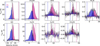 |
Fig. A.1 Average spectra of selected molecules extracted from a 1" aperture towards positions R1 and B1 (see Fig. 1). The dashed black line indicates the systemic velocity of 6.8 km s−1, while the red and blue dashed lines indicate the outer integration limits for the respective molecule used in Figs. 1, 2, and A.3. Despite the narrow band not covering all the H2CO emission, we used it for the H2CO map as it shows more structure. |
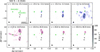 |
Fig. A.2 Integrated-intensity maps for SiO and CO (PRODIGE) towards IRAS 4B1 and IRAS 4B2 (green stars) and for CH3OH and C34S (ALPPS, next page) zoomed in (cf. the dashed black rectangle in the CO panels) on IRAS4B1. The intensities were integrated over intervals of 10 kms−1 (SiO and CO) and 2 kms−1 (CH3OH and C34S). Contour levels are at −10σ, 10σ and then increase by a factor of 2, where σ = 0.24K kms−1 (SiO), 0.27K kms−1 (CO), and 0.34K kms−1 (CH3OH and C34S). The black crosses mark H2 knots (Choi & Lee 2011). The HPBWs are shown in the bottom left corners. |
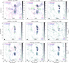 |
Fig. A.3 Integrated-intensity maps towards IRAS 4B1 and 4B2 (green stars) for various molecules. The transitions we used and their upper-level energies are given above the respective panel. Contours are at −5σ, 5σ, and 10σ, and then increase by a factor of 3 for all but SiO, CO, H2CO, and CH3OH, for which contours start at −10σ and 10σ. The noise level, σ, is measured in the respective map and is written in the bottom right corner. The velocity range (in kms−1) used for the integration is indicated in the top left corner. The grey scale shows the sum of the red- and blueshifted maps. The HPBW is shown in the bottom left corner. The dashed grey circle indicates the primary beam (~23″). The positions R1 and B1 (green circles) are selected for further spectral line analysis. |
Molecular transitions used in this work for integrated-intensity and temperature maps.
Weeds parameters and results of the population diagram analysis.
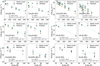 |
Fig. A.4 Population diagrams towards positions R1 and B1 (see Fig. A.3). The results of the linear fit to the observed data points (teal circles) are shown in the respective panel. The observed data were corrected for contaminating emission and both observed and modelled data (orange squares) are corrected for optical depth (for details see Busch et al. 2025). |
All Tables
Molecular transitions used in this work for integrated-intensity and temperature maps.
All Figures
|
Fig. 1 Integrated-intensity maps towards IRAS4B1 (yellow star) for SiO 2-1 (Eu = 31 K; colour) and CH3OH 42−31 and DCN 3-2 (Eu = 45 K and 21 K, respectively; contours). The SiO maps are integrated from −25 to 6 kms−1 and 6.8 to 47 kms−1 and show emission above 10σ with σblue = 0.42 K km s−1 and σred = 0.49 K km s−1. Contours are at −30σ, −15σ, 15σ, and 30σ and then increase by a factor of 3 for CH3OH (σblue = 0.25 K kms−1 and σred = 0.23 K km s−1) and at −10σ, −5σ, 5σ, and 10σ and then increase by a factor of 3 for DCN (σblue = 0.17 K kms−1 and σred = 0.24 K km s−1). The velocity ranges (in km s−1) used for the integration of CH3OH and DCN emission are indicated in the top left corner. The half-power beam width (HPBW) is shown in the bottom left corner. Positions R1 and B1 were selected for further spectral line analysis (Sect. 3.3). The black crosses indicate H2 knots (Choi & Lee 2011). |
| In the text | |
|
Fig. 2 Integrated-intensity ratios, (Wmol/WCH3OH)/(Wmol/WCH3OH)max, of various molecular transitions with either CH3OH 102,9−93,6 (Eu = 165 K; for HC3N and CH3CN) or 51,4−42,2 (Eu = 5β K; for D2CO, DCN, HNCO, and CH3CHO) towards the IRAS 4B1 outflow. Integrated intensities contain the sum of blue- and redshifted emission (see Fig. A.3 and the spectra in Fig. A.1). The ratio is only shown when both molecules are above a 5σ threshold, where σ is the noise level in the respective map. Another mask with a 1" radius around the protostar is applied to the ratios. The black contours show the integrated intensities of CH3OH, starting at −5σ, 5σ, and then increasing by a factor of 2, where σ = 0.34 K km s−1. The molecule as well as the upper-level energy of the shown transition are plotted in the top left corner. In all panels, the white star marks the position of IRAS4B1. The HPBW is shown in the bottom left corner and black crosses mark H2 knots (Choi & Lee 2011). Spectroscopic information on the shown transitions is given in Table A.1. |
| In the text | |
|
Fig. 3 Column densities (top) and abundances with respect to CH3OH (bottom) towards B1 and R1 in IRAS 4B1 derived in this work and values obtained for L1157-B1 (see Table A.2). The dashed and dotted black lines indicate equal abundances and a difference of a factor of 5, respectively. The empty bars or symbols with arrows indicate upper limits. |
| In the text | |
|
Fig. 4 Cartoon highlighting the main molecular features of the IRAS4B1 outflow. The main emission morphology of our reference molecule, CH3OH, is outlined in grey, including the main outflow lobes (red and blue arrows) and additional arc-like features (black lines) of currently unknown origin. The peaks of the intensity ratios with respect to CH3OH are highlighted in teal and pink, depending on the species (see Fig. 2). A spectral line analysis was performed towards positions R1 and B1 and yielded rotational temperatures of Trot = 60-100 K (Sect. 3.3). The position of the protostar is indicated in yellow. |
| In the text | |
|
Fig. 5 Rotational temperatures derived from two transitions of HC3N and CH3OH assuming LTE. The rest frequencies (in GHz) and upperlevel energies of the transitions are written below the molecules. The contour levels are shown in the top right corner. The markers are the same as in Fig. 2. The HPBW is shown in the bottom left corner. |
| In the text | |
|
Fig. A.1 Average spectra of selected molecules extracted from a 1" aperture towards positions R1 and B1 (see Fig. 1). The dashed black line indicates the systemic velocity of 6.8 km s−1, while the red and blue dashed lines indicate the outer integration limits for the respective molecule used in Figs. 1, 2, and A.3. Despite the narrow band not covering all the H2CO emission, we used it for the H2CO map as it shows more structure. |
| In the text | |
|
Fig. A.2 Integrated-intensity maps for SiO and CO (PRODIGE) towards IRAS 4B1 and IRAS 4B2 (green stars) and for CH3OH and C34S (ALPPS, next page) zoomed in (cf. the dashed black rectangle in the CO panels) on IRAS4B1. The intensities were integrated over intervals of 10 kms−1 (SiO and CO) and 2 kms−1 (CH3OH and C34S). Contour levels are at −10σ, 10σ and then increase by a factor of 2, where σ = 0.24K kms−1 (SiO), 0.27K kms−1 (CO), and 0.34K kms−1 (CH3OH and C34S). The black crosses mark H2 knots (Choi & Lee 2011). The HPBWs are shown in the bottom left corners. |
| In the text | |
|
Fig. A.3 Integrated-intensity maps towards IRAS 4B1 and 4B2 (green stars) for various molecules. The transitions we used and their upper-level energies are given above the respective panel. Contours are at −5σ, 5σ, and 10σ, and then increase by a factor of 3 for all but SiO, CO, H2CO, and CH3OH, for which contours start at −10σ and 10σ. The noise level, σ, is measured in the respective map and is written in the bottom right corner. The velocity range (in kms−1) used for the integration is indicated in the top left corner. The grey scale shows the sum of the red- and blueshifted maps. The HPBW is shown in the bottom left corner. The dashed grey circle indicates the primary beam (~23″). The positions R1 and B1 (green circles) are selected for further spectral line analysis. |
| In the text | |
|
Fig. A.4 Population diagrams towards positions R1 and B1 (see Fig. A.3). The results of the linear fit to the observed data points (teal circles) are shown in the respective panel. The observed data were corrected for contaminating emission and both observed and modelled data (orange squares) are corrected for optical depth (for details see Busch et al. 2025). |
| In the text | |
Current usage metrics show cumulative count of Article Views (full-text article views including HTML views, PDF and ePub downloads, according to the available data) and Abstracts Views on Vision4Press platform.
Data correspond to usage on the plateform after 2015. The current usage metrics is available 48-96 hours after online publication and is updated daily on week days.
Initial download of the metrics may take a while.