| Issue |
A&A
Volume 709, May 2026
|
|
|---|---|---|
| Article Number | A173 | |
| Number of page(s) | 15 | |
| Section | Interstellar and circumstellar matter | |
| DOI | https://doi.org/10.1051/0004-6361/202558787 | |
| Published online | 22 May 2026 | |
ALMAGAL
VIII. Early phases of triggered star formation in source AG286.0716–1.8229
1
INAF-Istituto di Astrofisica e Planetologia Spaziale,
Via Fosso del Cavaliere 100,
00133
Roma,
Italy
2
I. Physikalisches Institut, Universität zu Köln,
Zülpicher Str. 77,
50937
Köln,
Germany
3
Max-Planck-Institut für Radioastronomie,
Auf dem Hügel 69,
53121
Bonn,
Germany
4
INAF-Osservatorio Astrofisico di Arcetri,
Largo E. Fermi 5,
50125
Firenze,
Italy
5
Max-Planck-Institute for Extraterrestrial Physics (MPE),
Garching bei München,
Germany
6
Laboratory for the study of the Universe and eXtreme phenomena (LUX), Observatoire de Paris,
Meudon,
France
7
Dipartimento di Fisica, Università di Roma Tor Vergata,
Via della Ricerca Scientifica 1,
00133
Roma,
Italy
8
Institut de Ciències de l’Espai (ICE), CSIC, Campus UAB, Carrer de Can Magrans s/n,
08193,
Bellaterra (Barcelona),
Spain
9
Institut d’Estudis Espacials de Catalunya (IEEC),
08860,
Castelldefels (Barcelona),
Spain
10
University of Connecticut, Department of Physics,
2152 Hillside Road, Unit 3046 Storrs,
CT
06269,
USA
11
Institute of Astronomy and Astrophysics, Academia Sinica,
11F of ASMAB, AS/NTU No. 1, Sec. 4, Roosevelt Road,
Taipei
10617,
Taiwan
12
East Asian Observatory,
660 N. A’ohoku, Hilo,
Hawaii,
HI
96720,
USA
13
Max Planck Institute for Astronomy,
Königstuhl 17,
69117
Heidelberg,
Germany
14
Jodrell Bank Centre for Astrophysics,
Oxford Road, The University of Manchester,
Manchester
M13 9PL,
UK
15
Universität Heidelberg, Zentrum für Astronomie, Institut für Theoretische Astrophysik,
Heidelberg,
Germany
16
Universität Heidelberg, Interdisziplinäres Zentrum für Wissenschaftliches Rechnen,
Heidelberg,
Germany
17
Center for Astrophysics | Harvard & Smithsonian,
60 Garden St,
Cambridge,
MA
02138,
USA
18
Elizabeth S. and Richard M. Cashin Fellow at the Radcliffe Institute for Advanced Studies at Harvard University,
10 Garden Street,
Cambridge,
MA
02138,
USA
19
Center for Data and Simulation Science, University of Cologne,
Germany
20
ASTRON, Netherlands Institute for Radio Astronomy,
Oude Hoogeveensedijk 4,
Dwingeloo,
7991
PD,
The Netherlands
21
Dipartimento di Fisica e Astronomia, Università degli Studi di Firenze,
Via G. Sansone 1,
50019
Sesto Fiorentino, Firenze,
Italy
22
SKA Observatory, Jodrell Bank, Lower Withington,
Macclesfield,
SK11 9FT,
UK
23
UK ALMA Regional Centre Node
M13 9PL,
UK
24
Universidad Nacional Autònoma de Mèxico, Instituto de Radioastronomìa y Astrofísica,
Apartado Postal 3-72,
58089
Morelia Michoacàn,
Mexico
25
Departamento de Astronomía, Universidad de Chile,
Casilla 36-D,
Santiago,
Chile
26
National Radio Astronomy Observatory,
520 Edgemont Road,
Charlottesville,
VA
22903,
USA
27
Université Paris-Saclay, Université Paris-Cité, CEA, CNRS, AIM,
91191
Gif-sur-Yvette,
France
28
School of Engineering and Physical Sciences, Isaac Newton Building, University of Lincoln, Brayford Pool,
Lincoln
LN6 7TS,
UK
29
Korea Astronomy and Space Science Institute,
776 Daedeokdae-ro, Yuseong-gu,
Daejeon
34055,
Republic of Korea
30
University of Science and Technology, Korea (UST),
217 Gajeongro, Yuseong-gu,
Daejeon
34113,
Republic of Korea
31
UK Astronomy Technology Centre, Royal Observatory Edinburgh,
Blackford Hill,
Edinburgh
EH9 3HJ,
UK
32
Faculty of Physics, University of Duisburg-Essen,
Lotharstraße 1,
47057
Duisburg,
Germany
33
Jet Propulsion Laboratory, California Institute of Technology,
4800 Oak Grove Drive,
Pasadena,
CA
91109,
USA
34
INAF-Istituto di Radioastronomia & Italian ALMA Regional Centre,
Via P. Gobetti 101,
40129
Bologna,
Italy
35
Department of Astronomy, School of Science, The University of Tokyo,
7-3-1 Hongo, Bunkyo,
Tokyo
113-0033,
Japan
36
Department of Astrophysics, University of Vienna,
Turkenschanzstrasse 17,
1180
Vienna,
Austria
37
Dipartimento di Fisica e Astronomia, Alma Mater Studiorum – Università di Bologna,
Italy
38
SRON Netherlands Institute for Space Research,
Landleven 12,
9747
AD
Groningen,
The Netherlands
39
Kapteyn Astronomical Institute, University of Groningen,
The Netherlands
40
Zhejiang Laboratory,
Hangzhou
311100,
PR
China
41
Universidad Autonoma de Chile,
Pedro de Valdivia 425,
9120000
Santiago de Chile,
Chile
★ Corresponding author: This email address is being protected from spambots. You need JavaScript enabled to view it.
Received:
24
December
2025
Accepted:
20
March
2026
Abstract
Context. Several theoretical and observational studies have shown that new waves of triggered star formation can be induced by the feedback from newly formed massive protostars, due to the expansion of H II regions.
Aims. We used the millimeter dust continuum data of the ALMAGAL survey and the Anderson et al. (2014) catalog of H II regions to search for signatures of possible triggered star formation at its onset, and selected one ALMAGAL source for ALMA follow-up observations.
Methods. For this study we selected the source AG286.0716–1.8229, in which six cores were detected at a resolution of ~7600 au, but only two at a higher resolution. The four cores not detected at higher resolution are prestellar core candidates. We used archival data from the SARAO Meerkat Galactic Plane Survey and Rapid Askap Continuum Survey to confirm whether a H II region is present in the field. We observed the source with ALMA in Band 4, covering the emission of DCO+(2–1), N2D+(2–1), DCN (2–1), and CH3CCH (9–8), to infer from the chemical composition and temperature estimates whether these cores are in an early phase of the star-formation process, which allows us to classify them as prestellar cores. The new Band 4 continuum image revealed additional three cores outside of the ALMAGAL field of view (FoV), making a total of nine cores in the region, eight of which are located along an arch that has a radius of ~0.75 pc. We also used the continuum and molecular emission to estimate the mass of these cores, to determine whether they are gravitationally bound or transient objects.
Results. We have derived a spectral index between −0.14 and −0.4, in the frequency range of 0.8–1.6 GHz for the candidateH II region, which is consistent with optically thin free-free emission. The H II region spatially coincides (as projected on the plane of the sky) with the position of one of the cores, which in the new ALMA Band 4 observations does not have a compact morphology. The N2D+and DCO+emission peaks at the position of three out of four prestellar core candidates, and the overall emission in both the line and the continuum, which extends outside of the FoV of the ALMAGAL observations, reveals a clear arched shape centered on the H II region. We were able to estimate the gas temperature of only the most evolved core, using the CH3CCH emission. The resulting value of 39 ± 5 K is also an upper limit for the other cores. Using plausible temperature ranges for each core, based on the information from chemical tracers and the dust continuum, we derived mass ranges for the cores (~2–16 M⊙) as well as ranges for the virial parameter (~0.3–5). All the cores along the arch have virial parameters consistent with bound objects, with only one exception.
Conclusions. Comparing the typical separation and mass of the cores with those expected in the case of the collect and collapse scenario and with the thermal Jean length and mass, the best agreement is found with the characteristic scales in the case of triggered star formation. The same methodology can be applied to further ALMAGAL sources to identify optimal targets to study a larger sample of prestellar cores in an environment affected by the presence of a H II region.
Key words: astrochemistry / stars: formation / HII regions / ISM: molecules
© The Authors 2026
 Open Access article, published by EDP Sciences, under the terms of the Creative Commons Attribution License (https://creativecommons.org/licenses/by/4.0), which permits unrestricted use, distribution, and reproduction in any medium, provided the original work is properly cited.
This article is published in open access under the Subscribe to Open model. This email address is being protected from spambots. You need JavaScript enabled to view it. to support open access publication.
1 Introduction
The formation of OB stars has a deep impact on the environment in which they are born, since they ionize their surrounding medium and create H II regions. The expansion of these H II regions could trigger a new wave of star formation. During the expansion of the ionizing front, previously diffuse homogeneous material can be collected and compressed. It then collapses due to gravity (Elmegreen & Lada 1977, collect and collapse scenario). Alternatively, the expanding H II regions can compress preexisting inhomogeneous materials containing dense structures, making them reach the condition for their collapse (Bertoldi 1989), or a combination of the two effects could be at work (Walch et al. 2015).
The triggering effect of H II regions for new star formation has been predicted by numerical simulations (e.g. Hosokawa & Inutsuka 2005; Dale et al. 2007) and confirmed in various observational cases (e.g. Zavagno et al. 2006, 2007, 2010; Deharveng et al. 2008; Fontani et al. 2012; Liu et al. 2015; Palmeirim et al. 2017; Zhou et al. 2020; Sharma et al. 2022). However, the majority of the observational studies have analyzed evolved H II regions and looked at the distribution of already formed young stellar objects (YSOs) or the CO emission (Elia et al. 2007; Thompson et al. 2012; Kendrew et al. 2012), while only a few cases have analyzed young star-forming material using higher density tracers (e.g. Fontani et al. 2012; Tackenberg et al. 2013; Kendrew et al. 2016; Palmeirim et al. 2017; Zhang et al. 2024; Kim et al. 2025). The details of this triggered star formation, and the possible differences between star formation triggered by the presence of H II regions and the scenario without feedback from already formed massive stellar objects, have not been fully explored, especially at the onset of the process. Our goal is to investigate the early stage of the process in the two scenarios.
For this reason, we used the ALMA evolutionary study of high-mass protocluster formation in the GALaxy (ALMAGAL) survey (Molinari et al. 2025) to search for sites of the early phase of triggered star formation. ALMAGAL observed more than 1000 high-mass clumps in different environments in our Galaxy, and at different evolutionary stages, with the Atacama Large Millimeter/Submillimeter Array (ALMA) in Band 6, down to a resolution of ~1000 au (Sánchez-Monge et al. 2025; Coletta et al. 2025). To search for cores in the earliest evolutionary stage, we compared the continuum emission of the ALMAGAL field at the full resolution of ~1000 au1 and at an intermediate resolution of ~5000 au2 (see Section 2.1 and Sánchez-Monge et al. 2025 for more details). Comparing the two sets of images, it is possible that a compact source in the maps at ~5000 au is not identified above the noise limits in the ~1000 au if the radial profile of the source is flat, as in the case of prestellar cores (e.g. Caselli et al. 2019a). In such a case, the same flux will be spread over a larger number of smaller beams in the full-resolution image, and can be undetected. This will not happen for more evolved cores that will have a peaked radial profile structure. Therefore, to search for candidate prestellar cores we looked for compact sources detected at ~5000 au, but not matched with any core at ~1000 au, which we refer to hereafter as disappearing cores. Moreover, to have good candidates for this pilot study, we searched for H II regions or candidate H II regions in the ALMAGAL fields in the catalog of Anderson et al. (2014) closer than 1 pc to one or more disappearing cores. These disappearing cores are candidate prestellar cores in regions influenced by the presence of a possible H II region.
Among the ~1000 regions in ALMAGAL, we identified AG286.0716–1.8229 as a very promising region in which to study the presence of very early-stage dense cores in the vicinity of an expanding H II region, which has four disappearing cores, as is shown in detail in Section 3. The aim of this study is to confirm the nature of the disappearing cores as bound objects in a pristine phase of the star-formation process, and investigate the scenario of triggered star formation in the source using new observations in ALMA Band 4 of deuterated molecular species and continuum archival data at the centimeter wavelength. In fact, in the early stages of star formation in regions with a temperature below 20 K and density above ~105 cm−3, the deuteration process takes place (e.g. Caselli & Ceccarelli 2012; Fontani et al. 2011, 2014). This process leads to a significant enhancement of the abundance of several deuterated species. Some of the species affected are DCO+and N2D+, which are included in our observations. Once this scenario is tested, the method could be expanded to other regions to improve the statistics on these objects and have a base to evaluate systemic differences between the star formation process in the presence of H II regions and non-triggered star formation, from the time of their onset.
In Section 2, we present the dataset of the observations. In Section 3 we analyze the continuum emission in different bands and the line emission from new ALMA Band 4 observations. In Section 4, we discuss the results. In Section 5 we discuss whether the formation of the cores analyzed is really triggered by the presence of an H II region. In Section 6, we summarize our main results.
2 Observations
Table 1 gives a small summary of the dataset analyzed in Section 3 and described more in details in the following subsections.
2.1 ALMA Band 4 observations
Our new observations were carried out with ALMA on 16 August 2024 in configuration C-4 (Project 2023.1.01386.S, PI: C. Mininni). The source AG286.0716–1.8229 has coordinates l = 286.0716° and b = −1.8229°, and a heliocentric distance of 8.5 kpc (Molinari et al. 2025). The source was observed with an elevation of between ~45° and ~53° for a total of ~3.2 hrs on source. The sources selected for the phase and water vapor radiometer calibrations were J1032–5917 and J1019–6047.
The continuum and cubes analyzed in this paper are the products of the standard pipeline and imaging (version 2023.1.0.124, Hunter et al. 2023) provided by ALMA using CASA version 6.5.4.9 (CASA Team 2022) using a robust value of 0.5. The linear resolution of the observations is of 0.83″ × 0.59″ (~6000 au) and the maximum recoverable scale is 7.5″ (~0.3 pc), while the field of view (FoV) is of 58.4″. We observed the source AG286.0716–1.8229 in four spectral windows in Band 4, centered around the emission lines of DCO+(2–1) (144.077 GHz), N2D+(2–1) (154.217 GHz), DCN (2–1) (144.828 GHz), and CH3CCH 9–8 (K = 0: 153.817 GHz). Each spectral window has a bandwidth of 117.19 MHz and a spectral resolution of 0.098 MHz (~0.2 km s−1).
2.2 ALMA Band 6 observations
The observations in ALMA Band 6 are part of the ALMAGAL large program (project code: 2019.1.00195.L in Cycle 7; PI: Molinari, Schilke, Battersby, Ho; Molinari et al. 2025; Sánchez-Monge et al. 2025) that was observed between October 2019 and July 2022. The target name in the ALMA archive (internal ID) for source AG286.0716–1.8229 is 646390. To achieve the requested linear resolution without losing information on diffuse material at the clump scale, each target was observed with the 7-m array (hereafter 7M) and with two configurations of the main ALMA array. AG286.0716–1.8229 was observed in configurations C-3 (TM2) and C-6 (TM1). The ALMAGAL team developed a dedicated pipeline to obtain the final cubes, using joint deconvolution of the various configurations observed, and that includes self-calibration for the most intense sources. A detailed description of the data reduction, together with a quality assessment of the final products, is presented in Sánchez-Monge et al. (2025). The ALMAGAL pipeline produced continuum maps and cubes obtained by the joint deconvolution of 7M and TM2 data only (hereafter 7M+TM2), which reach a linear resolution of ~7600 au (~0.89″), and of all the available configurations (hereafter 7M+TM2+TM1) that reach the maximum resolution of ~1400 au (~0.17″) for source AG286.0716–1.8229. The resolution reached for the images and cubes of AG286.0716–1.8229 is worse than the typical average resolution in the ALMAGAL sample (~5000 au and ~1000 au), since this is one of the farthest sources in the sample at 8.5 kpc heliocentric distance. The diameter of the FoV of the observations is 35.4″ (down to the 30% primary beam response).
The spectral setup of the observations covers four spectral windows in total: two spectral windows with a 1.9 GHz bandwidth and a spectral resolution of 0.98 MHz (~1.3 km s−1) centered at 217.8 GHz and 220.0 GHz, and two higher-resolution spectral windows with a 0.47 GHz bandwidth and spectral resolution of 0.24 MHz (~0.3 km s−1) centered at 218.3 GHz and 220.6 GHz, respectively. The spectral frequency ranges observed include the frequency of emission of SiO (5–4) transition, with a rest frequency of 217.105 GHz.
2.3 Archival data
We collected the continuum emission of AG286.0716–1.8229 in the infrared and at centimeter wavelength from surveys in the literature. We obtained the emission at 3.6 and 4.5 μm from the Deep GLIMPSE survey observed by Spitzer Infrared Array Camera (IRAC) (Whitney et al. 2011) with ~2″ resolution. No data for the coordinates of source AG286.0716–1.8229 were available at 5.8 and 8.0 μm from the NASA/IPAC Infrared Science Archive (IRSA). We recovered the emission at 23 cm for this source from both the SARAO MeerKAT Galactic Plane Survey (SMGPS; Goedhart et al. 2024)3 with an angular resolution of 8″ and the Rapid ASKAP Continuum Survey (RACS; McConnell et al. 2020; Hale et al. 2021; Duchesne et al. 2024, 2025) with an angular resolution of 24″ at 0.88 GHz and ~10″ at 1.35 and 1.65 GHz.
3 Analysis
3.1 Millimeter continuum emission
In Figure 1, we show 150 GHz continuum emission from the ALMA Band 4 data (left) and the 219 GHz continuum emission from the ALMAGAL 7M+TM2 and 7M+TM2+TM1 data (center and right, respectively). Coletta et al. (2025) and Coletta et al. in prep. used the algorithm CuTEx (Molinari et al. 2011, 2017) to identify the compact sources inside the ALMAGAL continuum 7M+TM2 and 7M+TM2+TM1 images. CuTEx identifies compact sources as maxima of curvature in maps by analyzing their second derivatives. This method allows for an easier identification of compact sources, which stand out in the curvature images, while diffuse and background emission is strongly dampened. Once the peaks in the curvature maps were identified, they were fit (in the original map) with 2D elliptical Gaussians plus a background that can be of a first- or second-order polynomial4, in order to obtain the positions and sizes of the sources (semimajor axis, θA, semiminor axis, θB, and position angle, PA) and the integrated flux (background-subtracted). We used the identification numbers defined by CuTEx on the ALMAGAL continuum 7M+TM2, already shown in Fig. 1, to identify the various sources throughout this work. CuTEx identified six sources at ~7600 au resolution, but only four at ~1400 au resolution (Coletta et al. 2025), three of which are subfragments of the source #4 in the 7600 au data. Therefore, there are four compact sources identified in the 7600 au resolution image that have no counterparts in the 1400 au resolution image in the 219 GHz continuum data. These are core #1, #2, #5, and #6. These sources are prestellar core candidates, without a centrally peaked structure yet, as is discussed in Sect. 4.1. This is supported by the fact that the integrated fluxes of cores #2,#5, and #6 are larger than or comparable to the integrated flux density of core #3 (see Table 2).
The 150 GHz continuum data (left panel) shows an emission overall similar to that of the 219 GHz 7M+TM2 data. However, the emission of core #1 is not as bright as the rest of the cores and it is not compact, while from the CuTEx algorithm extraction we performed on this continuum image the compact core #5 is resolved into two cores, due to the better angular resolution. Moreover, this new dataset has a larger FoV than the ALMAGAL data, which reveals the presence of further emission. Considering this newly observed area, it is evident that the compact cores are located in an arch-shaped region centered close to the position of core #1. The radius of this arch is ~18.0″, which corresponds to ~0.75 pc at the distance of AG286.0716–1.8229. There are three new cores identified along the arch outside the ALMAGAL FoV, which are labeled as core #7, #8, and #9, respectively (see Fig. 1). In Table 2 we report the coordinates, the integrated flux densities of the cores, and their mean radius, r, as derived from CuTEx (r = d tan θ, where ![Mathematical equation: $\[\theta=\sqrt{\theta_{A} \theta_{B}}\]$](/articles/aa/full_html/2026/05/aa58787-25/aa58787-25-eq1.png) and d = 8.5 kpc is the source distance) of cores from #2 to #9.
and d = 8.5 kpc is the source distance) of cores from #2 to #9.
In the last column of Table 2 we report the average column density of each core. All the cores show similar values; therefore, the “disappearing” nature of some of them is not related to their average density. Moreover, this ensures that the molecular emission that we discuss in Sect. 3.3 is not biased (e.g., the density of the core is not above the critical density of the line observed) by the different density in different cores.
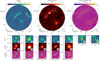 |
Fig. 1 Top left panel: continuum emission at 150 GHz; the magenta circle represents the FoV of the ALMAGAL observations, while the dashed white circle visually represent the arch-shaped region where the continuum cores are detected. Top middle panel: ALMAGAL 7M+TM2 continuum emission; the cyan boxes are the footprint of the zoom-ins in the lower panels. Top right panel: ALMAGAL 7M+TM2+TM1 continuum emission. The dashed white circle in all the three top panels visually represents the 0.75 pc radius circle along which all cores, except core #1, are aligned. Lower panel: zoom-ins of the regions delimited in cyan in the top middle panel, where we kept the same color scale for the three different datasets. The cyan ellipses represent the compact sources identified with CuTEx in the ALMAGAL 7M+TM2 data, with their identification number reported in cyan, while the black ellipses and the green ellipses are the compact sources identified with CuTEx in the ALMA Band 4 data and the ALMAGAL 7M+TM2+TM1 data, respectively. |
Properties of the continuum cores along the arch-shaped structure.
3.2 Centimeter continuum emission
In Fig. 2, we show the continuum emission of this region at 23 cm from SMGPS, with the contours of continuum emission Article number, page 4 of 15 from ALMA observations at 150 GHz superimposed. The center of the arched emission is consistent with the position of bright radio emission. The position of the peak of the 23 cm emission matches within 3″ with the position of a candidate H II region from the catalog of Anderson et al. (2014), which used the morphology seen in the emission in WISE bands to identify H II regions, together with radio emission and line emission. The source was classified as a “candidate” due to a lack of data from radio recombination lines (RRLs) to confirm the presence of ionized material.
We collected all the available archival data in the literature to build the most complete radio spectral energy distribution (SED) of this source, encompassing core #1 identified in the continuum images of ALMA Band 4 and 6. Using the data cube with the emission in different sub-bands for SMGPS, and the emission at the three wavelengths of RACS, we were able to construct the SED between 0.88 GHz and 1.65 GHz. The source is point-like, as a preliminary 2D Gaussian fit performed using the Cube Analysis and Rendering Tool for Astronomy (CARTA, Wang et al. 2020) matches the angular resolution of the data. We then performed aperture photometry using a circular aperture of 2 times the resolution of the data (~20″). The SED in the available range shows a flat profile (see Fig. 3). The spectral index, α (assuming Sν ∝ να), from the fit of the data is −0.4 ± 0.4, mostly driven by the point at 1.65 GHz from SMGPS, while the flux density from RACS data at the same frequency is consistent with a −0.1 ± 0.4 spectral index. The spectral index values and their error were derived with a Monte Carlo Markov chain linear fit to the points between 0.8 GHz and 1.6 GHz, using 100 walkers and 500 steps. Both values of α are consistent with optically thin free-free emission, as is seen from α values derived in the same range from known H II regions using SMGPS from Goedhart et al. (2024). We also included in the SED the flux densities inside the region of emission at 23 cm in the two ALMA Bands that are dominated by the dust emission, which correspond to what we previously defined as core #1. We calculated the spectral index between the point at 150 GHz and at 220 GHz, first removing the contribution from free-free emission extrapolated from the two possible fits of the first part of the SED. The range of the spectral index is then between 2.7 (assuming α = −0.43 for the free-free emission) and 4.2 (assuming α = −0.14 for the free-free emission), which corresponds to the emission of dust along the same line of sight as the emission of the H II region. The value of the exponent of the power-law of dust emissivity β (with β = α − 2 in the Rayleigh-Jeans regime) for this source is in the range of 0.7–2.2. These values are consistent with typical values found in the interstellar medium (Planck Collaboration XI 2014). The commonly used value of β~1.7–2 corresponds to a grain distribution with sizes of between 100 Å and 0.3 μm (Weingartner & Draine 2001), while larger grains result in lower values of β, reaching values below 1 for grain sizes above 1 mm (Cacciapuoti et al. 2023, and references therein). However, given the more diffuse morphology of core #1 from its 150 GHz emission, we do not consider it to be a compact core and we exclude it from further analysis to determine whether this is a prestellar core.
The number of Lyman continuum photons emitted by the ionizing source and that generate the H II region can be calculated using the radio flux density, following the relation given by Matsakis et al. (1976):
![Mathematical equation: $\[N_{\mathrm{Ly}}=7.5 \times 10^{46}\left(\frac{S_\nu}{\mathrm{Jy}}\right)\left(\frac{D}{\mathrm{kpc}}\right)^2\left(\frac{\nu}{\mathrm{GHz}}\right)^{0.1}\left(\frac{T_e}{10^4 \mathrm{~K}}\right)^{-0.45} \text { phot.} \mathrm{s}^{-1},\]$](/articles/aa/full_html/2026/05/aa58787-25/aa58787-25-eq2.png) (1)
(1)
where Sν is the flux density of the source at frequency ν, D is the distance of the source, and Te is the electron temperature. Balser et al. (2011) provided a relation between Te and the galactocentric distance of a source that estimated at the galactocentric distance of AG286.0716-1.8229(~10 kpc) gives a value of Te ~ 9000 K. Given the presence of some scatter in the relation, we considered a range of Te = 8000–10 000 K. Considering the flux density from the average continuum map of SMGPS to be 10.5 mJy at 1.36 GHz, and using the source distance of 8.5 kpc, the rate of ionizing photon is in the range of 5.9–6.5 × 1046 photons s−1, corresponding to a star of spectral type B0.5 (Panagia 1973).
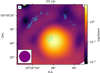 |
Fig. 2 Radio emission at 23 cm from the SMGPS in color scale (units millijansky/beam), with overimposed cyan contours (4,10, and 20 times the rms) of the ALMA Band 4 continuum emission at 150 GHz. The beam of the 23 cm emission is shown in purple in the bottom left corner. The beam of the ALMA 150 GHz emission is shown in cyan in the upper left corner. |
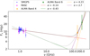 |
Fig. 3 Spectral energy distribution of the radio emission between 0.88 GHz and 219 GHz from SMGPS, RACS, ALMAGAL, and the new data presented in this paper. The dashed green line is the best linear fit between 0.88 and 1.65 GHz including all the data points; the dashed red line is the best linear fit between 0.88 and 1.65 GHz if the SMGPS point at 1.65 GHz is removed; the dashed purple line is the best fit of the 150 and 219 GHz flux, after removing the free-free contamination assuming the green fit; and the dashed yellow line is the same as the purple one, but calculating the free-free contamination using the dashed red line. |
3.3 Molecular emission
Figure 4 shows the integrated intensity (moment-0) maps of DCO+ (2–1) (upper left), N2D+ (2–1) (upper center), and DCN (2–1) (upper right) emission. The moments were created using a velocity range defined pixel by pixel. We created the mask used for the moments integration following these steps: (1) we calculated the root mean squared (σ) of the cube for each pixel, using the first 500 channels of the cubes, which were determined to be free of any emission; (2) we created a first mask of the cube to include the voxels of emission above 5σ; (3) we created a second mask to include the voxels of two consecutive channels with emission above 2σ; (4) we eliminated from the mask in step 3 all the voxels that do not include a previous voxel above 5σ, i.e., defined in the mask in point 2; and (5) we enlarged the mask obtained from point 4 of 0.25×FWHM of the beam in the spatial directions and of two channels at the beginning and at the end of the range of integration in the spectral direction, to include possible faint emission at the tail of the line profile. The mask obtained in step 5 is the final mask that we used to create the moments. As a last step, from the σ and the number of channels of integration of each pixel, we constructed a map of the moment-0 rms, and blanked from the moment maps the pixels where the moment-0 signal-to-noise ratio (S/N) was below 3.
Moreover, we extracted averaged spectra toward the cores (see Fig. A.1) and we report the detection at S/N>5 of the transitions observed in ALMA Band 4 in Table 3. From Fig. 4, the emission of DCO+ (top row of the lower panel) is bright and compact toward the disappearing cores #2, #5, and #6, while even if it is still present it does not peak or shows enhancement toward cores #3, #4, #7, #8, and #9. An enhancement and peak morphology is seen for N2D+ (middle row of the lower panel) toward cores #2, #5, and #6; in the remaining cores, it is detected from the spectra and moment-0 maps only toward cores #7 and #8, but without a peaked morphology. Conversely, the emission of DCN (bottom row of the lower panel) shows a bright peaked emission toward the position of core #4. However, DCN is detected toward the majority of other cores. Its morphology always shows a peak inside the area of the cores, often offset from the center of the cores, or with two peaks.
As for the continuum, the molecular emission in ALMA Band 4 revealed the presence of material outside the continuum cores with other spots in which the emission is enhanced in those molecular species both outside and inside the ALMAGAL FoV. Those could also be the positions of further prestellar cores, better revealed by the molecular emission, as seen in two star-forming regions with H2D+ by Redaelli et al. 2021. Table 3 gives a summary of where the different molecular species shows a peaked emission.
We also report in Fig. 5 the velocity of the gas along the line of sight and the full-width at half maximum (FWHM) of the line using DCO+(2–1), which shows the most widespread emission in the region. In the moment-1 map we identify a velocity gradient in the radial direction centered on the H II region position, a signature of an expanding shell. Similar gradients have been found in other shells around ultracompact H II (UC H II) regions and H II regions (e.g. Fontani et al. 2012; Wang et al. 2016). Cores are located at the position where the velocities match the median of the velocity gradient, with the exception of core #1. The FWHM of the DCO+ (2–1) is narrow, with values of between 0.6 and 1.5 km s−1 in the largest part of the region, with the exception of core #4, where it reaches values of up to ~2 km s−1.
To further investigate the presence of an expanding shell or collision between the medium outside the shell and the ionizing front that potentially triggered new star formation, we report in Fig. 6 the position-velocity (PV) plots of the DCO+(2–1) emission along cuts at the positions of the cores in the radial direction, i.e., in the direction that connects each core with the center of the H II region. For cores #4, #7, #8, and #9 there is not bright enough emission coincident with the center of the cut, i.e., the peak position of the core, as has already been seen in the moment-0 map. For the other cores, we observe a radial velocity gradient, which in the case of cores #5 and #6 has a breaking point at their position. As was stated above, the radial velocity gradient is likely the signature of an expanding shell, while the breaks in the gradient in the p–v plot resemble those shown in Fig. 5 of Arce et al. (2011) at the interface between the expanding bubble and the material surrounding it.
The CH3CCH (9–8) emission has only been detected toward core #4, with the transitions K = 0, and 1 clearly detected above 5 sigma, and two other transitions marginally detected. We extracted an average spectrum toward this core, and used the Spectral Line Identification and Modelling (SLIM) tool of the MAdrid Data CUBe Analysis package (MADCUBA Martín et al. 2019) to perform a line fitting. To analyze CH3CCH we selected the Cologne Database for Molecular Spectroscopy catalog (CDMS; Endres et al. 2016)5, and used SLIM to generate synthetic spectra under the assumption of local thermodynamic equilibrium (LTE). SLIM allows one to fit the spectrum using nonlinear least-squares LTE fit to the data using the Levenberg–Marquardt algorithm, comparing the modeled spectra with the observed one. The free parameters fit by the LTE model are the molecular column density (N), excitation temperature (Tex), central velocity of the line emission, and FWHM of the Gaussian line profiles. The resulting best fit to the spectrum is shown in Fig. 7). The derived temperature is Tex = 39 ± 5 K, while the column density of this species is N = (2.1 ± 0.2) × 1014 cm−2.
Lastly, to investigate the possible presence of outflows, we created the moment-0 and moment-1 maps of SiO (5–4) transition, using the 7M+TM2 cubes of the ALMAGAL project. These are shown in Appendix in Fig. C.1. Among the cores inside the ALMAGAL FoV, only the core #4 is associated with SiO emission, which shows a velocity gradient in the northeast-southwest direction.
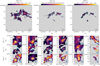 |
Fig. 4 Top panel: moment-0 map of DCO+(2–1) (left), N2D+(2–1) (middle), and DCN (2–1) (right). Bottom panels: zooms-in of the three moment-0 maps in the boxes delimited in cyan in the upper panels. The cyan and white ellipses identify the compact cores extracted with CuTEx from the ALMAGAL 7M+TM2 continuum and ALMA Band 4 continuum, respectively. Some of the zoom-in boxes have the intensity multiplied by a factor reported in red in the top right corner of the box, to highlight the emission with respect to the color scale adopted for the full maps. |
Molecular emission from the continuum cores along the arch-shaped structure.
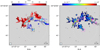 |
Fig. 5 Moment-1 (left) of DCO+(2–1) and FWHM (right) from the fit pixel by pixel of the line profile of DCO+(2–1). The color scales unit is km s−1. The dashed line boxes are the same as in Fig. 1. The cyan ellipses are the compact cores detected. The dashed white circle is the 0.75 pc radius circle along which the cores are aligned. |
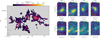 |
Fig. 6 Left panel: moment-0 maps of DCO+(2–1) with shown in white the cuts for the PV plots, centered at the peak positions of the cores. Right panels: PV plots for each core in the arch. The vertical white line delimits the position of the peak of the core. The dashed magenta line delimits the contours where the emission is half and two thirds of the maximum. |
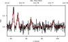 |
Fig. 7 Average spectrum of CH3CCH (9–8) over core #4 in black. In red we show the simulated spectrum obtained using the best-fit parameters with MADCUBA. |
4 Discussion
4.1 Radial profile of continuum emission
We used the continuum emission in ALMA Band 6 7M+TM2 data to construct the radial profile of emission of the cores from #1 to #6, and then compare the profiles of disappearing and not-disappearing ones. For every core from #1 to #6, we cut a region around the core in which by visual evaluation the emission is not affected by the presence of nearby cores. Each core was identified as an ellipse with a specific center position (x0, y0), PA, semimajor to semiminor axis ratio (θA/θB), and semimajor axis from the algorithm CuTEx. Using the four parameters x0, y0, PA, and θA/θB fixed to the value defined by CuTEx for the core, it was possible to assign to each pixel of the core the semimajor axis (that we refer to as the profiles radius) of the ellipse passing through that pixel. We then created bins of distance and obtained the mean value of intensity and the standard deviation in the bin. The profiles obtained are shown in the upper panel of Fig 8.
The radial profiles of all the disappearing cores except for core #6 are shallower than those of cores #3 and #4, which have also been detected in the ALMAGAL 7M+TM2+TM1 data. This confirms our initial guess that the disappearing cores have a less peaked density profile.
To further characterize this difference, in the lower panel of the same figure we plot the radial profile of emission of known profile density distributions, alongside the profiles of core #1, #4, and #5 for reference. Specifically, we plot the emission from the radial profile of a singular isothermal sphere (SIS, Shu et al. 1987), ρ(r) ∝ r−2, and of a Bonnor–Ebert sphere (BE, Ebert 1955; Bonnor 1956) characterized by a central flat profile up to a radius close to the critical value R0 and by a decrease with r−2 for r ≫ R0. We approximated the Bonnor–Ebert sphere using the analytic radial profile ρ(r) ∝ (1 + (r/R0)α)−1, with α = 2 (see e.g. Fischera 2014) and using three different values of R0: 500 au, 1500 au, and 2000 au. Assuming that the cores are isothermal and that the dust properties do not vary with the radius (i.e., κν(r) = const.), the radial profile of the flux density emitted is given by the convolution of the surface density profile Σ(R) with a Gaussian profile with a FWHM the size of the beam of the ALMA Band 6 7M+TM2 data, where R is the radial coordinate on the plane of the sky. Σ(R) was derived integrating the density profile, ρ(r), along the line of sight (x direction, r2 = R2 + x2):
![Mathematical equation: $\[\Sigma(R) \propto \int_{-\infty}^{+\infty} \rho\left(\sqrt{x^2+R^2}\right) d x \propto \int_R^{+\infty} \frac{2 \rho(r) r}{\sqrt{r^2-R^2}} d r.\]$](/articles/aa/full_html/2026/05/aa58787-25/aa58787-25-eq3.png) (2)
(2)
From the visual comparison of the flux density expected by the assumed density profiles with the observed profiles, those of cores #3, #4, and #6 are consistent with Bonnor–Ebert profiles with a central flattening of ~500 au, while the profiles of cores #2 and #5 are better reproduced by Bonnor–Ebert spheres with a central flattening over a larger area, up to a radius of 1500–2000 au. Values of up to ~1500 au for the radius of the central flat region in prestellar cores have already been observed in the literature; for example, in the prestellar core L1544 (Caselli et al. 2019b). The profile of core #1 is flatter than the ones expected by all these models.
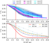 |
Fig. 8 Upper panel: radial profile of the emission of cores #1 to #6 in the ALMA 219 GHz 7M+TM2 continuum images. Lower panel: radial profile of the emission expected from isothermal cores with a known radial density distribution observed with the resolution of ALMA 219 GHz 7M+TM2 data. We report the observed profiles of cores #1, #4, and #5 for visual comparison. The dashed vertical red line indicates the beam half width at half maximum of the 219 GHz continuum data. |
4.2 Evolutionary stages of the cores from chemistry
The enhancement in the abundance of N2D+ and DCO+is associated with early stages of star formation, where the freeze-out of the CO onto dust grains at densities above 105 cm−3 and temperatures below 20 K removes the main destruction pathways of the H2D+ ion, and starts the deuteration process (Millar et al. 1989; Caselli & Ceccarelli 2012; Fontani et al. 2011). This is not the case for DCN, which is often found to be more abundant in warmer gas, thanks to chemical pathways that are efficient at higher temperatures (Millar et al. 1989; Roueff et al. 2007; Parise et al. 2009; Gieser et al. 2021; Cunningham et al. 2023).
Fontani et al. (2011) show that deuterium fractionation from N2H+ is extremely sensitive to gas temperature, and high-mass starless cores with warmer temperatures (above 20 K) have a drop of one order of magnitude in the D/H ratio. The extreme dependence on gas temperature is also evident in the models presented in Fontani et al. (2014), which shows that after the temperature increases above 20 K the D/H ratio drops after just ~102 yr for N2H+ and after ~104 yr for HNC. The timescale of the drop in the D/H ratio for DCO+is similar to that of N2D+(~100 yr), as it is possible to see in Fig. B.1 in the appendix. The plot shows the result of the same model run in Fontani et al. (2014) for a density of 105 cm−3 (private communication with K. Furuya and F. Fontani).
We indeed found that three out of four disappearing cores (#2, #5, and #6) show bright and compact emission of DCO+(2–1) and N2D+(2–1). Since the enhancement of abundance of these species due to deuterium fractionation fades quickly with the onset of star formation and the subsequent rise in temperature above 20 K, we confirm that these are prestellar cores in a region of clustered star formation. This is further supported by the shallower radial profiles shown for all these cores, with the exception of core #6. Moreover, none of these cores is associated with SiO (5–4) emission, an outflow tracer, as is shown in Fig. C.1.
The lack of peaked emission in DCO+ and N2D+toward both cores #3 and #4 indicates that these cores have a higher temperature. Moreover, these two sources have a more peaked radial profile, since they are detected in the continuum as compact sources in ALMAGAL 7M+TM2+TM1, and as is shown in Sect. 4.1. Core #4 also shows bright and peaked emission of DCN, whose production is more effective in warmer gas, of CH3CCH, which is a complex organic molecule, also associated with more evolved stages of the star-formation process (Herbst & van Dishoeck 2009; Molinari et al. 2016; Sabatini et al. 2021), and of SiO, an outflow tracer. For this core we used the detected emission of CH3CCH (9–8) to derive a temperature of 39 ± 5 K. To summarize the information from the molecular emission toward core #4, DCO+ and N2D+, tracers of early stages of star formation, are not enhanced toward this source, while there is bright emission of DCN, CH3CCH, and SiO, the emission of which requires more evolved stages with higher temperatures, not seen in any other core. Therefore, we conclude that core #4 is the most chemically evolved one and we assume that the temperature in the rest of the cores along the arch is lower than toward core #4. Cores #7, #8, and #9 do not have peaked emission in DCO+(2–1) or N2D+(2–1), but cores #7 and #8 have been detected with a peaked morphology in DCN (2–1). For these reasons, we consider them and core #3 as in an intermediate evolutionary stage between that of cores #2, #5, and #6, and that of the most evolved core in our sample, namely core #4. Based on this, we assign a plausible range of temperatures between 10 K and 20 K to cores #2, #5, and #6, and a warmer range of between 20 K and 30 K to cores #3, #7, #8, and #9.
4.3 Mass estimates and virial parameter
To estimate the core masses, we used the equation
![Mathematical equation: $\[M=\frac{100 F_{\mathrm{INT}} D^2}{B_\nu(T) \kappa_\nu},\]$](/articles/aa/full_html/2026/05/aa58787-25/aa58787-25-eq4.png) (3)
(3)
where FINT is the integrated flux density derived from CuTEx at 219 GHz for cores from #2 to #6 and at 150 GHz for cores #7 to #9, D is the distance of the source, Bν(T) is the Planck function either at 219 GHz or 150 GHz for the core dust temperature T, the factor 100 is the usually assumed gas-to-dust ratio, and κν is the dust mass absorption coefficient, assumed to be 0.9 cm2 g−1 at 219 GHz as in Coletta et al. (2025), and scaled with a β of 1.7 to derive the dust opacity coefficient at 150 GHz, following the relation
![Mathematical equation: $\[\kappa_{150}=\kappa_{219}\left(\frac{150 ~\mathrm{GHz}}{219 ~\mathrm{GHz}}\right)^\beta.\]$](/articles/aa/full_html/2026/05/aa58787-25/aa58787-25-eq5.png)
For core #4 we used as the dust temperature the temperature estimated from the fit of CH3CCH, assuming that gas and dust are coupled. For the other cores, under the same assumption, we used the ranges of temperature defined in Section 4.2. We derived the mass ranges for those temperature ranges, and we listed them in Table 2. For these calculations we used the usually adopted gas-to-dust ratio of 100, but as is highlighted by the work of Giannetti et al. (2017) this ratio reaches higher values in the outer Galaxy, even though the data show a large scatter. In particular, at the galactocentric distance of AG286.0716–1.8229(~10 kpc) the gas-to-dust ratio from the relation found in Giannetti et al. (2017) would be of ~200. Thus, these masses could be underestimated up to a factor of two from the uncertainties on this parameter.
In Table 2 we also list an average FWHM from fits to all the molecular lines detected on the cores (listed in Table 3), obtained with a Gaussian fit of the mean spectrum over the size of each core. The fit to derive the FWHM for the three deuterated species reported in Table 3 does not take into account the hyperfine splitting of the lines; therefore, these are upper limits of the FWHM value. We did not consider the hyperfine splitting because only in a few cases were more transitions other than the main one detected in the spectrum, therefore the results of the fit including the hyperfine splitting were poorly constrained. With this information we can derive the virial parameter of the cores, αvir, defined as in (Bertoldi & McKee 1992):
![Mathematical equation: $\[\alpha_{\mathrm{vir}}=\frac{2 ~E_{\mathrm{kin}}}{E_{\mathrm{grav}}}=\frac{5 \sigma^2 ~r}{G ~M},\]$](/articles/aa/full_html/2026/05/aa58787-25/aa58787-25-eq6.png) (4)
(4)
where Ekin and Egrav are the kinetic and gravitational potential energy of the cores, while σ is the velocity dispersion, related to the FWHM by σ = FWHM/2.35. The values are reported in Table 2 and vary between 0.3 and 2.4 for all cores except core #7, which has a virial parameter larger than 3. Despite the large ranges due to uncertainties in the temperature, and therefore mass, of the cores, all the cores except for core #7 are consistent with bound objects (αvir < 2, e.g. Kauffmann et al. 2013), not only cores #3 and #4 that already have a central condensation at ~1400 au. Moreover, as was stated above, the FWHM and therefore σ for most of the cores are upper limits of the real value, since we did not take into account the hyperfine splitting, while the masses could be lower limits if the real gas-to-dust ratio in the region is above 100. Therefore the values of αvir reported here are also upper limits.
5 Testing the hypothesis of triggered star formation
The presence of an H II region in our FoV and the location of the cores in an arched-shaped region centered at the H II region does not ensure that these cores are the result of triggered star formation, as was found by Zhang et al. (2024). In the case of source AG286.0716–1.8229, we also see from Fig. 2 that there is a gap between the 23 cm emission and the dust and gas arched structure, with no evidence of a photodissociation region (PDR), such as a bright rim in the images of IRAC band 1 at 3.6 μm (see Fig. D.1) due to the emission of polycyclic aromatic hydrocarbons (PAHs), while the data from IRAC band 3 and 4 are not available and other typical molecular tracers of PDRs (see e.g. Kim et al. 2020) are not present in our data. One possibility is that the H II region is more extended than the region emitting at 23 cm (Kim & Koo 2001; Kurtz 2002), but the outer part of the H II is not efficiently emitting, due to possible lower values of the electron density or electron temperature. Another possibility is that the region is shaped not only by the H II region, but also by the presence of stellar winds (see e.g. Kim et al. 2025).
In both cases, to test if the formation of these cores is triggered, we compared the scale of fragmentation and the typical mass of fragments along the arch with the value expected in the case of a shell fragmentation as prescribed by the collect and collapse process. The formulae to calculate these parameters were derived by Whitworth et al. (1994):
![Mathematical equation: $\[\lambda_{\text {shell}} \sim 0.83\left(\frac{c_s}{0.2 \mathrm{km} / \mathrm{s}}\right)^{18 / 11}\left(\frac{N_{\mathrm{Ly}}}{10^{49} \mathrm{s}^{-1}}\right)^{-1 / 11}\left(\frac{n_0}{10^3 \mathrm{cm}^{-3}}\right)^{-5 / 11} ~\mathrm{pc},\]$](/articles/aa/full_html/2026/05/aa58787-25/aa58787-25-eq7.png) (5)
(5)
![Mathematical equation: $\[M_{\text {shell}} \sim 23\left(\frac{c_s}{0.2 \mathrm{km} / \mathrm{s}}\right)^{40 / 11}\left(\frac{N_{\mathrm{Ly}}}{10^{49} \mathrm{s}^{-1}}\right)^{-1 / 11}\left(\frac{n_0}{10^3 \mathrm{cm}^{-3}}\right)^{-5 / 11} ~\mathrm{M}_{\odot},\]$](/articles/aa/full_html/2026/05/aa58787-25/aa58787-25-eq8.png) (6)
(6)
![Mathematical equation: $\[R_{\text {shell}} \sim 5.8\left(\frac{c_s}{0.2 \mathrm{km} / \mathrm{s}}\right)^{4 / 11}\left(\frac{N_{\mathrm{Ly}}}{10^{49} \mathrm{s}^{-1}}\right)^{1 / 11}\left(\frac{n_0}{10^3 \mathrm{cm}^{-3}}\right)^{-6 / 11} ~\mathrm{pc},\]$](/articles/aa/full_html/2026/05/aa58787-25/aa58787-25-eq9.png) (7)
(7)
![Mathematical equation: $\[t_{\text {shell}} \sim 1.56\left(\frac{c_s}{0.2 \mathrm{km} / \mathrm{s}}\right)^{7 / 11}\left(\frac{N_{\mathrm{Ly}}}{10^{49} \mathrm{s}^{-1}}\right)^{-1 / 11}\left(\frac{n_0}{10^3 \mathrm{cm}^{-3}}\right)^{-5 / 11} ~\mathrm{yr},\]$](/articles/aa/full_html/2026/05/aa58787-25/aa58787-25-eq10.png) (8)
(8)
where λshell, Mshell, Rshell, and tshell are the characteristic scale of fragmentation, the characteristic mass of the fragments, and the radius of the shell at the time of fragmentation, tshell, respectively.
The only quantities needed to derive these parameters are the rate of ionizing photons, NLy ~ 6.2 × 1046phot. s−1, as derived in Sect. 3.2, the isothermal sound speed for the shell, cs, and the initial density of the material swept by the expanding H II region, n0, assuming that the mean density at clump scale observed is a good estimate of its initial value before the expansion of the H II region. We used the values derived from the Herschel infrared Galactic Plane Survey (Hi-Gal) (Elia et al. 2021), i.e., from the fit of the infrared SED at clump scale (~1 pc), for the temperature of the clump, its mass, and radius to derive the best estimate of cs and n0. Those are 0.2 km s−1 and 5.1×104cm−3, respectively. Using these values, and assuming a 10% error for all the three parameters in Eqs. (5)–(8), we find that λshell ~ 0.22 ± 0.05 pc, Mshell ~ 6 ± 3 M⊙, Rshell ~ 0.43 ± 0.04 pc, and tshell ~ 0.42 ± 0.05 Myr.
We list the separation of all the bound cores along the arch (i.e., all except core #7) in Table 4. The median value in AG286.0716–1.8229 is 0.25 ± 0.15 pc. However, this is a lower limit of the separation, assuming that all the cores are perfectly aligned on the plane of the sky. For a couple of randomly oriented sources in 3d, the average deprojection factor is 4/π (see Schisano et al. 2026). The mean deprojected value is 0.34 ± 0.19. We consider this value an upper limit for the mean separation, since from the disposition of the cores on a circular arch it is likely that the 3D structure is not randomly oriented, and the 3D separations do not have a large contribution in the direction perpendicular to the plane of the sky. Both the deprojected and the observed mean separation of the cores are compatible within the error with that expected from the collect and collapse scenario, with the deprojected value being a factor ~1.5 larger than the estimate for the model. The mean mass of the cores considering both the upper limits and the lower limits reported in Table 2 is 6 ± 4 M⊙. Therefore they are also compatible with the characteristic mass of Mshell ~ 6 M⊙, while Rshell ~ 0.4 pc is smaller than the radius of the arc of 0.75 pc, but within a factor of 2.
Assuming the same values of cs and NLy, a radius of ~0.75 pc from Eq. (7) corresponds to a value of the initial volume density before the expansion of the H II region n0 ~ 2 × 104 cm−3, only a factor of ~2.5 smaller than the value evaluated by Elia et al. (2021) for the current mean density of the clump. Using this new value of n0 the estimates from Eqs. (5), (6), and (8) would be λshell ~ 0.34 ± 0.08 pc, Mshell ~ 9 ± 4 M⊙, and tshell ~ 0.67 ± 0.08 Myr. The fragmentation scale and the typical mass of the fragments would still be compatible with the median values observed within their errors, differing from the observed values by a factor of ~1.1 and ~1.5, respectively.
We also compared the mean separation and mass of the fragments with the thermal Jeans length and the thermal Jeans mass, using the properties at the clump level. These were derived by Schisano et al. (2026) to be 0.10 pc and 1.7 M⊙, with an error of 0.01 pc and 0.4 M⊙ respectively, assuming a 10% error on the two parameters involved in their calculation, i.e., the volume density and the temperature of the gas, as is seen in Eqs. (B.2) and (B.3) of Schisano et al. (2026).
The thermal Jeans length is a factor of 2.5 lower than the mean observed separation, and a factor of 3.4 lower than the mean deprojected separation and not compatible within the errors. The thermal Jeans mass is a factor of ~3.5 lower than the mean of the masses observed. The thermal Jeans mass is marginally compatible within the error with the mean mass from observations (upper limit from the model: 1.7 + 0.4 = 2.1 M⊙; lower limit of the mean of the mass estimated 6 − 4 = 2 M⊙). Nevertheless, as is discussed in Sect. 4.3 the dust-to-gas ratio in this region could be higher than 100, leading to higher estimates of the masses observed.
Figure 9 summarizes the comparison between the observations and the models, showing that the observed separations and masses for the cores in AG286.0716–1.8229 are in agreement with predictions from the collect and collapse models.
Separation of the bound cores along the arch-shaped region.
6 Conclusions
To study the nature of the disappearing cores, i.e., cores identified as compact sources in the ALMAGAL 7M+TM2 continuum at ~5000 au (7600 au for AG286.0716–1.8229) with no counterpart in the ALMAGAL 7M+TM2+TM1 continuum at ~1000 au (1400 au for AG286.0716–1.8229), we collected archival continuum centimeter and infrared data and new molecular line observations of the source AG286.0716–1.8229, which is associated with a candidate H II region from the catalog of Anderson et al. (2014). Here we summarize the main results of our work:
We built the radial profiles of the emission of the cores in the ALMAGAL FoV and confirmed that the profiles of the disappearing cores are shallower than those of cores #3 and #4, except core #6. This core has a profile similar to those of core #3 and #4, which are also detected in the higher-resolution ALMAGAL images. The flux density radial profiles are compatible with the flux density expected for Bonnor-Ebert density profiles, with a larger inner flat region for the disappearing cores;
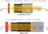
Fig. 9 Upper panel: mean observed separation in yellow and mean deprojected separation in orange. The black, gray, and red boxes represent the values derived from the collect and collapse model with n0 = 5.1 × 104 cm−3 (CC 1), with n0 = 2 × 104 cm−3 (CC 2), and from the thermal Jeans fragmentation model, respectively. Lower panel: Mean mass of the fragments in orange. The black, gray, and red boxes represent the values derived from the same models in the upper panel.
From the analysis of the radial profiles and of the emission of DCO+(2–1), N2D+(2–1), and SiO (5–4) we confirm that cores #2, #5, and #6 (i.e., three out of four disappearing cores) are young prestellar objects. The other disappearing core, core #1, does not have a compact morphology when observed in ALMA Band 4, and likely corresponds to material dispersed by the expansion of the H II region or the relic of the dust envelope around the ionizing star;
From the ~23 cm radio continuum emission, we inferred the spectral index between 0.8 GHz and 1.6 GHz, which is consistent with the flat index of optically thin free-free emission (α ~ −0.1 to −0.4). We therefore confirmed the presence of a H II region in this source. We derived a rate of ionizing photons, NLy ~ 6.2 × 1046 photons s−1, which corresponds to a B0.5 star;
The continuum emission in ALMA Bands 4 and 6 revealed a distribution of cores along an arch-shaped region that has a radius of ~0.75 pc, centered close to the peak of the 23 cm radio continuum emission;
From the chemical characterization of the cores we derived an evolution sequence among the cores and assigned a range of gas and dust temperatures. Only toward the most evolved core, #4, were we able to derive a precise measurement of the temperature (39±5 K), thanks to the detection of CH3CCH;
The virial parameter derived for all the cores in the arched structure is consistent with bound objects, with the exception of core #7;
We compared the separations of the cores along the arch structure and their typical masses with the characteristic separation and mass derived in the collect and collapse scenario and with the thermal Jeans length and mass. The best agreement is found with the characteristic scales in the case of triggered star formation.
This study confirmed that disappearing cores are good prestellar core candidates. The presence of several of these cores in the ALMAGAL sample will allow us to improve the statistics and study how these early stages are affected by the feedback of already formed massive stars.
Acknowledgements
The authors thank K. Furuya for the plot that shows the result for DCO+of the D/H drop after the temperature increase in the model presented in Fontani et al. (2014). The authors thanks the referee for their insightful comments. C.M. and the INAF-IAPS team acknowledge funding from the European Research Council (ERC) under the European Union’s Horizon 2020 program through the ECOGAL Synergy grant (ID 855130). CM acknowledges funding from INAF Mini Grants RSN2 2024 “Zodyac” CUP C83C25000340005. RK acknowledges financial support via the Heisenberg Research Grant funded by the Deutsche Forschungsgemeinschaft (DFG, German Research Foundation) under grant no. KU 2849/9, project no. 445783058. Part of this research was carried out at the Jet Propulsion Laboratory, California Institute of Technology, under a contract with the National Aeronautics and Space Administration (80NM0018D0004). D.C.L. acknowledges financial support from the National Aeronautics and Space Administration (NASA) Astrophysics Data Analysis Program (ADAP). L.B. gratefully acknowledges support by the ANID BASAL project FB210003. A.S-M. acknowledges support from the PID2023-146675NB grant funded by MCIN/AEI/10.13039/501100011033, and by the programme Unidad de Excelencia María de Maeztu CEX2020-001058-M, as well as support from the RyC2021-032892-I grant funded by MCIN/AEI/10.13039/501100011033 and by the European Union ‘Next GenerationEU’/PRTR. RSK acknowledges financial support from the ERC via Synergy Grant “ECOGAL” (project ID 855130) and from the German Excellence Strategy via the Heidelberg Cluster “STRUCTURES” (EXC 2181 - 390900948). In addition RSK is grateful for funding from the German BMWE in project “MAINN” (funding ID 50OO2206), and from DFG and ANR for project “STARCLUSTERS” (funding ID KL 1358/22-1). This paper makes use of the following ALMA data: project code 2019.1.00195.L and 2023.1.01386.S. ALMA is a partnership of ESO (representing its member states), NSF (USA) and NINS (Japan), together with NRC (Canada), MOST and ASIAA (Taiwan), and KASI (Republic of Korea), in cooperation with the Republic of Chile. The Joint ALMA Observatory is operated by ESO, AUI/NRAO and NAOJ.
References
- Anderson, L. D., Bania, T. M., Balser, D. S., et al. 2014, ApJS, 212, 1 [Google Scholar]
- Arce, H. G., Borkin, M. A., Goodman, A. A., Pineda, J. E., & Beaumont, C. N. 2011, ApJ, 742, 105 [NASA ADS] [CrossRef] [Google Scholar]
- Balser, D. S., Rood, R. T., Bania, T. M., & Anderson, L. D. 2011, ApJ, 738, 27 [NASA ADS] [CrossRef] [Google Scholar]
- Bertoldi, F. 1989, ApJ, 346, 735 [Google Scholar]
- Bertoldi, F., & McKee, C. F. 1992, ApJ, 395, 140 [NASA ADS] [CrossRef] [Google Scholar]
- Bonnor, W. B. 1956, MNRAS, 116, 351 [NASA ADS] [CrossRef] [Google Scholar]
- Burrell, P. M., Bjarnov, E., & Schwendeman, R. H. 1980, J. Mol. Spectrosc., 82, 193 [Google Scholar]
- Cacciapuoti, L., Macias, E., Maury, A. J., et al. 2023, A&A, 676, A4 [NASA ADS] [CrossRef] [EDP Sciences] [Google Scholar]
- CASA Team (Bean, B., et al.) 2022, PASP, 134, 114501 [NASA ADS] [CrossRef] [Google Scholar]
- Caselli, P., & Ceccarelli, C. 2012, A&A Rev., 20, 56 [NASA ADS] [Google Scholar]
- Caselli, P., Pineda, J. E., Zhao, B., et al. 2019a, ApJ, 874, 89 [NASA ADS] [CrossRef] [Google Scholar]
- Caselli, P., Pineda, J. E., Zhao, B., et al. 2019b, ApJ, 874, 89 [NASA ADS] [CrossRef] [Google Scholar]
- Cazzoli, G., & Puzzarini, C. 2008, A&A, 487, 1197 [Google Scholar]
- Coletta, A., Molinari, S., Schisano, E., et al. 2025, A&A, 696, A151 [NASA ADS] [CrossRef] [EDP Sciences] [Google Scholar]
- Cunningham, N., Ginsburg, A., Galván-Madrid, R., et al. 2023, A&A, 678, A194 [NASA ADS] [CrossRef] [EDP Sciences] [Google Scholar]
- Dale, J. E., Bonnell, I. A., & Whitworth, A. P. 2007, MNRAS, 375, 1291 [NASA ADS] [CrossRef] [Google Scholar]
- Deharveng, L., Lefloch, B., Kurtz, S., et al. 2008, A&A, 482, 585 [NASA ADS] [CrossRef] [EDP Sciences] [Google Scholar]
- Duchesne, S., Ross, K., Thomson, A. J. M., et al. 2025, PASA, 42, 38 [Google Scholar]
- Duchesne, S. W., Grundy, J. A., Heald, G. H., et al. 2024, PASA, 41, e003 [NASA ADS] [CrossRef] [Google Scholar]
- Ebert, R. 1955, ZAp, 37, 217 [Google Scholar]
- Elia, D., Massi, F., Strafella, F., et al. 2007, ApJ, 655, 316 [Google Scholar]
- Elia, D., Merello, M., Molinari, S., et al. 2021, MNRAS, 504, 2742 [NASA ADS] [CrossRef] [Google Scholar]
- Elmegreen, B. G., & Lada, C. J. 1977, ApJ, 214, 725 [Google Scholar]
- Endres, C. P., Schlemmer, S., Schilke, P., Stutzki, J., & Müller, H. S. P. 2016, J. Mol. Spectrosc., 327, 95 [NASA ADS] [CrossRef] [Google Scholar]
- Fischera, J. 2014, A&A, 571, A95 [NASA ADS] [CrossRef] [EDP Sciences] [Google Scholar]
- Fontani, F., Palau, A., Caselli, P., et al. 2011, A&A, 529, L7 [NASA ADS] [CrossRef] [EDP Sciences] [Google Scholar]
- Fontani, F., Palau, A., Busquet, G., et al. 2012, MNRAS, 423, 1691 [Google Scholar]
- Fontani, F., Sakai, T., Furuya, K., et al. 2014, MNRAS, 440, 448 [NASA ADS] [CrossRef] [Google Scholar]
- Giannetti, A., Leurini, S., König, C., et al. 2017, A&A, 606, L12 [NASA ADS] [CrossRef] [EDP Sciences] [Google Scholar]
- Gieser, C., Beuther, H., Semenov, D., et al. 2021, A&A, 648, A66 [EDP Sciences] [Google Scholar]
- Goedhart, S., Cotton, W. D., Camilo, F., et al. 2024, MNRAS, 531, 649 [CrossRef] [Google Scholar]
- Hale, C. L., McConnell, D., Thomson, A. J. M., et al. 2021, PASA, 38, e058 [NASA ADS] [CrossRef] [Google Scholar]
- Herbst, E., & van Dishoeck, E. F. 2009, ARA&A, 47, 427 [Google Scholar]
- Hosokawa, T., & Inutsuka, S.-i. 2005, ApJ, 623, 917 [NASA ADS] [CrossRef] [Google Scholar]
- Hunter, T. R., Indebetouw, R., Brogan, C. L., & et al. 2023, PASP, 135, 074501 [NASA ADS] [CrossRef] [Google Scholar]
- Kauffmann, J., Pillai, T., & Goldsmith, P. F. 2013, ApJ, 779, 185 [NASA ADS] [CrossRef] [Google Scholar]
- Kendrew, S., Simpson, R., Bressert, E., et al. 2012, ApJ, 755, 71 [NASA ADS] [CrossRef] [Google Scholar]
- Kendrew, S., Beuther, H., Simpson, R., et al. 2016, ApJ, 825, 142 [Google Scholar]
- Kim, K.-T., & Koo, B.-C. 2001, ApJ, 549, 979 [Google Scholar]
- Kim, W.-J., Wyrowski, F., Urquhart, J. S., et al. 2020, A&A, 644, A160 [NASA ADS] [CrossRef] [EDP Sciences] [Google Scholar]
- Kim, W.-J., Beuther, H., Wyrowski, F., et al. 2025, A&A, 694, A30 [Google Scholar]
- Kurtz, S. 2002, in Astronomical Society of the Pacific Conference Series, 267, Hot Star Workshop III: The Earliest Phases of Massive Star Birth, ed. P. Crowther, 81 [Google Scholar]
- Liu, H.-L., Wu, Y., Li, J., et al. 2015, ApJ, 798, 30 [Google Scholar]
- Martín, S., Martín-Pintado, J., Blanco-Sánchez, C., et al. 2019, A&A, 631, A159 [Google Scholar]
- Matsakis, D. N., Evans, II, N. J., Sato, T., & Zuckerman, B. 1976, AJ, 81, 172 [Google Scholar]
- McConnell, D., Hale, C. L., Lenc, E., et al. 2020, PASA, 37, e048 [Google Scholar]
- Millar, T. J., Bennett, A., & Herbst, E. 1989, ApJ, 340, 906 [NASA ADS] [CrossRef] [Google Scholar]
- Molinari, S., Schisano, E., Faustini, F., et al. 2011, A&A, 530, A133 [NASA ADS] [CrossRef] [EDP Sciences] [Google Scholar]
- Molinari, S., Merello, M., Elia, D., et al. 2016, ApJ, 826, L8 [Google Scholar]
- Molinari, S., Schisano, E., Faustini, F., et al. 2017, CUTEX: CUrvature Thresholding EXtractor, Astrophysics Source Code Library [record ascl:1708.018] [Google Scholar]
- Molinari, S., Schilke, P., Battersby, C., et al. 2025, A&A, 696, A149 [NASA ADS] [CrossRef] [EDP Sciences] [Google Scholar]
- Müller, H. S. P., Thorwirth, S., Bizzocchi, L., & Winnewisser, G. 2000, Z. Naturfor. A, 55, 491 [Google Scholar]
- Müller, H. S. P., Pracna, P., & Horneman, V.-M. 2002, J. Mol. Spectrosc., 216, 397 [Google Scholar]
- Palmeirim, P., Zavagno, A., Elia, D., et al. 2017, A&A, 605, A35 [NASA ADS] [CrossRef] [EDP Sciences] [Google Scholar]
- Panagia, N. 1973, AJ, 78, 929 [NASA ADS] [CrossRef] [Google Scholar]
- Parise, B., Leurini, S., Schilke, P., et al. 2009, A&A, 508, 737 [NASA ADS] [CrossRef] [EDP Sciences] [Google Scholar]
- Planck Collaboration XI. 2014, A&A, 571, A11 [NASA ADS] [CrossRef] [EDP Sciences] [Google Scholar]
- Redaelli, E., Bovino, S., Giannetti, A., et al. 2021, A&A, 650, A202 [NASA ADS] [CrossRef] [EDP Sciences] [Google Scholar]
- Roueff, E., Parise, B., & Herbst, E. 2007, A&A, 464, 245 [NASA ADS] [CrossRef] [EDP Sciences] [Google Scholar]
- Sabatini, G., Bovino, S., Giannetti, A., et al. 2021, A&A, 652, A71 [NASA ADS] [CrossRef] [EDP Sciences] [Google Scholar]
- Sánchez-Monge, Á., Brogan, C. L., Hunter, T. R., et al. 2025, A&A, 696, A150 [Google Scholar]
- Schisano, E., Molinari, S., Coletta, A., et al. 2026, A&A, 707, A221 [Google Scholar]
- Sharma, T., Chen, W. P., Panwar, N., Sun, Y., & Gao, Y. 2022, ApJ, 928, 17 [Google Scholar]
- Shu, F. H., Adams, F. C., & Lizano, S. 1987, ARA&A, 25, 23 [CrossRef] [Google Scholar]
- Tackenberg, J., Beuther, H., Plume, R., et al. 2013, A&A, 550, A116 [Google Scholar]
- Thompson, M. A., Urquhart, J. S., Moore, T. J. T., & Morgan, L. K. 2012, MNRAS, 421, 408 [NASA ADS] [Google Scholar]
- Walch, S., Whitworth, A. P., Bisbas, T. G., Hubber, D. A., & Wünsch, R. 2015, MNRAS, 452, 2794 [Google Scholar]
- Wang, Y., Audard, M., Fontani, F., et al. 2016, A&A, 587, A69 [Google Scholar]
- Wang, K.-S., Comrie, A., Harris, P., et al. 2020, in Astronomical Society of the Pacific Conference Series, 527, Astronomical Data Analysis Software and Systems XXIX, eds. R. Pizzo, E. R. Deul, J. D. Mol, J. de Plaa, & H. Verkouter, 213 [Google Scholar]
- Weingartner, J. C., & Draine, B. T. 2001, ApJ, 548, 296 [Google Scholar]
- Whitney, B., Benjamin, R., Churchwell, E., et al. 2011, Deep GLIMPSE: Exploring the Far Side of the Galaxy, Spitzer Proposal ID #80074 [Google Scholar]
- Whitworth, A. P., Bhattal, A. S., Chapman, S. J., Disney, M. J., & Turner, J. A. 1994, MNRAS, 268, 291 [Google Scholar]
- Zavagno, A., Deharveng, L., Comerón, F., et al. 2006, A&A, 446, 171 [NASA ADS] [CrossRef] [EDP Sciences] [Google Scholar]
- Zavagno, A., Pomarès, M., Deharveng, L., et al. 2007, A&A, 472, 835 [NASA ADS] [CrossRef] [EDP Sciences] [Google Scholar]
- Zavagno, A., Russeil, D., Motte, F., et al. 2010, A&A, 518, L81 [Google Scholar]
- Zhang, S., Liu, T., Wang, K., et al. 2024, MNRAS, 535, 1364 [Google Scholar]
- Zhou, J., Zhou, D., Esimbek, J., et al. 2020, ApJ, 897, 74 [NASA ADS] [CrossRef] [Google Scholar]
This is the typical value for the whole ALMAGAL sample. For source AG286.0716–1.8229 it is 1400 au.
This is the typical value for the whole ALMAGAL sample. For source AG286.0716–1.8229 it is 7600 au.
The best order for the background is automatically assessed by CuTEx.
The entry of CDMS for CH3CCH is based on the following works: Burrell et al. (1980); Müller et al. (2000, 2002); Cazzoli & Puzzarini (2008).
Appendix A Spectra averaged on the cores
For each cores detected in the ALMA data toward AG286.0716–1.8229, we extracted the average spectra for N2D+(2–1), DCO+(2–1), DCN (2–1), and CH3CCH (9–8). These are shown in Fig. A.1.
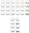 |
Fig. A.1 Spectra averaged over the cores (#2 to #9, each column corresponds to a core). The dashed horizontal line is 5 time the rms of the spectra. |
Appendix B D/H ratio drop timescale for DCO+
In Fig. B.1 we show the results of the model by Fontani et al. (2014) in the case of a density of 105 cm−3 (private communication with F. Fontani and K. Furuya).
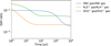 |
Fig. B.1 D/H ratio as a function of time after the temperature rises from 15 K to 40 K. |
Appendix C SiO moment maps
We created the moment-0 and moment-1 maps of SiO (5-4) in the ALMAGAL dataset using the same methodology described in Sect. 3.3. These are shown in Fig. C.1
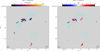 |
Fig. C.1 Moment-0 map (left) and moment-1 map (right) of the SiO (5–4) transition, from ALMAGAL data. The cyan ellipses represent the cores identified by CuTEx in the 219 GHz 7M+TM2 continuum data. |
Appendix D IRAC emission
In Fig. D.1 we show the emission at 3.6 and 4.5 μm from the Deep GLIMPSE survey observed by Spitzer Infrared Array Camera (IRAC) (Whitney et al. 2011) with ~ 2″ resolution. No data for the coordinates of source AG286.0716–1.8229 were available at 5.8 and 8.0 μm from the NASA/IPAC Infrared Science Archive (IRSA).
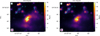 |
Fig. D.1 Emission at the coordinates of source AG286.0716–1.8229 in IRAC band 1 and band 2. The cyan contours are the contour of the continuum emission in ALMA Band 4 (4, 10, and 20 times the rms). The IRAC beam is shown in the bottom-left corner in purple, while the ALMA Band 4 beam is shown in cyan in the upper-left corner. |
All Tables
All Figures
|
Fig. 1 Top left panel: continuum emission at 150 GHz; the magenta circle represents the FoV of the ALMAGAL observations, while the dashed white circle visually represent the arch-shaped region where the continuum cores are detected. Top middle panel: ALMAGAL 7M+TM2 continuum emission; the cyan boxes are the footprint of the zoom-ins in the lower panels. Top right panel: ALMAGAL 7M+TM2+TM1 continuum emission. The dashed white circle in all the three top panels visually represents the 0.75 pc radius circle along which all cores, except core #1, are aligned. Lower panel: zoom-ins of the regions delimited in cyan in the top middle panel, where we kept the same color scale for the three different datasets. The cyan ellipses represent the compact sources identified with CuTEx in the ALMAGAL 7M+TM2 data, with their identification number reported in cyan, while the black ellipses and the green ellipses are the compact sources identified with CuTEx in the ALMA Band 4 data and the ALMAGAL 7M+TM2+TM1 data, respectively. |
| In the text | |
|
Fig. 2 Radio emission at 23 cm from the SMGPS in color scale (units millijansky/beam), with overimposed cyan contours (4,10, and 20 times the rms) of the ALMA Band 4 continuum emission at 150 GHz. The beam of the 23 cm emission is shown in purple in the bottom left corner. The beam of the ALMA 150 GHz emission is shown in cyan in the upper left corner. |
| In the text | |
|
Fig. 3 Spectral energy distribution of the radio emission between 0.88 GHz and 219 GHz from SMGPS, RACS, ALMAGAL, and the new data presented in this paper. The dashed green line is the best linear fit between 0.88 and 1.65 GHz including all the data points; the dashed red line is the best linear fit between 0.88 and 1.65 GHz if the SMGPS point at 1.65 GHz is removed; the dashed purple line is the best fit of the 150 and 219 GHz flux, after removing the free-free contamination assuming the green fit; and the dashed yellow line is the same as the purple one, but calculating the free-free contamination using the dashed red line. |
| In the text | |
|
Fig. 4 Top panel: moment-0 map of DCO+(2–1) (left), N2D+(2–1) (middle), and DCN (2–1) (right). Bottom panels: zooms-in of the three moment-0 maps in the boxes delimited in cyan in the upper panels. The cyan and white ellipses identify the compact cores extracted with CuTEx from the ALMAGAL 7M+TM2 continuum and ALMA Band 4 continuum, respectively. Some of the zoom-in boxes have the intensity multiplied by a factor reported in red in the top right corner of the box, to highlight the emission with respect to the color scale adopted for the full maps. |
| In the text | |
|
Fig. 5 Moment-1 (left) of DCO+(2–1) and FWHM (right) from the fit pixel by pixel of the line profile of DCO+(2–1). The color scales unit is km s−1. The dashed line boxes are the same as in Fig. 1. The cyan ellipses are the compact cores detected. The dashed white circle is the 0.75 pc radius circle along which the cores are aligned. |
| In the text | |
|
Fig. 6 Left panel: moment-0 maps of DCO+(2–1) with shown in white the cuts for the PV plots, centered at the peak positions of the cores. Right panels: PV plots for each core in the arch. The vertical white line delimits the position of the peak of the core. The dashed magenta line delimits the contours where the emission is half and two thirds of the maximum. |
| In the text | |
|
Fig. 7 Average spectrum of CH3CCH (9–8) over core #4 in black. In red we show the simulated spectrum obtained using the best-fit parameters with MADCUBA. |
| In the text | |
|
Fig. 8 Upper panel: radial profile of the emission of cores #1 to #6 in the ALMA 219 GHz 7M+TM2 continuum images. Lower panel: radial profile of the emission expected from isothermal cores with a known radial density distribution observed with the resolution of ALMA 219 GHz 7M+TM2 data. We report the observed profiles of cores #1, #4, and #5 for visual comparison. The dashed vertical red line indicates the beam half width at half maximum of the 219 GHz continuum data. |
| In the text | |
|
Fig. 9 Upper panel: mean observed separation in yellow and mean deprojected separation in orange. The black, gray, and red boxes represent the values derived from the collect and collapse model with n0 = 5.1 × 104 cm−3 (CC 1), with n0 = 2 × 104 cm−3 (CC 2), and from the thermal Jeans fragmentation model, respectively. Lower panel: Mean mass of the fragments in orange. The black, gray, and red boxes represent the values derived from the same models in the upper panel. |
| In the text | |
|
Fig. A.1 Spectra averaged over the cores (#2 to #9, each column corresponds to a core). The dashed horizontal line is 5 time the rms of the spectra. |
| In the text | |
|
Fig. B.1 D/H ratio as a function of time after the temperature rises from 15 K to 40 K. |
| In the text | |
|
Fig. C.1 Moment-0 map (left) and moment-1 map (right) of the SiO (5–4) transition, from ALMAGAL data. The cyan ellipses represent the cores identified by CuTEx in the 219 GHz 7M+TM2 continuum data. |
| In the text | |
|
Fig. D.1 Emission at the coordinates of source AG286.0716–1.8229 in IRAC band 1 and band 2. The cyan contours are the contour of the continuum emission in ALMA Band 4 (4, 10, and 20 times the rms). The IRAC beam is shown in the bottom-left corner in purple, while the ALMA Band 4 beam is shown in cyan in the upper-left corner. |
| In the text | |
Current usage metrics show cumulative count of Article Views (full-text article views including HTML views, PDF and ePub downloads, according to the available data) and Abstracts Views on Vision4Press platform.
Data correspond to usage on the plateform after 2015. The current usage metrics is available 48-96 hours after online publication and is updated daily on week days.
Initial download of the metrics may take a while.