


| Issue |
A&A
Volume 710, June 2026
|
|
|---|---|---|
| Article Number | A56 | |
| Number of page(s) | 25 | |
| Section | Extragalactic astronomy | |
| DOI | https://doi.org/10.1051/0004-6361/202558627 | |
| Published online | 28 May 2026 | |
AGILE: An end-to-end Rubin-LSST simulation of active galactic nuclei, galaxies, and stars
I. Software description and first data release
1
University of Bristol, Via Frascati 33, 00078, Monteporzio Catone, Italy
2
Department of Astronomy, University of Geneva, ch. d’Ecogia 16, 1290, Versoix, Switzerland
3
Department of Physics, University of Helsinki, Gustaf Hällströmin katu 2, 00014, Helsinki, Finland
4
School of Physics, HH Wills Physics Laboratory, University of Bristol, Tyndall Avenue, Bristol, BS8 1TL, UK
5
INAF–Osservatorio Astronomico di Padova, Vicolo dell’Osservatorio 5, I-35122, Padova, Italy
6
Dipartimento di Fisica “Ettore Pancini”, Università degli Studi di Napoli Federico II, Via Cintia, 80126, Napoli, Italy
7
INAF–Osservatorio Astronomico di Capodimonte, Via Moiariello 16, 80131, Napoli, Italy
8
School of Physics and Astronomy, University of Southampton, Highfield, Southampton, SO17 1BJ, UK
9
Scuola Normale Superiore, Piazza dei Cavalieri 7, 56126, Pisa, Italy
10
University of Belgrade-Faculty of Mathematics, Department of Astronomy, Studentski trg 16, 11000, Belgrade, Serbia
11
Hamburger Sternwarte, Universität Hamburg, Gojenbergsweg 112, D-21029, Hamburg, Germany
12
Istituto Nazionale di Fisica Nucleare (INFN) – Sez. di Napoli, Compl. Univ. di Monte S. Angelo, Edificio G, Via Cinthia, I-80126, Napoli, Italy
13
Dipartimento di Fisica e Astronomia “Galileo Galilei”, Università di Padova, Vicolo dell’Osservatorio 3, I-35122, Padova, Italy
14
Department of Physics and Astronomy “Augusto Righi”, University of Bologna, Via Gobetti 93/2, 40129, Bologna, Italy
15
Department of Physics and Astronomy, Wayne State University, Detroit, MI, 48202, USA
16
Instituto de Estudios Astrofísicos, Facultad de Ingeniería y Ciencias, Universidad Diego Portales, Av. Ejército Libertador 441, Santiago, Chile
17
Department of Astronomy and Astrophysics, 525 Davey Laboratory, The Pennsylvania State University, University Park, PA, 16802, USA
18
Institute for Gravitation and the Cosmos, The Pennsylvania State University, University Park, PA, 16802, USA
19
Department of Physics, 104 Davey Laboratory, The Pennsylvania State University, University Park, PA, 16802, USA
20
Centre for Astrophysics and Supercomputing, Swinburne University of Technology, Hawthorn, VIC, 3122, Australia
21
Kavli Institute for Astronomy and Astrophysics, Peking University, Beijing, 100871, People’s Republic of China
22
National Astronomical Observatories, Chinese Academy of Sciences, 20A Datun Road, Beijing, 100101, People’s Republic of China
23
Universidade Federal de Santa Maria (UFSM), Centro de Ciências Naturais e Exatas (CCNE), Santa Maria, 97105-900, RS, Brazil
24
Eureka Scientific, 2452 Delmer Street, Suite 100, Oakland, CA, 94602-3017, USA
25
Department of Physics, Yale University, PO Box 208120, New Haven, CT, 06520, USA
26
INAF, Osservatorio Astrofisico di Torino, Via Osservatorio 20, I-10025, Pino Torinese, Italy
27
NASA Goddard Space Flight Center, Greenbelt, MD, 20771, USA
28
Center for Space Science and Technology, University of Maryland Baltimore County, MD, 21250, Baltimore, USA
29
Korea Astronomy and Space Science Institute, 776 Daedeokdae-ro, Yuseong-gu, Daejeon, 30455, Republic of Korea
30
Department of Physics, Drexel University, 32 S. 32nd Street, Philadelphia, PA, 19104, USA
31
Max-Planck-Institut für extraterrestrische Physik, Giessenbachstr. 1, 85748, Garching, Germany
32
Exzellenzcluster ORIGINS, Boltzmannstr. 2, D-85748, Garching, Germany
33
Centre for Extragalactic Astronomy, Department of Physics, Durham University, South Road, Durham, DH1 3LE, UK
34
Physics Department, Tor Vergata University of Rome, Via della Ricerca Scientifica 1, 00133, Rome, Italy
35
INFN – Rome Tor Vergata, Via della Ricerca Scientifica 1, 00133, Rome, Italy
36
National Radio Astronomy Observatory, 520 Edgemont Rd, Charlottesville, VA, 22903, USA
37
Department of Astronomy, University of Virginia, PO Box 3818, Charlottesville, VA, 22903, USA
38
Department of Astronomy, University of Michigan, 1085 South University, Ann Arbor, MI, 48109, USA
★ Corresponding author: This email address is being protected from spambots. You need JavaScript enabled to view it.
Received:
17
December
2025
Accepted:
11
March
2026
Abstract
Aims. Contemporary large-scale surveys such as the Vera C. Rubin Observatory Legacy Survey of Space and Time (LSST) and Euclid present an unprecedented discovery potential for studying active galactic nuclei (AGNs) at the population level in the big data era. However, one major challenge is the accurate identification and classification of AGNs from optical and near-infrared photometry or variability data alone. To optimize active galactic nucleus (AGN) selection, classification, and systematics as well as to test different data analysis tools, we present AGILE (AGNs In the LSST Era), an LSST end-to-end simulation software. Developed as part of the INAF LSST in-kind contribution, AGILE is capable of simulating the anticipated AGN population in LSST and Euclid.
Methods. We based AGILE on existing simulations of galaxies and stars, while we developed an AGN recipe based on empirical relations. AGILE populates complete galaxy samples with AGNs according to the observed AGN accretion rate distribution, and each AGN is assigned an optical/UV spectral energy distribution. Optical AGN variability is added using a damped random walk model connected to the AGN physical parameters. Finally, AGILE creates both LSST-like images and related data products.
Results. Using AGILE, we built a 24 deg2 complete mock truth catalog of AGNs, galaxies, and stars with 0.2 < z < 5.5, log10(Mstar/M⊙) > 8.5 (AGNs and galaxies), and r < 27.5 mag (stars). We also performed a pilot simulation (AGILE DR1) consisting of 1 deg2 of LSST operations in the COSMOS field observed up to three years in accordance with the survey strategy. We used AGILE DR1 to quantify the accuracy of the LSST Science Pipelines in recovering the true fluxes of AGNs, galaxies, and stars. We quantified the LSST completeness and purity in recovering Type 1 AGNs using typical color-color and variability selections. We share the AGILE DR1 dataset, as it represents an ideal test bench for further scientific exploitation and forecasts in the context of LSST AGNs.
Key words: galaxies: active / quasars: general
© The Authors 2026
 Open Access article, published by EDP Sciences, under the terms of the Creative Commons Attribution License (https://creativecommons.org/licenses/by/4.0), which permits unrestricted use, distribution, and reproduction in any medium, provided the original work is properly cited.
This article is published in open access under the Subscribe to Open model. This email address is being protected from spambots. You need JavaScript enabled to view it. to support open access publication.
1. Introduction
The presence of a supermassive black hole (SMBH) with a mass in the range of log10(MBH/M⊙) ≈ 5–10 at the centers of massive galaxies is an accepted paradigm in astronomy (e.g., Kormendy & Richstone 1995; Kormendy & Bender 2011). These black holes grow by mergers and the accretion of gas and dust, the latter of which gives rise to the highly energetic phenomena observed in active galactic nuclei (AGNs; e.g., Lynden-Bell 1969; Alexander & Hickox 2012). Given the strong correlations between the properties of galaxies and their central SMBHs (Magorrian et al. 1998; Ferrarese & Merritt 2000; Kormendy & Ho 2013; Graham 2016, but see also Maiolino et al. 2024 for the z > 4 Universe), understanding the role of AGNs is crucial for building a comprehensive picture of galaxy evolution.
In the coming years, large-scale surveys such as the Vera C. Rubin Observatory Legacy Survey of Space and Time (LSST; Ivezić et al. 2019), Euclid (Euclid Collaboration: Mellier et al. 2025), eROSITA (Merloni et al. 2012), and others will usher AGN science into the era of big data. These surveys are expected to detect AGNs numbering in the tens of millions, vastly expanding on existing samples. However, a major challenge will be identifying these AGNs among the billions of sources (primarily galaxies) that will be detected by these surveys. Thus, the ability to perform reliable AGN selection based on optical and near-infrared (NIR) photometry and variability will be a fundamental goal (e.g., Savić et al. 2023; Euclid Collaboration: Matamoro Zatarain et al. 2025). To prepare for these surveys, it is essential to develop synthetic datasets that can serve as test beds for selection methodologies, completeness estimates, and data analysis tools such as variability detection, morphology classification, and photometric redshift estimation.
Approximately 18 000 deg2 of the southern extragalactic sky will be covered by LSST for ten years. With six photometric bands (ugrizy) and hundreds of repeated observations per region, the high-cadence imaging of LSST will be a transformative tool for AGN research, particularly for variability studies. While LSST is expected to select a high-purity sample of some ten million AGNs in the optical regime, AGNs detected by LSST is at least an order of magnitude larger (LSST Science Collaboration 2009; Li et al. 2025a). At the same time, Euclid will provide a complementary view of the LSST sky with space-based optical/NIR imaging (IE < 24.5, HE < 24) and NIR spectroscopy (R = 380). This will be especially helpful in uncovering the obscured AGN population (e.g., Euclid Collaboration: Matamoro Zatarain et al. 2025; Euclid Collaboration: Tarsitano et al. 2025).
In preparation for the massive LSST dataset, we introduce AGNs In the LSST Era (AGILE), an end-to-end simulation pipeline developed as part of the Italian Istituto Nazionale di Astrofisica (INAF) in-kind contribution to LSST. AGILE is designed to generate realistic AGN catalogs and simulate their observational properties as seen by LSST, thus enabling robust testing and optimization of AGN selection and classification strategies as well as of a broad range of data analysis tools. A similar work was conducted by the Rubin-LSST Dark Energy Science Collaboration (DESC; Korytov et al. 2019; Dark Energy Science Collaboration 2021); however, neither AGNs nor high-redshift galaxies were accounted for. The AGILE software is designed to complement the work of DESC by providing a complete census of the AGN population.
In Sect. 2, we present an overview of AGILE. In Sect. 3, we describe the generation of the galaxy catalogs, and this is followed by the AGN population model being presented in Sect. 4 and the stellar catalog being shown in Sect. 5. We report the validation results of the AGN catalog in Sect. 6 and the selected AGN and stellar variability recipes in Sect. 7. In Sect. 8 we describe the LSST-like image simulations, and in Sect. 9 we outline the generation of photometric catalogs. Science applications are discussed in Sect. 10, and this is followed by a summary and our conclusions in Sect. 11. Appendix D presents the AGILE data release 1 (DR1). The AGILE DR1 consists of a 24 deg2 truth catalog and a total of 1441 simulated visits in the ugrizy bands for a total of 21 (out of a total of 189) LSSTCam detectors covering the central 1 deg2 for the first three years of the survey. Throughout this work, we assume a flat Lambda cold dark matter cosmology with Ωm = 0.3 and H0 = 70 km s−1 Mpc−1 (Wilkinson Microwave Anisotropy Probe; Spergel et al. 2003)1 and the Chabrier (2003) initial mass function. Magnitudes are expressed in the AB system (Oke & Gunn 1983).
2. AGILE overview
AGILE first builds a mock catalog including AGNs, galaxies, and stars based on empirical relations, ensuring consistency with observed AGN and galaxy properties. The strength of the empirical approach is to accurately reproduce the known underlying AGN population, which can then be directly compared to the recovered AGN population by the LSST strategy, primarily characterized by its large survey area and cadence. Moreover, this method follows the well-established methodology in the literature, which in recent years has been successful in explaining the large-scale clustering of AGNs in the context of selection effects from X-ray surveys (Comparat et al. 2019; Aird & Coil 2021; Allevato et al. 2021; Viitanen et al. 2021; López-López et al. 2024). Here, instead we focus on the optical properties of X-ray AGNs and quasars2 in the context of LSST, simulating as accurately as possible the effects of both the hardware (the telescope and the LSSTCam instrument) and the software (image processing pipelines). Therefore, AGILE includes a model for the instrumental effects, survey design, and time-domain variability for all sources. This enables a dynamic, evolving representation of the AGN population, as it will be observed by LSST, thus providing an essential framework for optimizing AGN detection and classification.
Figure A.1 shows the full AGILE flowchart, which can be divided into three main steps: the first step involves generating an empirically motivated mock truth catalog, where galaxies host X-ray AGNs following the latest accretion rate distribution by Zou et al. (2024b, hereafter Z24). Further optical and ultraviolet (UV) properties are assigned using empirical recipes (e.g., Lusso et al. 2010; Merloni et al. 2014), and full UV, optical, and NIR spectral energy distributions (SEDs) are generated with QSOGEN (Temple et al. 2021). These AGN SEDs are then combined with the galaxy SEDs generated by EGG (Empirical Galaxy Generator; Schreiber et al. 2017) to derive photometry in the optical/NIR, including the LSST and Euclid bands. The second step involves creating time-dependent instance catalogs, where AGN and stellar variability are captured by the LSST observing cadence. Finally, the instance catalogs are processed through the LSST image simulations, generating realistic LSST-like single-visit images. These images are then coadded and analyzed using the LSST Science Pipelines, mimicking real survey operations and producing final photometric catalogs.
3. AGILE mock galaxy catalog
The starting point of AGILE is a complete (in terms of stellar mass Mstar and redshift z) population of galaxies. The galaxy sample was created using EGG (Schreiber et al. 2017), which is designed to generate realistic mock catalogs of galaxies with physical properties such as Mstar, star-formation rates (SFRs), and SEDs. EGG galaxies are calibrated to reproduce the observed number counts within the GOODS (Barro et al. 2019; Guo et al. 2013) and CANDELS fields (Grogin et al. 2011; Koekemoer et al. 2011), as well as the angular two-point correlation function as a function of Mstar and z using the Soneira & Peebles (1978) algorithm. Moreover, EGG galaxies are classified as either quiescent or star-forming based on the input galaxy stellar mass function (SMF).
For the AGILE simulation of galaxies, we based the input galaxy SMF on the COSMOS 2 deg2 field (Scoville et al. 2007). The latest COSMOS2020 catalog (Weaver et al. 2022) has a comparable depth to the LSST wide survey after ten years (r ∼ 27.5; Bianco et al. 2022). Here, we used the quiescent and star-forming galaxy SMFs, measured for 0.2 < z < 5.5 galaxies that are classified as quiescent and star-forming based on near ultraviolet (NUV), r, and J colors (Weaver et al. 2023). In the interest of having a complete galaxy sample as the starting point, we allowed galaxies to be simulated down to log10(Mstar/M⊙) = 8.5. This constitutes an extrapolation at higher z, as COSMOS2020 70% mass completeness limits at z = 1.2 and 5.5 are log10(Mstar/M⊙) = 8.5 and 9.5, respectively (Weaver et al. 2023, Sect. 3.3).
4. AGILE mock AGN catalog
Following the empirical approach, we assigned a realistic population of AGNs to the complete population of galaxies according to the observed distributions of AGN properties and scaling relations (e.g., Georgakakis et al. 2019; Aird & Coil 2021; Allevato et al. 2021; Viitanen et al. 2021; López-López et al. 2024). Starting from a specific accretion rate (λSAR ≡ LX / Mstar, where LX is the intrinsic 2–10 keV AGN luminosity) distribution function (Z24), we built a complete X-ray AGN population over a wide luminosity baseline LX ≳ 1041 erg s−1 and 0.2 < z < 5.5. We then converted it into a population of optical/NIR AGNs across different optical types (i.e., Type 1 or Type 2), and included AGN optical variability.
4.1. Accretion rate distribution
We started by assigning λSAR to each galaxy in the simulation by using the AGN λSAR distribution p(λSAR | Mstar, z, T) (i.e., the probability that a quiescent or star-forming galaxy T with Mstar at z hosts an AGN with LX), which is observationally constrained in many studies (Bongiorno et al. 2016; Georgakakis et al. 2017; Aird et al. 2018; Yang et al. 2018; Laloux et al. 2024; Z24). The λSAR distribution is strongly influenced by at least Mstar, z, and T, and there is evidence of further dependencies on host-galaxy SFR (e.g., Aird et al. 2019; Yang et al. 2019), compactness (e.g., Ni et al. 2021), or on AGN obscuration (e.g., Ricci et al. 2017; Laloux et al. 2024).
4.1.1. Compton-thin AGNs
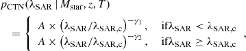
Here, we focus on reproducing the primary trends in the AGN-host galaxy connection in terms of Mstar, z, and T, and used the most recent measurements of the Compton-thin (CTN, neutral hydrogen column density NH < 1024 cm−2) pCTN(λSAR | Mstar, z, T) by Z24. Their sample spans 109.5 < Mstar/M⊙ < 1012 and z < 4, and is derived from a large selection of 8000 AGNs and 1.3 million non-active galaxies compiled from nine different XMM-Newton, Chandra, and eROSITA surveys with a wide reach in the area-depth plane (from 0.05 deg2 / 7000 ks to 59.75 deg2 / 2 ks). They find the observed pCTN(λSAR | Mstar, z, T) well-fitted by a double power-law with four free parameters: amplitude A, power-law slopes γ1, γ2, and λSAR, c marking the transition λSAR between the two power-law slopes.
For each galaxy in AGILE with a given Mstar, z, and T, we used the median model parameter maps shown in Fig. 2 of Z24 in order to find the corresponding parameters A, γ1, γ2, λSAR, c. Then, pCTN(λSAR | Mstar, z, T) was given by
 (1)
(1)
and we assigned each galaxy a value of λSAR drawn at random using the corresponding distribution. We extrapolated the parameter maps down to log10(Mstar/M⊙) = 8.5 and up to z = 5.5 by taking the boundary values of the parameter maps at log10(Mstar/M⊙) = 9.5 and z = 4, respectively. The choice of the extrapolation scheme affects pCTN(λSAR | Mstar, z, T) the most at z ≲ 0.5 (up to 2.0 dex), while the differences are < 0.5 dex at 0.5 < z < 4. We show these trends and discuss this further in Appendix B.
Recent observations suggest that the black-hole occupation fraction focc i.e., the probability of a galaxy hosting a SMBH could depend on Mstar (Miller et al. 2015; Burke et al. 2025; Zou et al. 2025). In particular, Zou et al. (2025), studying a sample of local (< 50 Mpc) galaxies, measure focc to be approximately 30%, 60%, and 100% at log10(Mstar/M⊙) = 8.5, 9.5, and 10.5, respectively. Given that focc is observationally constrained only in the local Universe, we did not account for it in the simulation where we assumed that every galaxy hosts a SMBH. However, focc was computed and a flag was provided for each galaxy in the truth catalog (see Sect. 6) and we verified that the validation results discussed in Sect. 6 hold also when focc is applied and extrapolated to any redshift.
Following Z24 and Aird et al. (2018), in AGILE a galaxy is defined to host an AGN, if λSAR > 1032 erg s−1 M⊙−1. Assuming a bolometric correction Lbol / LX = 25, and Mstar / MBH = 500, this corresponds approximately to an accretion rate of 1% Eddington (Aird et al. 2012; Bongiorno et al. 2016; Georgakakis et al. 2017). Using this cut, the AGN fraction is on the order of a few percent at z < 1.0 to a few tens of a percent at z > 1.0 (Z24, Fig. 7), which is in agreement with the observed AGN fraction of Aird et al. (2018).
4.1.2. Correcting for Compton-thick AGNs
It is important to note that Z24 derived results only for CTN AGNs. Indeed, while X-ray selection in the observed 2–10 keV band is among the most efficient ways of selecting AGNs, it is still biased against heavily obscured Compton-thick (CTK) AGNs with NH > 1024 cm−2. Given that X-ray background population synthesis models suggest that 30–50% of AGNs could be CTK (Ananna et al. 2019; Peca et al. 2023; Annuar et al. 2025) and mostly undetected by hard X-ray selection, we add in a correction for CTK AGNs.
To reproduce the CTK AGN number density as a function of LX and z, we used the AGN obscuration distribution function. Following Ueda et al. (2014), we defined f(NH | LX, z) (in units of dex−1) as the fraction of AGNs at a given NH, LX, and z. Then, the CTK AGN fraction is given by:
 (2)
(2)
Moreover, due to the lack of estimates of the accretion rate distribution of CTK AGNs (pCTK), given λSAR, Mstar, z, and T, we assumed that all AGNs are either CTN or CTK (pAGN = pCTN + pCTK), and that CTK AGNs relate to the total AGN population via pCTK = fracCTK × pAGN. Then, the CTK AGN accretion rate distribution is given by
 (3)
(3)
where LX = λSAR × Mstar, and we assumed pCTN from Z24. Consequently, the combined AGN accretion rate distribution is defined as pAGN = pCTN + pCTK, and the total AGN fraction is given by the integral
 (4)
(4)
where we defined λSAR, min = 1032 erg s−1 M⊙−1. We show the resulting accretion rate distributions of CTN and CTK AGNs in Fig. 1. For the CTK AGN occupation fraction (see Sect. 4), we chose to account for it by employing an identical recipe as for the CTN AGNs.
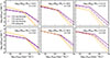 |
Fig. 1. Adapted distribution of λSAR of AGNs. Each panel shows p(λSAR | Mstar, z, T) at different Mstar (columns) and z (rows) values. The lines correspond to different combinations of AGN host galaxy type (quiescent or star forming) and AGN obscuration (CTN or CTK) in accordance with the legend. The specific Mstar and z values shown here have been selected for illustrative purposes, while the λSAR assignment follows the Z24 parameter maps as explained in Sect. 4.1. |
4.2. Supermassive black hole masses
The mass of the SMBH (MBH) is one of the most fundamental AGN properties. Tight correlations are observed between MBH and galaxy properties (velocity dispersion, luminosity, and Mstar; Magorrian et al. 1998; Gebhardt et al. 2000; Ferrarese 2002; Kormendy & Ho 2013), and discrepant scaling relations are known between early-type (merger-driven evolution) and late-type galaxies (e.g., Graham 2023, Fig. A4). In order to assign each AGN a MBH, we assumed the MBH–Mstar relation derived by using a novel method based on the continuity equation. In the continuity equation (e.g., Yang et al. 2018; Shankar et al. 2020b), galaxies were initially seeded with MBH at z = 5.5 following the local scaling relation (Reines & Volonteri 2015). Then, the growths of galaxies and BHs are governed by the evolution of the SMF and p(λSAR), which we based on COSMOS2020 (Weaver et al. 2023) and Z24, respectively. We assumed that accretion is the dominant channel of BH growth and ignored BH mergers, which has a negligible impact here apart from the local Universe and high-mass BHs. We further assumed a radiative and kinetic efficiency of 0.10 and 0.05, respectively (e.g., Soltan 1982; Shankar et al. 2020a). The strength of this method is that it produces a self-consistent BH population across different z, and the MBH–Mstar relation is a direct output of the simulation. This approach is favored to assuming an empirical z-dependent MBH–Mstar relation that has the downside of including any biases that are present in that particular measurement or galaxy population. We used the output MBH–Mstar relation from the continuity equation to assign each galaxy an MBH inclusive of an intrinsic scatter of ∼0.50 dex. (Reines & Volonteri 2015; Shankar et al. 2019)3. We show the resulting MBH–Mstar relation in Fig. 2.
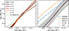 |
Fig. 2. Resulting MBH–Mstar scaling relation from the continuity equation. Left: z evolution of the scaling relations from z = 0 (darker) to z = 5 (lighter). At each redshift, the dashed line style indicates the regime above the 99% stellar mass limits (assuming Weaver et al. 2023 COSMOS2020 stellar mass function and an area of 24 deg2), above which the MBH − Mstar relation is to be considered an extrapolation. The dotted line shows the assumed initial conditions at z = 5.5 (Reines & Volonteri 2015). Right: Local relation implied by the continuity equation (black line). The shaded region corresponds to an assumed scatter of Δlog10(MBH/M⊙) = 0.50 dex. The other non-solid lines correspond to local and inactive early-type galaxies (Häring & Rix 2004; Kormendy & Ho 2013), local AGNs (Reines & Volonteri 2015), the de-biased relation from SDSS galaxies (Shankar et al. 2016), and major-merger built S0 and E galaxies (Graham 2023). |
As can be seen, the MBH–Mstar relation evolves rapidly from z = 5.5 to 5.0, indicating that the continuity equation implies a different overall MBH–Mstar relation to the initial conditions from Reines & Volonteri (2015). This rapid evolution at these z is a simulation artifact as in the continuity equation approach the initial conditions are quickly washed away. Then, the output MBH–Mstar relation settles quickly to the one implied by the continuity equation. Therefore, at these z the MBH values are to be considered unreliable. We further highlight the z-dependent 99% mass completeness limit (assuming COSMOS2020 and an area of 24 deg2) in Fig. 2 as dashed lines. In this regime, the MBH–Mstar relation may be considered an extrapolation.
4.3. Optical-UV properties: UV luminosity and AGN type
In order to derive realistic ugrizy photometry for the AGN population, we describe here our optical/UV model of the X-ray AGN population. First, we assigned each AGN a monochromatic UV luminosity L2500 Å based on the well-established relationship between L2500 Å and L2 keV (e.g., Just et al. 2007; Lusso et al. 2010; Lusso & Risaliti 2016)4. Starting from the intrinsic 2–10 keV luminosity, we derived the monochromatic 2 keV luminosity, assuming a standard power-law shape with Γ = 1.9 (e.g., Cappelluti et al. 2009). Then, we used the L2500 Å–L2 keV relation of Lusso et al. (2010, Eq. 5) for Type 1 AGNs in XMM-COSMOS. Finally, we factored in an intrinsic log-normal scatter of 0.40 dex in the L2500 Å, consistent with Lusso et al. (2010).
Only a fraction of the X-ray AGN population is expected to have optical/UV counterparts due to extinction by dust obscuration. To account for this, we assigned each AGN an optical classification between Type 1 (optically unobscured) and Type 2 (optically obscured). Here, we used the Type 2 AGN fraction as a function of LX and z based on XMM-COSMOS (Merloni et al. 2014). Moreover, we conservatively classified all CTK AGNs as Type 2. While the optical classification could be based on NH (e.g., Ueda et al. 2014), Merloni et al. (2014) do report on two AGN populations where the optical and X-ray classifications do not agree. These populations would be neglected in a scheme only based on NH.
4.4. Multiwavelength AGN spectral energy distribution
To generate the AGN SED templates, we used QSOGEN (Temple et al. 2021), which models the SED as the sum of various components representing the different AGN physical processes with a total of nine free parameters. These templates represent time-averaged SEDs and do not account for AGN variability, which we discuss in detail in Sect. 7.1. To briefly summarize the role of the parameters, QSOGEN models the accretion disk emission as a double power law, characterized by the spectral indices pslp1 and pslp2, with a break at the wavelength plbrk1.5 The NIR emission, originating from hot dust in the inner regions of the torus, is modeled as a black body with temperature TBB and normalization BB_norm. Broad emission lines are incorporated from composite spectra, with their intensity and equivalent width scaled via the parameters scal_emline and beslope, respectively. The host-galaxy emission is controlled by the parameters fragal and gpblind, where fragal defines the AGN-to-host flux fraction, and gpblind its dependence on AGN luminosity.
The posterior distribution of the free parameters is obtained by fitting the colors of quasi-stellar objects (QSOs) as a function of z. For each set of parameters, a SED is generated, from which synthetic colors are computed across different z, accounting also for intergalactic medium (IGM) absorption (Becker et al. 2013). These synthetic colors are then fitted against the observed data.
Notably, the best-fit parameters in Temple et al. (2021) are calibrated against a mixed population of quasars and AGNs with significant host-galaxy contamination. Instead, our chosen methodology of populating galaxies with AGNs requires a pure AGN SED to be added on top of the galaxy one. Thus, we followed a similar approach to the one used by Buchner et al. (2024) for the construction of the Chimera QSO benchmark, and we restricted the original sample to luminous quasars with L5100 Å ≥ 1045.5 erg s−1. This sample may be considered devoid of host-galaxy contamination (e.g., Shen et al. 2011), and it allowed us to derive pure AGN SED templates. We note that a potential limitation in our approach is that our sample is biased toward luminous high-Eddington accreting sources. As a result, the derived SED may not be fully representative of lower luminosity, low-accretion rate AGN, which are known to exhibit different SED shapes due to their distinct accretion regimes (e.g., López et al. 2024)
We started with the Temple et al. (2021) QSO sample from the SDSS Quasar DR16 catalog (Lyke et al. 2020) crossmatched with the UKIDSS Large Area Survey catalog (Lawrence et al. 2012) and the unWISE catalog (Schlafly et al. 2019). Out of 95 684 QSOs that are detected in all the bands (SDSS ugriz, UKIDSS YJHK, and unWISE W1–2), we found a final sample size of N = 15 790 QSOs with log10 (L5100 Å/erg s−1) ≥ 45.5 and high-quality photometry (Δm < 0.10). The z distribution of the final sample spans across 0.6 ≤ z ≤ 3.2. This z cut ensures sufficient source density across the covered z interval, which is not the case at low-z due to the luminosity threshold and at very high-z due to the Δm < 0.1 requirement.
We then found the posterior distribution of the best-fit QSOGEN parameters by fitting the observed distribution of QSO colors as a function of z. Following Temple et al. (2021), we fit the average colors computed in different z bins that were designed to contain at least 30 QSOs and to be spaced, on average, by Δz = 0.035. For each bin, we computed the mean using a sigma clipping method with a threshold of 2σ to exclude significantly dust-reddened sources. We also assigned a scatter for each bin, which was three times the standard deviation in that bin, in order to obtain a final broader posterior distribution.
In the fit, we limited our analysis to the combination of bins and colors whose filters fall within the rest-frame range from 912 Å to 3 μm. We removed the host-galaxy contribution by first disabling the parameters fragal and gpblind. Moreover, our sample did not allow us to reliably constrain the anti-correlation in the line strength and AGN luminosity (the Baldwin effect, Baldwin 1977) because of the limited range of luminosities probed (log10 (L5100 Å/erg s−1) ≥ 45.5). Therefore, we chose to fix the broad emission line intensity and their luminosity dependence governing parameters (beslope, and scal_emline) to the values of Temple et al. (2021). We show the distribution of the observed and synthetic colors and the posterior distribution of the best-fit parameters in Figs. 3 and C.1, respectively.
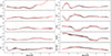 |
Fig. 3. Simulated (red) and observed SDSS DR16 (black; Ahumada et al. 2020) colors versus z. Data and filters are from SDSS-DR16 (ugriz, Lyke et al. 2020), UKIDSS-LAS (YJHK, Lawrence et al. 2012), and unWISE (W1W2, Schlafly et al. 2019). For each z bin, 200 combinations of parameters were drawn from the posterior, the thickness of the line denotes the ±1σ region of the simulated colors. |
As shown in Fig. 3, the average QSO colors are well represented, although some discrepancies are present for the J − H and H − K colors in the z ranges 0.8–1.2 and 1.2–1.6, respectively, which approximately correspond to the wavelength interval 6000 Å–1 μm. In this range, our predicted colors are bluer than the observed ones, likely due to a small residual host-galaxy contamination not accounted for in our modeling.
We finalized our SED templates by adding narrow emission lines to Type 2 AGNs, following the models by Feltre et al. (2016) and using the same approach and grid of parameters as in López-López et al. (2024). The narrow-line templates are then normalized according to the AGN LX − L[O III] relation from Lamastra et al. (2009). We applied extinction the templates, based on the host-galaxy optical depth provided by EGG, and using the reddening law by Calzetti et al. (2000).
Using our updated SED model, we then assigned an optical/UV SED to each AGN by drawing a set of best-fit parameters from the posterior distribution, and normalized the SED to the value of L2500 Å. We reddened the intrinsic SED by assuming an optical/UV extinction characterized by the AGN EB − V. We calibrated the distribution of EB − V to that suggested by SED fitting of Type 1 X-ray AGNs in the LSST Deep-Drilling Fields (DDFs; Zou et al. 2022). Instead, for Type 2 AGNs whose extinction arises from a (partially) obscuring torus, we used the observed EB − V distribution from Type 2 AGNs in XMM-COSMOS (Bongiorno et al. 2012). In both cases, we find the observed distribution well-represented by the functional form p(EB − V)∝[1+βn (EB − V)n]−1 (Hopkins et al. 2004; Krawczyk et al. 2015), with β = 15.20 and n = 1.58. For Type 2 AGNs, the data suggested an additional offset of +0.3 in terms of EB − V. We applied EB − V following the reddening law described in Temple et al. (2021). Examples of the final SEDs for Type 1 and Type 2 AGNs – including both the AGN and the host galaxy contributions – are shown in Fig. 4.
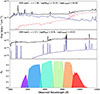 |
Fig. 4. Examples of AGN (blue) and galaxy (red) SEDs in the observer frame. The black line shows the combined SED. Top (middle): Luminous Type 1 (Type 2) AGN. Bottom: LSST ugrizy transmission curves. |
5. AGILE mock star catalog
Stars in the Milky Way and the Magellanic clouds are an important source of contamination to consider for the photometric selection of AGNs and quasars. For the stellar population in AGILE, we used “LSST SIM DR2” (Dal Tio et al. 2022), which is a simulation of the LSST stellar content down to r = 27.5 mag, including single and binary stars in the Milky Way and in the Magellanic clouds6.
These simulations are based on TRILEGAL (Girardi et al. 2005), a code for simulating the photometry of resolved stellar populations in any Galaxy field – as well as stellar systems such as clusters and galaxies – based on state-of-the art stellar evolution tracks (Bressan et al. 2012; Marigo et al. 2017; Pastorelli et al. 2019, 2020, and references therein). For each star, the simulation provides astrometry and photometry, parallax, and reddening, as well as physical and chemical properties, and proper motions. Additionally, pulsation periods are provided for variability modeling for stars in the Classical Cepheid (CC) instability strip or that are long-period variables (LPVs) in the asymptotic giant branch (see Sect. 7).
Dal Tio et al. (2022) provide two separate stellar catalogs, one for single stars (binary system fraction fbin = 0.0), and one limited to binary systems (fbin = 1.0), thereby allowing users to simulate any binary fraction by mixing the two catalogs. The binary star catalog itself is composed of the physical properties of the individual stars in the binary system, as well as the orbital parameters including the inclination to the observer. This allows for the simulation of binary eclipses. The provided binary star catalog only contains 10% of the expected binary systems. Therefore, following Dal Tio et al. (2022, Sect. 3.2) we adopted fbin = 0.40 by first downsampling the single star catalog to 60% and then adding in four times the binary stars in the same region.
For the purpose of our simulations, for each star, we used the equatorial coordinates, proper motions, and ugrizy photometry. Additionally, we made use of pulsation periods, when available, to simulate stellar variability, and for binary systems we further used the orbital parameters in order to accurately simulate binary eclipses. Both of these applications are described in Sect. 7.
6. The final AGILE mock truth catalog including AGNs, galaxies, and stars
We used the aforementioned recipes in order to build a single mock truth catalog of AGNs, galaxies and stars, on which we based the LSST image simulations as well as the photometric catalogs. This catalog spans a total area of 24 deg2, centered on the coordinates of the COSMOS field. We simulated the galaxy, AGN and stellar populations as described, assuming 0.2 < z < 5.5 (imposed by the COSMOS2020 SMF), and log10(Mstar/M⊙) > 8.5. We populated each galaxy with λSAR, labelled as AGNs the population with  , and derived the optical/UV properties for the AGN population. Finally, we added in the stellar population directly based on LSST SIM DR2, which is complete to r < 27.5 mag. The 24 deg2 truth catalog contains 164 005 CTN AGNs, 136 949 CTK AGNs, 7 147 592 non-active galaxies, and 624 637 stars, to a grand total of 8 073 183 objects.
6.1. Truth catalog contents
The final truth catalog considered here contains all the columns from the aforementioned processes for AGNs, galaxies, and stars. For AGNs, we include the physical properties such as LX, optical/UV luminosities, MBH, λSAR, Type 1 and Type 2 AGN classification, AGN EB − V, as well as the ugrizy absolute and apparent magnitudes derived from the AGN SED.
For galaxies (incl. AGN hosts), we include all the properties that are provided by EGG. This includes right ascension, declination, z, Mstar, SFR, passive or star-forming classification, morphological parameters (disk and bulge radii and luminosities), line attenuation (AV) for the galaxy bulge and disk, and ugrizy absolute and apparent magnitudes derived from the galaxy SEDs. For more details see the EGG documentation7 and Table E.1.
We note that the validation of the galaxy catalog and star catalog have already been performed in their respective works (Schreiber et al. 2017; Dal Tio et al. 2022). Here instead we focus the remaining validation part on the AGN catalog.
6.2. Validation of the AGN mock catalog
6.2.1. X-ray luminosity function
The first validation test performed on the mock truth catalog is to test the AGN X-ray luminosity function (XLF) against the literature values. In our approach, the AGN XLF is directly set by the combination of the SMF i.e., galaxy number density at a given Mstar, and p(λSAR | Mstar, z, T). The XLF thus provides an important test on the completeness of the underlying X-ray AGN population. To compute the XLF, we use the 24 deg2 truth catalog and calculate directly the resulting XLF at log10(LX/erg s−1) > 42 in several z bins. We show the results XLF in Fig. 5, and the comparison to the compilation of literature values (see Appendix A in Shen et al. 2020).
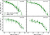 |
Fig. 5. X-ray luminosity function from the mock catalog compared to the literature. The panels correspond to different z values. The shaded region shows the XLF from the 24 deg2 mock catalog, while the green markers show the observed XLF compilation from various surveys (Shen et al. 2020). |
We find no apparent bias in the shape nor the normalization of the resulting XLF at z = 0.5–3.5, confirming that the X-ray AGN population is a complete sample of CTN AGNs. This is unsurprising, as Z24 have already shown that their p(λSAR) (regardless of quiescent or star-forming classification) combined with the Wright et al. (2018) SMF for all galaxies is consistent with the XLF of Ueda et al. (2014). Therefore, we effectively expand on their result by showing that a population of quiescent and star-forming galaxies from the COSMOS2020 SMF combined with their p(λSAR) for quiescent and star-forming galaxies are also in agreement with the XLF up to z = 4.
It is noteworthy that the recent discovery of “little red dots” poses a significant uncertainty for the luminosity function at z > 4 (e.g., Matthee et al. 2024; Ma et al. 2025). If their debated nature turns out to be of AGN origin, it would have a significant impact on our work at z > 4. However, in the context of LSST, the majority of the AGN population is still expected to reside at intermediate z ≲ 4, and detecting obscured AGNs in the first place from optical/NIR photometric data alone remains a challenge (Euclid Collaboration: Bisigello et al. 2025; Euclid Collaboration: Matamoro Zatarain et al. 2025). The modular nature of AGILE allows these populations to be included in future versions.
6.2.2. Optical number counts and luminosity function
The optical AGN and quasar populations arise in the truth catalog from the combination of X-ray and optical AGN properties. That is, the expected number of quasar-like optical AGNs is mainly driven by the XLF, LX–L2500 Å relation (Lusso et al. 2010), and the Type 2 AGN fraction (Merloni et al. 2014). We use the mock truth catalog to directly calculate both the expected sky number density of optical quasars, as well as the quasar luminosity function. We show the g-band number counts for the various classes of objects in Fig. 6, and the B-band quasar luminosity function in Fig. 7.
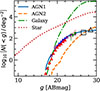 |
Fig. 6. Mock truth catalog (24 deg2) g-band number counts for Type 1 and Type 2 AGNs, galaxies, and stars. The colored markers show values from the literature (LSST Science Collaboration 2009, Fig. 10.7). The triangles correspond to Hartwick & Schade (1990, up), Beck-Winchatz & Anderson (2007, left and down), and Richards et al. (2006, right), while the squares correspond to Wolf et al. (2003). The open triangle shows the QSONumberCountMetric for the COSMOS DDF (see the text for the details), while the open square shows the expected QSO number counts for the ten-year LSST survey (Li et al. 2025a). |
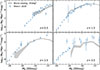 |
Fig. 7. B-band quasar luminosity function. The shaded regions show the luminosity function of mock Type 1 AGN from the 24 deg2 truth catalog. The markers show the recent data compilation of the quasar luminosity function from Shen et al. (2020) at the redshift indicated by the text. |
We find that the g-band number counts as computed from the 24 deg2 truth catalog are overall consistent with the literature (Richards et al. 2006; Wolf et al. 2003; Hartwick & Schade 1990; Beck-Winchatz & Anderson 2007) at g < 25. However, we find a slight overproduction of quasars at the bright end g < 18, likely ascribed to the choice of extrapolation of the Type 2 AGN fraction (see below). Moreover, within the 24 deg2 truth catalog, the errors in the number counts remain still relatively large, compared to the all-sky surveys from which the bright-end g < 18 observed number counts are measured from. At the expected LSST COSMOS ten-year depth, we also find the mock AGN number counts to be consistent with the expected LSST QSO number counts. Specifically, we refer to the DD:COSMOS CoaddM5 and DD:COSMOS QSONumberCountsMetric metrics calculated within the LSST Metrics Analysis Framework (MAF; Jones et al. 2014, and Sect. 8), and the expected QSO number counts from the ten-year LSST survey (black squares; Li et al. 2025a). Assuming the ten-year COSMOS DDF depth of g = 28.56, we find (530 + 754) deg−2 Type 1 and Type 2 AGNs in the mock. In the meanwhile, DD:COSMOS QSONumberCountMetric (baseline v4.0) suggests 637 deg−2, assuming a dithered COSMOS DDF area of ∼2 × 9.6 deg2. We note that here the g-band flux refers solely to the AGN flux, ignoring any host-galaxy contribution, which observationally would further complicate accurate measurements of the faint end of the number counts.
In addition, we measure the optical luminosity function of the mock Type 1 AGN population and compare it to the literature across a wide range in z ≈ 0.5–4.0 (Fig. 7). We note that the luminosity function was computed using the AGN intrinsic absolute magnitude that was de-reddened according to the EB − V. We find that both the shape and the normalization of the B-band quasar luminosity function are in general agreement with the observed one (Shen et al. 2020). At higher z ≈ 3.5 the mock under-predicts the luminosity function at the ∼0.2–0.4 dex level in the MB > −25 regime. As anticipated, these discrepancies could be mitigated by fine-tuning the extrapolation strategy of the Type 2 AGN fraction (Merloni et al. 2014), especially at z ∼ 0.5 and z > 3. Moreover, the low-luminosity tail of the z ∼ 3.5 luminosity function suffers from more uncertain comparison data. Given these, we refrain from further optimizing the extrapolation of the Type 2 AGN fraction.
6.2.3. Active black hole mass function
The active black hole mass function (BHMF) is an important observable validating the assignment of AGNs to galaxies. It is the by-product of three key components in the mock truth catalogs, i.e., the galaxy SMF (Weaver et al. 2023), the MBH–Mstar relation (e.g., Zou et al. 2024a, and Sect. 4.2), and the probability of a black hole being active (e.g., Z24). In order to further validate the mock truth catalog, we compare the predicted active BHMF from the 24 deg2 mock catalog to the observed local (0.21 ≤ z < 0.30) active BHMF of Ananna et al. (2022). Their analysis is based on a complete z < 0.3 sample of ultra-hard selected (14–195 keV) X-ray AGNs from the Swift-BAT AGN Spectroscopic Survey (BASS; Koss et al. 2017, 2022), which is more sensitive toward CTK AGNs compared to the typical 2–10 keV band selection. Thus, we calculate the active BHMF including both CTN and CTK AGNs, and Eddington ratio λEdd limits as in Ananna et al. (2022). To be consistent with the assumptions in the continuity equation (Sect. 4.2), we converted mock MBH and LX to λEdd assuming a constant bolometric correction kbol = 25. As shown in Fig. 8, the mock truth catalog successfully reproduces the normalization and general shape of the local active BHMF.
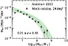 |
Fig. 8. Local active BHMF. Both the mock truth catalog (symbols) and observed (lines and shaded region; Ananna et al. 2022) active black hole mass functions correspond to Eddington ratios −3 < log10λ < 1. The mock λ is estimated from MBH and LX, assuming a constant bolometric correction LX / Lbol = 25. |
The comparison with higher-z BHMF measurements is less conclusive, as the mock BHMF is systematically below the best-fit model by, for example, Schulze et al. (2015). This is unsurprising given the large uncertainties in the MBH–Mstar relation at high z. While the continuity equation adopted here predicts a nearly z-invariant MBH–Mstar relation consistent with the local relation (Reines & Volonteri 2015), observational constraints at higher-z remain highly uncertain and span a wide range of normalizations (e.g., Merloni et al. 2010; Suh et al. 2020; Pacucci et al. 2023; Maiolino et al. 2024; Tanaka et al. 2025).
7. Optical variability
The mock catalog created thus far depicts a purely static universe. However, the strength of LSST lies in its high cadence, where a sky position will be imaged on average once every three nights (see Sect. 8). Here we describe the recipes to add in optical variability into the simulation for different classes of objects. We first included a model for AGN variability, and second we considered stellar variability for CCs, LPVs, and binary star systems. We did not consider transient phenomena such as supernovae, or tidal disruption events.
7.1. AGN variability
Active galactic nuclei exhibit stochastic variability at all wavelengths and with timescales ranging from minutes to years (Paolillo & Papadakis 2025). Continuum optical light curves have been empirically described as a damped random walk (DRW; Kelly et al. 2009), a first-order continuous autoregressive moving-average (CARMA) process modeling variability with two main parameters: the amplitude of correlation decay σ, and a characteristic damping timescale τ. In detail, variability is described with an exponential decay autocorrelation function (ACF), where the covariance between two points separated by Δt is given by a combination of Gaussian processes as
 (5)
(5)
The DRW predicts a power-law power spectral density for AGNs, with a spectral index of −2, flattening to zero for ≫τ. Such a model has been successful in describing both the stochastic and the typical red-noise trend of AGN light curves with lengths of the order of a few years, although deviations have been observed on both longer and shorter timescales with possibly steeper high-frequency slopes and longer decorrelation timescales for a complete flattening (e.g., Mushotzky et al. 2011; Guo et al. 2017; Arévalo et al. 2024). Albeit more refined methods have been proposed, such as fitting light curves with higher-order CARMA processes (e.g., the damped harmonic oscillator, Yu et al. 2022), direct or indirect estimation of the power spectral density (e.g., Kelly et al. 2014; Petrecca et al. 2024), or unsupervised machine learning analysis of time series (Tachibana et al. 2020), there is still no definitive model to describe AGN optical variability.
While it might not be the most accurate description on short (less than a few days) or very long (more than a few years) timescales, the DRW provides a robust and well-tested first-order approximation and comes with a flexible and easy way to produce simulated light curves (Suberlak et al. 2021). Thus it provides a controlled baseline model with which the other aforementioned models may be compared to. Moreover, it has a direct connection with the structure function (SF), which is typically used to parametrize AGN light curves in the temporal domain instead of the power spectrum. The SF is defined as the root mean square magnitude difference as a function of the time difference Δt between observation pairs (Kozłowski 2016), and it is related to the ACF (and thus the DRW) as ![Mathematical equation: $ \mathrm{SF}(\Delta t) = \sqrt{2\,\sigma^2 \left[ 1 - \mathrm{ACF}(\Delta t) \right]} = \mathrm{SF}_\infty \sqrt{1 - \exp \left(-|\Delta t| \,/\, \tau \right)} $](/articles/aa/full_html/2026/06/aa58627-25/aa58627-25-eq7.gif) . Here, we used the ACF of the DRW from Eq. (5), and introduced
. Here, we used the ACF of the DRW from Eq. (5), and introduced  as the variability amplitude for Δt → ∞, typically used as a parameter in ACF analyses together with τ.
Both DRW and the associated SF parameters have been observed to correlate with physical AGN properties, such as MBH, accretion rate, bolometric luminosity and rest-frame wavelength (e.g., MacLeod et al. 2010; Zu et al. 2013; Kasliwal et al. 2015; Suberlak et al. 2021). In particular, we used the latest DRW parameters calibrated using the 15 yr baseline for 9248 quasars selected from the SDSS Stripe-82 and crossmatched with Pan-STARRS1 (Suberlak et al. 2021, references therein, and Table 1 of Paolillo & Papadakis 2025) in order to assign each AGN in the simulation a ten-year DRW light curve. The parameters τ and SF∞ scale with the physical AGN properties via
 (6)
(6)
where f is used to denote either τ or SF∞, and both parameters have their separate best-fit values A, B, C, and D as summarized in Suberlak et al. (2021, Table 2). Here λRF and Mi correspond to the rest-frame wavelength (set by the LSST band and z) and the absolute magnitude in the i-band, respectively. Light curves were simulated using the DRW implementation by Kovačević et al. (2021), and providing the SF∞ and τ parameters derived from the scaling relations as input.
The scaling relations to calibrate the DRW parameters used for this simulation were derived from a sample of quasar-like AGNs with a certain range of masses and bolometric luminosities. Although this is quite large, with log10(MBH/M⊙) ≈ 7.0–10.5 and log10(Lbol/erg s−1) ≈ 44.5–47.5, it does not cover the full variety of simulated AGNs. Whenever we had to simulate a DRW for a source outside the range of SDSS Stripe-82 quasars, we extrapolated the scaling relations and confirmed that the recovered light curves had variability amplitudes compatible to those reported in literature.
Another important consideration is related to Type 2 AGNs, which are typically missed by optical surveys because of the high degree of obscuration. For this reason, large statistical studies of variability usually focus on non-obscured sources. However, this is expected to change with LSST where subtracting the host-galaxy contribution via difference image analysis (DIA) on the entire dataset with an extended temporal baseline is possible. Many recent works report Type 2 AGNs to feature suppressed variability with a flatter SF (e.g., De Cicco et al. 2022; López-Navas et al. 2023). To simulate Type 2 AGN light curves compatible with these observations, we used the same scaling relations as for Type 1, but adding an over-damping factor of ten to both SF∞ and τ (López-Navas et al. 2023). Although this empirical factor introduces some uncertainty, it is worth stressing that the main aim of this simulation is to test the capability of LSST to recover the input, focusing on any bias due to the observing strategy, the photometry, or the reduction pipeline.
Here we have only focused on the average red-noise variability of the typical AGNs. For example, our AGN variability model does not consider the time lag between the bands, but there are specific works studying this in the context of LSST (e.g., Czerny et al. 2023). Also, other relatively rare sources such as blazars, binary AGNs, or extreme variability phenomena (e.g., changing-look AGNs, outbursts, and deep fades; see Komossa et al. 2026 for a recent review) are not included.
7.2. Star variability
Using the orbital parameters from the binary star catalog (Sect. 5), it is straightforward to simulate the light curves of eclipsing binaries in the LSST ugrizy filters. Toward this goal, we have used the batman software (Kreidberg 2015). Further stellar variability relevant for this study comes from stellar pulsation. In its current version, the TRILEGAL simulation includes only two types of pulsating stars, namely CCs and LPVs, for which pulsation periods are provided. Other variability parameters for these stars (amplitudes, light curves), as well as additional pulsating star types are planned for future versions of the simulation (Dal Tio et al. 2022). Considering the scope of the present work and the effort that would be required to add information for other variability types, we preferred to limit our study to the most common variability manifestations that have already been validated in the simulations. For these, we adopted the following procedures in order to simulate light curves.
7.2.1. Classical Cepheids
The CC pulsation models used to generate the theoretical light curves in the LSST filters were derived from a nonlinear, convective hydrodynamical approach, specifically employing the Stellingwerf hydrodynamical code (Bono et al. 2000a,b). This dataset extends previous pulsation models (e.g., Caputo et al. 2000; Fiorentino et al. 2007, and references therein) by including, simultaneously, variations in chemical composition, mass-luminosity (M–L) relation, and superadiabatic convection efficiency. The models are computed for fundamental (F), first overtone (FO), and second overtone (SO) pulsation modes, considering four different chemical compositions: Low-metallicity cases: Z = 0.004, Y = 0.25 and Z = 0.008, Y = 0.25, Solar-like metallicity: Z = 0.02, Y = 0.28 and supersolar metallicity: Z = 0.03, Y = 0.28. The models cover a wide range of stellar parameters, including effective temperature: 3600 K to 7200 K, in steps of 100 K and mass range from 3 to 11 M⊙, in steps of 1 M⊙. The convective efficiency is parameterized using the mixing length parameter αml = 1.5 (standard convective efficiency, αml = 1.7 and αml = 1.9).
Moreover, three M–L relations are adopted, following the formulation provided by Bono et al. (2000a): case A i.e., canonical models with no core overshooting, rotation, or mass loss, case B i.e., non-canonical models with a moderate luminosity increase of Δlog10(L / L⊙) = 0.2 dex and case C i.e., non-canonical models with a stronger luminosity increase of Δlog10(L / L⊙) = 0.4 dex. For this study, we selected models that satisfy the luminosity range adopted in the simulation (2.5 < log10(L / L⊙) < 4.8). Specifically, we selected
-
fundamental and first overtone mode models,
-
all four chemical compositions,
-
αml = 1.5 and
-
non-canonical M–L relation (case B, over-luminous by 0.2 dex).
For a comprehensive description of the assumptions underlying the CC pulsation models and the key results such as the topology of the instability strip, the period–luminosity–color (PLC) relations, and LSST light curves adopted for this work, we refer the reader to De Somma et al. (2020, 2022, 2024).
7.2.2. Long-period variables
Long-period variable stars represent the final stages in the evolution of low- to intermediate-mass stars (0.8 ≲ Minit / M⊙ ≲ 8). They are cool, red giant stars with peak emission in the red or NIR, and display photometric variability with periods of order of several days to a few years, often with cycle-to-cycle variations and various degrees of regularity. Depending on the spectral range of observation and intrinsic stellar properties, they span a range of photometric amplitudes, from a milli-magnitude level up to more than ten magnitudes in the visual filters.
The TRILEGAL simulation of the LSST stellar content includes pulsation periods of LPVs based on stellar pulsation models of Trabucchi et al. (2019, 2021), as well as an indication of the dominant pulsation period. Synthetic light curves of LPVs, and their photometric amplitudes, are not currently available in TRILEGAL simulations. To the best of our knowledge, no prescription is available from the modern scientific literature to predict these features as a function of global stellar parameters. Therefore, we relied on a simplified, semi-empirical description.
We took advantage of the fact that LPVs follow a period-amplitude relation (e.g., Trabucchi et al. 2019, and references therein). We examined the I-band photometric time series of LPVs in the Magellanic Clouds observed as part of the Optical Gravitational Lensing Experiment (OGLE; Soszyński et al. 2009, 2011), and derived an approximate analytic relation
 (7)
(7)
where P1 is the primary variability period and σI is the standard deviation of the I-band light curve, which is a tracer of the variability amplitude. To convert it into the LSST ugrizy filters we adopted the results of Iwanek et al. (2021). Finally, we assumed that the light curve can be modeled as a simple sine with randomized phase offset.
This approach to model the photometric variability of LPVs is rather crude: the period-age relation suffers from a relatively large scatter, and both the regularity of the light curve and the relation between peak-to-peak amplitude and the standard deviation depend on the degree of multi-periodicity of a star. Nonetheless, it provides us with an efficient method of estimating the order-of-magnitude impact of LPVs as a source of confusion against AGN variability, which is an acceptable trade-off for the purpose of the present paper.
8. Image simulations
The detailed LSST ten-year survey plan is defined in the baseline strategy (see Ivezić et al. 2019; Bianco et al. 2022, and references therein). Overall, the majority of the survey time is expected to be dedicated to the Wide Fast Deep (WFD), which covers the southern sky, while some 7% of survey time is dedicated to the DDFs. The DDFs are five extragalactic fields covered by one to two telescope pointings and to several magnitudes deeper compared to the WFD8. Notably, the COSMOS DDF is the deepest of the planned DDFs, and receives approximately twice the number of visits compared to any other DDF. On the contrary, the Euclid Deep Field South visits are split between two LSST pointings.
The LSST survey strategy is described as a sequence of visits, each corresponding to a single telescope pointing, a chosen filter (ugrizy), and the exposure time (nominally tgrizy ∼ 29.2 s, and tu = 38 s). Within LSST, survey strategies are evaluated and simulated using the Operations Simulator9 (OpSim), and the Metrics Analysis Framework (MAF; Jones et al. 2014). In addition to the telescope information, these simulations also provide the expected local sky conditions such as the positions of the Sun and the Moon, air mass, and seeing. Here we adopted the latest survey strategy (at the time of initiating this work), “baseline v4.0” as the reference. Differences between various survey strategies are detailed on-line10. We focused on the COSMOS DDF, which is one of the most well-known regions of the extragalactic sky in terms of depth and wavelength coverage (see Weaver et al. 2022).
According to baseline v4.0, the ten-year LSST survey contains a total of 2 038 634 visits, with 43 594 in the COSMOS DDF. The total number of COSMOS visits per LSST ugrizy band are 2185, 5033, 9919, 9994, 11 538, 4925, respectively. Temporally, the first half of the visit is completed within the first three years of the survey. In the DDFs, visits are further grouped into “sequences” so that every time a DDF is observed, multiple exposures are taken in succession instead of a single one (Nugrizy = 8, 10, 20, 20, 24, 18). In contrast, in baseline v5.0 (the latest strategy at the time of writing) the “ocean” DDF strategy is adopted. Here, DDF sequences would alternate between shallow (fewer visits per sequence) and deep (more visits per sequence) seasons. The most of the DDF visits would then occur in the deep seasons, of which there is at least one per DDF. These OpSim runs are available on-line11.
8.1. The instance catalogs
The LSST cadence is used by AGILE – together with the original mock catalog and light curve information – to generate the so-called instance catalogs. These catalogs correspond to a snapshot of the mock catalog at the time of each LSST visit. The instance catalogs describe the position (varying for stars based on their proper motions), apparent magnitude (varying for stars and AGNs based on their light curves), and the morphology of each object. Following Schreiber et al. (2017, Sect. 3.2), we described galaxies as a combination of two Sérsic profiles assuming n = 4 for the bulge and n = 1 for the disk. For AGNs, an additional point-like component was added on top of the galaxy bulge and disk at the center, while stars were considered to be point-like sources.
8.2. Raw simulated LSST images
The synthetic LSST raw images are generated by AGILE from the instance catalogs using DESC software called IMSIM12. This software simulates the 3.2 Gigapixel LSSTCam instrument accurately13, including electronic (e.g., bias, dark current, and non-uniformity) and atmospheric effects (e.g., seeing). The LSSTCam is a large mosaic camera, composed of a total of 189 individual detectors, which fully cover the 9.6 deg2 field of view (FOV) of the telescope. With IMSIM, any subset of the 189 detectors may be simulated individually, resulting into realistic synthetic LSST raw exposures.
8.3. Final simulated science images
Raw LSSTCam exposures were then converted into calibrated single-visit exposures called calexp14 images by first removing the signal of the instrument and performing the calibration in both astrometry and photometry. For astrometric and photometric calibration, the mock truth catalog was used as the reference catalog, including proper motions for stars. We did not consider photometric nor astrometric errors arising from the reference catalog, which is an additional source of error in the actual LSST data. As per the LSST requirements, the expected calexp depths in the ugrizy bands are 23.9, 25.0, 24.7, 24.0, 23.3, and 22.1 (5σ), respectively (Bianco et al. 2022). However, individual calexp image depths will depend on the survey cadence and will be further modified by air mass, seeing, and the final survey strategy.
Finally, the individual single-visit calexp images were combined to create deep coadded images in each of the LSST ugrizy bands. In the coaddition, the sky was first tessellated into tracts, which are defined as partially overlapping rectangular regions with a side length of 1.6 deg. Each tract is divided further into 7 × 7 patches, while each patch is further subdivided into 4100 × 4100 pixels with a pixel scale of  . In each pixel, the coadded value is the result of resampling and combining the corresponding single-visit calexp images. In the LSST requirements, the expected ten-year coadded image depths in ugrizy are 26.1, 27.4, 27.5, 26.8, 26.1, and 24.9 (5σ), respectively (Bianco et al. 2022).
Figure 9 shows an example zoom-in of calexp and coadded images in the r-band. The coadded image includes a total of 289 visits in the COSMOS field based on the baseline v4.0 and the 24 deg2 truth catalog, highlighting the increase in depth incrementally as the survey progresses. In addition, Fig. 9 shows the positions of individual truth catalog AGNs, galaxies, and stars.
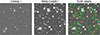 |
Fig. 9. Example single-visit (calexp; left), deep coadd (middle) images, and the underlying truth catalog labels (right). The images correspond to the r-band with a small field of view of 2′ centered around |




For these tasks of reduction, calibration, and coaddition, AGILE uses the LSST Science pipelines (v8.0.0, w_2024_16; Bosch et al. 2018), For more details, also refer to Dark Energy Science Collaboration (2021).
9. Photometric catalogs
The last step of AGILE is to perform the photometric analysis of the single-visit and coadded images. This was done using the LSST Science pipelines (v8.0.0, w_2024_16). Starting with the deep coadded images, AGILE performs source detection at a significance level of S/N > 5 in order to create the object table. For each detection, the object table contains the set of ugrizy positions and flux measurements, the characterization of the morphology of the source, and quality flags. AGILE also performs forced photometry at the coordinates of each object in each single-visit calexp image. This results in a forced photometry catalog, where each object has their corresponding measured ugrizy light curve in accordance with the input LSST baseline. These data products are detailed in the Rubin-LSST documentation to which we provide the relevant links in Table E.
Some of the Rubin Data Products have different scientific applications compared to ours, such as measurements from the DIA. Having the focus on the AGN population, we proceed on with the discussion of the photometry within the object catalogs from the deep coadded images, as well as the forced photometry catalogs from the single-visit images.
Throughout the following sections, we base the analysis on the AGILE DR1 photometric catalog corresponding to 1 deg2 (21 out of 189 LSSTCam detectors) and 1441 visits over three years of observations in the COSMOS DDF. The catalog and the assumed detector layout are described further in Appendix D.
9.1. Object catalogs
The object catalog is constructed by measuring the properties of extracted sources (S/N > 5) from the coadded ugrizy images. Each object defined this way contains a total of 1186 columns of information consisting of astrometric (e.g., RA, Dec, and their respective errors), morphological (e.g., Kron radii and extendedness), and photometric (e.g., ugrizy flux measurements) measurements. The fluxes and their errors are provided for a wealth of definitions, including aperture, point-spread function (PSF), and composite model or cModel. The fluxes and their quality flags are also reported for each band separately.
As an example of the source density, we use the object catalog produced from the 1441 visits in COSMOS. We select a single patch, which corresponds approximately to the area of one LSSTCam detector ∼0.05 deg2 with a total of 12 082 objects. Out of these, 9171 have S/N > 5 (psfFlux) in the r-band, and a further 1985 have also r < 24, giving an approximate source density of 0.19 M deg−2 with S/N > 5, and 40 K deg−2 with S/N > 5 and r < 24. These densities may be directly compared to the underlying truth catalog, where the 24 deg2 truth catalog suggests total (AGN, galaxy, or star) source densities of 50 K deg−2 (40 K deg−2) at r < 24 (r < 23.7). The apparent discrepancy arises from a combination of deblending losses and underestimated galaxy true fluxes by the psfFlux. Indeed, by computing the number of close angular pairs in the truth catalog in a similarly sized area and assuming r < 24, we find a significant incompleteness in terms of angular pairs at < 2″ (close to 100% at < 1″). However, this accounts only for a few hundred missing pairs overall and therefore cannot explain the full discrepancy. At larger separation, the discrepancy is instead consistent with underestimated galaxy fluxes by psfFlux. Repeating the density calculation with cModelFlux yields a source density of 51 K deg−2, supporting this idea. This is examined in more detail in the next section.
9.2. Photometric accuracy
We evaluated the photometric accuracy across different classes of objects and different flux definitions, notably the psfFlux, the calibFlux (12 pixel aperture flux), and the cModelFlux. We matched the objects with their truth catalog counterparts by minimizing the combined difference in both measured position and flux. To quantify the accuracy of the r-band flux, Fr, we calculated both the normalized median absolute deviation (NMAD) σNMAD ≡ 1.48 × |Fr − Fr, truth| / Fr, truth as well as the catastrophic outlier fraction η (i.e., fraction of objects with |Fr − Fr, truth| / Fr, truth > 0.15). Given that the measured flux uncertainties naturally increase toward fainter fluxes, we calculated these statistics in three separate bins from rtruth = 20 to rtruth = 26. We summarize all our results in Fig. 10 and Table F.1. Here we focus on the 20 < r < 22 results in order to highlight the systematic differences between the populations.
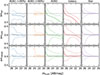 |
Fig. 10. Accuracy of the LSST Science Pipelines flux estimators for different classes of objects. Each panel shows the median (10th and 90th percentile) magnitude difference between the measured flux and the truth flux in the r-band. Rows correspond to the flux estimated using psfFlux, calibFlux (defined as the 12 pixel aperture flux), and cModelFlux, respectively. Columns correspond to the truth labels, as shown at the top of each column. |
We start by discussing the stellar and galaxy populations. As expected, we find stars best described by their measured psfFlux, with the lowest σNMAD = 0.003, across the different flux definitions. In addition, we find η = 0.001 for all flux estimates. On the contrary, we find galaxies best described by their cModelFlux at σNMAD = 0.07 (cModelFlux) compared to e.g., σNMAD = 0.108 (calibFlux). Especially for bright galaxies, the aperture fluxes tend to bias low due to the unaccounted for extendedness of the source. Indeed, we observe the two estimates to agree better toward fainter fluxes (see Fig. 10).
Type 1 AGNs and their hosts form complicated morphologies from pointlike-QSOs to galaxy-dominated systems with centrally concentrated AGN emission. To account for this, we measured separately the accuracy for systems that are AGN-dominated (host-contaminated), based on whether the AGN flux accounts for > 90% (< 90%) of the total flux. We find that apart from psfFlux for host-contaminated systems, all flux estimates recover the true flux on average without the biases present as for bright galaxies. The effect of the host-galaxy contamination is clearly detected in the measured AGN psfFlux (top-left panel of Fig. 10), and in the high outlier fraction (η = 0.477; see Table F.1). We find the results for Type 2 AGNs, similar to the galaxy ones as is expected from AGN obscuration.
Finally, in Table F.1 we report on the flux accuracy on sources split by morphology, defined as the extendedness as measured in the r-band. Overall our findings remain unchanged. That is, pointlike sources are best described by either their psfFlux (σNMAD = 0.071) or cModelFlux (σNMAD = 0.108). For extended sources, we find cModelFlux to perform the best (σNMAD = 0.071), followed by calibFlux (σNMAD = 0.108). As expected, the use of psfFlux results in highly biased estimates with η = 0.546.
These results highlight that at level of the flux definition, no single flux definition fully and accurately captures the diverse AGN population. Our results indicate that, overall, the cModelFlux has the least amount of problematic cases, while psfFlux is clearly preferred for point-like sources. For AGN population studies, a strategy utilizing a combination of fluxes based on measured extendedness is preferred.
9.3. Forced photometry, limiting magnitude, and extracted light curves
We explore the accuracy of forced photometry catalog, based on forced photometry as performed on the positions of the objects detected in the deep coadded images. The forced photometry extraction was performed on each single-visit image individually. We measured the photometric accuracy using psfFlux and psfFluxErr from the forced photometry catalog, and limiting the analysis to pointlike sources. We estimated the 5σ depth (m5) as the magnitude at which S/N = 5. For the ugrizy bands using forced photometry, we find  ,
,  ,
,  ,
,  ,
,  ,
,  (errors correspond to the 16th and 84th percentiles).
This is in overall good agreement with the LSST error estimates as forecast in Ivezić et al. (2019). They provide an analytic formula to compute m5, which depends on the band, air mass, seeing, and sky background (Ivezić et al. 2019, Eq. 6). To facilitate for an accurate comparison between their work, we re-estimated their m5 with the median air mass, seeing, and sky background using the LSST baseline v4.0 in COSMOS. We find m5 = (23.32, 24.25, 23.89, 23.41, 22.83, 21.93) (ugrizy), which is within the errors of Ivezić et al. (2019), but systematically brighter by 0.1–0.3 mag. Although part of this discrepancy can be attributed to Galactic extinction, this effect is expected to be very small, if not negligible, in a field such as COSMOS. Moreover, the relatively large errors – mostly attributed to variations in the air mass – highlight the need to exercise care when condensing the limiting magnitudes to a single number.
As an example of the photometric accuracy using forced photometry, we show the ugrizy light curve of the brightest QSO in the simulation in Fig. 11. Moreover, in the same figure, we also show the r-band light curves of four bright AGNs from the simulation.
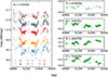 |
Fig. 11. Left: example light curves in the LSST bands of bright AGNs within AGILE DR1. The markers show psfFlux AGN light curves from the forced photometry catalogs, while the lines correspond to the truth catalog light curves in the same bands (indicated by the colors). As explained in the text and Appendix D, only the first exposure of each DDF sequence is shown, and the measured light curves span the first three years of simulated LSST operations in the COSMOS DDF according to baseline v4.0. Right panels: light curves only in the r-band of four bright AGNs. Otherwise, the axes and the units are the same as in the left panel. Top right: AGN (ID = 6289499) located close to the edge (< 1″) of the detector layout (Fig. D.1). It is sampled less frequently compared to the rest. |
10. AGN science applications
In this section we move beyond using the photometric catalog solely for testing technical aspects of the LSST pipeline and explore its potential for scientific applications in the context of AGN science. In particular, here we present the results we obtained by applying classical Type 1 AGN selection techniques based on color and variability.
In real LSST observations, source classification will leverage the full range of available data, likely through machine learning (ML) approaches (e.g., Savić et al. 2023). However, this is not the goal of this section, and the development of advanced techniques for identifying AGNs using the AGILE catalogs is deferred to future work. This analysis provides an opportunity to further validate the catalog by applying well-established AGN selection techniques that are effective at identifying bright, QSO-like Type 1 AGNs. Moreover, it allows for the quantification of the completeness and purity of these methods using an intrinsically complete and well-characterized mock sample.
10.1. AGN color-color selection
Color-color diagrams have been widely used to identify Type 1 AGNs since their discovery (e.g., Schmidt & Green 1983; Richards et al. 2002; Croom et al. 2009; Euclid Collaboration: Matamoro Zatarain et al. 2025), as these sources occupy a distinct locus in the multidimensional color space that separates them from inactive galaxies and main-sequence stars. Early selection methods relied on morphology and simple U − B color cuts to identify sources with an UV excess, due to the blue bump of the accretion disk (e.g., Sandage et al. 1965; Schmidt 1963). Over time, the increasing availability of multi-band photometry and a refined understanding of the AGN locus have led to more sophisticated color-based selection criteria (e.g., Fan et al. 1999; Richards et al. 2002; Croom et al. 2009), significantly improving the efficiency and completeness of AGN identification.
Toward this end, we first selected objects from the photometric catalog based on the three-year coadded images. For these objects, we then applied the selection criteria proposed by Croom et al. (2009, Eqs. (1)–(3)) to identify QSOs in the 2SLAQ survey at z < 2.6. Since the criteria by Croom et al. (2009) are designed to select luminous QSOs, they include relatively strict cuts in observed flux, limiting the selection to bright sources with g < 21.85 and i < 22. These constraints significantly narrow the AGILE DR1 sample: 120 Type 1 AGNs (out of 685 detected in the object table), 37 Type 2 AGNs (out of 9487), 1186 galaxies (out of 253 243), and 3184 stars (out of 27 345) satisfy the selection. In Fig. 12 we show the color-color diagrams for these sources. Following Croom et al. (2009), we use PSF magnitudes.
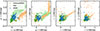 |
Fig. 12. Observed color-color diagrams using the LSST bands for detected AGILE sources. The markers and colors correspond to the labels of galaxies (or Type 2 AGNs), stars, and Type 1 AGNs in accordance with the legend, and corresponding to the true labels. A darker color is used to mark sources selected using the Croom et al. (2009) criteria. Only bright sources, g < 21.85 and i < 22, are shown. |
Among the 120 bright Type 1 AGNs, 116 lie at z < 2.6, of which 77 are correctly identified using the Croom et al. (2009) selection criteria. However, the same criteria incorrectly classify 48 stars, 140 galaxies, and eight Type 2 AGNs as Type 1. Restricting the sample to sources with g < 21.85 and i < 22, the Croom et al. (2009) criteria yield a completeness of 65% (67% when considering only z < 2.6) but a high contamination rate of 72%.
To compare with Croom et al. (2009), we split our sample into two g-band magnitude bins. For g ≤ 20.5, we recover 30 out of 31 AGNs, consistent with the ∼100% recovery reported for very bright sources, although the contamination remains high at 63%. For 20.5 < g < 22, we correctly identify 47 / 84 Type 1 AGNs, corresponding to a slightly lower completeness than the ∼70% reported by Croom et al. (2009) for the same range, with a contamination of 75%.
Following Croom et al. (2009), we did not apply any morphological selection. However, introducing the additional requirement for the sources to be point-like in their reference band (refExtendedness = 0) reduced the number of Type 1 AGNs that satisfied all conditions down to 57 (45 of which are correctly selected). This effectively removes all galaxy and Type 2 AGN contaminants, dropping the contamination to 43%.
10.2. Variability analysis
The AGN optical continuum variability is a key feature for their discovery as it has proven to be an effective method for distinguishing Type 1 AGNs from other types of sources (e.g., van den Bergh et al. 1973; Koo et al. 1986; Sánchez-Sáez et al. 2019; De Cicco et al. 2021; Savić et al. 2023; Paolillo & Papadakis 2025). Here, we present a simple test to quantify the LSST AGN recovery performance based solely on the variability of the sources. Nowadays, AGN selection via variability relies on computing a large set of features from the light curves (e.g., Savić et al. 2023; De Cicco et al. 2025); however, for simplicity, we adopt a single low-statistics variability metric, the root-mean-square (RMS) deviation (e.g., Sesar et al. 2007; Trevese et al. 2008; Sarajedini et al. 2011; Pouliasis et al. 2019).
For extended sources, PSF fluxes exhibit artificial variability due to variations in the PSF, atmospheric conditions and positional inaccuracies. Due to this, for this analysis we used psfFlux + psfDiffFlux, where psfFlux is the (constant) flux from the coadded template image, and psfDiffFlux is the difference flux compared to the template image. For AGNs, this accounts for both the seeing, and the host galaxy (depending on the deblending quality), while for galaxies and stars this expression reduces on average to psfFlux. We restricted the analysis to sources detected in the r-band in at least ten separate epochs, with detections defined by a signal-to-noise ratio of S/N > 5. We also required sources to have no failures in their psfFlux and extendedness measurements (i.e., r_psfFlux_flag = r_extendedness_flag = 0 in the object table). Finally, to minimize photometric issues, we excluded sources located near the survey edges and in the proximity of bright, saturated, stars (e.g., Poulain et al. 2020). Specifically, we excluded an annular region within 2′ of the survey boundary and masked objects within 2′ of stars with r < 9 and within 1′ of stars with r < 11.5. These final cuts reduced the final analyzed sample by ∼10%.
The RMS can be strongly affected by photometric outliers. To account for this, we clipped the light curves by excluding points more than 5σ away from the median magnitude. We investigated this outlier fraction in terms of relevant simulation parameters. We found that a single exposure has an elevated outlier fraction mainly due to a low number of PSF stars (NPSF). We used r < 24, point-like, and non-flagged detections with N > 30 observations to quantify the outlier fraction. We found that a typical exposure (NPSF = 124) has an outlier fraction of 0.4%. At a low percentile (NPSF < 40 or 1%), this fraction elevates steeply to 10% and above. Moreover, we find that NPSF and seeing θ are strongly anti-correlated (R = −0.95). We find θ < 2″ to yield securely NPSF > 40, while NPSF = 124 corresponds to  . These findings have important implications for LSST observations, and care should be taken in using seemingly good-quality (i.e., non-flagged) observations for variability analyses.
In Fig. 13 we show the RMS as a function of psfFlux magnitude. A clear trend is visible: fainter sources exhibit higher RMS values due to the increasing relative contribution of background noise, while at bright (r < 18) magnitudes the RMS flattens at ∼0.005 mag, consistent with the typical level of systematic uncertainty. Assuming that the vast majority of sources are non-variable, we computed the median observational RMS and its median absolute deviation (MAD)15 in bins of magnitude. Following Pouliasis et al. (2019), we selected as variable those sources with an RMS exceeding the median by more than three times their MAD. We adopted the lower threshold of three (rather than three and a half) because the much higher number of epochs in our dataset makes the RMS converge more reliably to the true, magnitude dependent, value (e.g., Trevese et al. 2008). We performed this method separately for extended and point-like sources (e.g., Sarajedini et al. 2011; Pouliasis et al. 2019). All sources with r < 16 were treated as non-variable since their variability measurements are affected by saturation.
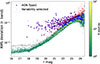 |
Fig. 13. Magnitude versus RMS deviation in the r-band. Sources that are more than three times the MAD above the median of the distribution in a magnitude bin were selected as variable and labeled with red markers. Blue squares indicate Type 1 AGNs. The solid and dotted black lines represent the thresholds used to select variable sources for point-like and extended sources, respectively. |
The recall power of this selection method depends strongly on source magnitude. Overall, we recovered 53% of Type 1 AGNs present in the catalog after applying the quality cuts (225 / 421). However, the recovery fraction varies significantly with brightness: 98% (64 / 65) for sources with r ≤ 21, 91% (68 / 75) for 21 < r ≤ 22 and only 33% (93 / 281) for r > 22, where the typical AGN variability amplitudes become comparable to the observational scatter. Compared to Trevese et al. (2008), who reported a completeness of 44% for V < 24 sources, based on an eight-epoch survey with the Wide Field Imager, we find a higher recall. Restricting our analysis to the same magnitude range (though in a different band), we obtain an overall completeness of 61% (223 / 366). This improvement is not surprising given the higher signal-to-noise ratio at the adopted magnitude limit and the higher LSST sampling rate.
We also investigated the dependence of completeness on physical parameters, finding that the selection preferentially identifies systems hosting more massive black holes and/or accreting at higher Eddington ratios. This trend primarily reflects the imposed magnitude limit, rather than the variability prescription described in Sec. 7.1. Within a fixed redshift bin, a detectability cut such as r < 22 effectively corresponds to a luminosity threshold, which translates into a bias toward higher black hole masses and/or higher Eddington ratios. Although the adopted variability prescription assigns greater intrinsic amplitudes to BHs with a lower mass and less luminous AGNs, this effect is subdominant compared to the bias introduced by the magnitude limit.
An analogous trend with magnitude is found in the contamination fraction: 27%, 31%, and 63% in the same magnitude bins, with an overall contamination of 48%. When restricting to r < 24, we find a contamination of 42%, which is slightly higher than the < 40% reported by Trevese et al. (2008). Pouliasis et al. (2019) also find magnitude-dependent contamination which is consistent with our trend: as low as 30% for zHST < 23 and > 70% at fainter magnitudes. Unlike completeness, contamination metrics behave very differently for extended and point-like sources. For extended sources, contamination is already 40% at r < 22.5 and quickly rises to > 90% at fainter magnitudes. For point-like sources, the average contamination is 10% at r < 23.5 (or 6% if bright stars with r < 18 classified as variable are excluded; see Fig. 13). However, at fainter magnitudes, the contamination also steeply approaches 90%.
Finally, we note that this selection method proved completely ineffective at recovering Type 2 AGNs, with a completeness < 0.3% which is comparable with the recovery rate of non-variable sources in the catalog. This is unsurprising from single-band data alone since Type 2 AGNs have suppressed optical variability, and it is therefore much more challenging to recover them. Instead, variability selection including multiple bands, colors, and morphology should be explored to improve on the selection of Type 2 AGNs.
11. Summary and conclusions
We have presented AGILE, an end-to-end simulation pipeline of AGNs, galaxies, and stars designed to accurately forward model these populations in the LSST survey. AGILE first builds a mock catalog including AGNs, galaxies, and stars based on empirical relations, ensuring consistency with observed AGN and galaxy properties. AGILE then includes a model for the instrumental effects, survey design, and time-domain variability for all sources. This enables a dynamic, evolving representation of the AGN population, as it will be observed by LSST, thus providing an essential framework for optimizing AGN detection and classification.
We also release the AGILE DR1, which consists of a 24 deg2 underlying mock truth catalog and 1 deg2 of simulated images and photometric catalogs corresponding to a total of 1441 visits over three years (Appendix D). Specifically, this dataset resembles the first LSST Data Preview 1 (DP1)16 in the Extended Chandra Deep Field South (ECDFS) taken with the LSST Commissioning Camera (FOV ≈ 0.5 deg2). The LSST DP1 ECDFS survey depth is comparable to AGILE DR1, with 855 visits compared to 1441, but the baseline is considerably shorter, at roughly a month and a half compared to three years. Thus, AGILE is specifically suited to early scientific exploitation of these LSST data.
From exploration of these AGILE data, we conclude the following:
-
Based on the literature results, we find that our truth population of Type 1 and Type 2 AGNs is consistent with the XLF and the optical g-band number counts as well as the quasar luminosity function in the B-band across a wide baseline in redshift z < 4. The mock AGN population also reproduces the local BHMF.
-
In the LSST Science Pipelines, we find that no single flux estimator is fully able to accurately capture the input flux of the diverse AGN population. We mostly attribute this outcome to the varying AGN contribution and host-galaxy morphology. Therefore, separate flux estimators should be utilized, for example, for AGN and host-galaxy systems classified as point-like or extended. Specifically, our results suggest utilizing psfFlux and cModelFlux for point-like and extended sources, respectively.
-
We applied the standard Type 1 AGN color-color selection by Croom et al. (2009) for bright sources (i.e., g < 21.85 and i < 22), finding an overall completeness of 67%. This result is in agreement with those of Croom et al. (2009). The completeness is as high as ∼100% for very bright sources (g ≤ 20.5) and ∼55% for fainter sources (20.5 < g < 22). However, contamination is as high as ∼70% in both magnitude bins, and it drops to ∼40% only when restricting the analysis to point-like sources.
-
We also applied a simple Type 1 AGN variability selection based on the RMS deviation, and we find that the recovery fraction varies significantly with brightness: 98% for sources with r ≤ 21, 91% for 21 < r ≤ 22, and only 33% for r > 22, where the typical AGN variability amplitudes become comparable to the observational scatter expected from a single-visit LSST exposure. We also find that contamination is as low as ≲10% for point-like sources at r < 23.5 (< 40% for extended sources at r < 22.5), while it rises to 90% at r > 23.5.
The full AGILE dataset discussed here provides rich opportunities for further analysis. It is an ideal test bench for studying e.g., AGN photometric redshifts, AGN host-galaxy morphologies, and the physical parameter estimation of AGN and their host galaxies in LSST, Euclid, and beyond.
Data availability
The main AGILE portal is https://www.oa-roma.inaf.it/lsst-agn/. The AGILE source code is hosted in the INAF GitLab https://www.ict.inaf.it/gitlab/akke.viitanen/lsst_inaf_agile. Access to the AGILE DR1 repository is granted upon a reasonable request to the authors.
Acknowledgments
We thank the INAF computing system PLEIADI, for the availability of high-performance computing resources and support. We acknowledge the use of the ADHOC (Astrophysical Data HPC Operating Center) resources, within the project “Strengthening the Italian Leadership in ELT and SKA (STILES)” proposal nr. IR0000034, admitted and eligible for funding from the funds referred to in the D.D. prot. no. 245 of August 10, 2022 and D.D. 326 of August 30, 2022, funded under the program “Next Generation EU” of the European Union, “Piano Nazionale di Ripresa e Resilienza” (PNRR) of the Italian Ministry of University and Research (MUR), “Fund for the creation of an integrated system of research and innovation infrastructures”, Action 3.1.1 “Creation of new IR or strengthening of existing IR involved in the Horizon Europe Scientific Excellence objectives and the establishment of networks” A.V. acknowledges support from the Finnish Academy of Science and Letters and the Foundations’ Post Doc Pool. A.B. acknowledges the hospitality of the University of Geneva. M.P. acknowledges support from the Italian PRIN – MIUR 2022 “SUNRISE” and the INAF grant TIMEDOMES. The research leading to these results have received funding by the EU HORIZON-MSCA-2023-DN Project 101168906 “TALES: Time-domain Analysis to study the Life-cycle and Evolution of Supermassive black holes” DD acknowledges PON R&I 2021, CUP E65F21002880003, and Fondi di Ricerca di Ateneo (FRA), linea C, progetto TORNADO. D.I. and A.B.K. acknowledge funding provided by the University of Belgrade – Faculty of Mathematics through the grant (the contract 451-03-136/2025-03/200104) of the Ministry of Science, Technological Development and Innovation of the Republic of Serbia. G.D.S. acknowledges support from Gaia DPAC through INAF and ASI (PI: M. G. Lattanzi), and from INFN (Naples Section) through the QGSKY and Moonlight2 initiatives. RJA was supported by FONDECYT grant number 1231718 and by the ANID BASAL project FB210003. CR acknowledges support from SNSF Consolidator grant F01−13252, Fondecyt Regular grant 1230345, ANID BASAL project FB210003 and the China-Chile joint research fund. GP and MT acknowledge funding by the European Union – NextGenerationEU and by the University of Padua under the 2023 STARS Grants@Unipd programme (“CONVERGENCE” project).
References
- Ahumada, R., Allende Prieto, C., Almeida, A., et al. 2020, ApJS, 249, 3 [NASA ADS] [CrossRef] [Google Scholar]
- Aird, J., & Coil, A. L. 2021, MNRAS, 502, 5962 [NASA ADS] [CrossRef] [Google Scholar]
- Aird, J., Coil, A. L., Moustakas, J., et al. 2012, ApJ, 746, 90 [CrossRef] [Google Scholar]
- Aird, J., Coil, A. L., & Georgakakis, A. 2018, MNRAS, 474, 1225 [NASA ADS] [CrossRef] [Google Scholar]
- Aird, J., Coil, A. L., & Georgakakis, A. 2019, MNRAS, 484, 4360 [NASA ADS] [CrossRef] [Google Scholar]
- Alexander, D. M., & Hickox, R. C. 2012, New Astron. Rev., 56, 93 [Google Scholar]
- Allevato, V., Shankar, F., Marsden, C., et al. 2021, ApJ, 916, 34 [NASA ADS] [CrossRef] [Google Scholar]
- Ananna, T. T., Treister, E., Urry, C. M., et al. 2019, ApJ, 871, 240 [Google Scholar]
- Ananna, T. T., Weigel, A. K., Trakhtenbrot, B., et al. 2022, ApJS, 261, 9 [NASA ADS] [CrossRef] [Google Scholar]
- Annuar, A., Alexander, D. M., Gandhi, P., et al. 2025, MNRAS, 540, 3827 [Google Scholar]
- Arévalo, P., Churazov, E., Lira, P., et al. 2024, A&A, 684, A133 [NASA ADS] [CrossRef] [EDP Sciences] [Google Scholar]
- Baldwin, J. A. 1977, ApJ, 214, 679 [NASA ADS] [CrossRef] [Google Scholar]
- Barro, G., Pérez-González, P. G., Cava, A., et al. 2019, ApJS, 243, 22 [NASA ADS] [CrossRef] [Google Scholar]
- Beck-Winchatz, B., & Anderson, S. F. 2007, MNRAS, 374, 1506 [Google Scholar]
- Becker, G. D., Hewett, P. C., Worseck, G., & Prochaska, J. X. 2013, MNRAS, 430, 2067 [Google Scholar]
- Bertocco, S., Goz, D., Tornatore, L., et al. 2020, ASP Conf. Ser., 527, 303 [NASA ADS] [Google Scholar]
- Bianco, F. B., Ivezić, Ž., Jones, R. L., et al. 2022, ApJS, 258, 1 [NASA ADS] [CrossRef] [Google Scholar]
- Bongiorno, A., Merloni, A., Brusa, M., et al. 2012, MNRAS, 427, 3103 [Google Scholar]
- Bongiorno, A., Schulze, A., Merloni, A., et al. 2016, A&A, 588, A78 [NASA ADS] [CrossRef] [EDP Sciences] [Google Scholar]
- Bono, G., Caputo, F., Cassisi, S., et al. 2000a, ApJ, 543, 955 [NASA ADS] [CrossRef] [Google Scholar]
- Bono, G., Castellani, V., & Marconi, M. 2000b, ApJ, 529, 293 [Google Scholar]
- Bosch, J., Armstrong, R., Bickerton, S., et al. 2018, PASJ, 70, S5 [Google Scholar]
- Bressan, A., Marigo, P., Girardi, L., et al. 2012, MNRAS, 427, 127 [NASA ADS] [CrossRef] [Google Scholar]
- Buchner, J., Starck, H., Salvato, M., et al. 2024, A&A, 692, A161 [NASA ADS] [CrossRef] [EDP Sciences] [Google Scholar]
- Burke, C. J., Natarajan, P., Baldassare, V. F., & Geha, M. 2025, ApJ, 978, 77 [Google Scholar]
- Calzetti, D., Armus, L., Bohlin, R. C., et al. 2000, ApJ, 533, 682 [NASA ADS] [CrossRef] [Google Scholar]
- Cappelluti, N., Brusa, M., Hasinger, G., et al. 2009, A&A, 497, 635 [NASA ADS] [CrossRef] [EDP Sciences] [Google Scholar]
- Caputo, F., Marconi, M., & Musella, I. 2000, A&A, 354, 610 [NASA ADS] [Google Scholar]
- Chabrier, G. 2003, PASP, 115, 763 [Google Scholar]
- Comparat, J., Merloni, A., Salvato, M., et al. 2019, MNRAS, 487, 2005 [Google Scholar]
- Croom, S. M., Richards, G. T., Shanks, T., et al. 2009, MNRAS, 392, 19 [CrossRef] [Google Scholar]
- Czerny, B., Panda, S., Prince, R., et al. 2023, A&A, 675, A163 [NASA ADS] [CrossRef] [EDP Sciences] [Google Scholar]
- Dal Tio, P., Pastorelli, G., Mazzi, A., et al. 2022, ApJS, 262, 22 [NASA ADS] [CrossRef] [Google Scholar]
- De Cicco, D., Bauer, F. E., Paolillo, M., et al. 2021, A&A, 645, A103 [NASA ADS] [CrossRef] [EDP Sciences] [Google Scholar]
- De Cicco, D., Bauer, F. E., Paolillo, M., et al. 2022, A&A, 664, A117 [NASA ADS] [CrossRef] [EDP Sciences] [Google Scholar]
- De Cicco, D., Zazzaro, G., Cavuoti, S., et al. 2025, A&A, 697, A204 [NASA ADS] [CrossRef] [EDP Sciences] [Google Scholar]
- De Somma, G., Marconi, M., Molinaro, R., et al. 2020, ApJS, 247, 30 [Google Scholar]
- De Somma, G., Marconi, M., Molinaro, R., et al. 2022, ApJS, 262, 25 [NASA ADS] [CrossRef] [Google Scholar]
- De Somma, G., Marconi, M., Cassisi, S., et al. 2024, MNRAS, 528, 6637 [Google Scholar]
- Dark Energy Science Collaboration (Abolfathi, B., et al.) 2021, ApJS, 253, 31 [CrossRef] [Google Scholar]
- Euclid Collaboration (Bisigello, L., et al.) 2025, http://dx.doi.org/10.1051/0004-6361/202554537 [Google Scholar]
- Euclid Collaboration (Matamoro Zatarain, T., et al.) 2025, http://dx.doi.org/10.1051/0004-6361/202554619 [Google Scholar]
- Euclid Collaboration (Mellier, Y., et al.) 2025, A&A, 697, A1 [Google Scholar]
- Euclid Collaboration (Tarsitano, F., et al.) 2025, http://dx.doi.org/10.1051/0004-6361/202554591 [Google Scholar]
- Fan, X., Strauss, M. A., Gunn, J. E., et al. 1999, ApJ, 526, L57 [NASA ADS] [CrossRef] [Google Scholar]
- Feltre, A., Charlot, S., & Gutkin, J. 2016, MNRAS, 456, 3354 [Google Scholar]
- Ferrarese, L. 2002, ApJ, 578, 90 [NASA ADS] [CrossRef] [Google Scholar]
- Ferrarese, L., & Merritt, D. 2000, ApJ, 539, L9 [Google Scholar]
- Fiorentino, G., Marconi, M., Musella, I., & Caputo, F. 2007, A&A, 476, 863 [NASA ADS] [CrossRef] [EDP Sciences] [Google Scholar]
- Gebhardt, K., Bender, R., Bower, G., et al. 2000, ApJ, 539, L13 [Google Scholar]
- Georgakakis, A., Aird, J., Schulze, A., et al. 2017, MNRAS, 471, 1976 [NASA ADS] [CrossRef] [Google Scholar]
- Georgakakis, A., Comparat, J., Merloni, A., et al. 2019, MNRAS, 487, 275 [NASA ADS] [CrossRef] [Google Scholar]
- Girardi, L., Groenewegen, M. A. T., Hatziminaoglou, E., & da Costa, L. 2005, A&A, 436, 895 [NASA ADS] [CrossRef] [EDP Sciences] [Google Scholar]
- Graham, A. W. 2016, Astrophys. Space Sci. Lib., 418, 263 [NASA ADS] [CrossRef] [Google Scholar]
- Graham, A. W. 2023, MNRAS, 522, 3588 [Google Scholar]
- Grogin, N. A., Kocevski, D. D., Faber, S. M., et al. 2011, ApJS, 197, 35 [NASA ADS] [CrossRef] [Google Scholar]
- Guo, H., Wang, J., Cai, Z., & Sun, M. 2017, ApJ, 847, 132 [NASA ADS] [CrossRef] [Google Scholar]
- Guo, Y., Ferguson, H. C., Giavalisco, M., et al. 2013, ApJS, 207, 24 [NASA ADS] [CrossRef] [Google Scholar]
- Häring, N., & Rix, H.-W. 2004, ApJ, 604, L89 [Google Scholar]
- Hartwick, F. D. A., & Schade, D. 1990, ARA&A, 28, 437 [Google Scholar]
- Hopkins, P. F., Strauss, M. A., Hall, P. B., et al. 2004, AJ, 128, 1112 [Google Scholar]
- Ivezić, Ž., Kahn, S. M., Tyson, J. A., et al. 2019, ApJ, 873, 111 [Google Scholar]
- Iwanek, P., Kozłowski, S., Gromadzki, M., et al. 2021, ApJS, 257, 23 [NASA ADS] [CrossRef] [Google Scholar]
- Jones, R. L., Yoachim, P., Chandrasekharan, S., et al. 2014, SPIE Conf. Ser., 9149, 91490B [Google Scholar]
- Just, D. W., Brandt, W. N., Shemmer, O., et al. 2007, ApJ, 665, 1004 [Google Scholar]
- Kasliwal, V. P., Vogeley, M. S., & Richards, G. T. 2015, MNRAS, 451, 4328 [CrossRef] [Google Scholar]
- Kelly, B. C., Bechtold, J., & Siemiginowska, A. 2009, ApJ, 698, 895 [Google Scholar]
- Kelly, B. C., Becker, A. C., Sobolewska, M., Siemiginowska, A., & Uttley, P. 2014, ApJ, 788, 33 [NASA ADS] [CrossRef] [Google Scholar]
- Koekemoer, A. M., Faber, S. M., Ferguson, H. C., et al. 2011, ApJS, 197, 36 [NASA ADS] [CrossRef] [Google Scholar]
- Komossa, S., Grupe, D., Marziani, P., et al. 2026, Adv. Space Res., 77, 4041 [Google Scholar]
- Koo, D. C., Kron, R. G., & Cudworth, K. M. 1986, PASP, 98, 285 [Google Scholar]
- Kormendy, J., & Bender, R. 2011, Nature, 469, 377 [Google Scholar]
- Kormendy, J., & Ho, L. C. 2013, ARA&A, 51, 511 [Google Scholar]
- Kormendy, J., & Richstone, D. 1995, ARA&A, 33, 581 [Google Scholar]
- Korytov, D., Hearin, A., Kovacs, E., et al. 2019, ApJS, 245, 26 [NASA ADS] [CrossRef] [Google Scholar]
- Koss, M., Trakhtenbrot, B., Ricci, C., et al. 2017, ApJ, 850, 74 [Google Scholar]
- Koss, M. J., Trakhtenbrot, B., Ricci, C., et al. 2022, ApJS, 261, 1 [NASA ADS] [CrossRef] [Google Scholar]
- Kovačević, A. B., Ilić, D., Popović, L. Č., et al. 2021, MNRAS, 505, 5012 [Google Scholar]
- Kozłowski, S. 2016, ApJ, 826, 118 [CrossRef] [Google Scholar]
- Krawczyk, C. M., Richards, G. T., Gallagher, S. C., et al. 2015, AJ, 149, 203 [NASA ADS] [CrossRef] [Google Scholar]
- Kreidberg, L. 2015, PASP, 127, 1161 [Google Scholar]
- Laloux, B., Georgakakis, A., Alexander, D. M., et al. 2024, MNRAS, 532, 3459 [NASA ADS] [CrossRef] [Google Scholar]
- Lamastra, A., Bianchi, S., Matt, G., et al. 2009, A&A, 504, 73 [NASA ADS] [CrossRef] [EDP Sciences] [Google Scholar]
- Lawrence, A., Warren, S. J., Almaini, O., et al. 2012, VizieR Online Data Catalog: II/314 [Google Scholar]
- Li, G., Assef, R. J., Brandt, W. N., et al. 2025a, ApJ, accepted [arXiv:2512.08654] [Google Scholar]
- Li, J., Silverman, J. D., Shen, Y., et al. 2025b, ApJ, 981, 19 [Google Scholar]
- López, I. E., Yang, G., Mountrichas, G., et al. 2024, A&A, 692, A209 [NASA ADS] [CrossRef] [EDP Sciences] [Google Scholar]
- López-Navas, E., Arévalo, P., Bernal, S., et al. 2023, MNRAS, 518, 1531 [Google Scholar]
- López-López, X., Bolzonella, M., Pozzetti, L., et al. 2024, A&A, 691, A136 [NASA ADS] [CrossRef] [EDP Sciences] [Google Scholar]
- LSST Science Collaboration (Abell, P. A., et al. 2009, ArXiv e-prints [arXiv:0912.0201] [Google Scholar]
- Lusso, E., & Risaliti, G. 2016, ApJ, 819, 154 [Google Scholar]
- Lusso, E., Comastri, A., Vignali, C., et al. 2010, A&A, 512, A34 [NASA ADS] [CrossRef] [EDP Sciences] [Google Scholar]
- Lyke, B. W., Higley, A. N., McLane, J. N., et al. 2020, ApJS, 250, 8 [NASA ADS] [CrossRef] [Google Scholar]
- Lynden-Bell, D. 1969, Nature, 223, 690 [NASA ADS] [CrossRef] [Google Scholar]
- Ma, Y., Greene, J. E., Setton, D. J., et al. 2025, ApJ, 981, 191 [Google Scholar]
- MacLeod, C. L., Ivezić, Ž., Kochanek, C. S., et al. 2010, ApJ, 721, 1014 [Google Scholar]
- Magorrian, J., Tremaine, S., Richstone, D., et al. 1998, AJ, 115, 2285 [Google Scholar]
- Maiolino, R., Scholtz, J., Curtis-Lake, E., et al. 2024, A&A, 691, A145 [NASA ADS] [CrossRef] [EDP Sciences] [Google Scholar]
- Marigo, P., Girardi, L., Bressan, A., et al. 2017, ApJ, 835, 77 [Google Scholar]
- Matthee, J., Naidu, R. P., Brammer, G., et al. 2024, ApJ, 963, 129 [NASA ADS] [CrossRef] [Google Scholar]
- Merloni, A., Bongiorno, A., Bolzonella, M., et al. 2010, ApJ, 708, 137 [Google Scholar]
- Merloni, A., Predehl, P., Becker, W., et al. 2012, ArXiv e-prints [arXiv:1209.3114] [Google Scholar]
- Merloni, A., Bongiorno, A., Brusa, M., et al. 2014, MNRAS, 437, 3550 [Google Scholar]
- Miller, B. P., Gallo, E., Greene, J. E., et al. 2015, ApJ, 799, 98 [NASA ADS] [CrossRef] [Google Scholar]
- Mushotzky, R. F., Edelson, R., Baumgartner, W., & Gandhi, P. 2011, ApJ, 743, L12 [NASA ADS] [CrossRef] [Google Scholar]
- Ni, Q., Brandt, W. N., Yang, G., et al. 2021, MNRAS, 500, 4989 [Google Scholar]
- Oke, J. B., & Gunn, J. E. 1983, ApJ, 266, 713 [NASA ADS] [CrossRef] [Google Scholar]
- Pacucci, F., Nguyen, B., Carniani, S., Maiolino, R., & Fan, X. 2023, ApJ, 957, L3 [CrossRef] [Google Scholar]
- Paolillo, M., & Papadakis, I. 2025, Nuovo Cimento Rivista Serie, 48, 537 [Google Scholar]
- Pastorelli, G., Marigo, P., Girardi, L., et al. 2019, MNRAS, 485, 5666 [Google Scholar]
- Pastorelli, G., Marigo, P., Girardi, L., et al. 2020, MNRAS, 498, 3283 [Google Scholar]
- Peca, A., Cappelluti, N., Urry, C. M., et al. 2023, ApJ, 943, 162 [NASA ADS] [CrossRef] [Google Scholar]
- Petrecca, V., Papadakis, I. E., Paolillo, M., De Cicco, D., & Bauer, F. E. 2024, A&A, 686, A286 [NASA ADS] [CrossRef] [EDP Sciences] [Google Scholar]
- Planck Collaboration VI 2020, A&A, 641, A6 [NASA ADS] [CrossRef] [EDP Sciences] [Google Scholar]
- Poulain, M., Paolillo, M., De Cicco, D., et al. 2020, A&A, 634, A50 [NASA ADS] [CrossRef] [EDP Sciences] [Google Scholar]
- Pouliasis, E., Georgantopoulos, I., Bonanos, A. Z., et al. 2019, MNRAS, 487, 4285 [CrossRef] [Google Scholar]
- Reines, A. E., & Volonteri, M. 2015, ApJ, 813, 82 [NASA ADS] [CrossRef] [Google Scholar]
- Ricci, C., Trakhtenbrot, B., Koss, M. J., et al. 2017, Nature, 549, 488 [NASA ADS] [CrossRef] [Google Scholar]
- Richards, G. T., Fan, X., Newberg, H. J., et al. 2002, AJ, 123, 2945 [NASA ADS] [CrossRef] [Google Scholar]
- Richards, G. T., Lacy, M., Storrie-Lombardi, L. J., et al. 2006, ApJS, 166, 470 [Google Scholar]
- Sánchez-Sáez, P., Lira, P., Cartier, R., et al. 2019, ApJS, 242, 10 [CrossRef] [Google Scholar]
- Sandage, A., Véron, P., & Wyndham, J. D. 1965, ApJ, 142, 1307 [Google Scholar]
- Sarajedini, V. L., Koo, D. C., Klesman, A. J., et al. 2011, ApJ, 731, 97 [NASA ADS] [CrossRef] [Google Scholar]
- Savić, D. V. V., Jankov, I., Yu, W., et al. 2023, ApJ, 953, 138 [CrossRef] [Google Scholar]
- Schlafly, E. F., Meisner, A. M., & Green, G. M. 2019, ApJS, 240, 30 [Google Scholar]
- Schmidt, M. 1963, Nature, 197, 1040 [Google Scholar]
- Schmidt, M., & Green, R. F. 1983, ApJ, 269, 352 [NASA ADS] [CrossRef] [Google Scholar]
- Schreiber, C., Elbaz, D., Pannella, M., et al. 2017, A&A, 602, A96 [NASA ADS] [CrossRef] [EDP Sciences] [Google Scholar]
- Schulze, A., Bongiorno, A., Gavignaud, I., et al. 2015, MNRAS, 447, 2085 [NASA ADS] [CrossRef] [Google Scholar]
- Scoville, N., Aussel, H., Brusa, M., et al. 2007, ApJS, 172, 1 [Google Scholar]
- Sesar, B., Ivezić, Ž., Lupton, R. H., et al. 2007, AJ, 134, 2236 [NASA ADS] [CrossRef] [Google Scholar]
- Shankar, F., Bernardi, M., Sheth, R. K., et al. 2016, MNRAS, 460, 3119 [NASA ADS] [CrossRef] [Google Scholar]
- Shankar, F., Bernardi, M., Richardson, K., et al. 2019, MNRAS, 485, 1278 [Google Scholar]
- Shankar, F., Allevato, V., Bernardi, M., et al. 2020a, Nat. Astron., 4, 282 [Google Scholar]
- Shankar, F., Weinberg, D. H., Marsden, C., et al. 2020b, MNRAS, 493, 1500 [NASA ADS] [CrossRef] [Google Scholar]
- Shen, X., Hopkins, P. F., Faucher-Giguère, C.-A., et al. 2020, MNRAS, 495, 3252 [Google Scholar]
- Shen, Y., Richards, G. T., Strauss, M. A., et al. 2011, ApJS, 194, 45 [Google Scholar]
- Soltan, A. 1982, MNRAS, 200, 115 [Google Scholar]
- Soneira, R. M., & Peebles, P. J. E. 1978, AJ, 83, 845 [NASA ADS] [CrossRef] [Google Scholar]
- Soszyński, I., Udalski, A., Szymański, M. K., et al. 2009, Acta Astron., 59, 239 [Google Scholar]
- Soszyński, I., Udalski, A., Szymański, M. K., et al. 2011, Acta Astron., 61, 217 [NASA ADS] [Google Scholar]
- Spergel, D. N., Verde, L., Peiris, H. V., et al. 2003, ApJS, 148, 175 [Google Scholar]
- Suberlak, K. L., Ivezić, Ž., & MacLeod, C. 2021, ApJ, 907, 96 [NASA ADS] [CrossRef] [Google Scholar]
- Suh, H., Civano, F., Trakhtenbrot, B., et al. 2020, ApJ, 889, 32 [NASA ADS] [CrossRef] [Google Scholar]
- Tachibana, Y., Graham, M. J., Kawai, N., et al. 2020, ApJ, 903, 54 [NASA ADS] [CrossRef] [Google Scholar]
- Taffoni, G., Becciani, U., Garilli, B., et al. 2020, ASP Conf. Ser., 527, 307 [NASA ADS] [Google Scholar]
- Tanaka, T. S., Silverman, J. D., Ding, X., et al. 2025, ApJ, 979, 215 [Google Scholar]
- Temple, M. J., Hewett, P. C., & Banerji, M. 2021, MNRAS, 508, 737 [NASA ADS] [CrossRef] [Google Scholar]
- Trabucchi, M., Wood, P. R., Montalbán, J., et al. 2019, MNRAS, 482, 929 [Google Scholar]
- Trabucchi, M., Wood, P. R., Mowlavi, N., et al. 2021, MNRAS, 500, 1575 [Google Scholar]
- Trevese, D., Boutsia, K., Vagnetti, F., Cappellaro, E., & Puccetti, S. 2008, A&A, 488, 73 [NASA ADS] [CrossRef] [EDP Sciences] [Google Scholar]
- Ueda, Y., Akiyama, M., Hasinger, G., Miyaji, T., & Watson, M. G. 2014, ApJ, 786, 104 [Google Scholar]
- van den Bergh, S., Herbst, E., & Pritchet, C. 1973, AJ, 78, 375 [NASA ADS] [CrossRef] [Google Scholar]
- Vera C. Rubin Observatory Science Pipelines Developers 2025, TheLSST Science Pipelines Software: Optical Survey Pipeline Reduction and Analysis Environment, Project Science Technical Note PSTN-019, Vera C. Rubin Observatory [Google Scholar]
- Virtanen, P., Gommers, R., Oliphant, T. E., et al. 2020, Nat. Methods, 17, 261 [Google Scholar]
- Viitanen, A., Allevato, V., Finoguenov, A., Shankar, F., & Marsden, C. 2021, MNRAS, 507, 6148 [Google Scholar]
- Weaver, J. R., Kauffmann, O. B., Ilbert, O., et al. 2022, ApJS, 258, 11 [NASA ADS] [CrossRef] [Google Scholar]
- Weaver, J. R., Davidzon, I., Toft, S., et al. 2023, A&A, 677, A184 [NASA ADS] [CrossRef] [EDP Sciences] [Google Scholar]
- Wolf, C., Wisotzki, L., Borch, A., et al. 2003, A&A, 408, 499 [NASA ADS] [CrossRef] [EDP Sciences] [Google Scholar]
- Wright, A. H., Driver, S. P., & Robotham, A. S. G. 2018, MNRAS, 480, 3491 [Google Scholar]
- Yang, G., Brandt, W. N., Alexander, D. M., et al. 2019, MNRAS, 485, 3721 [Google Scholar]
- Yang, G., Brandt, W. N., Vito, F., et al. 2018, MNRAS, 475, 1887 [NASA ADS] [CrossRef] [Google Scholar]
- Yu, W., Richards, G. T., Vogeley, M. S., Moreno, J., & Graham, M. J. 2022, ApJ, 936, 132 [NASA ADS] [CrossRef] [Google Scholar]
- Zou, F., Brandt, W. N., Chen, C.-T., et al. 2022, ApJS, 262, 15 [NASA ADS] [CrossRef] [Google Scholar]
- Zou, F., Brandt, W. N., Gallo, E., et al. 2024a, ApJ, 976, 6 [Google Scholar]
- Zou, F., Yu, Z., Brandt, W. N., et al. 2024b, ApJ, 964, 183 [NASA ADS] [CrossRef] [Google Scholar]
- Zou, F., Gallo, E., Seth, A. C., et al. 2025, ApJ, 992, 176 [Google Scholar]
- Zu, Y., Kochanek, C. S., Kozłowski, S., & Udalski, A. 2013, ApJ, 765, 106 [NASA ADS] [CrossRef] [Google Scholar]
The most recent Planck measurements from the cosmic microwave background suggest H0 = (67.4 ± 0.5) km s−1 Mpc−1 and Ωm = 0.315 ± 0.007 (Planck Collaboration VI 2020). However, the Wilkinson Microwave Anisotropy Probe cosmology is still assumed in many contemporary galaxy evolution studies.
We make no strict distinction between the terms AGN and quasar and consider quasars as the high-luminosity and optically unobscured subpopulation of AGNs.
Recent JWST observations of overmassive AGNs at z > 4 could imply a z evolution of the scatter (e.g., Li et al. 2025b), which we did not take into account in the interest of focusing on the majority of the lower z AGN population detectable by LSST.
However, recent works (e.g., López-López et al. 2024) suggest discrepant terms for the local low-luminosity AGNs. Here, we focused on the 0.2 < z < 5.5 Universe and our simulation aims to accurately capture the smaller area pencil-beam surveys. For the half-sky LSST, local low-luminosity AGNs would have to be considered as a separate population.
Accretion disk emission is modeled with three power laws but the third one has a fixed break at 1216 Å, and a fixed slope pslp3 = pslp1 − 1 so it does not belong to the free parameters.
The simulations are available online at https://datalab.noirlab.edu/lsst_sim/index.php
The final depth is only one of the many available survey metrics that are available online: https://survey-strategy.lsst.io/
In LSST Data Preview 1, calexp images have been renamed to Visit images (https://doi.org/10.71929/rubin/2570311). A single calexp image acts as a container for the science, variance, and mask (recording processing status or issues) images.
Here we define the MAD following Pouliasis et al. (2019, Eq. 1), i.e., with the 1.4826 factor already included to scale it to the standard deviation.
In detail, in the original baseline 4.0 at each DDF visit, a sequence of Nugrizy = (8, 10, 20, 20, 24, 18) exposures is typically taken back-to-back. Instead, in the modified baseline 4.0, we choose to only simulate the first visit of each such sequence. This optimization reduces the total computation time at the expense of the final coadded depth without compromising the cadence at which the AGN light curves are sampled.
Appendix A: AGILE pipeline flowchart
We show the AGILE pipeline flowchart in Fig. A.1.
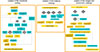 |
Fig. A.1. AGILE pipeline flowchart. Blocks from left to right describe the three main steps of the simulation: 1) The creation of the mock truth catalog which includes AGNs, galaxies and stars; 2) the creation of the instance catalogs obtained from the truth catalog by including variability information for AGNs and stars; 3) the creation of LSST single-visit images according to the LSST survey strategy, the reduction, and coaddition performed using the LSST Science Pipelines. This step also includes the photometric analysis (including forced photometry) which leads to the final photometric catalogs. |
Appendix B: Accuracy of extrapolation in p(λSAR)
As explained in Sect. 4.1, in order to assign λSAR to a complete Mstar > 108.5 M⊙ population of galaxies, we need to choose an extrapolation scheme. Choices for the extrapolation include boundary extrapolation (choosing the minimum and/or maximum value) or extrapolation with splines functions of varying degrees. In this work, we choose to extrapolate the parameter maps of Z24 by imposing a minimum Mstar = 109.5 M⊙ and maximum z = 4 where applicable. We compare this choice to the extrapolation scheme of scipy.interpolate.RegularGridInterpolator (Virtanen et al. 2020, version 1.16.2). This choice has the most consequences at z = 0.5, where differences in the chosen extrapolation can lead to a difference of 2.0 dex in p(λ), while the magnitude of the difference is smaller at higher z (see Fig. B.1).
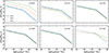 |
Fig. B.1. Accuracy of extrapolation in the assumed p(λSAR | Mstar, z, T) (Z24) using the parameter maps. The panels show different z, while the lines correspond to different Mstar as indicated by the legend. Dotted lines indicate extrapolation beyond the formal limits log10(Mstar/M⊙) < 9.5 or z > 4.0 using scipy.interpolate.RegularGridInterpolator. Given the uncertainties of the extrapolation (indicated most clearly in the top-left panel), in this work we choose to extrapolate by using they boundary values log10(Mstar/M⊙) = 9.5 and/or z = 4.0, corresponding to the blue solid curve (where applicable). |
Appendix C: QSOGEN posterior distribution parameters
We show the QSOGEN posterior distribution parameters (Sect. 4.4) in Fig. C.1.
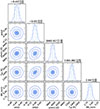 |
Fig. C.1. Posterior distribution of the five free QSOGEN parameters (Sect. 4.4), derived from a pure quasar sample with log10 (L5100 Å/erg s−1) ≥ 45.5. The contours represent the 1σ, 2σ, and 3σ confidence levels. The vertical lines show the 16%, 50%, and 84% percentiles, whose values are reported above each panel. |
Appendix D: AGILE first data release
Here we describe AGILE DR1, which is an application of the software in order to create an LSST-like array of simulated catalog-level products and images. The simulation has been run under Comitato di Allocazione di Tempo di calcolo e Spazio di archiviazione INAF (CAT&S) Pleiadi Call 5 with a total of 480 000 core hours awarded on the PLEIADI system of Trieste, Italy (Taffoni et al. 2020; Bertocco et al. 2020). The AGILE DR1 consists of the following output products:
-
Truth catalog of AGNs, galaxies and stars with an area of 24 deg2, 0.2 < z < 5.5, and log10(Mstar/M⊙) > 8.50, assuming the COSMOS2020 stellar mass function, and the specific accretion rate distribution from Z24 (Sects. 3, 4, and 5)
-
Truth SEDs of AGNs and galaxies in the optical/UV and NIR from 500 Å to 25 μm (Sect. 4),
-
Truth AGN ugrizy light curves with ten-year baseline and resolution of one day (Sect. 7),
-
Single-visit calexp and deep coadded ugrizy simulated LSST images corresponding approximately to 1 deg2 (21 / 189 detectors; Fig. D.1), and the first three years of LSST in COSMOS (1441 visits) using the modified baseline 4.0 (see Sect. 8)17,
-
Object catalog extracted from the deep coadded images (1 deg2, 1441 visits), including the best-match counterpart in the truth catalog (see Sect. 9),
-
Forced photometry catalog extracted from the single-visit calexp images (1 deg2, 1441 visits) at the positions of the object catalog detections (see Sect. 9),
-
The best-matching counterpart for each object catalog entry in the truth catalog.
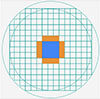 |
Fig. D.1. LSSTCam detector layout assumed in AGILE DR1. The LSSTCam consists of 189 detectors covering the full 9.6 deg2 FOV (the grid), and the commissioning camera used for LSST DP1 corresponds to nine detectors (blue region). For the purpose of reducing computational cost, for DR1 we choose to simulate a subset consisting of the central 21 detectors corresponding to a single-visit area of 1.1 deg2 (blue and orange regions). |
In addition, we provide python software (Jupyter notebooks) which demonstrates the usage and analysis of these data products. Updates concerning the AGILE DR1 and subsequent datasets are communicated through the main AGILE portal (https://www.oa-roma.inaf.it/lsst-agn/).
Appendix E: Catalog column descriptions
We show a complete listing of the truth catalog parameters in Table E.1. The columns in the photometric catalogs are detailed in the LSST Science Pipelines Software document (Vera C. Rubin Observatory Science Pipelines Developers 2025), Rubin Data Product definition document (https://lse-163.lsst.io/), and in the LSST Data Preview 0.2 documentation (https://dp0-2.lsst.io/data-products-dp0-2/index.html).
Parameters included in the truth catalog.
Appendix F: Photometric catalog flux accuracy measurements
We show the flux measurement accuracy from the AGILE DR1 object table for different classes in Table F.1 (see Sect. 9.2).
Flux measurement accuracy across classes of objects and flux definitions in the AGILE DR1 object catalog.
All Tables
Flux measurement accuracy across classes of objects and flux definitions in the AGILE DR1 object catalog.
All Figures
|
Fig. 1. Adapted distribution of λSAR of AGNs. Each panel shows p(λSAR | Mstar, z, T) at different Mstar (columns) and z (rows) values. The lines correspond to different combinations of AGN host galaxy type (quiescent or star forming) and AGN obscuration (CTN or CTK) in accordance with the legend. The specific Mstar and z values shown here have been selected for illustrative purposes, while the λSAR assignment follows the Z24 parameter maps as explained in Sect. 4.1. |
| In the text | |
|
Fig. 2. Resulting MBH–Mstar scaling relation from the continuity equation. Left: z evolution of the scaling relations from z = 0 (darker) to z = 5 (lighter). At each redshift, the dashed line style indicates the regime above the 99% stellar mass limits (assuming Weaver et al. 2023 COSMOS2020 stellar mass function and an area of 24 deg2), above which the MBH − Mstar relation is to be considered an extrapolation. The dotted line shows the assumed initial conditions at z = 5.5 (Reines & Volonteri 2015). Right: Local relation implied by the continuity equation (black line). The shaded region corresponds to an assumed scatter of Δlog10(MBH/M⊙) = 0.50 dex. The other non-solid lines correspond to local and inactive early-type galaxies (Häring & Rix 2004; Kormendy & Ho 2013), local AGNs (Reines & Volonteri 2015), the de-biased relation from SDSS galaxies (Shankar et al. 2016), and major-merger built S0 and E galaxies (Graham 2023). |
| In the text | |
|
Fig. 3. Simulated (red) and observed SDSS DR16 (black; Ahumada et al. 2020) colors versus z. Data and filters are from SDSS-DR16 (ugriz, Lyke et al. 2020), UKIDSS-LAS (YJHK, Lawrence et al. 2012), and unWISE (W1W2, Schlafly et al. 2019). For each z bin, 200 combinations of parameters were drawn from the posterior, the thickness of the line denotes the ±1σ region of the simulated colors. |
| In the text | |
|
Fig. 4. Examples of AGN (blue) and galaxy (red) SEDs in the observer frame. The black line shows the combined SED. Top (middle): Luminous Type 1 (Type 2) AGN. Bottom: LSST ugrizy transmission curves. |
| In the text | |
|
Fig. 5. X-ray luminosity function from the mock catalog compared to the literature. The panels correspond to different z values. The shaded region shows the XLF from the 24 deg2 mock catalog, while the green markers show the observed XLF compilation from various surveys (Shen et al. 2020). |
| In the text | |
|
Fig. 6. Mock truth catalog (24 deg2) g-band number counts for Type 1 and Type 2 AGNs, galaxies, and stars. The colored markers show values from the literature (LSST Science Collaboration 2009, Fig. 10.7). The triangles correspond to Hartwick & Schade (1990, up), Beck-Winchatz & Anderson (2007, left and down), and Richards et al. (2006, right), while the squares correspond to Wolf et al. (2003). The open triangle shows the QSONumberCountMetric for the COSMOS DDF (see the text for the details), while the open square shows the expected QSO number counts for the ten-year LSST survey (Li et al. 2025a). |
| In the text | |
|
Fig. 7. B-band quasar luminosity function. The shaded regions show the luminosity function of mock Type 1 AGN from the 24 deg2 truth catalog. The markers show the recent data compilation of the quasar luminosity function from Shen et al. (2020) at the redshift indicated by the text. |
| In the text | |
|
Fig. 8. Local active BHMF. Both the mock truth catalog (symbols) and observed (lines and shaded region; Ananna et al. 2022) active black hole mass functions correspond to Eddington ratios −3 < log10λ < 1. The mock λ is estimated from MBH and LX, assuming a constant bolometric correction LX / Lbol = 25. |
| In the text | |
|
Fig. 9. Example single-visit (calexp; left), deep coadd (middle) images, and the underlying truth catalog labels (right). The images correspond to the r-band with a small field of view of 2′ centered around |
| In the text | |
|
Fig. 10. Accuracy of the LSST Science Pipelines flux estimators for different classes of objects. Each panel shows the median (10th and 90th percentile) magnitude difference between the measured flux and the truth flux in the r-band. Rows correspond to the flux estimated using psfFlux, calibFlux (defined as the 12 pixel aperture flux), and cModelFlux, respectively. Columns correspond to the truth labels, as shown at the top of each column. |
| In the text | |
|
Fig. 11. Left: example light curves in the LSST bands of bright AGNs within AGILE DR1. The markers show psfFlux AGN light curves from the forced photometry catalogs, while the lines correspond to the truth catalog light curves in the same bands (indicated by the colors). As explained in the text and Appendix D, only the first exposure of each DDF sequence is shown, and the measured light curves span the first three years of simulated LSST operations in the COSMOS DDF according to baseline v4.0. Right panels: light curves only in the r-band of four bright AGNs. Otherwise, the axes and the units are the same as in the left panel. Top right: AGN (ID = 6289499) located close to the edge (< 1″) of the detector layout (Fig. D.1). It is sampled less frequently compared to the rest. |
| In the text | |
|
Fig. 12. Observed color-color diagrams using the LSST bands for detected AGILE sources. The markers and colors correspond to the labels of galaxies (or Type 2 AGNs), stars, and Type 1 AGNs in accordance with the legend, and corresponding to the true labels. A darker color is used to mark sources selected using the Croom et al. (2009) criteria. Only bright sources, g < 21.85 and i < 22, are shown. |
| In the text | |
|
Fig. 13. Magnitude versus RMS deviation in the r-band. Sources that are more than three times the MAD above the median of the distribution in a magnitude bin were selected as variable and labeled with red markers. Blue squares indicate Type 1 AGNs. The solid and dotted black lines represent the thresholds used to select variable sources for point-like and extended sources, respectively. |
| In the text | |
|
Fig. A.1. AGILE pipeline flowchart. Blocks from left to right describe the three main steps of the simulation: 1) The creation of the mock truth catalog which includes AGNs, galaxies and stars; 2) the creation of the instance catalogs obtained from the truth catalog by including variability information for AGNs and stars; 3) the creation of LSST single-visit images according to the LSST survey strategy, the reduction, and coaddition performed using the LSST Science Pipelines. This step also includes the photometric analysis (including forced photometry) which leads to the final photometric catalogs. |
| In the text | |
|
Fig. B.1. Accuracy of extrapolation in the assumed p(λSAR | Mstar, z, T) (Z24) using the parameter maps. The panels show different z, while the lines correspond to different Mstar as indicated by the legend. Dotted lines indicate extrapolation beyond the formal limits log10(Mstar/M⊙) < 9.5 or z > 4.0 using scipy.interpolate.RegularGridInterpolator. Given the uncertainties of the extrapolation (indicated most clearly in the top-left panel), in this work we choose to extrapolate by using they boundary values log10(Mstar/M⊙) = 9.5 and/or z = 4.0, corresponding to the blue solid curve (where applicable). |
| In the text | |
|
Fig. C.1. Posterior distribution of the five free QSOGEN parameters (Sect. 4.4), derived from a pure quasar sample with log10 (L5100 Å/erg s−1) ≥ 45.5. The contours represent the 1σ, 2σ, and 3σ confidence levels. The vertical lines show the 16%, 50%, and 84% percentiles, whose values are reported above each panel. |
| In the text | |
|
Fig. D.1. LSSTCam detector layout assumed in AGILE DR1. The LSSTCam consists of 189 detectors covering the full 9.6 deg2 FOV (the grid), and the commissioning camera used for LSST DP1 corresponds to nine detectors (blue region). For the purpose of reducing computational cost, for DR1 we choose to simulate a subset consisting of the central 21 detectors corresponding to a single-visit area of 1.1 deg2 (blue and orange regions). |
| In the text | |
Current usage metrics show cumulative count of Article Views (full-text article views including HTML views, PDF and ePub downloads, according to the available data) and Abstracts Views on Vision4Press platform.
Data correspond to usage on the plateform after 2015. The current usage metrics is available 48-96 hours after online publication and is updated daily on week days.
Initial download of the metrics may take a while.