| Issue |
A&A
Volume 691, November 2024
|
|
|---|---|---|
| Article Number | A355 | |
| Number of page(s) | 18 | |
| Section | Cosmology (including clusters of galaxies) | |
| DOI | https://doi.org/10.1051/0004-6361/202451755 | |
| Published online | 26 November 2024 | |
Examining the local Universe isotropy with galaxy cluster velocity dispersion scaling relations
1
Argelander-Institut für Astronomie (AIfA), Universität Bonn, Auf dem Hügel 71, 53121 Bonn, Germany
2
Leiden Observatory, Leiden University, PO Box 9513 2300 RA Leiden, The Netherlands
3
SRON Netherlands Institute for Space Research, Niels Bohrweg 4, NL-2333 CA Leiden, The Netherlands
4
University of California, Davis, CA 95616, USA
5
Center for Astrophysics | Harvard & Smithsonian, 60 Garden St., Cambridge, MA 02138, USA
6
INAF, Istituto di Astrofisica Spaziale e Fisica Cosmica di Milano, via A. Corti 12, 20133 Milano, Italy
7
Max Planck Institute for Extraterrestrial Physics, Giessenbachstrasse 1, 85748 Garching, Germany
8
Institut für Astronomie und Astrophysik Tübingen (IAAT), Sand 1, 72076 Tübingen, Germany
9
Korea Astronomy and Space Science Institute, Daejeon 34055, Republic of Korea
10
University of Science and Technology, Daejeon 34113, Republic of Korea
⋆ Corresponding author; apandya@astro.uni-bonn.de
Received:
1
August
2024
Accepted:
27
September
2024
Context. In standard cosmology, the Universe is assumed to be statistically homogeneous and isotropic. This assumption suggests that the expansion rate of the Universe, as measured by the Hubble parameter, should be the same in all directions. However, our recent study based on galaxy clusters finds an apparent angular variation of approximately 9% in the Hubble constant, H0, across the sky. In the study, the authors utilised galaxy cluster scaling relations between various cosmology-dependent cluster properties and a cosmology-independent property, i.e. the temperature of the intracluster gas (T). A position-dependent systematic bias of T measurements can, in principle, result in an overestimation of apparent H0 variations. Therefore, it is crucial to confirm or exclude this possibility.
Aims. In this work, we search for directional T measurement biases by examining the relationship between the member galaxy velocity dispersion and gas temperature (σv − T) of galaxy clusters. Both measurements are independent of any cosmological assumptions and do not suffer from the same potential systematic biases. Additionally, we search for apparent H0 angular variations independently of T by analysing the relations between the X-ray luminosity and Sunyaev-Zeldovich signal with the velocity dispersion, LX − σv and YSZ − σv.
Methods. To study the angular variation of scaling relation parameters, we determined the latter for different sky patches across the extra-galactic sky. We constrained the possible directional T bias using the σv − T relation, as well as the apparent H0 variations using the LX − σv and YSZ − σv relations. We utilised Monte Carlo simulations of isotropic cluster samples to quantify the statistical significance of any observed anisotropies. We calculated and rigorously took into account a correlation of LX and YSZ residuals.
Results. No significant directional T measurement biases are found from the σv − T anisotropy study. The probability that the previously observed H0 anisotropy is caused by a directional T bias is only 0.002%. On the other hand, from the joint analysis of the LX − σv and YSZ − σv relations, the maximum variation of H0 is found in the direction of (295 ° ±71 ° , − 30 ° ±71 ° ) with a statistical significance of 3.64σ, fully consistent with our previous results.
Conclusions. Our findings, based on the analysis of new scaling relations utilising a completely independent cluster property, σv, strongly corroborate the previously detected anisotropy of galaxy cluster scaling relations. The underlying cause, for example, H0 angular variation or large-scale bulk flows of matter, remains to be identified.
Key words: galaxies: clusters: general / cosmology: observations / large-scale structure of Universe / X-rays: galaxies: clusters
© The Authors 2024
 Open Access article, published by EDP Sciences, under the terms of the Creative Commons Attribution License (https://creativecommons.org/licenses/by/4.0), which permits unrestricted use, distribution, and reproduction in any medium, provided the original work is properly cited.
This article is published in open access under the Subscribe to Open model. Subscribe to A&A to support open access publication.
1. Introduction
Galaxy clusters are the largest gravitationally virialised systems in the Universe. They are crucial tools for astrophysical and cosmological studies as they provide valuable information about the large-scale structure and evolution of the Universe (Pratt et al. 2019). Galaxy clusters can be observed in multiple wavelengths, providing insights into different cluster properties. Galaxy cluster scaling relations describe the correlation between various important cluster properties using simple power laws (Giodini et al. 2013; Lovisari & Maughan 2022). These relations were predicted first by Kaiser (1986), and the model predicts that the objects of different sizes are merely scaled versions of each other. Due to this, it is also referred to as the self-similar model.
The evaluation of certain cluster observable properties involves cosmological assumptions. For instance, the X-ray luminosity (LX) and the total integrated Compton parameter (YSZ) rely on cosmological distances inferred from the estimated cluster redshift. The relation between these two quantities is a function of the assumed cosmological model. However, the measurement of some properties, such as intracluster gas temperature, T, and galaxy velocity dispersion, σv, depends very weakly on such cosmological assumptions. Valuable insights about different aspects of cosmology have been obtained by utilising the scaling relations between these two types of cluster properties (for a recent review, see Migkas 2024).
The cosmological principle is a fundamental assumption of the standard cosmological model, and it states that the Universe is homogeneous and isotropic on sufficiently large scales. The Friedmann equations – the basic set of equations that underpins most cosmological models – are derived under this assumption. The ΛCDM model assumes that matter should converge to an isotropic behaviour for cosmic volumes greater than 150 Mpc. This implies that the cosmic expansion rate, cosmological parameters, and the distances to extra-galactic objects depend solely on redshift, z, regardless of direction. Therefore, given the fundamental importance of this assumption, it is necessary to assess the validity of it.
The cosmic microwave background (CMB) observations support the cosmological principle within the CMB rest frame, exhibiting remarkable isotropy at small angular scales (Bennett et al. 1994, 2013; Planck Collaboration VI 2020). However, the CMB provides us with the rest frame of cosmic radiation in the early Universe, whereas examining the (an)isotropic behaviour of the matter rest frame in the local Universe (e.g. galaxies, clusters, and supernovae at z ≲ 0.5) through CMB data is particularly challenging and not extensively explored, with very few exceptions (e.g. Yeung & Chu 2022). Therefore, assessing if cosmic matter behaves isotropically in the local Universe is crucial. Additional cosmological probes are required to test the cosmological principle in the local Universe. Some of these probes include the use of Type Ia supernovae (SNIa) (Lopes et al. 2024; Zhai & Percival 2022; Hu et al. 2024), infrared quasars (Secrest et al. 2021), the distribution of optical (Javanmardi & Kroupa 2017; Sarkar et al. 2019) and infrared galaxies (Yoon et al. 2014; Rameez et al. 2018) and the distribution of distant radio sources (Singal 2011; Rubart & Schwarz 2013; Tiwari & Nusser 2016; Colin et al. 2019) and gamma-ray bursts (Řípa & Shafieloo 2017; Andrade et al. 2019).
Previous studies have returned ambiguous results, with some identifying apparent anisotropies while others report consistency with the isotropy hypothesis. For instance, Lopes et al. (2024) find significant dipole variation of the H0 at more than 99.9% confidence level, Secrest et al. (2022) reject the cosmological principle at 5.1σ, and Colin et al. (2019) detect a 3.9σ anisotropy in the deceleration parameter. Other studies report apparent anisotropies with moderate or low statistical levels. For example, Haridasu et al. (2024) find ΔH0/H0 ≲ 3% at a confidence level of 95%, and Mc Conville & Colgáin (2023) find H0 angular variations up to 4 km s−1 Mpc−1 at a statistical significance up to 1.9σ. At the same time, Wagenveld et al. (2024), Soltis et al. (2019), Andrade et al. (2019) report no deviation from the isotropy hypothesis at large scales. However, many of these studies suffered from inhomogeneous sky coverage, which may have led to an underestimation of the detected anisotropy.
Galaxy clusters have become a useful tool to test the cosmological principle in recent years. A new method based on cluster scaling relations was introduced by Migkas & Reiprich (2018). Migkas (2020) (hereafter M20) and Migkas et al. (2021) (hereafter M21) then applied various scaling relations for galaxy clusters to examine the isotropy of the local Universe quantitatively. The key principle behind these studies involved pairing a cosmology-dependent quantity (e.g. LX and YSY) with the cosmology-independent T. This pairing allowed them to draw conclusions on the directionality of cosmological parameters. They find a (9.0 ± 1.7)% variation in the Hubble constant (H0) across the sky which could be alternatively attributed to a ∼900 km s−1 cluster bulk flow extending up to ∼500 Mpc (z ∼ 0.12). These results strongly disagree with the isotropy assumption underlying the standard model of cosmology (ΛCDM) (for a recent review, see Migkas 2024).
Galaxy cluster T is a measure of the average kinetic energy of the electrons in the hot intra-cluster medium (ICM) and is measured using X-ray spectroscopy. However, there is a possibility that such T measurements could be affected by systematic biases and, eventually, bias cosmological conclusions. Indeed, it has long been known that X-ray T measurements may be biased in various ways (see, e.g. Chapter 4 in the review by Reiprich et al. 2013). However, an angular variation of such a bias is not expected. Possible reasons for directional-dependent systematic biases include under or overestimation of absorption corrections in T in certain directions. However, this effect would likely be very small, as we used a range of 0.7 − 7 keV for the T measurement. Another potential factor could be the presence of a hot, diffuse cloud that is not accounted for in the X-ray background. Regardless, if present, such a direction-dependent bias may lead to variations in best-fit parameters of scaling relations that depend on sky position. If the variations observed by M20 and M21 were indeed due to such systematic biases, a ∼10 − 13% overestimation of T towards the most anisotropic direction identified by M21 could alleviate the tension between their findings and the ΛCDM model1. Therefore, it is essential to carefully investigate systematic T biases in the data used by M21 throughout the whole sky.
In this work, we look for potential T measurement biases across the sky by pairing the cluster T with the σv since its measurement also does not involve any cosmological assumptions. We convert the variations obtained in the σv − T relation’s best-fit parameters into T over- or underestimations across the sky. σv has completely different systematics as compared to T but is unaffected by Galactic absorption. Therefore, if the latter is the reason for a possible T bias, this will, in principle, show up in this scaling relation’s anisotropy. A significant variation in the best-fit normalisation across the sky that results in a noticeable overestimation of T in a particular region would suggest that systematic biases influence the results reported in M21. Conversely, if the best-fit parameters are uniform across the sky, it implies that a systematic T bias is a highly unlikely explanation for the observed anisotropies in M21.
We also explore cosmic isotropy by using σv in combination with cluster properties, whose measurements rely on cosmological parameters. Two scaling relations, the X-ray luminosity-velocity dispersion (LX − σv) and the total integrated Comptonization parameter-velocity dispersion (YSZ − σv), are studied for this purpose. The variations in the best-fit parameters of these relations are converted to variations in H0. This test provides new insights into a potential H0 angular variation (or H0 anisotropy) and acts as a cross-check of the M21 results. For this work, a flat ΛCDM model is assumed with H0 = 70 km s−1 Mpc−1, Ωm = 0.3 and ΩΛ = 0.7.
The paper is structured as follows: Section 2 describes the various data samples and cluster properties used in this work. Section 3 explains the fitting procedure for scaling relations and the techniques used to study their variations across different parts of the sky. In Sect. 4, we present the general behaviour of the scaling relations used in this work. Section 5 provides detailed information on the variations in the best-fit parameters of the σv − T relation, T bias across the sky, and the isotropic Monte Carlo simulation results. Section 6 explores the variations of LX − σv and YSZ − σv scaling relations, H0 variations across the sky from their joint analysis, and their comparison with isotropic Monte Carlo simulations. In Sect. 7, we discuss possible systematics and compare our results with M21. Finally, in Sect. 8, the conclusions of this work are given.
2. Data samples
This work utilises four key cluster parameters: T, σv, LX, and YSZ. These parameters are obtained for clusters present in three different data catalogues: the Meta Catalogue of X-ray detected Clusters of galaxies (MCXC, Piffaretti et al. 2011), the extremely expanded HIghest X-ray FLUx Galaxy Cluster Sample (eeHIFLUGCS, Pacaud et al., in prep.), and the Euclid velocity dispersion metacatalog (Euclid Collaboration: Melin et al. 2024, in prep.).
MCXC is a comprehensive catalogue of X-ray-detected galaxy clusters, which is based on the ROSAT All-Sky Survey (RASS). For each cluster, the catalogue provides the position, redshift, standardised 0.1 − 2.4 keV band luminosity LX = L500, total mass M5002, and radius R5003. eeHIFLUGCS is a homogeneously selected sample of galaxy clusters that was created by imposing several selection criteria on the MCXC, such as a flux limit on the unabsorbed X-ray flux and the availability of a high-quality Chandra (Weisskopf et al. 2000) or XMM-Newton (Jansen et al. 2001) observation. The catalogue also contains homogeneously calculated cluster T. The Euclid velocity dispersion metacatalog is a collection of homogeneous velocity dispersion measurements from various sources compiled by the Euclid Collaboration. The catalogue includes clusters from previous catalogues such as the Planck cluster sample (Aguado-Barahona et al. 2022), Abell (Girardi et al. 1998), ACO (Mazure et al. 1996), XDCP (Nastasi et al. 2014), SDSS/Abell (Popesso et al. 2007), and other samples.
2.1. X-ray luminosity LX and temperature T
We utilised the LX from the eeHIFLUGCS catalogue, which contains the luminosity measurements from the RASS (Voges et al. 1999) covering the entire R500 of a cluster. This is different from most of the XMM-Newton and Chandra clusters available in this catalogue. The luminosities of the MCXC have been corrected for the Galactic absorption based on the Willingale et al. (2013)NHtot values as described in M21. The LX values are available for 380 clusters in the eeHIFLUGCS catalogue.
The cluster T data was sourced from the eeHIFLUGCS catalogue, as provided in Migkas (2020). The T values were measured within the range of 0.2 − 0.5 R500 for each cluster and were derived from observations made by Chandra and XMM-Newton. In total, T values are available for 313 eeHIFLUGCS clusters.
2.2. Total integrated Compton parameter YSZ
The Sunyaev-Zeldovich (SZ) effect provides information about the total gas pressure of the ICM and is characterised by the Compton parameter denoted by the symbol y. The integrated Compton parameter Y is obtained by integrating y over the cluster’s solid angle. This quantity is multiplied by the square of the angular diameter distance to obtain the total integrated Compton parameter YSZ, which has units of kpc2, and scales with other cluster properties (detailed description available in M21).
We determined YSZ values for all MCXC clusters using the final data release of Planck Collaboration I (2020) as explained in M21. We applied several signal-to-noise (S/N) cuts to the YSZ measurements to see how our results depend on the YSZ selection. For the default analysis, we used an S/N cut of ≥2, which resulted in 1093 clusters being included. Results in Sect. 6.5 show that no systematic trends are observed when we vary the S/N cut. We are already aware of the existence of clusters in these areas. Therefore, there was no necessity to increase the S/N cut for detection purposes.
2.3. Velocity dispersion σv
The velocity dispersion of a galaxy cluster is a measure of the spread of velocities among the member galaxies of the cluster. It is obtained by measuring the line-of-sight velocities of the member galaxies in optical bands. We utilised the Euclid velocity dispersion metacatalog for the σv measurements. This catalogue includes 614 clusters and has several important properties: Firstly, all the clusters have at least ten member galaxies with spectroscopic redshift measurements, and interlopers were adequately rejected while defining cluster members. Secondly, the velocity dispersion calculations were based on the methodology of Beers et al. (1990) with a S/N ≥ 4 and a minimum aperture of 0.5 Mpc. In addition to the velocity dispersion errors from the parent catalogues, dispersion uncertainties were also calculated in a standard way (Sereno & Ettori 2015).
2.4. Matching different catalogues
We cross-matched the σv catalogue to eeHIFLUGCS and the YSZ data (MCXC clusters) to study various scaling relations. Our primary matching criteria were that the cluster positions should be within 5′ of each other, and the difference in redshifts Δz of the matching clusters should not exceed 0.01. We discovered 165 matching clusters with both σv and T measurements and 200 clusters with both LX and σv measurements for the eeHIFLUGCS sample. We identified 284 matching clusters between the σv catalogue and the YSZ data (S/N ≥ 2). Table 1 summarises the scaling relations used along with the number of clusters associated with each relation.
Best-fit parameters for the three scaling relations for the full sample.
3. Analysing the scaling relations
To study the three distinct scaling relations, a general form of the scaling relation was adopted. The scaling relation between two variables, Y and X, is expressed as
Here CY and CX are the pivot points for the Y and X quantity respectively, E(z) is the redshift evolution factor  with γYX being its power law index. AYX and BYX are the normalisation and slope of the scaling relation, respectively. The pivot points CY and CX are chosen close to the median of the Y and X, respectively. This was done to minimise the correlation between the best-fit parameters. These terms and the γYX for all three scaling relations are mentioned in Table 1.
3.1. Bayesian linear regression
A linear regression was performed using Bayesian statistics to find the best-fit parameters for scaling relations in the logarithmic space. We constrained the best-fit parameters by maximising the posterior probability distribution of the parameters. The Markov Chain Monte Carlo (MCMC) method was used for sampling these distributions. We took its logarithm to convert the power law relation to a linear relation. The general form of scaling relations in terms of a linear model is given as
where  ,
,  , m = BYX, and c = log10(AYX).
To speed up the calculation process, the logarithm of the posterior probability distribution was used. The log-likelihood function is given as
![$$ \begin{aligned} \log \left( \mathcal{L} \right) = -\frac{1}{2} \sum _{i = 1}^{N} \left( \frac{[y_i - mx_i - c]^2}{\sigma _i^2} + \log \left( 2\pi \sigma _i^2 \right)\right), \end{aligned} $$](/articles/aa/full_html/2024/11/aa51755-24/aa51755-24-eq15.gif)
where N is the number of data points, yi and xi are the ith data points of Y and X respectively, and σi is the total uncertainty given by:
Here σy, i and σx, i are the uncertainties4 for the yi and xi, respectively, and σintr is the intrinsic scatter of the scaling relation measured in Y direction. Thus, the three parameters to be constrained are m, c, and σintr. Flat priors were used for m and c with upper and lower bounds of +10 and −10, respectively. Since σintr is a positive definite quantity, a flat prior with a lower bound of 0 and an upper bound of +10 was selected. Even though the prior choices are uninformative, the resulting posterior distribution always converges to a normal distribution.
The chain was initialised with a random set of parameters. It was run for at least 20 000 iterations in four chains to ensure it converged5. The best-fit parameters were obtained by taking the median of the parameter space distribution. Lower and upper bounds were then determined by using the 16th and 84th percentile values of the distribution, respectively. The implementation of Bayesian linear regression was coded in Python6 and the numba (Lam et al. 2015) package was used to improve computational time. The validity of the code was verified by comparing the results with the LINMIX (Kelly 2007) and PyMC (Abril-Pla et al. 2023) packages, and we find results that are consistent.
This method for Bayesian linear regression is Y|X since the y-axis distance of the data points from the best-fit line is minimised, and x is treated as the independent variable. For certain scaling relations, X|Y best-fit implementation was used (more details in Sect. 4). In this method, the x-axis distance of the data points from the best-fit line is minimised, and y is treated as the independent variable. The log-likelihood function for X|Y is given as
![$$ \begin{aligned} \log \left( \mathcal{L} \right)_\mathrm{X|Y} = -\frac{1}{2} \sum _{i = 1}^{N} \left( \frac{\left[x_i - \left(\frac{y_i - c}{m}\right)\right]^2}{\sigma _{i, \mathrm{X|Y} }^2} + \log \left( 2\pi \sigma _{i, \mathrm{X|Y} }^2 \right)\right), \end{aligned} $$](/articles/aa/full_html/2024/11/aa51755-24/aa51755-24-eq17.gif)
where σi, X|Y is  . The σintrX|Y is the intrinsic scatter of the scaling relation measured in X direction. Note that the slope m and the normalisation (10c) refer to the best-fit parameters of the Y|X form of the relation (LX − σv), and not to the X|Y form (σv − LX).
3.2. Removing outliers
We used an iterative 3σ clipping method to detect and remove outliers in the data. This method removes outliers based on their residual distance from the best-fit line. In the Y|X fitting method, residuals are considered in the Y direction, while in the X|Y method, residuals are considered in the X direction. The method assumes that residuals follow a normal distribution, and points lying outside the 3σ of this distribution were removed as outliers. Using the 3σ cut, we expect approximately one out of every 370 clusters to fall outside this range purely due to chance. Since the number of clusters in all relations is less than 370, we could safely use the 3σ cut. This approach did not eliminate any clusters that adhere to normal scaling relation behaviour and helped eliminate problematic measurements.
It is important to note that this method may remove additional outliers when repeated because the new sample will have different best-fit parameters, resulting in different residual distributions. The method was repeated several times until no new outliers were found. Typically, this method removes 2–5 outliers from each scaling relation sample. Table 1 lists the final sample sizes for the scaling relations. Fig. 1 displays the sky distribution of the clusters used in the scaling relations σv − T, LX − σv, and YSZ − σv, along with their redshifts.
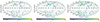 |
Fig. 1. Sky distribution of the galaxy clusters used in the scaling relations σv − T (left), LX − σv (middle), and YSZ − σv (right). The clusters’ redshifts are colour-coded. |
3.3. Scanning the sky
We studied the consistency of the scaling relations in different sky directions by considering sections of the sky and calculating the best-fit parameters of the clusters inside those regions. We used the two-dimensional scanning method adopted from M21. In this method, a cone of radius θ was constructed for a given galactic longitude l and latitude b, and the scaling relation best-fit parameters of the clusters inside this cone were constrained. To cover the entire sky, the central longitudes and latitudes of the cones were varied with a step size of 5° for their whole range. This results in 72 × 37 = 2664 different cones covering the entire sky7. Ideally, the cone sizes should be as small as possible to minimise overlap. However, the cone size should also be large enough to have sufficient clusters8 inside the cone to efficiently constrain the best-fit parameters. We tested various cone sizes and found a cone size of radius θ = 75° to be optimal for this analysis (additional details in Appendix A). An example of such a cone, along with the statistical weights of clusters inside this cone for the σv − T sample, is shown in the bottom panel of Fig. 2.
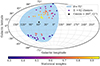 |
Fig. 2. Example of a region used for two-dimensional scanning centred at (l, b) = (60 ° ,15 ° ) with cone size, θ, of radius 75° for σv − T relation. Different colours represent the statistical weights assigned to the clusters inside these regions. ∑ represents the number of clusters inside this region. |
We also applied statistical weights to clusters inside the scanning regions. This was done by dividing the statistical uncertainties of the observables (σy and σx) by the cosine of the angular separation of the cluster from the cone centre9. This results in a lower statistical weight for clusters that are further from the cone centre. 2D maps are created to visualise the results of 2D scanning. These maps are a grid plot with a box size of 5° on the Aitoff projection of the sky using the Python package desiutil10. The colour of each box in these maps represents the parameter value of interest for the cone centred at a given l and b.
3.4. Constraining H0 angular variations
In the analysis of LX − σv and YSZ − σv scaling relations, we assumed that the intracluster physics remain unchanged for different directions, and variations of cosmological parameters cause the apparent anisotropy of scaling relations. According to this assumption, H0 can vary across the sky while the true normalisation of the scaling relations remains constant. Alternatively, the A variations can also be interpreted in other ways, such as the presence of large-scale bulk flows, as shown in M21. However, due to the large scatter in the scaling relations, we restricted our analysis to constraining H0 angular variations.
We used best-fit A/Aall of every cone to constrain H0 angular variations using the relation
Here H70 = 70 km s−1 Mpc−1 and Aall is the best-fit A of the entire sample. A and H0 are degenerate, and absolute constraints can only be put on the quantity A × H02. One of these parameters is assumed to be fixed to constrain the other (more details in Appendix F). This method cannot be used to put absolute constraints on H0 because a value of H0 was assumed to calibrate the relation initially. The calculated value of H0 expresses relative differences between the regions; thus, the variations are always around the assumed value of H0.
3.5. Statistical significance of the variations
We used the best-fit parameters and their uncertainties in different parts of the sky to quote the nominal statistical significance of the variations between the two regions. For two independent sub-samples i and j, the nominal statistical significance of their deviation in terms of number of sigma is given by
where pi and pj are the best-fit parameters of the two sub-samples, and σpi and σpj are their uncertainties. For a cone centred at (l, b), all the clusters inside it were considered one sub-sample, and the clusters outside the cone were considered the other sub-sample. We find the nominal significance values for each cone to create a nominal significance (sigma) map. The colour of each box in this map represents the nominal statistical significance of deviation compared to the rest of the sky at that location.
3.6. Isotropic Monte Carlo simulations
The statistical methods used above provide a way to study the anisotropies in the scaling relations. However, unknown statistical biases could still be present in the analysis methods, which could lead to under- or overestimation of the significance of anisotropies. We performed isotropic Monte Carlo simulations to test the method’s validity and provide robust significance. To create an isotropic sample for a scaling relation, we performed the following steps:
-
We started by fixing the cluster coordinates, redshifts, and σv (including the uncertainties) to their actual values. This was done to encompass potential effects that may give rise to anisotropies, including the spatial arrangement of real clusters.
-
The cluster T, LX, and YSZ were simulated based on the best-fit parameters and scatter of the real data. First, their predicted values corresponding to the fixed σv were calculated using the respective best-fit parameters.
-
Once all the points lie on the best-fit line, a random offset was added to these predicted values to obtain a simulated sample. This was done by drawing random values from a log-normal distribution centred at this value with a standard deviation equal to the total scatter (intrinsic + statistical) of the respective scaling relation and given cluster.
-
Step 3 was repeated 1000 times, each time adding a random offset to the predicted values to create 1000 simulated samples.
We compared the maximum variations in scaling relations across the sky for these samples with those obtained from the observations to quantify the statistical significance of the observed differences against random chance.
4. General behaviour of the three scaling relations
The three scaling relations used were σv − T, LX − σv, and YSZ − σv. This section presents best-fit parameters for these scaling relations for the entire sample. These relations are plotted in Fig. 3, and Table 1 shows an overview of the best-fit results. The number of matching clusters here differs from that mentioned in Sect. 2.4 due to the removal of outliers, as described in Sect. 3.2.
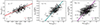 |
Fig. 3. Best-fit plots for the three scaling relation. The shaded regions represent 1σ uncertainties of the best-fit parameters. From left to right:σv − T (Y|X), LX − σv (X|Y), and YSZ − σv (X|Y) relations. |
4.1. σv − T relation
To study the σv − T relation, 160 galaxy clusters with measured velocity dispersion and temperatures were used. We obtained a best-fit slope of  , which is lower than the predicted self-similar value of 0.5 (Lovisari et al. 2021). Recent studies (Xue & Wu 2000; Ortiz-Gil et al. 2004; Nastasi et al. 2014; Wilson et al. 2016) obtain a slightly higher slope than the predicted self-similar scaling relation. One important thing to note is that most previous studies use the Orthogonal Distance Regression (ODR) method to fit the data. In contrast, Y|X was used for this analysis, which usually returns a flatter slope than ODR. Using the ODR method for our sample, a slope of
  is obtained, similar to the results from Y|X but slightly larger.
4.2. LX − σv relation
195 clusters were used to study LX − σv relation. The X|Y method was used to get best-fit parameters since the Y|X method results in residual trends when plotted against the cluster redshifts (refer to Appendix B for more details). However, as shown in Sect. 6.5, the choice of fitting method does not significantly influence the final results.
Using the X|Y method we find  while the Y|X leads to a shallower slope
  . The slope from the Y|X method is similar to the self-similar slope Bself = 2.7 − 2.8 when considering 0.1 − 2.4 keV luminosities for clusters (Lovisari et al. 2021). Previous studies (Mahdavi & Geller 2001; Ortiz-Gil et al. 2004; Zhang et al. 2011; Nastasi et al. 2014; Sohn et al. 2019) using bolometric luminosities for clusters have obtained slopes consistent with the predicted slope of Bself = 4. Most of these studies use the ODR method to fit the data. We obtain similar results using X|Y and ODR methods.
4.3. YSZ − σv relation
For the relation YSZ − σv, 284 clusters were used. These clusters were selected based on S/N ≥ 2 for the YSZ parameter. The theoretical slope using the self-similar model is Bself = 5 (derived from Lovisari et al. 2021). This is different from what is observed as, using X|Y, we find a steeper slope  , and Y|X leads to a shallow slope
  . These trends are similar to what was observed in the LX − σv relation. Previous results from Rines et al. (2016) are quite similar to those obtained for X|Y and Y|X with a slope of 5.68 ± 0.64 and 2.36 ± 0.30, respectively.
5. Measuring the systematic temperature bias
To perform systematic checks on the T measurements using σv − T, we studied the 2D variations and the best-fit results are converted to T over- or underestimation. The statistical significance of the analysis is checked using the isotropic Monte Carlo simulations.
5.1. Two-dimensional variations
The 2D variations of best-fit parameters were studied by shifting a cone of radius 75° across the sky. The left panel of Fig. 4 shows maps of the best-fit A and B in different regions compared to the full sample (Aall and Ball respectively). Maps for A/Aall show values within a few per cent of 1, suggesting no substantial variations. To comment on the nominal statistical significance of the variations, nominal significance maps for A and B were created (right panel of Fig. 4). The nominal significance maps for A show that the most deviating region is (l, b) = (195 ° , − 20 ° ) with a nominal significance of 2.27σ. This region deviates from the rest of the sky by 7.20 ± 3.49%.
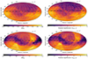 |
Fig. 4. Left panel: maps of best-fit normalisation (top) and the slope (bottom) compared to the full sample for the σv − T relation. Note that the colour scale is different for both maps. This highlights the small variations in the A/Aall map. Right panel: nominal significance maps for the normalisation (top) and slope (bottom). Both maps have the same colour scale (−3σnom to +3σnom). A negative sigma value refers to a value lower than the rest of the sky. |
The nominal sigma maps for B show that the most deviating region is (l, b) = (65 ° , − 25 ° ) with a nominal significance of 2.42σ. The variations obtained in the best-fit slopes have a slightly higher nominal significance, but the most deviating region is still well below 3σnom. These nominal significance estimates already lead us to conclude that no significant variations are detected in the σv − T relation. The statistical insignificance of the σv − T angular variations is further confirmed in Sect. 5.3.
5.2. Temperature bias
We performed the following steps to convert the variations in best-fit normalisation into T bias. To quantify the change in T for a given σv = A × TB across the sky, we used
We took Region One as the region of interest and Region Two as the rest of the sky. The value of B is the best-fit slope for the rest of the sky and was assumed to be the same for both regions. The quantity ΔT = T1 − T2 is the temperature bias between a region and the rest of the sky. We quantified this in terms of percentage bias using the relation
A 2D map of %T bias was created to identify regions with over- or underestimation of T (Fig. 5). Since ΔT was calculated from A, the region of most bias remains the same. This region shows a (16.3 ± 7.1)% underestimation in T compared to the rest of the sky. There are notable T biases across the sky in the 2D map, indicating anisotropy. However, these are also accompanied by high uncertainty and already the nominal significance analyses above have shown they are not significant. Note that here, the region with the largest deviation from isotropy in M21 has an insignificant but nonetheless negative T bias. In contrast, a positive bias would be needed to alleviate the anisotropy in M21.
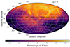 |
Fig. 5. Map of percentage T bias between a region and rest of the sky. Negative T variations refer to an underestimation of T compared to the rest of the sky. To alleviate the observed anisotropies in M21, the behaviour required would have to be opposite to what is observed. |
5.3. Isotropic Monte Carlo simulations
Isotropic Monte Carlo simulations were performed for the σv − T scaling relation to check the validity of the methodology used to obtain the results from the 2D analysis and to obtain improved significance estimates. Isotropic samples were created using the method mentioned in Sect. 3.6. For these simulated samples, nominal significance maps were created using the same procedure as the real data, and the maximum nominal significance value was noted. We also took note of its corresponding percentage T bias to understand the expected T bias solely due to the statistical scatter of the relation. It is important to note that an isotropic sample with a large scatter around the best-fit line will exhibit a T bias. We can assess the statistical significance of the obtained bias by comparing the expected T bias from the scatter and the real data. The distribution of these quantities obtained from the simulations is shown in Fig. 6. Since the maximum variation in the observed data corresponds to a negative T bias, we plotted only the negative T bias values from the simulations for their comparison.
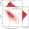 |
Fig. 6. Distribution of maximum nominal sigma values and its %T bias obtained from the 1000 isotropic Monte Carlo simulated samples of the σv − T relation. Shaded contours represent 68%, 95%, and 99% confidence levels. The value obtained in the real data is shown by a black dashed line on the histograms and by a point on the contour plot. The p-value in the histogram of maximum nominal sigma values represents the probability of getting higher nominal significance than the real data. |
The figure shows that the probability of obtaining a nominal sigma value of 2.27σ or higher is 72% (p = 0.72), and ∼18% bias in T is expected purely due to the scatter of the relations. The 2D distribution of these simulated results demonstrates that real data lies well within the 68% confidence interval, indicating a high probability of such results occurring due to statistical fluctuations. These results further confirm that the variations in the best-fit normalisation (and, therefore, T biases) are not statistically significant.
6. Probing cosmic anisotropies
In this section, we present the constraints of the apparent H0 anisotropies using the LX − σv and YSZ − σv relations. We cross-checked the results of M21 with an independent cluster property that is different from that used in the original study.
6.1. LX − σv relation
Using 2D scanning, we find A variations across the sky and compare them with A of the full sample (Aall). The 2D maps of A/Aall along with nominal significance maps are shown in Fig. 7. The nominal sigma maps for A show that the most deviating region is (l, b) = (225 ° ±41 ° , − 25 ° ±41 ° ) with a nominal significance of −3.66σ. Some variations in the best-fit slopes are also observed in certain regions but at a lower nominal significance. However, slope variations are not a focal point of this test as they do not strongly affect the inferred H0 variations (no strong correlation exists between slope and H0 constraints).
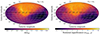 |
Fig. 7. Map of best-fit A compared to the full sample (left) and its nominal significance map (right) for the LX − σv relation. |
The H0 angular variation map obtained from the LX − σv relation is shown in Fig. 8. The region exhibiting the most statistically significant deviation remains consistent with the A maps. In terms of H0, this region differs from the rest of the sky by ΔH0 = 28.3 ± 6.6%.
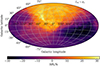 |
Fig. 8. H0 angular variation map created from the LX − σv relation. |
In order to better understand the variation in data points (i.e. individual clusters) between the region of maximum anisotropy (l = 225 ° ,b = −25 ° ) and the rest of the sky, we created a distribution of H0 values corresponding to the data points in these regions and compared them with each other (see Fig. 9). We assigned a value of H0 to each data point based on its vertical distance from the best-fit line. Points on the line were assigned H0 = 70 km s−1 Mpc−1. The H0 value for a point with a y value of yi and the best-fit y = yfit was calculated using the formula  . On average, data points in the region (l = 225 ° ,b = −25 ° ) tend to have lower H0 and thus lie below the best-fit line. The rest of the sky contains a larger number of data points that lie above the best-fit line, as observed from the distribution tail.
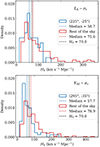 |
Fig. 9. Distribution of H0 values corresponding to each data point in the region of maximum anisotropy and rest of the sky for the relations LX − σv (top) and YSZ − σv (bottom). The median of both distributions is shown by dashed lines along with H0 = 70 km s−1 Mpc−1. Note that both regions have different numbers of clusters, and thus, to compare both, the density of the distribution is plotted. |
6.2. YSZ − σv relation
Fig. 10 shows the maps of best-fit A of different regions compared to the full sample and their sigma maps. The direction showing the largest A deviation is (l, b)∼(295 ° ±58 ° , − 35 ° ±58 ° ) with a nominal statistical significance of −4.13σ. This is in a similar direction to the most deviating region in the LX − σv analysis.
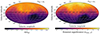 |
Fig. 10. Map of best-fit A compared to the full sample (left) and its nominal significance map (right) for the YSZ − σv relation. Both maps have the same colour scale as Fig. 7. |
One interesting feature of this map is that, on average, the Northern Galactic Hemisphere shows higher A values than the Southern one. The best-fit A of all the clusters in the two Galactic Hemispheres differs by 3.35σ. We were unable to identify a systematic bias causing this phenomenon; therefore, it is plausible that this discrepancy may be a random occurrence. We tested the possibility of assuming an incorrect redshift evolution factor and its effects on detecting anisotropy and this feature in Sect. 7.4.
The H0 angular variation maps that are derived from the YSZ − σv relation are shown in the Fig. 11. The region exhibiting the most statistically significant deviation differs from the rest of the sky by ΔH0 = 28.5 ± 6.4%. The H0 distributions in the region of maximum anisotropy (l = 295 ° ,b = −35 ° ) and the rest of the sky (Fig. 9) reveal a similar distribution to the ones obtained from LX − σv analysis.
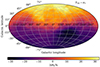 |
Fig. 11. H0 angular variation map created from the YSZ − σv relation. The map has the same colour scale as Fig. 8. |
6.3. Joint analysis of LX − σv and YSZ − σv relations
The apparent anisotropy information of the LX − σv and YSZ − σv scaling relations can be combined into one map that shows H0 angular variations. By multiplying the H0 posterior probability distributions of the two relations, the combined H0 posterior probability distribution can be obtained. By using the combined posterior probability distribution to constrain the best-fit H0 for each cone, we generated a combined map showing the percentage change in H0 and its nominal significance.
6.3.1. Limitations of joint analysis
There are a couple of things to note here that could overestimate the nominal significance of the detected anisotropies. First, we assume there is no bias in σv measurements. Since it is used in both the scaling relations, a bias could overestimate the significance. Second, this method of combining the likelihoods assumes there is no correlation between the scatter of LX and YSZ at fixed σv.
Previous studies like Nagarajan et al. (2019) have shown a positive correlation between the scatter. We have 180 clusters with both LX and YSZ measurements, and we used them to find the correlation between their scatter from their respective scaling relation. Fig. 12 shows a plot of residuals of the two relations along with their best-fit line. The correlation coefficient between the residuals is 0.957, and the best-fit slope of 1.01 ± 0.04. The strong correlation could be the result of a large scatter/uncertainty in σv, causing the cluster to shift in the same direction for both the LX − σv and YSZ − σv relations. Despite a correlation, ∼37% clusters present in YSZ − σv are unique to this relation and are completely independent of the LX − σv relation.
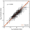 |
Fig. 12. Correlation between the residuals of the relations LX − σv and YSZ − σv. The best-fit line is shown in orange, along with the correlation coefficient. |
6.3.2. Apparent H0 anisotropy from joint analysis
The joint H0 map and its nominal significance maps are shown in Fig. 13. The region with the most deviation is found to be in the direction of (l, b)∼(295 ° ±71 ° , − 30 ° ±71 ° ) with ΔH0 = 27.6 ± 4.4% and nominal statistical significance of −5.27σ compared to the rest of the sky. Notice that the nominal significance of the variation has increased compared to the individual analysis, which is a result of smaller H0 uncertainties. The strong correlation between the residuals suggests that the two relations are clearly not independent and that simply combining the likelihoods will undoubtedly result in overestimating the nominal significance.
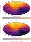 |
Fig. 13. H0 angular variation maps created from the joint analysis of relations LX − σv and YSZ − σv (top) and its nominal significance map (bottom). Colour scales for the H0 angular variation map are the same as before, but the colour scales for the sigma map have been increased to account for increased significance. |
6.4. Isotropic Monte Carlo simulations
We performed isotropic Monte Carlo simulations by considering the residual correlation to calculate realistic significance. The method for creating an isotropic MC simulated sample is described in the Sect. 3.6.
First, we generated simulated LX and YSZ values based on the best-fit line, taking into account the total scatter of their respective relations. However, simulated YSZ values were calculated only for clusters that are unique in the YSZ − σv dataset. For the 180 clusters that have both LX and YSZ values, we obtained simulated YSZ by taking into account the correlated scatter of LX and YSZ with σv. To do so, we started by determining the residuals of YSZ that correspond to residuals of the simulated LX using the correlation between the two quantities (Sect. 6.3.1). These residuals were then used to predict YSZ by applying the best-fit parameters of the YSZ − σv relation. Finally, a random offset was added to these values, which was drawn from a log-normal distribution centred at YSZ, pred and the standard deviation of  .
.
This was done 1000 times to create 1000 simulated LX and YSZ samples. The distribution of maximum nominal sigma values and ΔH0 variations obtained from the simulations were compared with the real data in Fig. 1411. We examined the isotropic sample’s ΔH0% corresponding to maximum nominal sigma values to know the expected ΔH0 caused by the spread in the scaling relation. A large scatter in the scaling relation leads to significant ΔH0 when considering its sub-samples. Therefore, by comparing ΔH0 obtained from isotropic samples and the real data, we can assess the significance of these variations given the scatter in the relation.
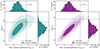 |
Fig. 14. Distribution of maximum nominal sigma values and its ΔH0 variations obtained from the 1000 isotropic Monte Carlo simulated samples of the LX − σv (left) and YSZ − σv (right) relations. Shaded contours represent 68%, 95%, and 99% confidence levels. The value obtained in the real data is shown by a black dashed line on the histograms and by a point on the contour plot. The p-value in the histogram of maximum nominal sigma values represents the probability of getting higher nominal significance than the real data. |
For the LX − σv, 20 out of the 1000 simulated samples have higher maximum deviation than the real data. Thus, using this method, there is 2% probability (p = 0.02) of observing a ≥3.66σnom anisotropy in an isotropic Universe. The observed variations in H0 are higher than the expected ΔH0 of  due to scatter in the relation. The 2D distribution of these quantities shows that the real data lies within the 95% confidence level. This suggests that nominal significance estimates from Eq. (7) lead to an overestimation of significance due to the large scatter in the scaling relation.
For the YSZ − σv relation, only 11 out of the 1000 simulated samples had higher maximum deviation than the real data. This gives a probability of 1.1% (p = 0.011) of observing a ≥4.13σnom anisotropy in an isotropic Universe. The expected ΔH0 due to scatter in the relation is  , and the real data lies between the 95% and 99% confidence levels in the 2D distribution of these quantities. Again, nominal significance estimates from Eq. (7) lead to overestimating the significance. However, due to lower scatter, the ΔH0 for the YSZ − σv relation is more significant than that obtained from the LX − σv relation.
If the two relations were independent, the joint probability would be the product of the two probabilities. However, as the σv data in both the relations are the same and their residuals are correlated, the two relations are not entirely independent. The joint probability of observing LX − σv and YSZ − σv anisotropies simultaneously was calculated by noting down number of simulated samples that simultaneously satisfy the criteria of having ≥3.66σnom and ≥4.13σnom anisotropies in their respective relations. Using this method, only one out of 1000 samples simultaneously show higher anisotropy in both relations. Thus, the probability is given as p = 0.001.
In the real data, the anisotropies in the two relations are separated by 60.2°. From the simulated samples, roughly 27.6% samples show lower separation in detected anisotropies than the real data. The probability of observing higher anisotropies with lower separation is obtained by multiplying the probabilities of the two events. Thus, the probability is p = 2.76 × 10⁻⁴ and it corresponds to a Gaussian σ of 3.64σ.
The results of the simulations suggest that even in isotropic samples, some variation in ΔH0 is expected due to the scatter of the relations being used, which biases the measured ΔH0. It is essential to correct this bias before determining the actual ΔH0. As a result, the observed ΔH0 in M21 is also somewhat overestimated. However, this overestimation would not affect the statistical significance of the ΔH0 they detected (at a level of 5.4σ) because this effect is considered in the Monte Carlo simulations they performed. A summary of results obtained from the relations LX − σv and YSZ − σv along with their joint analysis is presented in Table 2.
Maximum anisotropy direction and its absolute amplitude for the LX − σv and YSZ − σv relations along with absolute H0 variation.
6.5. Comparison with different data samples and best-fit methods
We compared our results with different data sets to check for apparent cosmic anisotropy. For LX, we used the MCXC catalogue data and compared it with the results obtained from the eeHIFLUGCS catalogue. For the YSZ data, we compared the results with different S/N cuts such as S/N ≥ 3 and S/N ≥ 4.5. The latter is chosen since it is the S/N cut chosen in the official PLANCKSZ2 cluster catalogue (Planck Collaboration XXVII 2016). To check if the results are consistent between the fitting methods, the results from both the X|Y and Y|X methods are presented. The general behaviour of these datasets for different best-fit analysis methods is shown in Table D.1.
Table 3 shows the direction of maximum anisotropy, its amplitude, and ΔH0% for these datasets using both fitting methods. The results from different fitting methods and datasets return consistent results with each other. These results indicate that the general direction of the most deviating regions is similar for different datasets and analysis methods. The direction of anisotropy is found in the general direction of l > 180° and b < 0° for all datasets. The Y|X fitting method consistently yields less angular H0 variation than the X|Y fitting method, possibly due to less scatter in the Y direction. The nominal significances are calculated using the Eq. (7) and are mentioned only for a consistency check. As shown in Sect. 6.4, these nominal significances are overestimated due to a large scatter in the relation and isotropic MC simulations are required to quantify the true statistical significance of the observed anisotropy.
Maximum anisotropy direction for the LX − σv and YSZ − σv relations along with H0 angular variation.
7. Discussion
7.1. Comparison with M21
7.1.1. Probability of T bias
In the work done by M21, the most deviating region found for the relations LX − T and YSZ − T are (l = 270°, b = −9°) and (l = 268°, b = −16°) respectively. If the anisotropies in these relations are due to T biases, then for a fixed LX or YSZ, T in these regions should be biased high compared to the rest of the sky (10.6 ± 4.6% and 13.2 ± 4.3% respectively). These are opposite to the results obtained in this work since we obtain T bias of ∼ − 9.3% and ∼ − 13.1% in the same regions. For ease of notation, the regions of maximum anisotropy for both relations are referred to as the RLT and RYT regions, respectively. Their T biases are referred to as ΔTLT and ΔTYT, respectively. We performed additional simulations to quantify how strongly the results from the analysis of σv − T confirm or reject the possibility of a systematic bias in the cluster T measurements.
We drew random values of T from a log-normal distribution centred at the real T measurement, and its standard deviation is given as the total scatter of the scaling relation. These simulations are similar to the isotropic simulations with the main difference being that the T are drawn around their real values instead of those predicted from the scaling relation. The T bias for all simulated samples from the most deviating regions RLT and RYT are noted and are compared with ΔTLT and ΔTYT. Fig. 15 shows the distribution of T bias in these regions obtained from one million simulated samples. Negative T bias refers to an underestimation in T compared to the rest of the sky.
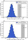 |
Fig. 15. Distribution of T bias in the RLT (top) and RYT (bottom) regions for one million simulated samples. The vertical black dashed line indicates the T bias needed to account for the results of M21 (ΔTLT and ΔTYT), and the shaded region represents its 1σ uncertainties. The p-value displayed next to it shows the probability of obtaining samples with a higher T bias than ΔTLT and ΔTYT, respectively. |
The probability that the observed LX − T and YSZ − T anisotropies in M21 are caused by an overestimation of T is 2.2 × 10⁻⁵ (4.24σ) and < 10−6 (> 4.89σ) respectively. The presence of a T decrease in our work – albeit non-significant – strongly disfavours a T bias as the cause of the M21 observed anisotropies.
7.1.2. Joint result of cosmic anisotropy with M21
The M21 study found a (9.0 ± 1.7)% angular variation in H0 in the direction of (l, b) = (280 − 35°° + 35°,−15 − 20°° + 20°). There is a strong agreement in the direction of maximum anisotropy between these findings and the results from LX − σv and YSZ − σv analysis. One of the main distinctions between the two studies is the (27.6 ± 4.4)% angular variation in H0 from the joint analysis in this work, which is significantly higher than the variation found by M21 due to a large scatter.
We performed a joint analysis with the results of M21 by pairing the datasets that are completely independent, i.e. pairing LX − σv and YSZ − σv with M21’s YSZ − T and LX − T respectively. By multiplying the posteriors of H0 for both relations, we create maps showing the H0 angular variation and its nominal significance (see Fig. 16). The maximum H0 angular variation decreased to ∼11% in both joint results, which is similar to the results of M21. The maximum nominal significance in the joint analysis of LX − σv and YSZ − T remains the same when compared to the results of LX − σv analysis. However, there is a decrease in nominal significance in the joint analysis of other relations when compared to the results of YSZ − σv analysis. A common trend in both maps is that the results of M21 dominate them due to having a low scatter in relations compared to our results.
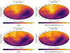 |
Fig. 16. Map of H0 angular variations (left) and its nominal significance (right) for the joint analysis of relations LX − σv & YSZ − T (top) and YSZ − σv & LX − T (bottom). |
We also checked for any correlation between the residuals of the two relations that are being used in the joint analysis. We do not find any correlation between the LX − σv and YSZ − T relations. We can, therefore, treat the two relations as independent while analysing their joint results. However, we find a correlation of ρ = −0.66 between the residuals of the YSZ − σv and LX − T relations. Thus, the joint result of these relations could underestimate the nominal significance.
7.2. Isotropic samples based on random cluster positions
Aside from using isotropic MC samples, we employed a commonly used method for generating isotropic samples, which involves shuffling the cluster positions randomly and calculating the probability of obtaining higher anisotropy in these samples compared to the observed data.
This is also known as the “look elsewhere” effect test. We created 1000 such isotropic samples for both the relations, found their maximum nominal significance values, and compared their distributions to the observed data (see Fig. 17). Our results indicate that the probability of observing higher nominal significance in an isotropic sample (based on random cluster positions) compared to the real data for the LX − σv and YSZ − σv relations are ∼5% and ∼1% respectively.
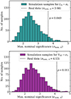 |
Fig. 17. Distribution of maximum nominal significance obtained from the 1000 isotropic samples created from the random shuffling of cluster positions for the LX − σv (top), and YSZ − σv (bottom) relations. The dashed line represents the maximum nominal significance obtained in the observed data, and the p-value next to it shows the probability of obtaining higher nominal significance than the observed data. |
When we compare these to the isotropic MC simulation results in Sect. 6.4, we find that the probability remains unchanged for the YSZ − σv relation. However, for the LX − σv relation, we note an increase in the p-value compared to isotropic MC simulation results. This decrease in significance can be attributed to our use of large cone sizes for the analysis. When we shuffle the cluster positions, it is likely that, at times, the clusters affected by the anisotropy might fall within the same cone or close to one another. As a result, the mock sample exhibits higher significance variations.
7.3. Effects of best-fit slope variations
For all three relations, we treated the slope as a free parameter, and we found some variations in best-fit slopes across the sky (see Fig. 4 for σv − T and Appendix C for LX − σv and YSZ − T). We do not expect a significant correlation between the best-fit parameters because the pivot points are chosen close to the data median. However, some cones may have a strong correlation that could bias the observed results.
To examine this, we calculated the correlation between A and B in each region and created a 2D map based on this (Fig. 18). For σv − T, the correlation between the best-fit parameters in all the regions is less than ±0.4. Similar results are also found for the YSZ − σv relation. In the analysis of LX − σv, we observe certain regions with a moderate correlation of +0.5, but these regions are distant from the anisotropy region, so we don’t have any reason to suspect a bias due to parameter correlation.
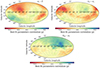 |
Fig. 18. 2D Maps of the correlation coefficient between the best-fit parameters for the σv − T (top left), LX − σv (top right), and YSZ − σv (bottom) relations. All maps have the same colour scale (−0.5 to +0.5). |
We tested our findings with the slope fixed to that of the full data to see the impact of the slight correlation between parameters (refer to Appendix C for more details). We find no significant difference in the results when the slope is fixed as compared to the free slope analysis.
7.4. Anisotropy at different z scales and with different z evolutions
We examined the distribution of redshift across different regions of the sky. If any region shows significantly higher or lower average redshift (z) values, it could indicate that we are comparing different scales, which is not ideal. It would also mean that any bias in the applied redshift evolution correction would not equally cancel out between regions. We created the redshift distribution for clusters present in the region of maximum anisotropy and compared it with the rest of the sky for the LX − σv and YSZ − σv relations (see Fig. E.1). We find that, on average, the region with maximum anisotropy has lower z, whereas the rest of the sky has a large population of clusters at higher z. Nevertheless, the distributions are overall highly similar. Even so, to ensure that our results are not biased by the population of clusters at slightly different z scales, we performed two tests. We applied various z cuts and compared these results with our initial findings, and we tested the effect of incorrect redshift evolution.
We applied several lower cuts on z, such as z > 0.03, z > 0.05, and z > 0.07 and an uppercut of z < 0.15 to our data individually and repeated our analysis. The clusters at low z are more affected by peculiar velocities; therefore, excluding them allows for a more robust comparison of underlying H0 values. Redshift cuts higher than z > 0.07 are not considered since we are limited by the number of clusters in different cones. The LX − σv relation has fewer clusters, and several cones for the cut of z > 0.07 had fewer than 20 clusters, and thus, we did not include this cut for the relation.
We plotted the positions and amplitude of regions with maximum anisotropy obtained from these cuts for both relations, including the results obtained with the full dataset in Fig. 19. These cuts return consistent results with the full sample, and we see that our results are not strongly biased due to cluster populations at different z scales. Along with these results, we also plotted the results with different z evolution power (γ).
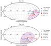 |
Fig. 19. Positions and amplitude of maximum anisotropy detected for several z cuts and z evolution power for LX − σv (top), and YSZ − σv (bottom) relations. The shaded regions represent the directional uncertainties of the full sample. |
We observe some trends in the 2D map of average z within each cone, with the northern galactic sky showing clusters at higher z compared to the southern half (see Fig. E.2). A similar galactic north-south divide is also present in the 2D maps of both relations (see Fig. 7 and Fig. 10) due to the northern galactic sky having higher A compared to the southern half. Regions with higher average z are strongly affected by incorrect redshift evolution assumptions. Therefore, it is crucial to test if the assumed γ for the two relations results in a bias and the observed galactic north-south divide in our nominal significance maps. As mentioned in the Table 1, γ for the LX − σv and YSZ − σv relations are −1 and +1 respectively. We changed γ to −2 and +2, respectively, to see the effect of choosing a strong redshift evolution on the anisotropy detected.
The results for LX − σv indicate almost no difference in nominal significance and in the direction of anisotropy. In the YSZ − σv relations, we observe minor differences from γ = +1 due to clusters with higher z in the data sample. Even when we consider the most extreme value of γ for the two relations (−10 and +10, respectively), we are unable to eliminate the north-south divide in the nominal significance maps. Therefore, we can conclude that our results are not biased due to incorrect z evolution.
8. Summary
In this work, we investigated the isotropy of the local universe using galaxy cluster scaling relations between cosmology-dependent cluster properties and a cosmology-independent property. We utilised a cosmology-independent variable that has not been used before: the velocity dispersion of a galaxy cluster. Previous studies by M21 used cluster T as their cosmology-independent quantity and found an apparent angular variation of approximately 9% in the Hubble constant, H0, across the sky.
We examined the σv − T relation across the sky to check if a position-dependent systematic bias of T measurements causes an overestimation of apparent H0 variations in the work of M21. We obtain no significant anisotropies across the sky in the σv − T relation. The probability of obtaining the observed variations for σv − T relation in an isotropic Universe is 0.72. The region with the most variations in σv − T relation is found in a similar direction as M21 but with a T underestimation of (16.3 ± 7.1)%, hinting at the possibility that the significance of the M21 results might even be underestimated. A positive T bias needed to explain the results of M21 can be rejected at a high probability (p ∼ 10−5).
We utilised the LX − σv and the YSZ − σv relations to probe the (an)isotropy of the universe. From the joint analysis, we find the most anisotropic region in the direction of (295 ° ±71 ° , − 30 ° ±71 ° ) at 3.64σ. The statistical significance is obtained using the isotropic Monte Carlo simulations. The direction of maximum anisotropy is similar to the results of M21 (l, b) = (280 − 35°° + 35°,−15 − 20°° + 20°). These results are in disagreement with the standard cosmological model. The results obtained from both these analyses further strengthen the results of M21.
The code is available at https://github.com/AdiPandya/Fast_Bayesian_Regression
Package available at https://github.com/desihub/desiutil
Acknowledgments
We thank the anonymous referee for their insightful comments and feedback that helped us improve our manuscript. L.L. acknowledges the financial contribution from the INAF grant 1.05.12.04.01.
References
- Abril-Pla, O., Andreani, V., Carroll, C., et al. 2023, PeerJ Comput. Sci., 9, e1516 [CrossRef] [Google Scholar]
- Aguado-Barahona, A., Rubiño-Martín, J. A., Ferragamo, A., et al. 2022, A&A, 659, A126 [NASA ADS] [CrossRef] [EDP Sciences] [Google Scholar]
- Andrade, U., Bengaly, C. A. P., Alcaniz, J. S., & Capozziello, S. 2019, MNRAS, 490, 4481 [Google Scholar]
- Beers, T. C., Flynn, K., & Gebhardt, K. 1990, AJ, 100, 32 [Google Scholar]
- Bennett, C. L., Kogut, A., Hinshaw, G., et al. 1994, ApJ, 436, 423 [NASA ADS] [CrossRef] [Google Scholar]
- Bennett, C. L., Larson, D., Weiland, J. L., et al. 2013, ApJ, 208, 20 [NASA ADS] [Google Scholar]
- Colin, J., Mohayaee, R., Rameez, M., & Sarkar, S. 2019, A&A, 631, L13 [NASA ADS] [CrossRef] [EDP Sciences] [Google Scholar]
- Giodini, S., Lovisari, L., Pointecouteau, E., et al. 2013, Space Sci. Rev., 177, 247 [Google Scholar]
- Girardi, M., Giuricin, G., Mardirossian, F., Mezzetti, M., & Boschin, W. 1998, ApJ, 505, 74 [NASA ADS] [CrossRef] [Google Scholar]
- Haridasu, B. S., Salucci, P., & Sharma, G. 2024, MNRAS, 532, 2234 [NASA ADS] [CrossRef] [Google Scholar]
- Hu, J. P., Wang, Y. Y., Hu, J., & Wang, F. Y. 2024, A&A, 681, A88 [NASA ADS] [CrossRef] [EDP Sciences] [Google Scholar]
- Jansen, F., Lumb, D., Altieri, B., et al. 2001, A&A, 365, L1 [NASA ADS] [CrossRef] [EDP Sciences] [Google Scholar]
- Javanmardi, B., & Kroupa, P. 2017, A&A, 597, A120 [NASA ADS] [CrossRef] [EDP Sciences] [Google Scholar]
- Kaiser, N. 1986, MNRAS, 222, 323 [Google Scholar]
- Kelly, B. C. 2007, ApJ, 665, 1489 [Google Scholar]
- Lam, S. K., Pitrou, A., & Seibert, S. 2015, Proceedings of the Second Workshop on the LLVM Compiler Infrastructure in HPC (Association for Computing Machinery), 1 [Google Scholar]
- Lopes, M., Bernui, A., Franco, C., & Avila, F. 2024, ApJ, 967, 47 [NASA ADS] [CrossRef] [Google Scholar]
- Lovisari, L., & Maughan, B. J. 2022, Handbook of X-ray and Gamma-ray Astrophysics (Springer, Singapore), 65 [Google Scholar]
- Lovisari, L., Ettori, S., Gaspari, M., & Giles, P. A. 2021, Universe, 7, 139 [NASA ADS] [CrossRef] [Google Scholar]
- Mahdavi, A., & Geller, M. J. 2001, ApJ, 554, L129 [NASA ADS] [CrossRef] [Google Scholar]
- Mazure, A., Katgert, P., den Hartog, R., et al. 1996, A&A, 310, 31 [NASA ADS] [Google Scholar]
- Mc Conville, R., Colgáin, Ó. E., 2023, Phys. Rev. D, 108, 123533 [CrossRef] [Google Scholar]
- Migkas, K. 2024, ArXiv e-prints [arXiv:2406.01752] [Google Scholar]
- Migkas, K., & Reiprich, T. H. 2018, A&A, 611, A50 [NASA ADS] [CrossRef] [EDP Sciences] [Google Scholar]
- Migkas, K., Schellenberger, G., Reiprich, T. H., et al. 2020, A&A, 636, A15 [NASA ADS] [CrossRef] [EDP Sciences] [Google Scholar]
- Migkas, K., Pacaud, F., Schellenberger, G., et al. 2021, A&A, 649, A151 [NASA ADS] [CrossRef] [EDP Sciences] [Google Scholar]
- Nagarajan, A., Pacaud, F., Sommer, M., et al. 2019, MNRAS, 488, 1728 [Google Scholar]
- Nastasi, A., Böhringer, H., Fassbender, R., et al. 2014, A&A, 564, A17 [NASA ADS] [CrossRef] [EDP Sciences] [Google Scholar]
- Ortiz-Gil, A., Guzzo, L., Schuecker, P., Böhringer, H., & Collins, C. A. 2004, MNRAS, 348, 325 [NASA ADS] [CrossRef] [Google Scholar]
- Piffaretti, R., Arnaud, M., Pratt, G. W., Pointecouteau, E., & Melin, J. B. 2011, A&A, 534, A109 [NASA ADS] [CrossRef] [EDP Sciences] [Google Scholar]
- Planck Collaboration I. 2020, A&A, 641, A1 [NASA ADS] [CrossRef] [EDP Sciences] [Google Scholar]
- Planck Collaboration VI. 2020, A&A, 641, A6 [NASA ADS] [CrossRef] [EDP Sciences] [Google Scholar]
- Planck Collaboration XXVII. 2016, A&A, 594, A27 [NASA ADS] [CrossRef] [EDP Sciences] [Google Scholar]
- Popesso, P., Biviano, A., Boehringer, H., & Romaniello, M. 2007, VizieR Online Data Catalog: J/A+A/461/397 [Google Scholar]
- Pratt, G. W., Arnaud, M., Biviano, A., et al. 2019, Space Sci. Rev., 215, 25 [Google Scholar]
- Rameez, M., Mohayaee, R., Sarkar, S., & Colin, J. 2018, MNRAS, 477, 1772 [Google Scholar]
- Reiprich, T. H., Basu, K., Ettori, S., et al. 2013, Space Sci. Rev., 177, 195 [Google Scholar]
- Rines, K. J., Geller, M. J., Diaferio, A., & Hwang, H. S. 2016, ApJ, 819, 63 [NASA ADS] [CrossRef] [Google Scholar]
- Řípa, J., & Shafieloo, A. 2017, ApJ, 851, 15 [CrossRef] [Google Scholar]
- Rubart, M., & Schwarz, D. J. 2013, A&A, 555, A117 [NASA ADS] [CrossRef] [EDP Sciences] [Google Scholar]
- Sarkar, S., Pandey, B., & Khatri, R. 2019, MNRAS, 483, 2453 [NASA ADS] [CrossRef] [Google Scholar]
- Secrest, N. J., von Hausegger, S., Rameez, M., et al. 2021, ApJ, 908, L51 [Google Scholar]
- Secrest, N. J., von Hausegger, S., Rameez, M., Mohayaee, R., & Sarkar, S. 2022, ApJ, 937, L31 [NASA ADS] [CrossRef] [Google Scholar]
- Sereno, M., & Ettori, S. 2015, VizieR Online Data Catalog: J/MNRAS/450/3675 [Google Scholar]
- Singal, A. K. 2011, ApJ, 742, L23 [NASA ADS] [CrossRef] [Google Scholar]
- Sohn, J., Geller, M. J., & Zahid, H. J. 2019, ApJ, 880, 142 [NASA ADS] [CrossRef] [Google Scholar]
- Soltis, J., Farahi, A., Huterer, D., & Liberato, C. M. 2019, Phys. Rev. Lett., 122, 091301 [Google Scholar]
- Tiwari, P., & Nusser, A. 2016, JCAP, 2016, 062 [Google Scholar]
- Voges, W., Aschenbach, B., Boller, T., et al. 1999, A&A, 349, 389 [NASA ADS] [Google Scholar]
- Wagenveld, J. D., Klöckner, H.-R., Gupta, N., et al. 2024, A&A, 690, A163 [NASA ADS] [CrossRef] [EDP Sciences] [Google Scholar]
- Weisskopf, M. C., Tananbaum, H. D., Van Speybroeck, L. P., & O’Dell, S. L. 2000, SPIE Conf. Ser., 4012, 2 [Google Scholar]
- Willingale, R., Starling, R. L. C., Beardmore, A. P., Tanvir, N. R., & O’Brien, P. T. 2013, MNRAS, 431, 394 [Google Scholar]
- Wilson, S., Hilton, M., Rooney, P. J., et al. 2016, MNRAS, 463, 413 [CrossRef] [Google Scholar]
- Xue, Y.-J., & Wu, X.-P. 2000, ApJ, 538, 65 [NASA ADS] [CrossRef] [Google Scholar]
- Yeung, S., & Chu, M. C. 2022, Phys. Rev. D, 105, 083508 [NASA ADS] [CrossRef] [Google Scholar]
- Yoon, M., Huterer, D., Gibelyou, C., Kovács, A., & Szapudi, I. 2014, MNRAS, 445, L60 [NASA ADS] [CrossRef] [Google Scholar]
- Zhai, Z., & Percival, W. J. 2022, Phys. Rev. D, 106, 103527 [NASA ADS] [CrossRef] [Google Scholar]
- Zhang, Y. Y., Andernach, H., Caretta, C. A., et al. 2011, A&A, 526, A105 [NASA ADS] [CrossRef] [EDP Sciences] [Google Scholar]
Appendix A: Choice for the cone and interval sizes
The cone size was chosen such that the number of clusters inside the cone is as large as possible without covering too large an area. Four cone sizes were considered to decide the best size for the analysis. The radii of these cones are 90°, 75°, 60°, and 45°. Fig. A.1 shows the number of clusters inside a cone for the relation σv − T for different cone sizes.
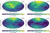 |
Fig. A.1. Maps of the number of clusters for different cone sizes in the relation σv − T. The cone sizes are 90° (top left), 75° (top right), 60° (bottom left), and 45° (bottom right). Note that the colour scale is different for the four plots. |
The cone size of 45° covers a small area, and the number of clusters inside the cone is also small. There are less than ten clusters in the region of the Galactic belt. The cone size of 90° covers a large area, and the number of clusters inside the cone is also large. This creates a significant overlap between the cones. The cone size of 60° has a high number of clusters for most regions, but certain regions have less than 20 clusters. The cone size of 75° strikes a good balance between the area covered and the number of clusters inside the cone. Thus, the cone size of 75° was chosen for the analysis.
The centre for these cones was taken at a step size of 5°. This was mainly done to reduce the computation time. Fig. A.2 shows the nominal significance of the best-fit A for the relation σv − T for different step sizes. The results show that the choice of step size does not affect the results significantly.
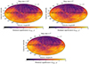 |
Fig. A.2. Nominal sigma map of the A from the σv − T relation for different step sizes. The step sizes are 10° (top left), 5° (top right), and 1° (bottom). |
In the nominal significance map with a step size of 1°, some artefacts are seen as curved lines. These artefacts can be seen in the nominal significance map with a step size of 5°, but they are not as prominent. These artefacts are due to strong outliers present in a particular region. These clusters were not considered outliers when considering the entire sample. All regions with this strong outlier will produce similar best-fit results, creating the artefacts.
Appendix B: Redshift trends in the residuals
Using the Y|X best-fit minimisation method, strong LX (and YSZ) residual trends are observed as a function of cluster redshift. Fig. B.1 shows the y-axis residuals for the relations LX − σv and YSZ − σv as a function of z using the Y|X and X|Y minimisation methods.
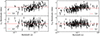 |
Fig. B.1. Y-axis residual trends with respect to cluster redshift for the LX − σv (left) and YSZ − σv (right) relations. The top panel displays the residuals using the Y|X minimisation, and the bottom panel displays the residuals using the X|Y minimisation method. |
It is generally known that when there are significant uncertainties on the x-axis while minimising on the y-axis, the best-fit results can show strong biases. Therefore, we adopted the X|Y minimisation for this scaling relation as these trends are not observed in this method.
Appendix C: Comparison between free slope and fixed slope
We observe variations in the best-fit slope in certain regions for all three relations (see Fig. 4 and Fig. C.1). Although there are no strong correlations between the best-fit parameters, additional tests are conducted by keeping the slope fixed at the value obtained from the full sample.
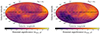 |
Fig. C.1. Nominal significance maps of best-fit B for LX − σv (left), and YSZ − σv (right) relations. |
Figure C.2 compares the free and fixed slope analysis results for all three relations. We calculated ΔσA as the difference of nominal σA obtained from the fixed and free slope analysis. For the σv − T and LX − σv relations, these differences are less than ±0.5σnom. However, for the YSZ − σv, there are somewhat higher differences (∼0.8σnom) in certain regions. Nonetheless, the direction and magnitude of the maximum nominal significance obtained for this relation remain unchanged. Therefore, we can infer that the variations in the best-fit slope are not a major concern as they do not impact the conclusions drawn from the analysis as expected, given the rather weak correlation observed between slope and normalisation.
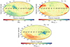 |
Fig. C.2. Difference between the nominal significance of A obtained from fixed slope and free slope analysis for the σv − T (top left), LX − σv (top right), and YSZ − σv (bottom) relations. Top panel maps have the same colour scale (−0.5 to +0.5), whereas the bottom panel map has a colour scale of −0.9 to +0.9 to visualise higher variations. |
Appendix D: General behaviour of scaling relations for different datasets and fitting methods
The Table D.1 presents the best-fit parameters for the relations LX − σv and YSZ − σv obtained using different datasets and fitting methods. The best-fit parameters are consistent across the different datasets. Notably, the X|Y fitting method consistently yields a higher slope than the Y|X minimisation method for the various datasets.
Comparison of best-fit parameters for the LX − σv and YSZ − σv scaling relations with different datasets.
Appendix E: z distributions
The Fig. E.1 shows the distribution of cluster redshift in the region of maximum anisotropy and the rest of the sky for the two relations LX − σv and YSZ − σv. We observe some differences between the distributions of the two regions. On average, clusters in the most anisotropic regions have lower z.
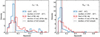 |
Fig. E.1. Distribution of redshifts for the clusters inside the cone centred at maximum anisotropy and rest of the sky for LX − σv (left), and YSZ − σv (right) relations |
We also created a 2D map of the average z within each cone to identify other z trends in our data (see Fig. E.2). This value is calculated using the same weighting scheme mentioned in the Sect. 3.3. The most significant trend observed is the galactic north-south divide for the LX − σv relation. On average, clusters are found at higher z in the northern galactic sky compared to the southern half.
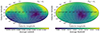 |
Fig. E.2. 2D map of average redshifts of the clusters inside a cone for LX − σv (left), and YSZ − σv (right) relations. |
Appendix F: Relation between A and H0
The best-fit normalisation is related to the Hubble parameter, and variations in the best-fit normalisation can be converted to variations in the Hubble parameter. For the relation LX − σv (LX = A × σvB),

Here, fX is the observed X-ray flux, Kcorr is the K correction used to convert LX from the rest frame of the observer to the cluster’s rest frame, and DL(z) is the luminosity distance, which is given by
Thus, the equation becomes
This is also true for the YSZ − σv relation since the quantity YSZ depends on the integrated Compton parameter Y and square of the angular diameter distance (DA(z)). Thus, the equation YSZ = A × σvB transforms to
This shows that absolute constraints can only be put on the quantity H02A. To obtain the value of H0 in different regions of the sky from A, equation 6 is used.
All Tables
Maximum anisotropy direction and its absolute amplitude for the LX − σv and YSZ − σv relations along with absolute H0 variation.
Maximum anisotropy direction for the LX − σv and YSZ − σv relations along with H0 angular variation.
Comparison of best-fit parameters for the LX − σv and YSZ − σv scaling relations with different datasets.
All Figures
|
Fig. 1. Sky distribution of the galaxy clusters used in the scaling relations σv − T (left), LX − σv (middle), and YSZ − σv (right). The clusters’ redshifts are colour-coded. |
| In the text | |
|
Fig. 2. Example of a region used for two-dimensional scanning centred at (l, b) = (60 ° ,15 ° ) with cone size, θ, of radius 75° for σv − T relation. Different colours represent the statistical weights assigned to the clusters inside these regions. ∑ represents the number of clusters inside this region. |
| In the text | |
|
Fig. 3. Best-fit plots for the three scaling relation. The shaded regions represent 1σ uncertainties of the best-fit parameters. From left to right:σv − T (Y|X), LX − σv (X|Y), and YSZ − σv (X|Y) relations. |
| In the text | |
|
Fig. 4. Left panel: maps of best-fit normalisation (top) and the slope (bottom) compared to the full sample for the σv − T relation. Note that the colour scale is different for both maps. This highlights the small variations in the A/Aall map. Right panel: nominal significance maps for the normalisation (top) and slope (bottom). Both maps have the same colour scale (−3σnom to +3σnom). A negative sigma value refers to a value lower than the rest of the sky. |
| In the text | |
|
Fig. 5. Map of percentage T bias between a region and rest of the sky. Negative T variations refer to an underestimation of T compared to the rest of the sky. To alleviate the observed anisotropies in M21, the behaviour required would have to be opposite to what is observed. |
| In the text | |
|
Fig. 6. Distribution of maximum nominal sigma values and its %T bias obtained from the 1000 isotropic Monte Carlo simulated samples of the σv − T relation. Shaded contours represent 68%, 95%, and 99% confidence levels. The value obtained in the real data is shown by a black dashed line on the histograms and by a point on the contour plot. The p-value in the histogram of maximum nominal sigma values represents the probability of getting higher nominal significance than the real data. |
| In the text | |
|
Fig. 7. Map of best-fit A compared to the full sample (left) and its nominal significance map (right) for the LX − σv relation. |
| In the text | |
|
Fig. 8. H0 angular variation map created from the LX − σv relation. |
| In the text | |
|
Fig. 9. Distribution of H0 values corresponding to each data point in the region of maximum anisotropy and rest of the sky for the relations LX − σv (top) and YSZ − σv (bottom). The median of both distributions is shown by dashed lines along with H0 = 70 km s−1 Mpc−1. Note that both regions have different numbers of clusters, and thus, to compare both, the density of the distribution is plotted. |
| In the text | |
|
Fig. 10. Map of best-fit A compared to the full sample (left) and its nominal significance map (right) for the YSZ − σv relation. Both maps have the same colour scale as Fig. 7. |
| In the text | |
|
Fig. 11. H0 angular variation map created from the YSZ − σv relation. The map has the same colour scale as Fig. 8. |
| In the text | |
|
Fig. 12. Correlation between the residuals of the relations LX − σv and YSZ − σv. The best-fit line is shown in orange, along with the correlation coefficient. |
| In the text | |
|
Fig. 13. H0 angular variation maps created from the joint analysis of relations LX − σv and YSZ − σv (top) and its nominal significance map (bottom). Colour scales for the H0 angular variation map are the same as before, but the colour scales for the sigma map have been increased to account for increased significance. |
| In the text | |
|
Fig. 14. Distribution of maximum nominal sigma values and its ΔH0 variations obtained from the 1000 isotropic Monte Carlo simulated samples of the LX − σv (left) and YSZ − σv (right) relations. Shaded contours represent 68%, 95%, and 99% confidence levels. The value obtained in the real data is shown by a black dashed line on the histograms and by a point on the contour plot. The p-value in the histogram of maximum nominal sigma values represents the probability of getting higher nominal significance than the real data. |
| In the text | |
|
Fig. 15. Distribution of T bias in the RLT (top) and RYT (bottom) regions for one million simulated samples. The vertical black dashed line indicates the T bias needed to account for the results of M21 (ΔTLT and ΔTYT), and the shaded region represents its 1σ uncertainties. The p-value displayed next to it shows the probability of obtaining samples with a higher T bias than ΔTLT and ΔTYT, respectively. |
| In the text | |
|
Fig. 16. Map of H0 angular variations (left) and its nominal significance (right) for the joint analysis of relations LX − σv & YSZ − T (top) and YSZ − σv & LX − T (bottom). |
| In the text | |
|
Fig. 17. Distribution of maximum nominal significance obtained from the 1000 isotropic samples created from the random shuffling of cluster positions for the LX − σv (top), and YSZ − σv (bottom) relations. The dashed line represents the maximum nominal significance obtained in the observed data, and the p-value next to it shows the probability of obtaining higher nominal significance than the observed data. |
| In the text | |
|
Fig. 18. 2D Maps of the correlation coefficient between the best-fit parameters for the σv − T (top left), LX − σv (top right), and YSZ − σv (bottom) relations. All maps have the same colour scale (−0.5 to +0.5). |
| In the text | |
|
Fig. 19. Positions and amplitude of maximum anisotropy detected for several z cuts and z evolution power for LX − σv (top), and YSZ − σv (bottom) relations. The shaded regions represent the directional uncertainties of the full sample. |
| In the text | |
|
Fig. A.1. Maps of the number of clusters for different cone sizes in the relation σv − T. The cone sizes are 90° (top left), 75° (top right), 60° (bottom left), and 45° (bottom right). Note that the colour scale is different for the four plots. |
| In the text | |
|
Fig. A.2. Nominal sigma map of the A from the σv − T relation for different step sizes. The step sizes are 10° (top left), 5° (top right), and 1° (bottom). |
| In the text | |
|
Fig. B.1. Y-axis residual trends with respect to cluster redshift for the LX − σv (left) and YSZ − σv (right) relations. The top panel displays the residuals using the Y|X minimisation, and the bottom panel displays the residuals using the X|Y minimisation method. |
| In the text | |
|
Fig. C.1. Nominal significance maps of best-fit B for LX − σv (left), and YSZ − σv (right) relations. |
| In the text | |
|
Fig. C.2. Difference between the nominal significance of A obtained from fixed slope and free slope analysis for the σv − T (top left), LX − σv (top right), and YSZ − σv (bottom) relations. Top panel maps have the same colour scale (−0.5 to +0.5), whereas the bottom panel map has a colour scale of −0.9 to +0.9 to visualise higher variations. |
| In the text | |
|
Fig. E.1. Distribution of redshifts for the clusters inside the cone centred at maximum anisotropy and rest of the sky for LX − σv (left), and YSZ − σv (right) relations |
| In the text | |
|
Fig. E.2. 2D map of average redshifts of the clusters inside a cone for LX − σv (left), and YSZ − σv (right) relations. |
| In the text | |
Current usage metrics show cumulative count of Article Views (full-text article views including HTML views, PDF and ePub downloads, according to the available data) and Abstracts Views on Vision4Press platform.
Data correspond to usage on the plateform after 2015. The current usage metrics is available 48-96 hours after online publication and is updated daily on week days.
Initial download of the metrics may take a while.