| Issue |
A&A
Volume 691, November 2024
|
|
|---|---|---|
| Article Number | A124 | |
| Number of page(s) | 18 | |
| Section | Extragalactic astronomy | |
| DOI | https://doi.org/10.1051/0004-6361/202451738 | |
| Published online | 05 November 2024 | |
Mapping AGN winds: A connection between radio-mode AGNs and the AGN feedback cycle
1
Zentrum für Astronomie der Universität Heidelberg, Astronomisches Rechen-Institut, Mönchhofstr, 12-14, 69120 Heidelberg, Germany
2
University of Colorado Boulder, 2000 Colorado Avenue, Boulder, CO 80309, USA
3
Department of Astrophysical Sciences, Princeton University, 4 Ivy Lane, Princeton, NJ 08544, USA
4
Departamento de Física, Centro de Ciências Naturais e Exatas, Universidade Federal de Santa Maria, 97105-900 Santa Maria, RS, Brazil
5
Laboratorio Interinstitucional de e-Astronomia – LIneA, Rua Gal. José Cristino 77, Rio de Janeiro, RJ 20921-400, Brazil
⋆ Corresponding author; malban@uni-heidelberg.de
Received:
31
July
2024
Accepted:
27
August
2024
We present a kinematic analysis based on the large integral field spectroscopy (IFS) dataset of SDSS-IV MaNGA (Sloan Digital Sky Survey/Mapping Nearby Galaxies at Apache Point Observatory; ∼10 000 galaxies). We have compiled a diverse sample of 594 unique active galactic nuclei (AGNs), identified through a variety of independent selection techniques, encompassing radio (1.4 GHz) observations, optical emission-line diagnostics (BPT), broad Balmer emission lines, mid-infrared colors, and hard X-ray emission. We investigated how ionized gas kinematics behave in these different AGN populations through stacked radial profiles of the [O III] 5007 emission-line width across each AGN population. We contrasted AGN populations against each other (and non-AGN galaxies) by matching samples by stellar mass, [O III] 5007 luminosity, morphology, and redshift. We find similar kinematics between AGNs selected by BPT diagnostics compared to broad-line-selected AGNs. We also identify a population of non-AGNs with similar radial profiles as AGNs, indicative of the presence of remnant outflows (or fossil outflows) of past AGN activity. We find that purely radio-selected AGNs display enhanced ionized gas line widths across all radii. This suggests that our radio-selection technique is sensitive to a population in which AGN-driven kinematic perturbations have been active for longer durations (potentially due to recurrent activity) than in purely optically selected AGNs. This connection between radio activity and extended ionized gas outflow signatures is consistent with recent evidence that suggests radio emission (expected to be diffuse) originated due to shocks from outflows. We conclude that different selection techniques can trace different AGN populations not only in terms of energetics but also in terms of AGN evolutionary stages. Our results are important in the context of the AGN duty cycle and highlight integral field unit data’s potential to deepen our knowledge of AGNs and galaxy evolution.
Key words: galaxies: active / galaxies: evolution / quasars: supermassive black holes
© The Authors 2024
 Open Access article, published by EDP Sciences, under the terms of the Creative Commons Attribution License (https://creativecommons.org/licenses/by/4.0), which permits unrestricted use, distribution, and reproduction in any medium, provided the original work is properly cited.
This article is published in open access under the Subscribe to Open model. Subscribe to A&A to support open access publication.
1. Introduction
Active galactic nuclei (AGNs) have become a common element in galaxy evolution studies (Heckman & Best 2014) and a fundamental engine for supermassive black hole (SMBH) growth (Alexander & Hickox 2012). Observational studies have suggested the connection between SMBHs and their host galaxies, finding significant empirical correlations between them (Kormendy & Ho 2013). Specifically, the mass of the SMBH has been seen to correlate with fundamental galaxy properties such as the bulge luminosity (Ferrarese & Merritt 2000) and the bulge velocity dispersion (Marconi & Hunt 2003). Further evidence has shown that the star formation rate history in galaxies peaks at z ∼ 2, exactly where the black hole accretion history (related to AGN activity) is at its height (Madau & Dickinson 2014; Aird et al. 2015). This suggests an interaction (and coevolution) between the AGN and the interstellar medium (ISM) of its host galaxy (Fabian 2012; Morganti 2017b), known as AGN feedback. Indeed, the released energy required for such a massive black hole to have grown is comparable to or greater than the binding energy of the host galaxy itself (Silk & Rees 1998), placing AGNs in the spotlight as relevant for understanding galaxy evolution (see also Hopkins et al. 2006).
A common property of galaxies hosting an AGN is the presence of strong winds or outflows (e.g., Mullaney et al. 2013; Harrison et al. 2014; Cheung et al. 2016; Wylezalek et al. 2020) in the ionized gas. Such outflows can be deployed in the form of collimated jets (Worrall & Birkinshaw 2006) or as radiatively driven winds (Netzer 2006) where gas can be ejected and transferred into the host galaxy (see King & Pounds 2015, for a review). This ubiquitous characteristic is a popular mechanism to explain how AGN feedback works and has been a key parameter introduced to solve theoretical problems faced in cosmological simulations (Somerville & Davé 2015; Naab & Ostriker 2017). For example, one notable application is helping to explain the regulation of star formation in massive galaxies (see also Harrison 2017). These phenomena (winds or outflows) have been observed in multiple gas phases (e.g., Aalto et al. 2012; Fiore et al. 2017; Herrera-Camus et al. 2020; Baron et al. 2021; Riffel et al. 2023), from extremely broad X-ray outflow features (reaching fractions of the speed of light; Tombesi et al. 2012) to cold-molecular gas winds (e.g., Cicone et al. 2014).
Even when focusing on one specific phase, outflow signatures can turn out to be very complex (e.g., Zakamska et al. 2016a). In the ionized gas (the main subject of this paper), for example, such outflows display nongravitational winds with a velocity dispersion (full width at half maximum (FWHM) > 500 km s−1) that cannot be explained by the intrinsic rotation of the host galaxy or its dynamical equilibrium (Karouzos et al. 2016). Outflows usually appear in the spectra as secondary spectral components that accompany the main spectral lines (e.g., Heckman et al. 1981; Mullaney et al. 2013). Therefore, the shape of these spectral lines can acquire complex features that a single Gaussian profile cannot model. Instead, multicomponent fitting procedures have been widely used to characterize outflow signatures (e.g., Förster Schreiber et al. 2014). A widely used tracer to study these signatures is the [O III]λ5007 emission line. This forbidden emission line is restricted to low-density environments (such as the narrow-line region) and can be produced as a result of shocks or photoionization (Osterbrock 1989).
Much of what has been learned from AGNs has been through the study of their ionized gas kinematics. For example, in a large sample of optically selected type II AGNs, Woo et al. (2016) found that the velocity dispersion of the outflow as well as the fraction of emission-line ([O III]) shapes exhibiting multiple components both tend to escalate with an increase in [O III] luminosity (L[O III]). This is relevant because the L[O III] has been shown to be a good indicator of an AGN’s bolometric luminosity (Lbol; Heckman et al. 2004; LaMassa et al. 2010), which is an important parameter to understand the involved energy injection of the AGN’s SMBH (Heckman & Best 2014) to the host galaxy. For example, Fiore et al. (2017) found that the wind mass outflow rate correlates with Lbol.
Ionized outflows have been routinely found in AGNs selected from infrared (e.g., DiPompeo et al. 2018), X-ray (e.g., Rojas et al. 2019) and optical surveys (e.g., Wylezalek et al. 2020), to mention a few examples. However, none of the multiple AGN selection techniques today offer an ultimately clean AGN population (Padovani 2017) by itself. Attempts to create more complete AGN samples have shown that different selection techniques can find AGN candidates that other single selection techniques would miss (e.g., Alberts et al. 2020). Statistical analysis of AGNs selected based on techniques that are limited to a certain wavelength window can suffer from important biases such as obscuration or data coverage. This is not a simple task and different selection techniques (using various wavelengths) find different AGN populations, even with contrasting host-galaxy properties (e.g., Hickox et al. 2009; Comerford et al. 2020; Ji et al. 2022).
Consequently, the estimated outflow properties, and therefore AGN feedback studies, can be compromised by the way the AGN population is selected. For example, Mullaney et al. (2013) found that the most extreme [O III] kinematics arise from AGNs with moderate radio luminosities (1023 W Hz−1 > L1.4 GHz > 1025 W Hz−1), finding evidence of compact radio cores being responsible for driving the most broadened profiles (see also Jarvis et al. 2019, 2021; Molyneux et al. 2019). Baron & Netzer (2019) found that AGNs that present outflows (using the [O III] emission line) exhibit an excess in the mid-infrared spectral energy distribution component, suggesting that outflows are carrying dust. Different selection techniques can also be sensitive to different AGN powering mechanisms or stages of the current AGN duty cycle. The latter has been suggested by directly comparing optically selected AGN candidates with mid-infrared radio-detected AGN candidates (see Kauffmann 2018), with the former being found to dominate black hole growth in lower-mass systems.
An additional complication is that ionized outflows can extend from sub-kiloparsec (e.g. Singha et al. 2022) to kiloparsec scales (e.g., Liu et al. 2010; Sun et al. 2017). Due to the limitations of the instruments, most of the studies mentioned above base their results on single-fiber observations. Integral field spectroscopy (IFS) is a valuable technique to study the spatial distribution of outflows in more detail (e.g., Wylezalek et al. 2018; Luo et al. 2021; Singha et al. 2022). One of the latest pioneering IFS surveys is the MaNGA (Mapping Nearby Galaxies at Apache Point Observatory) survey (Bundy et al. 2015), providing 10 010 unique galaxies with spatially resolved spectra. Hence, our primary objective is to investigate how outflow properties vary, not only spatially but also based on the selection technique employed. The responsiveness of our selection methods to outflow characteristics can potentially shed light on their driving mechanisms and a connection to the AGN duty cycle.
This paper is organized as follows. In Sect. 2, we describe our data and some available catalogs for them that are relevant to this study to assemble a multiwavelength AGN catalog. The methods employed to study our sample are described in Sect. 3, with a description of the host galaxy properties of our sample. The results are explained in Sect. 4, and we present a discussion in Sect. 5. Lastly, we summarize our conclusions in Sect. 6. The cosmological assumptions used in this study are H0 = 72 km s−1 Mpc−1, ΩM = 0.3, and ΩΛ = 0.7.
2. Sample and catalogs
2.1. The MaNGA Survey
In this study, we have used the ∼10 000 galaxies (0.01 < z < 0.15) observed in the SDSS-IV/MaNGA survey (Sloan Digital Sky Survey/Mapping Nearby Galaxies at Apache Point Observatory). MaNGA is an integral field unit (IFU) survey, providing 2D mapping of optical spectra at 3622–10 354 Å at a resolution of R ∼ 2000. Its field of view ranges from 12″ to 32″ in diameter. Data reduction has been performed by MaNGA’s Data Reduction Pipeline (DRP, Law et al. 2015). Complete spectral fitting is provided by MaNGA’s data analysis pipeline (DAP, Westfall et al. 2019). The DAP fits models for multiple spectral components (e.g., stellar continuum, emission lines) to the entire spectra. Throughout this paper, we have used the spectra (reduced by the DRP) after subtracting their stellar continuum (i.e., emission-line-only spectra provided by the DAP; see details in Sect. 3).
Additionally, Sánchez et al. (2022) presents a comprehensive catalog reporting multiple characteristics and integrated host galaxy properties based on a full spectral analysis with the pyPipe3D pipeline (Lacerda et al. 2022). Most of the galaxy properties used in our study are taken from this catalog (e.g., stellar mass and star formation rates). Other galaxy properties, such as emission-line ratios and Hα equivalent widths (EW(Hα)), are taken from (Albán & Wylezalek 2023). In this paper, we furthermore compute additional parameters, as is described in Sect. 3 (e.g., L[O III]).
2.2. Active galactic nucleus catalogs
This paper aims to assess the behavior of spatially resolved ionized gas kinematics in AGN samples selected through various selection methods1. We have used the following set of MaNGA-AGN catalogs, which we shall further describe in subsequent subsections:
-
An optical emission-line-based catalog from Albán & Wylezalek (2023) (using the 2 kpc aperture).
-
A broad-line-based AGN catalog from Fu et al. (2023).
-
A mid-infrared-selected AGN catalog from Comerford et al. (2024).
-
A hard X-ray-selected AGN catalog from Comerford et al. (2024).
-
A catalog of radio-selected AGNs that we construct in this paper (see Sect. 2.2.4).
The full MaNGA sample contains a small number of repeated observations, most of which can be identified through their MaNGA-IDs (although there are exceptions; see more in Appendix A). We exclude duplicate sources in our final statistics, tables, and figures. In the following sections, we describe the individual AGN catalogs and the respective selection criteria in more detail. The sky coverage of the different surveys used for the classifications described below overlaps with MaNGA.
2.2.1. DR17 optical AGN catalog in flexible apertures from Albán & Wylezalek
Albán & Wylezalek (2023) present galaxy classifications based on optical emission-line diagnostics (Baldwin et al. 1981; Veilleux & Osterbrock 1987) measured within apertures of varying size for the entire MaNGA survey. Galaxies are classified into star-forming (SF), composite, Seyfert, LINER (low-ionization emission-line region, Halpern & Steiner 1983), or ambiguous galaxies (e.g., if a galaxy received two different classifications based on different line ratio diagnostics). The final AGN sample is then defined based on the galaxies in the Seyfert and LINER classes, with an additional cut on Hα equivalent width > 3 Å2 This additional cut minimized the contamination of faint “fake” AGNs (Cid Fernandes et al. 2010).
In this paper, we have used the 399 AGN candidates from the catalog based on a 2 kpc aperture3. The aperture was chosen to keep a balance between MaNGA’s spatial resolution limit (∼1.37 kpc, Wake et al. 2017) and the physical extent of gas ionized by an AGN (known as the narrow-line region (NLR), Bennert et al. 2006; Netzer 2015).
2.2.2. Broad-line AGN catalog
Some active galaxies present broad Balmer emission lines (known as type I AGNs; e.g., Oh et al. 2015). This is attributed to Doppler broadening due to high-velocity ionized gas surrounding the SMBH (Peterson 2006). Comerford et al. (2020) have presented a crossmatch between the MaNGA survey and Oh et al. (2015)’s type I classification that is based on SDSS DR7 data single-fiber spectroscopic observations with a size of 3″. More recently, Fu et al. (2023) has carried out an analysis to identify broad-line AGNs and double-peaked emission-line signatures for the total MaNGA sample using the DR17 data release. MaNGA not only uses smaller fibers (2″) but also provides additional spatial information.
For each galaxy, Fu et al. (2023) used DAP flux residuals to compare them to the original flux in specific spectral regions (with a size of 20 Å) corresponding to the location of Hα and [O III] emission lines to assess the quality of the DAP’s fitting procedure. They arranged the sample in 20 S/N bins (G-band S/N from the DAP) and selected galaxies with residuals > 1σ of the residual distribution at each S/N bin (see details on Fu et al. 2023). They then performed a spectral fitting on this sample of 1652 galaxies, allowing multiple components to be fit to emission lines.
They ultimately selected broad-line AGNs as galaxies where the emission-line width (σ) of the broad component is at least 600 km s−1 larger than the emission-line width of the narrow component and present a catalog of 139 broad-line AGN (type I) candidates. We have found a few duplicate galaxies in this catalog’s observations (see Appendix A), which reduces the sample to 135 targets. The work by Fu et al. (2023) almost doubles the number of broad-line-selected galaxies presented Comerford et al. (2020); on the other hand, 21 galaxies presented in Comerford et al. (2020) are not found in Fu et al. (2023). Discrepancies in the latter context can be related to the difference in FWHM(Hα) constraints and possibly effects from changing-look AGNs (see Ricci & Trakhtenbrot 2023, for a review).
2.2.3. Mid-infrared and X-ray AGN catalogs of Comerford et al.
Comerford et al. (2024) have crossmatched MaNGA galaxies with known AGN candidates from multiwavelength surveys (as in Comerford et al. 2020). In this study, we have used the following catalogs:
-
Mid-infrared AGN catalog based on observations with the Wide-field Infrared Survey Explorer (Wright et al. 2010, WISE): 123 AGNs.
-
X-ray-selected catalog based on observations with the Burst Alert Telescope (Barthelmy et al. 2005, BAT): 29 AGNs.
Comerford et al. (2024) also provide a radio-AGN catalog and a broad-line (type I) AGN catalog, which we hae chosen not to use due to our science goals (see Sects. 2.2.4 and 2.2.2, respectively). Due to repeated observations or critical flags (from the MaNGA DRP; see the details in Appendix A), we excluded seven galaxies from the mid-infrared-selected catalog (three were repeated) and one from the X-ray-selected one (one has a critical flag).
2.2.4. Selection of radio AGNs
In this section, we present a catalog of AGN candidates solely based on radio data and independent of the radio-loud or radio-quiet classification often used in the literature. They were chosen independently of whether or not they have a jet (see the details in some comprehensive reviews; e.g., Heckman & Best 2014; Padovani 2016; Panessa et al. 2019). For example, Best & Heckman (2012) used a selection technique combining both optical and radio signatures, and this is the catalog that Comerford et al. (2024) presents as the radio-selected MaNGA AGN population (see Sect. 2.2.3). However, this classification prioritizes sources with f1.4 GHz > 5 mJy as its emphasis lies on the radio-loud population of AGNs (see Urry & Padovani 1995; Padovani et al. 2017, for a review). Instead, we used a different approach and first crossmatched MaNGA SDSS-IV galaxies with data from the NRAO Very Large Array Sky Survey (Condon et al. 1998, NVSS) and the Faint Images of the Radio Sky at Twenty centimeters (Becker et al. 1995, FIRST) radio surveys, adopting a less strict flux cut of > 1 mJy. We note that this threshold is close to the sensitivity of the surveys, and there is likely a population of AGNs emitting even below this limit (e.g., White et al. 2015).
Previous studies have shown that finding genuine associations between targets of two different surveys comes with a trade-off between completeness and reliability (e.g., Best et al. 2005; Ivezić et al. 2002). Choosing a larger offset for searching counterparts can lead to high completeness but increases the number of false associations. To ensure precise spatial alignment between the optical and radio sources, we searched for the closest galaxy within a 1.5 arcsecond aperture for the FIRST survey, which ensures 85% completeness and 97% reliability (see Ivezić et al. 2002), and we used a 5.0 arcsecond aperture for the NVSS survey. For comparison, Best et al. (2005) estimates 90% completeness and 6% contamination from random targets using a 10.0 arcsecond aperture. This choice of apertures aims to maximize completeness and reliability. We find 936 and 1035 crossmatches for the FIRST and NVSS survey, respectively. In total, 1383 unique targets were found, with 588 coincident targets between FIRST and NVSS.
Our aim is to develop a radio-selected sample that is as independent as possible of known optical diagnostics (e.g., BPT diagrams) or other selection criteria. Two significant contributors to the extragalactic radio sky are star formation processes and nuclear activity in galaxies (Padovani 2016). The host galaxies of AGNs have been shown to span several decades in radio luminosity, and are often very faint, raising the question of whether their radio emission is dominated by star formation processes (Panessa et al. 2019) rather than the AGN event. Zakamska et al. (2016b) studied whether the radio signatures (1.4 GHz flux density) of confirmed AGNs can be explained purely by star formation processes when comparing them with a variety of star formation rate tracers. Independently of the used SFR tracer, they conclude that the AGNs had a systematic excess in radio luminosity not consistent with star formation, which might be attributed to the activity in the nucleus. Similarly, Kauffmann et al. (2008) used the Hα luminosity and compared it with the 1.4 GHz flux densities of a sample of SDSS galaxies (crossmatched with radio surveys; FIRST and NVSS) and found that SF galaxies form a tight correlation between both parameters and that their AGN candidates systematically exceed this tight relation toward higher 1.4 GHz flux densities.
Based on the findings described above, we constructed a radio-selected AGN sample similar to the “LHα versus Lrad” method used in Best & Heckman (2012). Specifically, we identified AGN activity based on the excess in the SFR estimated from the radio luminosity compared to the Hα-based SFR reported in the PIPE3D value-added catalog of Sánchez et al. (2022); that is, values that are above the expected 1-to-1 relation. We used the extension named log_SFR_SF, meaning that only the spaxels that were consistent with star formation regions were used to measure the SFR. Additional ways to minimize or correct for the contribution of the AGN during the SFR measurement have been shown in De Mellos in prep. We note that different methods to estimate the SFR from optical spectra (e.g., the SSP-method, Sánchez et al. 2022) do not change our results significantly (as has also been seen in Zakamska et al. 2016b).
In Fig. 1, we show the relation between the Hα-based SFR and the radio-based SFR for the radio-detected MaNGA galaxies described above, assuming that all radio emission is related to SF processes. We also show the density contours of different galaxy subclasses based on optical diagnostics presented in Albán & Wylezalek (2023) and described in Sect. 2.2.1. Pure SF galaxies agglomerate close to the 1-to-1 line (dashed blue contours), in agreement with the findings presented in Kauffmann et al. (2008). Composite galaxies (see Sect. 2.2.1) occupy values consistent with a radio excess (solid cyan contours). Indeed, the emission in composite galaxies is expected to be a mix of star formation and AGN processes. We also show the location of AGN candidates that have been selected by any of the described selection techniques (apart from a radio selection) – that is, using mid-infrared, hard X-rays (see Sect. 2.2.3), broad lines (see Sect. 2.2.2), and optical diagnostics (see Sect. 2.2.1) – and label this sample as “AGN (no radio)” in the figure (solid teal-colored line). We show that this AGN population gathers preferentially in the excess region of the plot, consistent with the findings of Zakamska et al. (2016b) and Kauffmann et al. (2008). On the top and right-hand borders of the plot, we show the distribution of the individual SFR values using a smooth histogram.
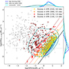 |
Fig. 1. Definition of the radio-selected AGN candidates. We plot on the y axis the expected SFR that one would measure, assuming that all the radio luminosity can be attributed to star formation processes (SFR(Lrad); see Sect. 2.2.4). Similarly, on the x axis, the SFR is expected from Hα luminosity (SFR(Hα)). The black line corresponds to the location where SFR(Lrad) = SFR(Hα). The other colored lines (orange, red, and blue) correspond to our SFR excess definition in SFR(Hα) steps of 0.5, 1.0, and 1.5 dex (log(xi)). We defined each sample of AGN-selected candidates by selecting the targets whose values (and error bars) are above the corresponding line (following SFR(Lrad)/SFR(Hα) = xi) and we have colored them according to the colored lines (except for xi = 0.0 dex, which corresponds to the yellow ones). We also show targets that did not satisfy any SFR-excess criteria (gray without marker) or did not pass the S/N criteria (gray with marker) for our kinematic analysis (see Sect. 3.2). The contours (dashed blue, light blue, and teal) represent the density where specific galaxy populations gather (SF, composite, non-radio-selected AGNs). The top and right-hand plots show the individual parameter distribution of these three galaxy populations. |
Using offsets from the 1-to-1 line, following SFR(Lrad)/SFR(Hα) = xi, we have colored with yellow, orange, red, and maroon the galaxy populations with excesses from log(xi) = 0.0 to log(xi) = 1.5 dex. The gray-colored targets in the plot represent the galaxies that we excluded from our analysis due to one or two of two reasons: they were not above the 1-to-1 relation, or their signal-to-noise (S/N) from the [O III] 5007 emission line was too low-quality to be accepted for our kinematic analysis (see Sect. 3.2).
We defined our radio-AGN sample using the galaxies whose Lrad plus associated flux uncertainties were at least 0.5 dex above the 1-to-1 SFR relation. We find 642 galaxies that satisfy this criterion, while 28 of those are either duplicate or critical targets (see Appendix A). We note that only 5% of the SF classified galaxies are above the 0.5 dex line. Employing larger cutoffs risks excluding low-luminosity AGNs. Notably, 25% of targets identified as AGNs by alternative methods – in other words, excluding radio observations – were found below the 0.5 dex line. Taking into account additional quality criteria necessary for our emission-line analysis (see Sect. 3.2), we worked with a sample of 288 radio-AGNs, which we shall refer to as the radio-selected AGN sample for the remainder of this paper.
Furthermore, while we were writing this paper, Suresh & Blanton (2024) studied a sample of radio AGNs (selected from MaNGA in a very similar way to in this paper) and their Eddington ratios to estimate their radio activity. They found that the Eddington ratio distribution within their AGN sample exhibits a significant dependency on stellar mass, whereas it shows no correlation with the specific star formation rate (sSFR) of the host galaxies.
2.2.5. Overlap and discrepancy between the AGN catalogs
In Table 1, we compile the number of galaxies identified as AGNs using the various selection methods discussed above, noting that some galaxies were selected as AGNs by multiple techniques. In total, we identify a sample of 970 galaxies that have been classified as an AGN by at least one method.
Coincident targets between the different AGN-selection techniques in the full MaNGA sample.
Since the work of this paper focuses on the ionized kinematics traced by the [O III] 5007 emission line in AGNs, we require additional S/N cuts on emission-line fluxes (e.g., S/N < 7; see the details in 3.2), which reduces the sample we continue to work with. Table 2 lists 594 individual AGN candidates (621 if repetitions or critical targets are not taken into account; see Appendix A) that were used in our kinematic analysis, indicating that most AGN selections remain largely unaffected by our S/N criteria, except for the radio-selected sample. We further discuss this in Sect. 3.3.
Coincident targets between the different AGN-selection techniques in a sample of MaNGA targets limited by S/N.
It is largely known that no selection technique is free from limitations. For example, optical selection techniques are mostly biased toward unobscured AGNs. This spectral window is significantly impacted by absorption and scattering due to the presence of dust and gas that can obscure the central regions of an AGN (where most of its energetic input occurs). Some contaminants to optical selection techniques can be associated with galaxies dominated by post-asymptotic giant branch stars (e.g., Singh et al. 2013). Furthermore, dilution from the host galaxy can also play a role in missing AGN emission. Given that opacity due to dust is less effective at longer wavelengths, mid-infrared selection techniques are less affected by dust attenuation. Most of its critical contaminants dominate at larger redshifts; with MaNGA we work with sources at z < 0.5. Finally, radio selection techniques are also less affected by obscuration. However, low-luminosity AGNs can be difficult to distinguish from SF processes. Padovani et al. (2017) provides a broad and comprehensive overview of this topic.
In Fig. 2, we display the emission-line ratio diagrams highlighting our AGN samples, except for the optically selected sample. The AGNs do not show any preferred location on the diagrams (or a specific side of the demarcation lines; see Kewley et al. 2001; Kauffmann et al. 2003). Using AGNs that were classified differently than optical techniques, only 4% of the SF galaxies are AGNs; this rises to 14% in the case of composite galaxies, and 7% for ambiguous ones. This is an excellent example of the well-known problem that using only one single criterion is insufficient to obtain a complete picture of the AGN population.
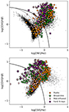 |
Fig. 2. Optical diagnostic diagrams for MaNGA galaxies. The black circles in the scatterplot show the emission-line ratio values for all MaNGA galaxies. In colored shapes, we feature the different AGN-selected candidates (see the legend). We took the flux ratio values from the ones measured around their central 2 kpc region (Albán & Wylezalek 2023). In the top panel, the gray line corresponds to the demarcation line from Kauffmann et al. (2003), and the black line (both in the top and bottom plots) corresponds to the ones from Kewley et al. (2001). |
We note that the hard X-ray-selected AGN candidates are the smallest sample. This is not surprising, as the BAT’s integration time is kept short to fulfill its scientific goals (Barthelmy et al. 2005). It is also the sample with the largest overlap with the other AGN samples; all X-ray-selected AGNs are also selected as AGNs in at least one other selection technique reported in this paper. Indeed, X-ray emission appears to be universal in AGNs and the emission is not significantly contaminated by its host galaxy (see a detailed discussion in Padovani et al. 2017). Hence, the optical, infrared, broad-line, and radio selection techniques make up the four biggest AGN subsamples in our study, with the largest number of independently selected candidates. Additionally, we have defined a sample of non-AGN galaxies that will be used in the discussion section. Our non-AGN sample contains all MaNGA galaxies that were not selected as AGNs by any method used in this paper.
3. Analysis
Hereinafter, when referring to kinematics, we specifically refer to the ionized gas (traced by the [O III] 5007 emission line).
3.1. Fitting procedure
Spectra from regions with kinematics dominated by winds can display complex emission-line profiles (e.g., Liu et al. 2013). This is not taken into account by the DAP emission-line fitting routine. Therefore, we developed a fitting procedure to account for up to two Gaussian components for each emission line. Our fitting method is based on a least-squares Python program using the documentation from nonlinear least squares minimization (LMFIT, Newville et al. 2016) and it follows standard fitting procedure techniques (e.g., Liu et al. 2013; Wylezalek et al. 2020). In summary, for all spectra in each MaNGA galaxy, our procedure operates in the rest-frame stellar-subtracted region where the [O III] 5007 emission line is (see the details in Appendix B). From the maps of the best-fit parameters, we created a nonparametric emission-line width W80 map. The W80 parameter is the most essential value we extracted from our fitting procedure and is the most relevant for the discussion throughout this paper. Whenever we refer to it, we refer to the W80 value obtained from [O III] 5007.
To study the spatial distribution of this parameter, we constructed radial profiles for all galaxies from elliptical annuli in steps of 0.25 effective radius (Reff). To obtain the parameters for the elliptical apertures for each galaxy, we used the b/a axis ratio and position angle (PA) from PIPE3D’s value-added catalog from Sánchez et al. (2022), as well as the effective radius. These parameters were adopted from the NASA-Sloan Atlas catalog (Blanton et al. 2011). They use the Petrosian system (see Petrosian 1976; Blanton et al. 2001) applied to the SDSS r-band imaging of galaxies using elliptical apertures. Here, Reff is defined as the major axis containing 50% of the flux inside 2 Petrosian radii, and b/a, and PA were obtained from the elliptical aperture (see the details in Wake et al. 2017). To perform a weighted average on each annulus, we captured the fraction of each pixel enclosed by an annulus so that we avoided average properties over a set of discrete pixels and recovered a smooth distribution. Specifically, we followed the pixel-weighted average procedure used in Albán & Wylezalek (2023) but using ellipses.
In a sample of ∼160 000 normal SDSS (SF BPT selected) galaxies (z < 0.7, with 8 < log(M*/M⊙) < 11.5 and −3 < log(SFR/M⊙yr−1) < 2), Cicone et al. (2016) find that the gas velocity dispersion (σ) hardly exceeds 150 km s−1. The latter corresponds to a W80 of ∼380 km s−1 (W80 = 2.56σ). Furthermore, Gatto et al. (2024) conclude a lower cut, of ∼315 km s−1, when studying the W80 in a control sample of non-AGNs (matched to optically selected AGNs in stellar mass, morphology, inclination, and redshift). Therefore, W80 values greater than this threshold suggest the presence of nongravitational motion of gas, such as outflows.
3.2. Galaxies selected for the kinematic analysis based on signal-to-noise quality criteria
One crucial factor to consider is the impact of the S/N on measuring the line width W80. As S/N decreases, the W80 measurements tend to get underestimated (see Liu et al. 2013), especially if there is indeed a (faint) broad component present in the line profile (Zakamska & Greene 2014). To ensure the accuracy of our analysis and avoid incorrect W80 measurements, we excluded all spaxels with an A/N < 7 (amplitude over noise) before we performed the spectral line fitting. Given the tight relation between S/N and A/N seen in Belfiore et al. (2019), we refer to A/N as simply S/N. To ensure that each individual galaxy retains enough high S/N spaxels, we furthermore applied the following criteria:
-
More than 10 spaxels with S/N > 7.
-
There are at least two annuli (for the radial profile derivation) where the area covered by the spaxels with an S/N > 7 is at least 10% of each annulus’s total area.
The thresholds for the S/N and pixel fractions were chosen to minimize the number of excluded galaxies, while retaining a suitable quality for the analysis. These quality cuts introduce a bias (driven by the S/N) that rejects galaxies that are more likely to be low in terms of SF, and some high-mass galaxies, respectively (e.g., Brinchmann et al. 2004; Albán & Wylezalek 2023). Our final sample contains 5696 targets (see the left plot in Fig. 3). Table 1 and Table 2 show the crossmatches between the different AGN populations and how the subsample sizes decrease after applying the S/N and quality cuts. Radio-selected AGN candidates are significantly impacted by the quality criteria (see Fig. 1). In contrast, the other AGN samples remain relatively unaffected.
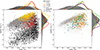 |
Fig. 3. Stellar mass versus star formation rates of MaNGA host galaxies. The left panel shows the impact of our quality criteria (see Sect. 3.2), excluding galaxies with higher stellar mass and lower star formation rates (represented by the black dots in the scatter plot and hatched black distribution in the top and right-hand diagrams). In red, orange, and yellow, we show the distribution of the AGN candidates selected by radio (using 0.0, 0.5, and 1.0 dex of excess; see Sect. 2.2.4) that satisfy the S/N quality criteria. To understand the properties of the excluded radio-selected hosts, we encourage the reader to look at Fig. 1. It can be seen that a long tail of deficient SFR hosts are excluded (−2> log(SFR(Hα)) > −4). On the right, we show only the galaxies chosen after the quality criteria and their corresponding AGN classifications. We have provided labels for each color in a panel between both plots. |
According to the optical classification from Albán & Wylezalek (2023), more than 90% of the radio-selected AGNs that were excluded from the final sample due to the quality criteria are LINERs (∼30%, with EW(Hα < 3)) or “lineless” (∼60%, galaxies that could not be classified by optical analysis, with S/N < 3; see the details in Albán & Wylezalek 2023), and around 5% are classified as ambiguous.
3.3. Typical properties of AGN-selected host galaxies
Focusing on the final sample of galaxies that fulfill the S/N and quality criteria, Fig. 4 shows host galaxy properties for our AGN populations, including a Venn4 diagram (following to Table 2). Comparing Table 1 with Table 2 (samples before and after the quality cuts) reveals that the AGN samples do not experience a significant cut, with the exception of radio-selected AGNs, where a notable fraction of massive galaxies with low SFR and low EW(Hα) got excluded (see Section 3.2). However, the distribution of b/a and L[O III] for radio-selected AGNs remains less affected by the S/N cut.
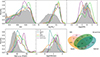 |
Fig. 4. Smooth histograms of multiple host galaxy properties. Top (left to right): b/a axis ratio, log(M⋆), and log(SFR) from Pipe3D. Bottom (left and middle plot): log(L[O III]) and log(EW(Hα)), both extracted from an aperture of 1 Reff, and (to the right) a complementary illustration for Table 2 employing Venn diagrams. In order to maintain visual clarity, the hard X-ray-selected AGN sample was intentionally omitted from the diagrams. The gray-shaded histogram shows the distribution of all MaNGA that pass our S/N criteria (see Sect. 3.2). |
Most AGNs are found in host galaxies with high stellar masses (M⋆; see the top-middle plot of Fig. 4), regardless of the AGN selection technique. This is a ubiquitous trend that has been found in various AGN samples from different studies (see e.g. Kauffmann et al. 2003; Powell et al. 2018; Barrows et al. 2021; Best et al. 2005). Our different AGN subsamples all have similar stellar mass distributions. This is an important fact to notice, given that more massive galaxies are expected to have larger emission-line widths (e.g., Chae 2011; Zahid et al. 2016; Cappellari 2016, see also Appendix C).
Figure 4 reveals that the different AGN samples probe different distributions of their host SFR, L[O III], and EW(Hα), showcasing the biases of each selection technique. The SFR differences between the samples are reflected in Fig. 3, where our AGN candidates tend to gather below the star formation main sequence (SFMS). The AGN studies for samples in the local Universe have found similar results, where AGNs are found in the so-called transition zone or the green valley (e.g., Schawinski et al. 2007; Salim 2014; Leslie et al. 2016). At slightly higher redshifts (0.25 < z < 0.8), Hickox et al. (2009) find that mid-infrared selected AGNs have bluer colors and are found preferentially in the blue cloud, while radio-selected AGNs are more likely to gather in the red sequence, suggesting that the latter are relevant for understanding the evolutionary transition of host galaxies from actively SF states to more quiescent ones.
Wylezalek et al. (2018) find that AGN-selected MaNGA (DR14) targets have mostly low to intermediate luminosities (L[O III] ∼ 1040 erg s−1) for an optically selected AGN sample. We observe here the same behavior for our optically selected AGNs in MaNGA-DR17. However, for AGNs selected via infrared, hard X-rays, or broad Balmer lines, we typically observe higher L[O III], with distributions peaking at ∼L[O III] ∼ 1041.6 erg s−1. On the other hand, radio-selected AGN candidates show some lower L[O III] values. Interestingly, L[O III] is known to correlate with the AGN’s bolometric luminosity (Heckman et al. 2004; LaMassa et al. 2010; Pennell et al. 2017), which in turn is correlated with AGN-driven wind velocities (e.g., Fiore et al. 2017).
Of the 288 radio-selected AGNs used in this analysis, 52 were optically classified as LINERs with AGNs (see Sect. 2.2.1) and 55 were not classified as AGNs as they did not meet the minimum Hα equivalent width of 3 Å. The 52 LINER galaxies have a median EW(Hα) of ∼1.75 Å. Other authors have used less strict EW(Hα) constraints (Sánchez et al. 2018, e.g., 1.5 Å) to include fainter AGNs in optically selected samples. However, this might introduce some LINER-like galaxies that have no AGN but that are dominated by a population of post-AGB stars (Singh et al. 2013) that can mimic AGN-like ionization in a typical optical classification. This emphasizes the importance of a multiwavelength AGN selection technique for a more complete population census. Quite remarkably, AGNs that were selected by mid-infrared, broad-lines, or X-ray observations clearly show EW(Hα) > 3.0 Å (only three galaxies have EW(Hα) < 3.0 Å ∼ 2.0 Å), while radio-selected AGNs show lower EW(Hα)∼2.0 Å. We recall that optically selected AGNs were required to have EW(Hα) > 3.0 Å (Albán & Wylezalek 2023). Therefore, we investigated whether the differences in the W80 radial profiles (see Sect. 3.4) can be attributed to any differences in host-galaxy properties.
3.4. Radial profiles of ionized gas kinematics
Several studies have investigated the overall AGN kinematic properties across many different AGN samples (e.g., Mullaney et al. 2013; Zakamska & Greene 2014; Baron & Netzer 2019; Rojas et al. 2019, among others). However, most of these studies have used single-fiber data and have therefore been limited in assessing spatial dependencies. Consequently, comprehensive studies with large spatially resolved spectral samples are crucial to assessing the impact of selection techniques. We investigated the radial profiles of ionized gas kinematics in the various AGN samples we have defined above. To do so, we first stacked the W80 profiles (see Sect. 3.1) of galaxies within each individual subsample and used the median value at each annulus.
The resulting profiles are shown in Fig. 5. The shaded regions around the profiles represent the 14th and 86th percentiles of the W80 distribution at each specific annulus. The median W80 profiles reveal distinct behaviors between the AGN samples. Visual inspection indicates variations not only in the magnitude but also in the slopes of these profiles. Notably, regardless of the AGN selection technique, there is a systematic behavior of an enhanced W80 profile in the AGN population compared to the overall MaNGA sample. This characteristic continues out to 2 effective radii. Similarly, if we focus only on galaxies that were not selected as AGNs by any of our selection techniques (the non-AGNs; see Sect. 2.2.5), we find the same trend. Moreover, SF-classified galaxies exhibit less pronounced profiles, with minimal enhancements near the center. The subsequent section will explore potential explanations for these observations.
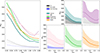 |
Fig. 5. W80 stacked radial profiles for various galaxy groups. In the upper central panel, the colors represent these groups: black, gray, and blue for all MaNGA galaxies, non-AGNs, and SF galaxies (selected by BPT), while the remaining colors denote AGN-selected candidates. Each line in the plots represents the median value at each Reff ring, with shaded areas indicating the 14th to 86th percentiles. The leftmost plot displays unshaded profiles for easier comparison. Different line styles are used for visual clarity. |
4. Results
Figure 5 (see the left panel) reveals that the median W80 radial profiles of AGN-selected populations are significantly different. In Sect. 3.3, we show that the host galaxies of the different AGN samples are similar with respect to some properties (e.g., stellar mass, or b/a axis ratio) but significantly different with respect to other properties (e.g., L[O III], or SFR(Hα)). We note that samples with higher M⋆ will systematically select galaxies with higher L[O III] and vice versa (see also Appendix C). At the same time, samples with higher M⋆ and L[O III] will systematically select galaxies with higher W80 (see the discussion in Sect. 3.3). Therefore, in this section, we investigate if and how the differences in the kinematics persist or change when we carefully match the AGN samples so that they have the same host galaxy properties.
We created control samples based on an M⋆ and L[O III] parameter space. Given that the number of galaxies per each M⋆ and L[O III] bin becomes limited, controlling for redshift and morphology becomes challenging. Therefore, we selected the galaxy that is closest in redshift and in morphology. The morphology was used as a number (obtained from Sánchez et al. 2022). We also note that the radial profiles take the Reff of each galaxy into account by using it as a step for the average W80 at each annulus (see Sect. 3.4).
4.1. AGNs versus non-AGNs
In a recent study, Gatto et al. (2024) used a catalog of optically selected AGNs (selected through emission-line diagnostics) and created a control sample matching properties to the AGN hosts similarly to in this paper, except for the L[O III]. When looking at all spaxels, they find that AGNs have greater W80 values than the control galaxies, attributing the ionized gas kinematic disturbances to the presence of the AGN. We obtain similar results to Gatto et al. (2024) (see Fig. 1) when using only optically selected AGNs and a similar control sample. In Fig. 6, we present the results as radial profiles for this comparison5, finding that optically selected AGNs have larger velocity widths than non-AGNs of similar masses. We find similar results when selecting AGNs through other techniques (see below).
 |
Fig. 6. Comparison of stacked W80 profiles and host galaxy properties between non-AGNs and optical AGNs. In each plot, blue corresponds to the behavior of a specific parameter for optically selected AGNs and black for non-AGNs. We show the W80 stacked radial profile, the log(M⋆) distribution, the log(L[O III]) distribution, and the log(SFR(Hα)) distribution. For this comparison, only log(M⋆), redshift, and morphology were controlled. |
Gatto et al. (2024) find that both AGNs and control galaxies have L[O III] values that correlate positively with their average W80. We see that their control sample has a median L[O III] that is ∼1 dex lower than the ones from an AGN. Therefore, in our analysis, we ask whether the kinematic differences are still present between non-AGNs and AGNs if L[O III] is taken into account during the control (this removes the most luminous AGNs). Under these conditions, we observe that AGNs and controls are more alike in terms of their W80 values (see the discussion in Sect. 5).
With this approach, we aim to assess the question of whether the current nuclear activity is responsible for the enhanced radial profiles in the AGN populations, and if so, to what extent these perturbations are spreading. We also seek to investigate how the kinematics may be dependent on the AGN selection technique. Therefore, we look at the W80 radial profiles comparing non-AGNs (see Figs. 7 and 8) with the following samples:
-
Sample A: Targets selected via optical or broad lines, excluding the ones selected via radio.
-
Sample B: Targets selected via radio but not via optical or broad lines.
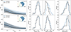 |
Fig. 7. Comparison of stacked W80 profiles and host galaxy properties between non-AGNs and sample A. In each plot, blue corresponds to the behavior of a specific parameter for sample A (see Sect. 4.1) and black for non-AGNs. For each column of plots, from left to right, we show the W80 stacked radial profile, the log(M⋆) distribution, the log(L[O III]) distribution, and the log(SFR(Hα)) distribution. The plots in the bottom row show how both samples behave after they are matched to have the same log(M⋆) and log(L[O III]). The plots in the top row show how both samples behave if the matching is done only for log(M⋆). The Venn diagrams shown in each W80 plot represent sample A. The discrepancy in the Venn diagram numbers in sample A arises from the incorporation of L[O III] into the control. |
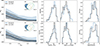 |
Fig. 8. Comparison of stacked W80 profiles and host galaxy properties between non-AGNs and sample B. Same as Fig. 7 but comparing non-AGNs (black) to sample B (blue). |
We do not observe a significant difference (in terms of ionized gas kinematics) between optically selected and broad-line-selected AGNs (see the details in Sect. 4.2). This is the main reason why we merged them when defining sample A and sample B for the purpose of comparing them with radio-selected AGNs.
We present a comparison between non-AGNs and AGNs, using as a control sample of non-AGNs first matched only in stellar mass, morphology, and redshift, and later including L[O III] in the parameter match (as was mentioned at the beginning of this section). Figure 7 shows two rows of plots. The top row shows the W80 radial profiles as well as histograms of host galaxy properties of sample A and non-AGNs without including L[O III] during the match. The bottom row shows the comparison considering L[O III] during the match. We note that the latter matching procedure leads to the removal of the most extreme AGNs in sample A exhibiting the highest L[O III]. The shaded areas in the radial profiles show the 14th and 86th percentiles as in Fig. 4, while the histograms report the M⋆ and L[O III] (both parameters used during the match) and the SFR(Hα) (same SFR used in Fig. 1), which was not used for the match.
The upper left plot shows that sample A has greater W80 values at all annuli than non-AGNs when only the M⋆ is considered during the match. We can see that L[O III] is systematically lower for non-AGNs. As was mentioned above, Gatto et al. (2024) find that their non-AGN control sample has [O III] line widths that correlate with [O III] luminosity. If we include the L[O III] (bottom left plot of Fig. 7), the median W80 value at all annuli of sample A and the non-AGN sample behaves similarly. While there might be a small difference at small radii Reff < 0.5, at large radii, there is no difference between both samples. This suggests that the stacked W80 radial profiles of optically selected AGNs together with broad-line-selected AGNs can be easily reproduced by non-AGN hosts with the same distribution of mass, M⋆, and L[O III].
In contrast to sample A, sample B (see Fig. 8) shows higher W80 values compared to non-AGNs. Remarkably, the most significant difference between non-AGNs and sample B is seen at the largest annuli, where high W80 values are achieved by sample B. Excluding optically (and broad-line) selected samples from our radio-selected AGNs systematically removes AGNs with low W80 at larger annuli. For sample A, it appears that excluding radio-selected AGNs from optically (or broad-line) selected samples consistently removes the W80 kinematic excess at larger annuli.
4.2. AGNs versus AGNs
In Fig. 4, we find that our broad-line-selected AGNs tend to have larger L[O III] than optically selected AGN galaxies. Therefore, in the top panel of Fig. 9, we match the two samples within 39.4 < log(L[O III]) < 42.1 and 10.4 < log(M⋆) < 11.7 (limits within which the parameter distribution can be matched) and compare the two samples: optically selected AGNs excluding broad-line-selected AGNs and vice versa. We find that the median W80 radial profile of broad-line-only AGNs is similar to the optically selected AGNs (excluding broad-line AGNs) when both samples are matched in host galaxy properties, with a small excess in the center for the broad-line-selected AGNs (see Fig. 9). Gatto et al. (2024) arrive at similar conclusions for their broad-line and optically selected AGNs, reporting no difference when comparing their W80 distributions. The results remain unchanged if we also control for inclination (b/a), ruling out possible orientation effects. Therefore, we combined these samples when setting up sample A and sample B (in Sect. 4.1).
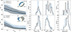 |
Fig. 9. Comparison of stacked W80 profiles and host galaxy properties between different AGN samples. The plots in the top and bottom rows show how both samples behave after they are matched to have the same log(M⋆) and log(L[O III]). The Venn diagrams shown in each W80 plot represent the AGN sample in the label. Top: Blue for optically selected (without broad-line-selected) and gray for the opposite. Bottom: Blue for sample B and gray for sample A. For each column of plots, from left to right, we show the W80 stacked radial profile, the log(M⋆) distribution, the log(L[O III]) distribution, and the log(SFR(Hα)) distribution. |
We now proceed with comparing sample A with sample B directly. As before, we also match the samples in M⋆ and L[O III], redshift and morphology. When excluding radio-selected sources from the optically selected AGN catalog (sample A), we do not claim that the remaining optically selected AGNs have no AGN-related radio emission, but we rather aim to investigate kinematic properties of a sample that would not have been detected as AGNs through radio techniques and vice versa.
In the bottom left panel of Fig. 9, we present the W80 radial profiles of sample A and sample B. Sample A is forced to match sample B within 39.2< log(L[O III]) < 41.5 and 10.1< log(M⋆) < 11.7. Sample B (represented in blue) shows elevated W80 values across all annuli, notably at large Reff, aligning with the findings in Sect. 4.1. This comparison suggests that while optical and broad-line selection methods can identify AGN hosts with perturbed kinematics extending to large galactocentric distances, the absence (or exclusion) of radio-selected AGNs (as in sample A, shown in gray) results in a population characterized by systematically reduced kinematic disturbances at these distances. Conversely, when optically and broad-line-selected AGNs are removed from a radio-selected sample (as in sample B), the remaining AGN hosts predominantly exhibit significant kinematic perturbations, especially at extended Reff scales. This suggests that AGN radio-selection techniques are sensitive to finding AGN hosts with disturbed kinematics over larger galactocentric distances.
A key takeaway message is that the selection technique is sensitive to the kinematics found in AGN galaxies and might also be sensitive to the evolutionary stage of the AGN (see the Discussion section). We point out that employing alternative cutoff lines in our radio selection technique (e.g., 1.5 dex; see Sect. 2.2.4 and Fig. 1) produces similar outcomes. As is illustrated in Fig. 4, a larger cutoff would also result in a cut in the stellar mass. However, this would also substantially reduce the number of targets. Our results concerning radio AGNs are very similar if we consider a different SFR estimator (as is mentioned in Sect. 2.2.4) when selecting our radio sample.
4.3. Star-forming galaxies versus AGNs
We performed a similar comparison between AGNs and (see Sect. 2.2.1) SF galaxies (as classified by BPT diagnostics). We find that SF galaxies have a lower median W80 radial profile compared to any of the AGN-selected samples (AGNs were excluded from the SF galaxy sample, although only 15 AGNs overlap with it). Furthermore, SF galaxies indeed have higher SFRs than our selected AGNs and even higher SFRs when controlling for M⋆ and L[O III] to a specific AGN selected population (they also have younger D4000 ages and higher Hα equivalent widths). This suggests that SF galaxies (at least, BPT-classified ones) in MaNGA do not seem to be responsible for driving significant ionized gas outflow signatures, even when they have significantly higher SFRs.
Lastly, in Sect. 3.2, we described how we only used galaxies with at least two available annuli where at least 10% of their spaxels have S/N > 7. This quality criteria results in some galaxies having no W80 values in some of their annuli. To control for a possible impact of this decision, we have studied the same comparisons described in this section with two samples: one where we use all the galaxies and all their spaxels that have a S/N > 3 (low S/N), and the other one where we only use galaxies that have at least six available annuli where at least 10% of their spaxels have S/N > 7 (a high S/N constraint). Using the latter samples, we confirm that the behavior described in this section is still present for all the comparisons.
5. Discussion
5.1. AGN selection and their integrated host galaxy properties
In this paper, we find that different AGN selection techniques select AGN samples that hardly overlap in more than 50% of their targets. Similar results have been found in Oh et al. (2022) at z < 0.2 when comparing X-ray-selected AGNs to optically selected ones. Additionally, for higher redshifts (0.25 < z < 0.8), in a sample of mid-infrared, radio, and X-ray-selected AGNs, Hickox et al. (2009) find that AGN candidates hardly overlap (their radio selection is at L1.4 GHz > 1023.8 W Hz−1). These findings pose a clear challenge for AGN studies, since AGNs found by the different selection techniques do not always trace the same host galaxy properties and/or AGN accretion state (Hickox & Alexander 2018).
We find that our radio-selected AGNs are typically found below the SFMS. Similar results have been found, specifically for MaNGA (Comerford et al. 2020; Mulcahey et al. 2022) and other low-redshift studies (e.g. Smolčić 2009). Accordingly, Sánchez et al. (2022) find that optically selected AGNs lie below the SFMS in the Green Valley. Additionally, Schawinski et al. (2007) find that SF galaxies, composite, and AGNs (all optically selected) seem to follow an evolutionary sequence in the star formation and stellar mass plane, with SF galaxies having bluer colors and AGNs found more in the transition zone. Our composite-selected targets are also found between SF and AGN-selected galaxies in the M⋆ versus SFR plane. Hickox et al. (2009) obtained similar results and were also in agreement with our mid-infrared selected targets, which they concluded are more likely to be found in slightly more SF hosts. They propose an evolutionary interpretation whereby, as star formation decreases, AGN accretion changes from optical or infrared-bright to optically faint radio sources. These findings suggest that AGN selection techniques are sensitive not only to the physical processes powering them but also to the stage of their duty cycle. We discuss this further in Sect. 5.3.
5.2. Spatially resolved ionized gas kinematics
We first investigated the radial properties of the [O III] ionized gas kinematics of unmatched AGNs and non-AGN samples, showcasing a diverse range of ionized gas kinematics (this was done before controlling for host galaxy properties; see Fig. 5). Non-AGN and SF galaxies exhibit less disturbed kinematics compared to all AGN samples (lower W80 radial profiles).
When comparing AGN samples matched in M⋆ and L[O III], intrinsic distinct kinematic behaviors emerge. Specifically, the exclusion of radio-selected AGNs from an optical and broad-line-selected AGN sample (sample A) results in lower W80 values at greater galactocentric distances, suggesting that much of the kinematic disturbances within an optically selected sample are linked to the radio emission in AGNs (see more discussion on the connection of outflows and radio emission in the next section).
The analysis of sample A also reveals that there is a population of non-AGN galaxies that can easily produce AGN-like W80 profiles when controlling for host galaxy properties (see bottom left panel of Fig. 7). Simulations suggest that kiloparsec-scale AGN-driven outflows can outlast the AGN activity phase, extending from a few to several orders of magnitude longer in duration (a few Myr, King et al. 2011; Zubovas 2018). For example, Zubovas et al. (2022) predict that fossil outflows (outflows taking place after the AGN switches off) could actually be more common than finding an outflow and an AGN in a galaxy simultaneously. Consequently, MaNGA non-AGN galaxies may include some galaxies showing fossil outflows. The possible presence of fossil outflows in MaNGA galaxies will be discussed in a future paper.
5.3. Radio-selected AGNs as tracers of the final phases of AGN evolution
We find that AGNs identified through radio techniques alone (sample B) show notably stronger kinematics at larger Reff than any other AGN sample. The presence of AGN-related radio emission in AGNs may therefore seem to trace AGNs with more spatially extended outflows.
One explanation for this behavior may be that sources with AGN-related radio emission trace host galaxies that have been experiencing AGN activity (or activities; see below) for a longer time. However, kinematic perturbances up to kiloparsec scales would typically imply an active (AGN) phase longer than the duration of a typical AGN duty cycle. For example, King et al. (2011) used analytical models to study the outflow propagation during an AGN event. They showed that an outflow with an initial velocity of a couple of hundred km s−1 in an AGN episode lasting about ∼1 Myr can last up to ten times longer than the AGN itself, reaching several kiloparsecs.
Alternatively, radio-selected AGNs may be sensitive to AGNs that have gone through multiple cycles of AGN activity. Indeed, some galaxies show evidence of past and recurring AGN events (e.g., Schawinski et al. 2015; Shulevski et al. 2015; Rao et al. 2023). Recent studies have used low-frequency (MHz) radio spectra combined with high-frequency (GHz) spectra to trace back emissions from previous activities (e.g., Jurlin et al. 2020). A younger AGN phase is characterized by a peaked spectrum in the center, while a remnant from past events displays a more spread-diffuse emission. Therefore, if a combination of the latter is observed in one target, it can suggest the target is a strong candidate for a restarted AGN phase. In this context, Kukreti et al. (2023) find that around 6% of the targets in their sample (at 1023 W Hz−1 > L1.4 GHz > 1026 W Hz−1, 0.02 < z < 0.23) are peaked sources classified as compact in GHz frequencies but have extended emission at MHz frequencies, suggesting that they are restarted AGN candidates.
Also, the simulations from Zubovas & Maskeliūnas (2023) show that fossil outflows in gas-poor systems tend to last longer than in gas-rich hosts. Radio-selected AGNs, indeed, are preferentially found in gas-poor galaxies.
With respect to an AGN’s impact on its host galaxy, a recent review by Harrison & Ramos Almeida (2024) discusses that simulations predict that feedback that leads to galaxy quenching does not come from a single AGN event but is rather a cumulative effect of multiple AGN episodes (see also Piotrowska et al. 2022). Thus, given the findings in our analysis, AGNs selected through radio observations may preferentially trace galaxies that have experienced episodic AGN events (Morganti 2017a). Sample B indeed contains host galaxies with older stellar populations (compared to sample A), traced by average D4000 measurements from the PiPE3D catalog.
In a sample of radio-selected AGNs from MaNGA MPL-8, Comerford et al. (2020) find that radio-mode AGN-hosting galaxies reside preferentially in elliptical galaxies that have more negative stellar age gradients with galactocentric distance. The authors suggest that radio-mode AGNs may represent a final phase in the evolution of an AGN. In addition, Hickox et al. (2009) proposed a scenario in which radio AGNs are key to the late stages of galaxy evolution, with them being in general more passive and having lower Eddington ratios than their infrared and optical counterparts. In fact, radio-selected AGNs typically have larger black hole masses (Best et al. 2005; Hickox et al. 2009). Interestingly, the latter parameter is found to be a strong predictor for galaxy quenching (Piotrowska et al. 2022). These results are in line with the work presented here on the spatially resolved ionized gas kinematics in radio-selected AGNs, which suggests that radio selection methods may be used to identify AGNs at a more advanced stage of their activity (and feedback) cycle. Lastly, we note that most of the removed radio-selected AGNs (see Sects. 3.2 and 3.3) are massive galaxies with low SFRs (see Fig. 1), located near the red sequence, suggesting an even later evolutionary phase.
5.4. The connection between radio-emission and outflow activity in AGNs
Our results discussed above raise the question of what mechanisms are responsible for the observed radio emissions. The possible origins of radio emission in low-luminosity radio AGNs is reviewed in Panessa et al. (2019). The review discusses several mechanisms such as jets, winds, accretion disk corona, and star formation. In the context of our work, winds are discussed as a mechanism in which a shock is driven by the wind (e.g., Riffel et al. 2021) and produce radio emission due to the acceleration of relativistic electrons on sub-kiloparsec scales. Similarly, in a small sample of AGNs (z < 0.07), Mizumoto et al. (2024) found that NLR-scale shocks (traced by [Fe II]/[P II]; see Oliva et al. 2001) are likely triggered by ionized outflows (traced by [S III] in Mizumoto et al. 2024).
Notably, in a sample of galaxies at z < 0.8, Zakamska & Greene (2014) show that the radio luminosity in formally radio-quiet AGNs correlates with the [O III] velocity width, which is consistent with our findings. Zakamska & Greene (2014) propose two scenarios: one in which radio emission is produced by accelerated particles as a result of shock fronts due to outflows (extended and diffuse radio emission), and another one in which an unresolved radio jet (unresolved in FIRST/NVSS data) is launching an outflow (expected to be compact). We argue that both scenarios could simultaneously be present in one system (e.g., if the galaxy had more than one recent AGN event). High-spatial-resolution radio observations would be needed to distinguish between them.
Calistro Rivera et al. (2024) arrive at similar conclusions by analyzing the CIV and [O III] velocities (in a sample of ∼100 AGNs). They discover minimal or no correlation between the CIV velocities and radio luminosity, in contrast to a connection between the [O III] velocity width and radio luminosity. Given that CIV emission originate from within the broad-line region (sub-parsec scales), and [O III] emission traces ionized gas on galactic or kiloparsec scales, Calistro Rivera et al. (2024) conclude that the interplay between winds and radio luminosity predominantly occurs on these circumnuclear scales. Similarly, Liao et al. (2024) not only shows that [O III] velocity widths of AGNs (in their sample: z < 1.0, and a median log(L[O III])∼42.1) correlate with radio emission but also that the conversion efficiencies align with those needed to account for the observed radio luminosities in galaxies exhibiting large [O III] velocity widths. Their results also support the idea that AGN-driven outflows contribute to the radio emission in AGNs.
While the results discussed above suggest a connection between the radio emission and the ionized gas kinematics in AGNs, we note that they were done predominantly using single fiber spectra and investigating higher-redshift galaxies (z ≲ 0.8), averaging the gas kinematics over larger areas. Our work adds to the picture using a spatially resolved kinematic analysis and while we cannot exclude the presence of jetted radio-AGNs in our radio-selected sample, our results also suggest that there is a strong connection between radio activity and ionized gas outflows in AGNs.
5.5. Star-forming galaxies
We find that SF galaxies show less enhanced kinematic profiles when compared to AGN candidates, even when controlling for M⋆, L[O III], morphology, and redshift. A detailed comparison between sample A and SF galaxies highlights that sample A demonstrates significantly higher W80 values within its central regions. In contrast, such differences fade at larger effective radii (Reff), where the kinematic behaviors of both populations (sample A and the matched star formation sample) align closely. Moreover, the matched SF galaxy sample exhibits higher star formation rates than sample A (and higher than the SF sample before matching). In a larger sample (> 50 000) of local (0.05 < z < 0.1) SF galaxies, Yu et al. (2022) study the ionized gas kinematics of these galaxies, finding that they can indeed present outflow signatures. But the authors also show that the SF sample hardly ever reaches σ > 150 km s−1; that is, W80 > 375 km s−1. This is consistent with our findings. Therefore, we infer that the enhanced W80 values in our AGN-selected population are likely driven by AGNs and do not expect SF processes to play a significant role.
However, the most massive (M⋆ > 1011 M⊙) SF galaxies in our sample reveal remarkably high W80 values (although not as high as those of AGNs). Sabater et al. (2019) found that 100% of the galaxies with masses above this limit (1011 M⊙) host radio AGNs even though sometimes with radio luminosities (L150 MHz > 1021.5 W Hz−1, or L1.4 GHz ≳ 1021 W Hz−1; most of our galaxies are above this limit). Indeed, > 50% of massive SF galaxies in our sample have radio detections, while only ∼10% of lower-mass SF galaxies (< 1011 M⊙) have radio detections. This suggests that some of our massive SF galaxy populations may be AGNs as well.
6. Summary and conclusions
We have assembled a multiwavelength AGN-selected sample for the SDSS-IV MaNGA-DR17, comprising 594 unique AGNs identified through optical, hard X-ray, radio, infrared, and broad-line selection techniques. We seek to explore the extent to which ionized gas kinematics, quantified by W80 of [O III]λ5007, is influenced by the diversity in AGN selection methods, thereby offering insights into feedback processes and the duty cycle of AGN activity. To do so, we fit up to two Gaussian components to the [O III]λ5007 emission-line region in all spaxels (S/N > 7; see Sect. 3.2) of each galaxy and derived the W80 velocity widths (see Sect. 4). We then mapped the spatial distribution of this parameter for each galaxy. Furthermore, we created W80 radial profiles and stacked them according to each defined AGN subsample. Our findings are summarized as follows:
-
We find that different AGN selection techniques do not completely overlap with each other. Overlap ranges from ∼34% (e.g., between radio and optical selection) up to ∼80% (the latter percentage only achieved by the X-ray selection, although it is the smallest sample).
-
The different AGN populations are found in galaxies with different host galaxy properties. The most significant differences are found in the distribution of L[O III], EW(Hα), D4000, and the W80 radial profiles.
-
Regarding AGNs versus non-AGNs: Regardless of the selection technique, all AGN populations show more perturbed ionized gas kinematics (traced by W80) at all annuli when compared to non-AGNs of similar M⋆ of the host, redshift, and morphology. These kinematic differences become less pronounced when L[O III] is taken into account in the non-AGN control sample. Remarkably, the differences between AGNs and non-AGNs disappear when we compare pure optical (BPT and broad-line, but excluding radio-detect AGNs: sample A) AGNs to non-AGNs (see Sect. 4.1). We suggest that some non-AGNs may host fossil outflows (i.e., relic outflows of a past AGN phase), which may outnumber outflows in currently active AGNs (Zubovas et al. 2022).
-
Regarding AGNs versus AGNs: Our different AGN samples display not only hosts with different properties but also hosts with differences in the stacked radial profiles of their kinematic signatures. Interestingly, when controlling for host galaxy properties, we find that removing radio-selected AGNs from optically selected candidates leaves a sample (sample A) of galaxies that lack significantly high W80 at high Reff, suggesting that many of the kinematic disturbances within an optically selected sample are linked to the radio emission in AGNs. In addition, radio-selected AGNs show more enhanced ionized gas kinematics at all radii and their hosts show evidence of older stellar populations. Our results support a scenario in which radio selection methods may be used to identify AGNs at a more advanced stage of their activity (and feedback) cycle.
-
AGNs versus SF galaxies: SF galaxies in our sample do not show significant kinematic signatures in the ionized gas compared to AGNs (regardless of the selection technique; see Sect. 2). We highlight that when controlling for L[O III] and M⋆ when comparing AGNs to non-AGNs, SF galaxies tend to have significantly larger SFR(Hα) than AGNs. We conclude that in our sample the main driver of the enhanced kinematic signatures in AGNs cannot be accounted for by star formation processes alone.
Our study shows that a given AGN selection technique can impact what sorts of ionized kinematic signatures are found in their host galaxies. Our results have been tested in low-redshift (z < 0.1) galaxies with low to intermediate luminosities. The impact of AGN selection techniques could be more significant at higher redshift. Moreover, our results highlight the importance and utility of spatially resolved spectroscopy.
The equivalent width of each galaxy was obtained using the same aperture size used to measure the emission-line ratios during the classification. Equivalent widths and emission-line ratios are also included in the Albán & Wylezalek (2023) catalog.
Note that the catalog from Albán & Wylezalek (2023) originally reports 419 targets using a 2 kpc aperture. However, we excluded galaxies due to duplication or critical flags (see Appendix A).
We create our Venn diagrams from an adapted version of this public repository: https://github.com/tctianchi/pyvenn
We used our non-AGN sample, i.e., also removing AGNs selected by a multiwavelength selection, as is discussed in Sect. 2.2.
Acknowledgments
D.W. acknowledges support through an Emmy Noether Grant of the German Research Foundation, a stipend by the Daimler and Benz Foundation and a Verbundforschung grant by the German Space Agency. M.A. extends gratitude to the GALENA research group for their invaluable discussions, which have significantly shaped the ideas presented in this paper. M.A. also wishes to acknowledge Chris Harrison for his engaging conversations at conferences, which played a key role in developing the early stages of this paper. J.M.C. is supported by NSF AST-1714503 and NSF AST- 1847938. RAR acknowledges the support from Conselho Nacional de Desenvolvimento Científico e Tecnológico (CNPq; Proj. 303450/2022-3, 403398/2023-1, & 441722/2023-7), Fundação de Amparo à pesquisa do Estado do Rio Grande do Sul (FAPERGS; Proj. 21/2551-0002018-0), and CAPES (Proj. 88887.894973/2023-00). This project makes use of the MaNGA-Pipe3D dataproducts. We thank the IA-UNAM MaNGA team for creating this catalogue, and the Conacyt Project CB-285080 for supporting them. Funding for the Sloan Digital Sky Survey IV has been provided by the Alfred P. Sloan Foundation, the U.S. Department of Energy Office of Science, and the Participating Institutions. SDSS-IV acknowledges support and resources from the Center for HighPerformance Computing at the University of Utah. The SDSS web site is http://www.sdss.org. SDSS-IV is managed by the Astrophysical Research Consortium for the Participating Institutions of the SDSS Collaboration including the Brazilian Participation Group, the Carnegie Institution for Science, Carnegie Mellon University, the Chilean Participation Group, the French Participation Group, Harvard-Smithsonian Center for Astrophysics, Instituto de Astrofísica de Canarias, The Johns Hopkins University, Kavli Institute for the Physics and Mathematics of the Universe (IPMU) / University of Tokyo, the Korean Participation Group, Lawrence Berkeley National Laboratory, Leibniz Institut für Astrophysik Potsdam (AIP), Max-Planck-Institut für Astronomie (MPIA Heidelberg), Max-Planck-Institut für Astrophysik (MPA Garching), Max-Planck-Institut für Extraterrestrische Physik (MPE), National Astronomical Observatories of China, New Mexico State University, New York University, University of Notre Dame, Observatario Nacional/MCTI, The Ohio State University, Pennsylvania State University, Shanghai Astronomical Observatory, United Kingdom Participation Group, Universidad Nacional Autonoma de México, University of Arizona, University of Colorado Boulder, University of Oxford, University of Portsmouth, University of Utah, University of Virginia, University
References
- Aalto, S., Garcia-Burillo, S., Muller, S., et al. 2012, A&A, 537, A44 [NASA ADS] [CrossRef] [EDP Sciences] [Google Scholar]
- Aird, J., Coil, A. L., Georgakakis, A., et al. 2015, MNRAS, 451, 1892 [Google Scholar]
- Albán, M., & Wylezalek, D. 2023, A&A, 674, A85 [NASA ADS] [CrossRef] [EDP Sciences] [Google Scholar]
- Alberts, S., Rujopakarn, W., Rieke, G. H., Jagannathan, P., & Nyland, K. 2020, ApJ, 901, 168 [NASA ADS] [CrossRef] [Google Scholar]
- Alexander, D. M., & Hickox, R. C. 2012, New Astron. Rev., 56, 93 [Google Scholar]
- Andrae, R., Schulze-Hartung, T., & Melchior, P. 2010, Dos and don’ts of reduced chi-squared [Google Scholar]
- Baldwin, J. A., Phillips, M. M., & Terlevich, R. 1981, PASP, 93, 5 [Google Scholar]
- Baron, D., & Netzer, H. 2019, MNRAS, 482, 3915 [Google Scholar]
- Baron, D., Netzer, H., Lutz, D., Prochaska, J. X., & Davies, R. I. 2021, MNRAS, 509, 4457 [NASA ADS] [CrossRef] [Google Scholar]
- Barrows, R. S., Comerford, J. M., Stern, D., & Assef, R. J. 2021, ApJ, 922, 179 [NASA ADS] [CrossRef] [Google Scholar]
- Barthelmy, S. D., Barbier, L. M., Cummings, J. R., et al. 2005, Space Sci. Rev., 120, 143 [Google Scholar]
- Becker, R. H., White, R. L., & Helfand, D. J. 1995, ApJ, 450, 559 [Google Scholar]
- Belfiore, F., Westfall, K. B., Schaefer, A., et al. 2019, AJ, 158, 160 [CrossRef] [Google Scholar]
- Bennert, N., Jungwiert, B., Komossa, S., Haas, M., & Chini, R. 2006, A&A, 456, 953 [NASA ADS] [CrossRef] [EDP Sciences] [Google Scholar]
- Best, P. N., & Heckman, T. M. 2012, MNRAS, 421, 1569 [NASA ADS] [CrossRef] [Google Scholar]
- Best, P. N., Kauffmann, G., Heckman, T. M., & Ivezić, Ž. 2005, MNRAS, 362, 9 [Google Scholar]
- Blanton, M. R., Dalcanton, J., Eisenstein, D., et al. 2001, AJ, 121, 2358 [NASA ADS] [CrossRef] [Google Scholar]
- Blanton, M. R., Kazin, E., Muna, D., Weaver, B. A., & Price-Whelan, A. 2011, AJ, 142, 31 [NASA ADS] [CrossRef] [Google Scholar]
- Brinchmann, J., Charlot, S., White, S. D. M., et al. 2004, MNRAS, 351, 1151 [Google Scholar]
- Bundy, K., Bershady, M. A., Law, D. R., et al. 2015, ApJ, 798, 7 [Google Scholar]
- Calistro Rivera, G., Alexander, D. M., Harrison, C. M., et al. 2024, A&A in press, https://doi.org/10.1051/0004-6361/202348982 [Google Scholar]
- Cappellari, M. 2016, ARA&A, 54, 597 [Google Scholar]
- Chae, K.-H. 2011, MNRAS, 413, 887 [NASA ADS] [CrossRef] [Google Scholar]
- Cheung, E., Bundy, K., Cappellari, M., et al. 2016, Nature, 533, 504 [NASA ADS] [CrossRef] [Google Scholar]
- Cicone, C., Maiolino, R., Sturm, E., et al. 2014, A&A, 562, A21 [NASA ADS] [CrossRef] [EDP Sciences] [Google Scholar]
- Cicone, C., Maiolino, R., & Marconi, A. 2016, A&A, 588, A41 [NASA ADS] [CrossRef] [EDP Sciences] [Google Scholar]
- Cid Fernandes, R., Stasinska, G., Schlickmann, M. S., et al. 2010, MNRAS, 403, 1036 [NASA ADS] [CrossRef] [Google Scholar]
- Comerford, J. M., Negus, J., Müller-Sánchez, F., et al. 2020, ApJ, 901, 159 [NASA ADS] [CrossRef] [Google Scholar]
- Comerford, J. M., Nevin, R., Negus, J., et al. 2024, ApJ, 963, 53 [NASA ADS] [CrossRef] [Google Scholar]
- Condon, J. J., Cotton, W. D., Greisen, E. W., et al. 1998, AJ, 115, 1693 [Google Scholar]
- DiPompeo, M. A., Hickox, R. C., Carroll, C. M., et al. 2018, ApJ, 856, 76 [Google Scholar]
- Fabian, A. 2012, ARA&A, 50, 455 [CrossRef] [Google Scholar]
- Ferrarese, L., & Merritt, D. 2000, ApJ, 539, L9 [Google Scholar]
- Fiore, F., Feruglio, C., Shankar, F., et al. 2017, A&A, 601, A143 [NASA ADS] [CrossRef] [EDP Sciences] [Google Scholar]
- Förster Schreiber, N. M., Genzel, R., Newman, S. F., et al. 2014, ApJ, 787, 38 [Google Scholar]
- Fu, Y., Cappellari, M., Mao, S., et al. 2023, MNRAS, 524, 5827 [CrossRef] [Google Scholar]
- Gatto, L., Storchi-Bergmann, T., Riffel, R. A., et al. 2024, MNRAS, 530, 3059 [NASA ADS] [CrossRef] [Google Scholar]
- Halpern, J. P., & Steiner, J. E. 1983, ApJ, 269, L37 [CrossRef] [Google Scholar]
- Harrison, C. M. 2017, Nat. Astron., 1, 0165 [NASA ADS] [CrossRef] [Google Scholar]
- Harrison, C. M., & Ramos Almeida, C. 2024, Galaxies, 12, 17 [NASA ADS] [CrossRef] [Google Scholar]
- Harrison, C. M., Alexander, D. M., Mullaney, J. R., & Swinbank, A. M. 2014, MNRAS, 441, 3306 [Google Scholar]
- Heckman, T. M., & Best, P. N. 2014, ARA&A, 52, 589 [Google Scholar]
- Heckman, T. M., Miley, G. K., van Breugel, W. J. M., & Butcher, H. R. 1981, ApJ, 247, 403 [NASA ADS] [CrossRef] [Google Scholar]
- Heckman, T. M., Kauffmann, G., Brinchmann, J., et al. 2004, ApJ, 613, 109 [Google Scholar]
- Herrera-Camus, R., Janssen, A., Sturm, E., et al. 2020, A&A, 635, A47 [NASA ADS] [CrossRef] [EDP Sciences] [Google Scholar]
- Hickox, R. C., & Alexander, D. M. 2018, ARA&A, 56, 625 [Google Scholar]
- Hickox, R. C., Jones, C., Forman, W. R., et al. 2009, ApJ, 696, 891 [Google Scholar]
- Hopkins, P. F., Hernquist, L., Cox, T. J., et al. 2006, ApJS, 163, 1 [Google Scholar]
- Ivezić, Ž., Menou, K., Knapp, G. R., et al. 2002, AJ, 124, 2364 [CrossRef] [Google Scholar]
- Jarvis, M. E., Harrison, C. M., Thomson, A. P., et al. 2019, MNRAS, 485, 2710 [Google Scholar]
- Jarvis, M. E., Harrison, C. M., Mainieri, V., et al. 2021, MNRAS, 503, 1780 [NASA ADS] [CrossRef] [Google Scholar]
- Ji, Z., Giavalisco, M., Kirkpatrick, A., et al. 2022, ApJ, 925, 74 [NASA ADS] [CrossRef] [Google Scholar]
- Jurlin, N., Morganti, R., Brienza, M., et al. 2020, A&A, 638, A34 [EDP Sciences] [Google Scholar]
- Karouzos, M., Woo, J.-H., & Bae, H.-J. 2016, ApJ, 819, 148 [NASA ADS] [CrossRef] [Google Scholar]
- Kauffmann, G. 2018, MNRAS, 480, 3201 [NASA ADS] [CrossRef] [Google Scholar]
- Kauffmann, G., Heckman, T. M., Tremonti, C., et al. 2003, MNRAS, 346, 1055 [Google Scholar]
- Kauffmann, G., Heckman, T. M., & Best, P. N. 2008, MNRAS, 384, 953 [Google Scholar]
- Kewley, L. J., Dopita, M. A., Sutherland, R. S., Heisler, C. A., & Trevena, J. 2001, ApJ, 556, 121 [Google Scholar]
- King, A., & Pounds, K. 2015, ARA&A, 53, 115 [NASA ADS] [CrossRef] [Google Scholar]
- King, A. R., Zubovas, K., & Power, C. 2011, MNRAS, 415, L6 [NASA ADS] [CrossRef] [Google Scholar]
- Kormendy, J., & Ho, L. C. 2013, ARA&A, 51, 511 [Google Scholar]
- Kukreti, P., Morganti, R., Tadhunter, C., & Santoro, F. 2023, A&A, 674, A198 [NASA ADS] [CrossRef] [EDP Sciences] [Google Scholar]
- Lacerda, E. A. D., Sánchez, S. F., Mejía-Narváez, A., et al. 2022, New Astron., 97, 101895 [NASA ADS] [CrossRef] [Google Scholar]
- Laker, M. A., Camacho, C. D., Jones, D., & Moody, J. 2022, Symmetry, 14, 2 [Google Scholar]
- LaMassa, S. M., Heckman, T. M., Ptak, A., et al. 2010, ApJ, 720, 786 [NASA ADS] [CrossRef] [Google Scholar]
- Law, D. R., Yan, R., Bershady, M. A., et al. 2015, AJ, 150, 19 [CrossRef] [Google Scholar]
- Leslie, S. K., Kewley, L. J., Sanders, D. B., & Lee, N. 2016, MNRAS, 455, L82 [NASA ADS] [CrossRef] [Google Scholar]
- Liao, M., Wang, J., Ren, W., & Zhou, M. 2024, MNRAS, 528, 3696 [NASA ADS] [CrossRef] [Google Scholar]
- Liu, X., Greene, J. E., Shen, Y., & Strauss, M. A. 2010, ApJ, 715, L30 [NASA ADS] [CrossRef] [Google Scholar]
- Liu, G., Zakamska, N. L., Greene, J. E., Nesvadba, N. P. H., & Liu, X. 2013, MNRAS, 436, 2576 [NASA ADS] [CrossRef] [Google Scholar]
- Luo, R., Woo, J.-H., Karouzos, M., et al. 2021, ApJ, 908, 221 [NASA ADS] [CrossRef] [Google Scholar]
- Madau, P., & Dickinson, M. 2014, ARA&A, 52, 415 [Google Scholar]
- Marconi, A., & Hunt, L. K. 2003, ApJ, 589, L21 [Google Scholar]
- Mizumoto, M., Sameshima, H., Kobayashi, N., et al. 2024, ApJ, 960, 41 [NASA ADS] [CrossRef] [Google Scholar]
- Molyneux, S. J., Harrison, C. M., & Jarvis, M. E. 2019, A&A, 631, A132 [NASA ADS] [CrossRef] [EDP Sciences] [Google Scholar]
- Morganti, R. 2017a, Nat. Astron., 1, 596 [Google Scholar]
- Morganti, R. 2017b, Front. Astron. Space Sci., 4, 42 [CrossRef] [Google Scholar]
- Mulcahey, C. R., Leslie, S. K., Jackson, T. M., et al. 2022, A&A, 665, A144 [NASA ADS] [CrossRef] [EDP Sciences] [Google Scholar]
- Mullaney, J. R., Alexander, D. M., Fine, S., et al. 2013, MNRAS, 433, 622 [Google Scholar]
- Naab, T., & Ostriker, J. P. 2017, ARA&A, 55, 59 [Google Scholar]
- Netzer, H. 2006, in Active Galactic Nuclei: Basic Physics and Main Components, eds. D. Alloin, R. Johnson,, & P. Lira (Berlin, Heidelberg: Springer) [Google Scholar]
- Netzer, H. 2015, ARA&A, 53, 365 [Google Scholar]
- Newville, M., Stensitzki, T., Allen, D. B., et al. 2016, Lmfit: Non-Linear Least-Square Minimization and Curve-Fitting for Python, Astrophysics Source Code Library [record ascl:1606.014] [Google Scholar]
- Oh, K., Yi, S. K., Schawinski, K., et al. 2015, ApJS, 219, 1 [Google Scholar]
- Oh, K., Koss, M. J., Ueda, Y., et al. 2022, ApJS, 261, 4 [NASA ADS] [CrossRef] [Google Scholar]
- Oliva, E., Marconi, A., Maiolino, R., et al. 2001, A&A, 369, L5 [NASA ADS] [CrossRef] [EDP Sciences] [Google Scholar]
- Osterbrock, D. 1989, Astrophysics of Gaseous Nebulae and ActiveGalactic Nuclei, A Series of Books in Astronomy (University Science Books) [Google Scholar]
- Padovani, P. 2016, A&ARv, 24, 13 [Google Scholar]
- Padovani, P. 2017, Front. Astron. Space Sci., 4, 35 [CrossRef] [Google Scholar]
- Padovani, P., Alexander, D. M., Assef, R. J., et al. 2017, A&ARv, 25, 2 [Google Scholar]
- Pan, H.-A., Lin, L., Hsieh, B.-C., et al. 2019, ApJ, 881, 119 [NASA ADS] [Google Scholar]
- Panessa, F., Baldi, R. D., Laor, A., et al. 2019, Nat. Astron., 3, 387 [Google Scholar]
- Pennell, A., Runnoe, J. C., & Brotherton, M. S. 2017, MNRAS, 468, 1433 [NASA ADS] [CrossRef] [Google Scholar]
- Peterson, B. M. 2006, in Physics of Active Galactic Nuclei at all Scales, ed. D. Alloin, 693, 77 [NASA ADS] [CrossRef] [Google Scholar]
- Petrosian, V. 1976, ApJ, 210, L53 [NASA ADS] [CrossRef] [Google Scholar]
- Piotrowska, J. M., Bluck, A. F. L., Maiolino, R., & Peng, Y. 2022, MNRAS, 512, 1052 [NASA ADS] [CrossRef] [Google Scholar]
- Powell, M. C., Cappelluti, N., Urry, C. M., et al. 2018, ApJ, 858, 110 [Google Scholar]
- Rao, V. V., Kharb, P., Rubinur, K., et al. 2023, MNRAS, 524, 1615 [NASA ADS] [CrossRef] [Google Scholar]
- Ricci, C., & Trakhtenbrot, B. 2023, Nat. Astron., 7, 1282 [Google Scholar]
- Riffel, R. A., Bianchin, M., Riffel, R., et al. 2021, MNRAS, 503, 5161 [NASA ADS] [CrossRef] [Google Scholar]
- Riffel, R. A., Storchi-Bergmann, T., Riffel, R., et al. 2023, MNRAS, 521, 1832 [NASA ADS] [CrossRef] [Google Scholar]
- Rojas, A. F., Sani, E., Gavignaud, I., et al. 2019, MNRAS, 491, 5867 [Google Scholar]
- Sabater, J., Best, P. N., Hardcastle, M. J., et al. 2019, A&A, 622, A17 [NASA ADS] [CrossRef] [EDP Sciences] [Google Scholar]
- Salim, S. 2014, SAJ, 189, 1 [Google Scholar]
- Sánchez, S. F., Avila-Reese, V., Hernandez-Toledo, H., et al. 2018, Rev. Mex. Astron. Astrofis., 54, 217 [Google Scholar]
- Sánchez, S. F., Barrera-Ballesteros, J. K., Lacerda, E., et al. 2022, ApJS, 262, 36 [CrossRef] [Google Scholar]
- Schawinski, K., Thomas, D., Sarzi, M., et al. 2007, MNRAS, 382, 1415 [Google Scholar]
- Schawinski, K., Koss, M., Berney, S., & Sartori, L. F. 2015, MNRAS, 451, 2517 [Google Scholar]
- Shulevski, A., Morganti, R., Barthel, P. D., et al. 2015, A&A, 583, A89 [NASA ADS] [CrossRef] [EDP Sciences] [Google Scholar]
- Silk, J., & Rees, M. J. 1998, A&A, 331, L1 [NASA ADS] [Google Scholar]
- Singh, R., van de Ven, G., Jahnke, K., et al. 2013, A&A, 558, A43 [NASA ADS] [CrossRef] [EDP Sciences] [Google Scholar]
- Singha, M., Husemann, B., Urrutia, T., et al. 2022, A&A, 659, A123 [NASA ADS] [CrossRef] [EDP Sciences] [Google Scholar]
- Smolčić, V. 2009, ApJ, 699, L43 [Google Scholar]
- Somerville, R. S., & Davé, R. 2015, ARA&A, 53, 51 [Google Scholar]
- Storey, P. J., & Zeippen, C. J. 2000, MNRAS, 312, 813 [NASA ADS] [CrossRef] [Google Scholar]
- Sun, A.-L., Greene, J. E., & Zakamska, N. L. 2017, ApJ, 835, 222 [Google Scholar]
- Suresh, A., & Blanton, M. R. 2024, ArXiv e-prints [arXiv:2404.04780] [Google Scholar]
- Tombesi, F., Cappi, M., Sambruna, R. M., et al. 2012, ASP Conf. Ser., 460, 8 [NASA ADS] [Google Scholar]
- Urry, C. M., & Padovani, P. 1995, PASP, 107, 803 [NASA ADS] [CrossRef] [Google Scholar]
- Veilleux, S., & Osterbrock, D. E. 1987, ApJS, 63, 295 [Google Scholar]
- Wake, D. A., Bundy, K., Diamond-Stanic, A. M., et al. 2017, AJ, 154, 86 [Google Scholar]
- Westfall, K. B., Cappellari, M., Bershady, M. A., et al. 2019, AJ, 158, 231 [Google Scholar]
- White, S. V., Jarvis, M. J., Häußler, B., & Maddox, N. 2015, MNRAS, 448, 2665 [Google Scholar]
- Woo, J.-H., Bae, H.-J., Son, D., & Karouzos, M. 2016, ApJ, 817, 108 [Google Scholar]
- Worrall, D., & Birkinshaw, M. 2006, in Multiwavelength Evidence of the Physical Processes in Radio Jets, eds. D. Alloin, R. Johnson, & P. Lira (Berlin, Heidelberg: Springer), 39 [Google Scholar]
- Wright, E. L., Eisenhardt, P. R. M., Mainzer, A. K., et al. 2010, AJ, 140, 1868 [Google Scholar]
- Wylezalek, D., Zakamska, N. L., Greene, J. E., et al. 2018, MNRAS, 474, 1499 [NASA ADS] [CrossRef] [Google Scholar]
- Wylezalek, D., Flores, A. M., Zakamska, N. L., Greene, J. E., & Riffel, R. A. 2020, MNRAS, 492, 4680 [NASA ADS] [CrossRef] [Google Scholar]
- Yu, B. P. B., Angthopo, J., Ferreras, I., & Wu, K. 2022, PASA, 39, e054 [NASA ADS] [CrossRef] [Google Scholar]
- Zahid, H. J., Geller, M. J., Fabricant, D. G., & Hwang, H. S. 2016, ApJ, 832, 203 [NASA ADS] [CrossRef] [Google Scholar]
- Zakamska, N. L., & Greene, J. E. 2014, MNRAS, 442, 784 [Google Scholar]
- Zakamska, N. L., Hamann, F., Pâris, I., et al. 2016a, MNRAS, 459, 3144 [NASA ADS] [CrossRef] [Google Scholar]
- Zakamska, N. L., Lampayan, K., Petric, A., et al. 2016b, MNRAS, 455, 4191 [Google Scholar]
- Zubovas, K. 2018, MNRAS, 473, 3525 [NASA ADS] [CrossRef] [Google Scholar]
- Zubovas, K., & Maskeliūnas, G. 2023, MNRAS, 524, 4819 [CrossRef] [Google Scholar]
- Zubovas, K., Bialopetravičius, J., & Kazlauskaitė, M. 2022, MNRAS, 515, 1705 [CrossRef] [Google Scholar]
Appendix A: Targets in our sample
Due to the amount of data, and catalogs available for MaNGA, this section details our sample. We intend to remove duplicate observations to be specific about which targets we use since we require specific host-galaxy properties from the galaxies.
Plate-IFU pairs of repeated observations.
We start defining the sample with all the targets present on Sánchez et al. (2022) value-added catalog, which starts with a sample of 10 220 galaxies. We use the plate-ifu as the main identifier of our targets, given that MaNGA has a number of repeated observations (some with the same MaNGAID). We follow MaNGA’s steps to mask the sample for unique galaxies6, reducing the sample to 9 995 targets. The sample gets reduced to 9 992 galaxies because three of them had no data stored on the public website of the data reduction pipeline: 11939-1901, 11949-1901, and 8626-9102 (also reported in a list of targets that failed to be analyzed by the DAP7.
In Sánchez et al. (2022), a table showing duplicate observations is reported, and similarly, a table of duplicates is also reported on the latter website (warning about duplicate galaxies with different MaNGA IDs). We note that some targets present in the MaNGA’s duplicate table are not present in Sanchez’s table. Therefore, we merge both repeated target tables and select from each pair the plate-ifu of which had more available annuli with higher S/N when measuring their W80. This removes twenty more galaxies, leaving our sample with 9 972. We further double-checked for duplicate observations matching targets by MaNGA-ID and ensuring that the coordinates were consistent with each other and found more repetitions in the sample. We show these duplicate observations in Table A.1, while some observations are repeated more than two times, as shown in Table A.2 (most of the targets in both tables come from cluster ancillary programs discussed in the drpall website mentioned above). As before, we remove these, keeping the one that offers a better quality of W80. With the latter, we end up with 9 853 targets. Finally, we remove targets flagged by the MANGA_DRP3QUAL as CRITICAL by the DRP. This leaves us with a final sample of 9777 galaxies.
Repeated observations with more than two elements.
The quality criteria used in our analysis remove a number of extra galaxies from the study (see Sect. 3.2). We do not analyze separately additional galaxies (e.g., if more than one galaxy was found in a specific plate-ifu, Pan et al. 2019) found in the same IFU, and do not include any special treatment where this happens.
Appendix B: Fitting procedure details
Our pipeline starts by subtracting the stellar continuum (provided by the DAP Westfall et al. 2019) from all spectra and moving each to its rest frame. We focus on the 4920-5080 region and subtract an additional continuum component from a 1D polynomial using two spectral windows (the first between 4870-4900 and the second between 5040-5100 ). We execute the fitting two times: the first using a single Gaussian for each emission line and the second allowing two Gaussians for each emission line to account for possible asymmetries in the line profiles.
Below, we list the constraints used during the fitting procedure. The model with just one Gaussian profile has three free parameters to be fitted: amplitude, width, and systemic velocity, denoted by A, σ, and μ, respectively. The details are given below:
-
The [O III] 4959,5007 doublet is fixed to the theoretical flux ratio of 2.98 (λ5007/λ4959; Storey & Zeippen 2000; Laker et al. 2022).
-
The velocity dispersion (σ) and systemic velocity (μ) of both [O III] 4959 and 5007 are tied to the same value, which will be a free parameter on the fitting procedure.
-
We limit velocity values to 0 < σ < 1000 km s−1, and −1000 < μ < 1000 km s−1
In the two-Gaussian model, the fitting procedure has six free parameters. The first Gaussian component with A, σ, and μ, and similarly, the second with Aw, σw, and μw (for the amplitude, width and offset of the “wing” component). We adopt the same considerations as listed above, and we add the following to the second Gaussian component:
-
The amplitude, Aw, is a fraction of the main Gaussian amplitude (A), constrained between 0 and 1.
-
The velocity dispersion, σw, is forced to be higher and up to 1500 km s−1 to avoid fitting noise.
-
The systemic velocity, μw, can be blue or redshifted up to 1000 km s−1 from the main Gaussian’s offset, μ.
A visual inspection of many of our results motivated us to add an extra condition to prevent the second component from fitting noise. To do this, we impose an additional condition to decide whether to use one or two Gaussians for the emission line. The second Gaussian component (after fitted) should have at least S/N[OIII]>3. If this S/N requirement is not satisfied, the emission line is kept fitted with only one Gaussian.
We store each fitted parameter in maps (for the single- and double-Gaussian fitting procedures), including the reduced-chi-square provided by LMFIT. From the resulting maps, we construct the L[OIII] map (the sum of both components’ fluxes in the case of the double-Gaussian model) and a nonparametric emission-line width map. To capture the emission-line width of a complex profile (e.g., a mixture of two Gaussian profiles) and reduce being influenced by the criteria of our fitting procedure, nonparametric measurements are routinely adopted (e.g., Zakamska & Greene 2014; Wylezalek et al. 2020). Specifically, we use the width that encloses the 80% of the total flux, known as the nonparametric W80 parameter (see the details in Liu et al. 2013). This parameter aims to prevent discarding information from the additional components of a profile composed of multiple components.
Finally, the decision to keep one fitting procedure from both models is based on the best-reduced chi-square (the one closer to 1; Andrae et al. 2010). With the latter, we construct best-model mask maps (see Fig. B.1), which are used to combine the results from the two fitting techniques into one containing the results of the models that fitted the spectral region the best (in the figure, we show this for the [O III]λ5007 W80). The same best-model map creates the combined L[OIII] map for each galaxy. From these two maps, we extract the following parameters:
-
W80 radial profiles for each map: average W80 at elliptical ring apertures with a step of 0.25 Reff from the center of each target (see below).
-
L[OIII] averaged at a radius of 0.5 Reff.
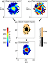 |
Fig. B.1. Output for MaNGA plate-IFU: 8244-3702. Final W80 map (bottom plot) combined from the W80 map of each model (top plots) based on the best |

Appendix C: Binning parameters
We show how the ionized gas kinematics from the [O III] emission-line (traced by the central W80 averaged over an aperture of 0.5 Reff) changes (for different galaxy populations) when observed in different parameter spaces of host galaxy properties. This is shown in Figs. A1.C.2 and A1.C.1. When looking at SF galaxies, in most cases, there is no significant evolution in their W80. Conversely, in the case of AGN-selected galaxies, stronger W80 values are found as we move to a specific direction of the parameter spaces. This is visually represented in Fig. A1.C.1, where minimal gradients are observed for SF galaxies, whereas AGN-selected galaxies show not only larger gradients but also a distinct trend toward increased stellar mass (M⋆) and L[O III] luminosity.
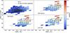 |
Fig. C.1. Average W80 binned on a plane of M⋆ vs. L[O III]. The bins have a size of 0.3 dex in each parameter, colored by the strength of the W80. The scatter dots show the distribution of a specific galaxy population and the line shows a 1D polynomial fitted to the location of the SF galaxies. The green arrows in the plots illustrate the gradient change of W80 in the parameter space, with the arrowhead indicating the direction and the arrow’s size representing the magnitude. |
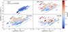 |
Fig. C.2. Average W80 binned on a plane of star formation rate measured from Lrad and LHα. The bins have a size of 0.3 dex in each parameter, colored by the strength of the W80. The scatter dots show the distribution of a specific galaxy population and the line shows the 1-to-1 relation if both SFR tracers are equal. |
All Tables
Coincident targets between the different AGN-selection techniques in the full MaNGA sample.
Coincident targets between the different AGN-selection techniques in a sample of MaNGA targets limited by S/N.
All Figures
|
Fig. 1. Definition of the radio-selected AGN candidates. We plot on the y axis the expected SFR that one would measure, assuming that all the radio luminosity can be attributed to star formation processes (SFR(Lrad); see Sect. 2.2.4). Similarly, on the x axis, the SFR is expected from Hα luminosity (SFR(Hα)). The black line corresponds to the location where SFR(Lrad) = SFR(Hα). The other colored lines (orange, red, and blue) correspond to our SFR excess definition in SFR(Hα) steps of 0.5, 1.0, and 1.5 dex (log(xi)). We defined each sample of AGN-selected candidates by selecting the targets whose values (and error bars) are above the corresponding line (following SFR(Lrad)/SFR(Hα) = xi) and we have colored them according to the colored lines (except for xi = 0.0 dex, which corresponds to the yellow ones). We also show targets that did not satisfy any SFR-excess criteria (gray without marker) or did not pass the S/N criteria (gray with marker) for our kinematic analysis (see Sect. 3.2). The contours (dashed blue, light blue, and teal) represent the density where specific galaxy populations gather (SF, composite, non-radio-selected AGNs). The top and right-hand plots show the individual parameter distribution of these three galaxy populations. |
| In the text | |
|
Fig. 2. Optical diagnostic diagrams for MaNGA galaxies. The black circles in the scatterplot show the emission-line ratio values for all MaNGA galaxies. In colored shapes, we feature the different AGN-selected candidates (see the legend). We took the flux ratio values from the ones measured around their central 2 kpc region (Albán & Wylezalek 2023). In the top panel, the gray line corresponds to the demarcation line from Kauffmann et al. (2003), and the black line (both in the top and bottom plots) corresponds to the ones from Kewley et al. (2001). |
| In the text | |
|
Fig. 3. Stellar mass versus star formation rates of MaNGA host galaxies. The left panel shows the impact of our quality criteria (see Sect. 3.2), excluding galaxies with higher stellar mass and lower star formation rates (represented by the black dots in the scatter plot and hatched black distribution in the top and right-hand diagrams). In red, orange, and yellow, we show the distribution of the AGN candidates selected by radio (using 0.0, 0.5, and 1.0 dex of excess; see Sect. 2.2.4) that satisfy the S/N quality criteria. To understand the properties of the excluded radio-selected hosts, we encourage the reader to look at Fig. 1. It can be seen that a long tail of deficient SFR hosts are excluded (−2> log(SFR(Hα)) > −4). On the right, we show only the galaxies chosen after the quality criteria and their corresponding AGN classifications. We have provided labels for each color in a panel between both plots. |
| In the text | |
|
Fig. 4. Smooth histograms of multiple host galaxy properties. Top (left to right): b/a axis ratio, log(M⋆), and log(SFR) from Pipe3D. Bottom (left and middle plot): log(L[O III]) and log(EW(Hα)), both extracted from an aperture of 1 Reff, and (to the right) a complementary illustration for Table 2 employing Venn diagrams. In order to maintain visual clarity, the hard X-ray-selected AGN sample was intentionally omitted from the diagrams. The gray-shaded histogram shows the distribution of all MaNGA that pass our S/N criteria (see Sect. 3.2). |
| In the text | |
|
Fig. 5. W80 stacked radial profiles for various galaxy groups. In the upper central panel, the colors represent these groups: black, gray, and blue for all MaNGA galaxies, non-AGNs, and SF galaxies (selected by BPT), while the remaining colors denote AGN-selected candidates. Each line in the plots represents the median value at each Reff ring, with shaded areas indicating the 14th to 86th percentiles. The leftmost plot displays unshaded profiles for easier comparison. Different line styles are used for visual clarity. |
| In the text | |
|
Fig. 6. Comparison of stacked W80 profiles and host galaxy properties between non-AGNs and optical AGNs. In each plot, blue corresponds to the behavior of a specific parameter for optically selected AGNs and black for non-AGNs. We show the W80 stacked radial profile, the log(M⋆) distribution, the log(L[O III]) distribution, and the log(SFR(Hα)) distribution. For this comparison, only log(M⋆), redshift, and morphology were controlled. |
| In the text | |
|
Fig. 7. Comparison of stacked W80 profiles and host galaxy properties between non-AGNs and sample A. In each plot, blue corresponds to the behavior of a specific parameter for sample A (see Sect. 4.1) and black for non-AGNs. For each column of plots, from left to right, we show the W80 stacked radial profile, the log(M⋆) distribution, the log(L[O III]) distribution, and the log(SFR(Hα)) distribution. The plots in the bottom row show how both samples behave after they are matched to have the same log(M⋆) and log(L[O III]). The plots in the top row show how both samples behave if the matching is done only for log(M⋆). The Venn diagrams shown in each W80 plot represent sample A. The discrepancy in the Venn diagram numbers in sample A arises from the incorporation of L[O III] into the control. |
| In the text | |
|
Fig. 8. Comparison of stacked W80 profiles and host galaxy properties between non-AGNs and sample B. Same as Fig. 7 but comparing non-AGNs (black) to sample B (blue). |
| In the text | |
|
Fig. 9. Comparison of stacked W80 profiles and host galaxy properties between different AGN samples. The plots in the top and bottom rows show how both samples behave after they are matched to have the same log(M⋆) and log(L[O III]). The Venn diagrams shown in each W80 plot represent the AGN sample in the label. Top: Blue for optically selected (without broad-line-selected) and gray for the opposite. Bottom: Blue for sample B and gray for sample A. For each column of plots, from left to right, we show the W80 stacked radial profile, the log(M⋆) distribution, the log(L[O III]) distribution, and the log(SFR(Hα)) distribution. |
| In the text | |
|
Fig. B.1. Output for MaNGA plate-IFU: 8244-3702. Final W80 map (bottom plot) combined from the W80 map of each model (top plots) based on the best |
| In the text | |
|
Fig. C.1. Average W80 binned on a plane of M⋆ vs. L[O III]. The bins have a size of 0.3 dex in each parameter, colored by the strength of the W80. The scatter dots show the distribution of a specific galaxy population and the line shows a 1D polynomial fitted to the location of the SF galaxies. The green arrows in the plots illustrate the gradient change of W80 in the parameter space, with the arrowhead indicating the direction and the arrow’s size representing the magnitude. |
| In the text | |
|
Fig. C.2. Average W80 binned on a plane of star formation rate measured from Lrad and LHα. The bins have a size of 0.3 dex in each parameter, colored by the strength of the W80. The scatter dots show the distribution of a specific galaxy population and the line shows the 1-to-1 relation if both SFR tracers are equal. |
| In the text | |
Current usage metrics show cumulative count of Article Views (full-text article views including HTML views, PDF and ePub downloads, according to the available data) and Abstracts Views on Vision4Press platform.
Data correspond to usage on the plateform after 2015. The current usage metrics is available 48-96 hours after online publication and is updated daily on week days.
Initial download of the metrics may take a while.