| Issue |
A&A
Volume 698, June 2025
|
|
|---|---|---|
| Article Number | A99 | |
| Number of page(s) | 16 | |
| Section | Extragalactic astronomy | |
| DOI | https://doi.org/10.1051/0004-6361/202453307 | |
| Published online | 03 June 2025 | |
Feedback from low-to-moderate-luminosity radio-active galactic nuclei with MaNGA
Astronomisches Rechen-Institut, Zentrum für Astronomie der Universität Heidelberg, Münchhofstr. 12-14, 69120 Heidelberg, Germany
⋆ Corresponding author: This email address is being protected from spambots. You need JavaScript enabled to view it.
Received:
4
December
2024
Accepted:
23
March
2025
Abstract
Context. Spatially resolved spectral studies of galaxies hosting a radio-active galactic nucleus (radio-AGN) have shown that these systems can impact ionised gas on galactic scales. However, it is still unclear whether jet and radiation-driven feedback occurs simultaneously. The relative contribution of these two mechanisms in driving feedback in the AGN residing in the Local Universe is also poorly understood.
Aims. We selected a large and representative sample of 806 radio-AGN from the MaNGA survey, which provides integral field unit (IFU) optical spectra for nearby galaxies. We define radio-AGN as sources having excess emission above the level that is expected from star formation. We aim to study the feedback driven by radio-AGN on the galaxy’s ionised gas, its location, and its relation to AGN properties. We also aim to disentangle the role of jets and radiation in these systems.
Methods. We used a sample of nearby radio-AGN from L1.4 GHz ≈ 1021 − 1025 W Hz−1 to trace the kinematics of the warm ionised gas phase using their [O III] emission line. We measured the [O III] line width and compared it to the stellar velocity dispersion to determine the presence and location of the disturbed gas. We investigated the dependence of radial profiles of these properties on the presence of jets and radiation, along with their radio luminosities.
Results. We mainly found disturbed [O III] kinematics and proportion of disturbed sources up to a radial distance of 0.25 Reff, when both radio- and optical-AGN are present in a source, and when the radio luminosity is greater than 1023 W Hz−1. When it is either only radio- or optical-AGN present, the impact on [O III] is milder. Irrespective of luminosity and the presence of an AGN, we find no evidence for feedback from radio-AGN on [O III] kinematics at radial distances larger than 0.25 Reff.
Conclusions. The presence of more kinematically disturbed warm ionised gas in the central region of radio-AGN host galaxies is related to both jets and radiation in these sources. We propose that in moderate-radio-luminosity AGN (L1.4 GHz ≈ 1023 − 1025 W Hz−1), the gas clouds pushed to high velocities by the jets (radiation) are driven to even higher velocities by the impact of radiation (jets) when both radio- and optical-AGN are present. At lower luminosities (L1.4 GHz ≈ 1021 − 1023 W Hz−1), the correlation between the disturbed ionised gas and enhanced radio emission could either be due to wind-driven shocks powering the radio emission or low-power jets disturbing the gas. Finally, beyond 0.25 Reff, the lack of any disturbed [O III] suggests a weak coupling between the jets and the ionised gas in these sources.
Key words: galaxies: active / galaxies: evolution / galaxies: jets / galaxies: kinematics and dynamics
© The Authors 2025
 Open Access article, published by EDP Sciences, under the terms of the Creative Commons Attribution License (https://creativecommons.org/licenses/by/4.0), which permits unrestricted use, distribution, and reproduction in any medium, provided the original work is properly cited.
This article is published in open access under the Subscribe to Open model. This email address is being protected from spambots. You need JavaScript enabled to view it. to support open access publication.
1. Introduction
Feedback from active galactic nuclei (AGN) is a critical component of models of galaxy evolution. A fraction of the energy released during an AGN phase can couple with the gas of the host galaxy, preventing it from forming stars. This kind of negative feedback is used to explain the cessation of star formation in massive galaxies that would otherwise be too large and too massive (e.g. Silk & Rees 1998; Di Matteo et al. 2005; Fabian 2012). The radiative and mechanical energy required for this feedback can be carried by accretion-driven winds, radiation pressure, collimated jets of plasma, and other effects (see King & Pounds 2015; Harrison & Ramos Almeida 2024 for a review).
On intergalactic scales, the released energy can prevent the cooling and eventual accretion of gas from the hot halos surrounding galaxies, which fuels star formation (McNamara & Nulsen 2012, 2007). On galactic scales, AGN-driven feedback can shock the gas clouds, making them turbulent and sometimes even pushing them to high velocities (outflows). This prevents the gas clouds from collapsing to form stars. These processes occur on different physical scales and timescales, therefore, an understanding of how AGN interact with their host galaxies is crucial. Over the past few years, many studies have found evidence for negative feedback on galactic scales, attributed to both radiatively efficient and inefficient AGN (e.g. Venturi et al. 2021; Speranza et al. 2021; Morganti 2021; Murthy et al. 2019).
Statistical studies of large samples have found a positive correlation between the presence of an AGN and its energy output, as well as the presence of kinematically disturbed gas (e.g. Mullaney et al. 2013; Woo et al. 2017; Santoro et al. 2020; Kukreti & Morganti 2024), albeit with spatially unresolved spectra. Although it is useful to understand the population as a whole, these unresolved spectra cannot provide information about the location of the disturbed gas or the affected stellar population in the galaxy. This spatial information is needed to understand the scales of AGN-driven feedback occurring in galaxies.
Spatially resolved spectra from an integral field unit (IFU) can provide information about the gas and stellar emission at different locations in the host galaxy. This has led to the discovery of a number of trends between the spatial distribution of the disturbed gas and the energy released by the AGN. For example, a positive correlation between the size of the kinematically disturbed ionised gas region and the radiative luminosity has been found for AGN with radiatively efficient accretion (Seyferts, Quasars; e.g. Kang & Woo 2018; Kim et al. 2023; Gatto et al. 2024). For similar sources, positive correlations have also been found between the width of the emission line profiles tracing the disturbed gas and the radiative luminosity (e.g. Wylezalek et al. 2020; Deconto-Machado et al. 2022). This illustrates the role of radiation in driving feedback in AGN host galaxies. However, such systematic spatially resolved studies in radiatively inefficient AGN where jets are prominent have rarely been conducted. It is important to study feedback in sources where both the jets and radiation from the AGN are present, so that we can understand the role and relative contributions of these two mechanisms.
Studying feedback in radio-AGN hosts can help us gain key insights in this direction. In this paper, we define radio-AGN as sources with excess radio emission above the level expected from star formation. However, we note that the definition is not uniform across the literature. Although the excess radio emission in radio-AGN is often due to collimated plasma jets launched during the active phase, in some low-luminosity sources, it can also originate from shock interactions between AGN-driven winds and the interstellar medium (ISM; Zakamska et al. 2016), relating the radio emission to the radiative output of the AGN. A large fraction of radio-AGN have radiatively inefficient accretion, but a significant proportion also show radiatively efficient accretion. This makes them ideal for improving our understanding of the role of the mechanical and radiative energy output of an AGN.
Many studies have found observational evidence for jet-driven feedback on the ionised gas in these galaxies using IFU data. However, these studies have mostly been focused on single objects or small samples (e.g. Jarvis et al. 2019, 2021; Cresci et al. 2023; Girdhar et al. 2022; Speranza et al. 2021; Nesvadba et al. 2021; Ruffa et al. 2022; Riffel et al. 2023a; Ulivi et al. 2024; Venturi et al. 2021). Studies of large samples of radio-AGN with spatially resolved spectra have been challenging to perform due to the lack of IFU data for a large sample of galaxies. This can now be achieved with the Mapping Nearby Galaxies at APO (MaNGA) survey (SDSS-IV), which is the largest IFU survey till date, covering a sample of ∼10 000 galaxies over a redshift range of 0.01 < z < 0.15. This survey provides spatially resolved spectra from 3600−10 300 Å, which covers emission lines such as [O III], Hβ, Hα, [N II], and others that can serve as good indicators of AGN interaction and ionisation. Recently, Albán et al. (2024) identified AGN in MaNGA using multi-wavelength data and they studied the warm ionised gas kinematics using the [O III] line. They found evidence for enhanced ionised gas kinematics over galactic scales for radio-AGN compared to optical-AGN, suggesting that radio-AGN might be tracing AGN at an advanced stage of the activity and feedback cycle.
We use the MaNGA survey data to study feedback from radio-AGN on the host galaxy’s warm ionised gas (T ∼ 104 K), using the [O III]λλ4958, 5007 Å doublet as a tracer. We use two radio surveys: the LOFAR Two-metre Sky Survey at 144 MHz (LoTSS; Shimwell et al. 2017, 2022) and the Faint Images of the Radio Sky at Twenty-cm survey at 1400 MHz (FIRST; Becker et al. 1995) to identify the largest sample of radio-AGN from MaNGA. We trace the ionised gas using the [O III] emission line and determine the physical scales on which the radio-AGN impacts it. Our main aim is to disentangle the role of jets and radiation in driving feedback on warm ionised gas and determine the impact of these two mechanisms when they are present in the same source. The large size of these three surveys, combined with the high sensitivity of LoTSS to faint radio emission, allows us to cover a large range of radio luminosities from L1.4 GHz ≈ 1021 − 1025 W Hz−1. This makes the sample a good representative of the radio-AGN population in the Local Universe and ideal for investigating and understanding their potential feedback mechanisms.
This paper is structured as follows. Section 2 describes the sample construction and selection of radio-AGN. Section 3 describes the modelling of the stellar continuum and emission line profiles of the sources. We present the results for different source groups in Sect. 4, discuss them in Sect. 5 and summarise our results in Sect. 6. Throughout the paper, we use the ΛCDM cosmological model, with H0 = 70 km s−1 Mpc−1, ΩM = 0.3, and Ωvac = 0.7.
2. Sample construction
This section outlines the approach used to select the radio-AGN, optical-AGN, and control sample of non-AGN. The MaNGA survey provides a wavelength coverage over 3600−10 300 Å with a spectral resolution of R ∼ 2000, corresponding to a spectral line-spread function width of about 70 km s−1 (1σ). The IFU field of view diameter varies from 12″ to 32″. For more details on the survey, we refer to Bundy et al. (2015). The data reduction was performed using the MaNGA Data Reduction Pipeline (DRP), described in Law et al. (2016, 2021). Next, the spectral fitting was done using the MaNGA data-analysis pipeline (DAP) described in Westfall et al. (2019), which fits the stellar continuum and emission lines to the entire spectrum. Since this paper is focussed on the [O III] gas kinematics, we used the emission line-only spectra from the DAP, obtained after subtracting the stellar continuum from the reduced observed spectra. Sánchez et al. (2022) constructed a catalogue of the host galaxy properties from a spectral analysis using the pyPipe3D pipeline (Lacerda et al. 2022). We used the stellar mass, effective radius, and ellipticity properties from their value-added catalogue.
Furthermore, we removed duplicate observations from the catalogue. Albán et al. (2024) carried out a careful inspection of the MaNGA data and identified new duplicate observations, then combined them with the already known duplicates from Sánchez et al. (2022) and the survey website1. They also removed sources flagged CRITICAL in the MANGA_DRP3QUAL column of the DRP table. Finally, this gave us a sample of 9777 sources.
Selecting a large sample of radio-AGN from MaNGA is important to obtain statistically reliable results. LoTSS has high sensitivity and source density, whereas FIRST has a larger area overlap with MaNGA. LoTSS and FIRST have 56% and 97% sky area overlap with MaNGA, respectively. Therefore, we used both surveys to maximise the number of radio cross-matches. We cross-matched the MaNGA sample with the LoTSS DR2 (6″ angular resolution) and FIRST (5.4″ angular resolution) catalogue using Topcat (Taylor 2005), with a 6″ radius, which is equal to LoTSS and close to FIRST resolution. We cross-matched the sample down to flux densities of 0.3 mJy in LoTSS and 0.5 mJy in FIRST, to ensure that the detections have a S/N > 3. This limit is chosen to maximise the number of cross-matches with MaNGA, while keeping only reliable detections. At a search radius of 6″, we determined a contamination level from false-positive matches of ∼2.5% for LoTSS cross-matches and 0.7% for FIRST cross-matches (Galvin et al. 2020). We found cross-matches for 2493 sources in LoTSS and 1155 sources in FIRST. LoTSS is sensitive to extended emission around sources and therefore provides a reliable measurement of the total flux density at 144 MHz. However, FIRST has poor sensitivity to extended emission, meaning it could underestimate the total flux density at 1.4 GHz. For more reliable estimates of the total flux density at 1.4 GHz, we used the combined radio catalogue from Mingo et al. (2016), which cross-matched the FIRST and NRAO VLA Sky Survey (NVSS; Condon et al. 1998). They used the flux densities from the lower resolution (∼45″) NVSS survey, which recovers the total flux better than FIRST. Finally, we used the 144 MHz and 1.4 GHz total flux densities to estimate the k-corrected total radio luminosities, L144 MHz and L1.4 GHz.
The diagnostics we used to select radio-AGN were constructed and optimised using the value-added spectroscopic catalogues produced by the group from the Max Planck Institute for Astrophysics, and The Johns Hopkins University (MPA-JHU; Brinchmann et al. 2004). These include galaxy parameters measured using single fibre spectra from SDSS DR8. Since we used these diagnostics for radio-AGN selection, we used the MPA-JHU catalogue measurements for our galaxies, which include the Dn(4000), [O III], Hβ, [N II], and Hα fluxes. Using a matching radius of 6″, we found cross-matches for 9072 sources in our sample. Since this cross-match missed some MaNGA sources, we also used the Sánchez et al. (2022) value-added catalogue, which provides these measurements using a 2.5″ aperture (similar in size to the SDSS fibre). Although we did not use the Sánchez et al. (2022) catalogue measurements for all the sources, we note that using the 2.5″ aperture values for the entire sample only leads to a small fraction of sources being classified differently, but does not change our results.
In one of the diagnostics discussed in Sect. 2.1, we used mid-infrared (MIR) colours to separate star-forming and passive sources. For this, we used Wide-field Infrared Survey Explorer (WISE) data from the allWISE IPAC release (November 2013; Cutri et al. 2021). This provides magnitudes in three bands: W1 at 3.4 μm, W2 at 4.6 μm, and W3 at 12 μm, with an angular resolution of 6.1 − 6.5″. To obtain reliable detections, we only selected sources with cc_flag = 000, as suggested in the online user manual. We used a signal-to-noise ratio (S/N) threshold of 5 for W1 and W2 and 3 for W3 (due to its poorer sensitivity). With these criteria, we obtained a WISE cross-match for 7616 sources.
Finally, we aimed to construct radial profiles of [O III] line widths to study the spatial changes in [O III] kinematics. Galaxy morphology is an important property that can affect the gravitational motion of the gas and, thus, the spatial distribution of the [O III] line widths as well. This distribution can change depending on the relative strength of the bulge or disk component. To control for this, we added morphological classifications of the MaNGA galaxies from the Deep Learning DR17 Morphology catalogue (Domínguez Sánchez et al. 2022; Fischer et al. 2019). We used the T-Type parameter for this purpose. Broadly, galaxies with T-Type < 0 are ellipticals, T-Type ∼0 are S0s, and T-Type > 0 are late types. We controlled the T-Type distribution of the different groups studied in Sect. 4 to ensure that the effect of morphology is not driving the trends that we have observed.
2.1. Selecting radio-AGN
In the Local Universe, star-forming galaxies (SFGs) dominate a radio-selected sample up to L1.4 GHz ≈ 1023 W Hz−1 (Sadler et al. 2002; Best et al. 2005). Most MaNGA sources with a radio cross-match have a luminosity lower than this value. Therefore, we first need to select a clean sample of radio-AGN, namely, sources where radio emission exceeds that expected from star formation and can be attributed to the AGN in the galaxy. To this end, we use a combination of four diagnostics created by Best et al. (2005), Best & Heckman (2012) and further developed by Sabater et al. (2019). We point to these references for a detailed discussion of these methods. We first selected radio-AGN from the LoTSS cross-matched sample using diagnostics shown in Fig. 1 and then from the FIRST cross-matched sample using the diagnostics shown in Fig. A.1.
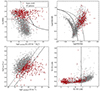 |
Fig. 1. Diagnostic plots for selecting radio-AGN using LoTSS data. Red points mark the sources classified as radio-AGN after combining all four diagnostics, and grey points show the star-forming/radio-quiet AGN: (a) Dn(4000) vs L1.4 GHz/M⋆ plot. The solid and dashed curves mark the radio-AGN, intermediate and SF/RQAGN division from Best & Heckman (2012) and Sabater et al. (2019); (b) LHα versus L1.4 GHz plot, with the separation lines from Sabater et al. (2019); (c) BPT diagram where the solid curve shows the semi-empirical relation from Kauffmann et al. (2003), and the dashed curve shows the maximum starburst curve from Kewley et al. (2006); (d) WISE colour-colour plot for sources with the division line from Sabater et al. (2019). |
The first diagnostic is the ‘Dn(4000) versus Lradio/M⋆’ method. Here, Dn(4000) is the spectral break at 4000 Å, which is an indicator of the mean stellar age, while Lradio/M⋆ is the ratio of radio luminosity and stellar mass. These quantities depend on the star formation rate of a galaxy and can be used to locate SFGs on a plane. Best et al. (2005) showed that SFGs broadly occupy the same region on a plot of these two quantities for a large variety of star formation histories. But in the case of radio-AGN, excess radio emission from the AGN would increase the Lradio/M⋆ value, separating them from the SFGs. Based on this idea, Best et al. (2005) and Kauffmann et al. (2008) obtained a track to separate SFGs from radio-AGN. Sabater et al. (2019) selected radio-AGN from LoTSS-DR1 and added another track that follows the original track till Dn(4000) = 1.7, then continues horizontally. They helped maximise agreement with the more sophisticated selection of SFGs by Gürkan et al. (2018) for the H-ATLAS sample and select low-luminosity radio-AGN that have high Dn(4000) values. Since MaNGA sources typically have low radio luminosities, we also used the track of Sabater et al. (2019)2. For Lradio, we used the 144 MHz and 1.4 GHz luminosity, respectively, for LoTSS and FIRST cross-matched sources. For FIRST cross-matched sources, we scaled the diagnostic tracks to 1.4 GHz, assuming an optically thin spectrum modelled as S ∝ να, with a spectral index of α = −0.7. Varying α between −0.5 and −1 does the change the classification of a few sources, but does not affect our results. In the ‘Dn(4000) versus Lradio/M⋆’ plot in Figs. 1 and A.1, sources above the solid line are classified as radio-AGN, sources below the dashed line are classified as SFGs and sources between the two lines are classified as intermediate.
The second diagnostic is the LHα versus Lradio plot. The star formation rate of massive stars can determine both Hα and radio luminosities of galaxies. Therefore, sources with excess radio emission contribution from an AGN can be separated on a plot of these two properties. We again use the relations from Sabater et al. (2019) for the 144 MHz luminosity of LoTSS cross-matched sources: log(LHα/L⊙) = log(L144 MHz/W Hz−1)−16.1 and log(LHα/L⊙) = log(L144 MHz/W Hz−1)−16.9. These relations were derived to again maximise the agreement with the results of Gürkan et al. (2018) for the H-ATLAS sample to avoid any misclassification of low-luminosity sources. In the plots shown in Figs. 1 and A.1, sources with less LHα than the lower line are classified as radio-AGN, sources between the two lines as intermediate and above the upper line are classified as star-forming. We used Hα non-detections in cases where they provided useful upper limits on LHα. For FIRST cross-matched sources, we scaled the relations mentioned above to 1.4 GHz and performed the same classification.
The third diagnostic used is the BPT diagram, where we use the [N II]/Hα and [O III]/Hβ emission line ratios to separate sources ionised by AGN or star-formation. We used the division from Kauffmann et al. (2003) and the maximum starburst relation form Kewley et al. (2006). Sources with larger ratios than the maximum starburst curve were classified as AGN, between the two curves as intermediate and below the lower curve as star-forming. Although this does not use any radio property, it can still give information about the presence of AGN or star formation in the source. Again, we used non-detections in cases where they provided useful upper limits.
The final diagnostic is the WISE colour-colour diagram, between the W1 − W2 and W2 − W3 colours. Radio-AGN host galaxies are typically ellipticals, with low levels of star formation. These can be separated from star-forming galaxies based on their W2 − W3 colour (Yan et al. 2013). Sabater et al. (2019) modified the division of Herpich et al. (2016) based on comparison with the results of Gürkan et al. (2018) for the H-ATLAS field as mentioned before. We used their division of W2 − W3 (AB) = 0.8.
We classified the LoTSS and FIRST cross-matched sources independently. This was done to maximise the number of radio-AGN selected from the sample. In each diagnostic (except the WISE diagram), a source can be labelled as radio-AGN, intermediate, star-forming, or unclassified. This gives a total of 192 possible combinations. These combinations are used to give a final classification, following the approach of Sabater et al. (2019) and Best & Heckman (2012). This approach gives the most weight in classification to the ‘Dn(4000) versus Lradio/M⋆’ and ‘LHα versus Lradio’ diagnostic. Sources classified by either of these plots as an AGN are classified as a radio-AGN in the final classification. The BPT and WISE colour-colour diagnostics have the least weight (as they have no radio information) and are used only when the first two diagnostics give inconclusive classifications. Their main purpose at this stage is to check whether a source is hosting SF or not. For example, if both of the first two radio diagnostics classify a source as ‘intermediate’, we used the BPT and WISE colour-colour plot to check if the source lies in the SF region to determine whether the radio emission can be explained by SF. It is worth noting that the main aim of this selection technique is to select a clean sample of radio-AGN and is not necessarily complete, as it might miss some radio-AGN that reside in SF galaxies.
The different combinations of the diagnostics, the number of sources in each group and the final classification are summarised in Table 1 for LoTSS sources and Table A.1 for FIRST sources. The number of sources classified in each diagnostic and the final number of radio-AGN from LoTSS and FIRST cross-matches, are summarised in Tables 2 and A.2, respectively. Finally, we select 499 LoTSS and 512 FIRST sources as radio-AGN, which leads to a combined sample of 806 radio-AGN identified either with LoTSS or FIRST. Of these, 205 are common in both LoTSS and FIRST samples, 294 are unique in LoTSS, and 307 are unique in the FIRST radio-AGN sample. For radio-AGN with only a LoTSS detection, we estimated the k-corrected 1.4 GHz luminosity by extrapolating the flux from 144 MHz using a power law of the form Fν ∝ να, with a spectral index α = −0.7. This allows us to assess them together with radio-AGN that have FIRST detections. The distribution of this radio-AGN sample on the L1.4 GHz versus L[O III] plot is shown in Fig. 2.
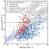 |
Fig. 2. 1.4 GHz and [O III] luminosities of the sources with an [O III] detection. Sources with radio+optical AGN, radio-AGN, and optical-AGN are shown. For optical-AGN without a radio detection, the arrows show the upper limits on L1.4 GHz. The shaded regions show the expected radio luminosity from the shocks scenario using the Nims et al. (2015) model, where the lower and upper edges show the limits for 5% and 25% coupling efficiency between AGN luminosity and wind kinetic luminosity, respectively. Different regions show the [O III] to bolometric luminosity conversion factors from Heckman et al. (2004) and Stasińska et al. (2025). The horizontal dotted lines show the luminosity divisions used in Sect. 4. To highlight the low-to-moderate luminosity nature of the sources in our study, we also show the parameter space occupied by the radio-AGN sample from Kukreti & Morganti (2024) in black contours, which examines the relation between radio properties and feedback on [O III] out to z = 0.8. |
Diagnostic combinations for LoTSS sources.
Classification of LoTSS cross-matched sources.
Our radio-AGN sample mostly covers a L1.4 GHz range of ≈1021 − 1024 W Hz−1, with the majority of sources below 1023 W Hz−1, which can be classified as low-luminosity radio-AGN. Over the past years, studies of feedback in radio-AGN host galaxies with IFU data have mostly focused on moderate to high luminosity (≳1025 W Hz−1) radio-AGN, as discussed in the Introduction. However, with the combination of large IFU surveys like MaNGA and sensitive radio surveys like LoTSS, it is now possible to perform such studies for low-to-moderate luminosity radio-AGN, which make up the majority of the radio-AGN population in the Local Universe (Best et al. 2005; Sadler et al. 2002; Sabater et al. 2019). Therefore, our study of mostly low-luminosity radio-AGN can help us understand the role of this population in driving feedback. The low-luminosity nature of our sample is highlighted in Fig. 2, where we also show the sample from Kukreti & Morganti (2024) for comparison. Radio-AGN in this sample were selected using the same diagnostics to study feedback on [O III] up to z = 0.8 using single fibre SDSS spectra.
Although the radio emission in radio-loud AGN is attributed to jets of relativistic plasma, the origin is less clear for radio-quiet AGN. One interesting explanation for radio emission in these sources is the shock scenario. This includes radiatively accelerated winds driving shocks into the host galaxy medium, which accelerate particles that then produce synchrotron emission (Faucher-Giguère & Quataert 2012; Zakamska & Greene 2014; Zakamska et al. 2016; Zubovas & King 2012). This scenario can explain the origin of radio-emission in low-to-moderate radio-luminosity sources, similar to the ones in our sample. In Fig. 2, we also show the expected shock-generated radio luminosities from the fiducial models of Nims et al. (2015). This model estimates the expected radio luminosity for a certain AGN bolometric luminosity. However, there are significant uncertainties in the coupling efficiencies between the AGN bolometric luminosity, wind kinetic luminosity, and energy of the accelerated electrons. The conversions determining the bolometric luminosity from the observed [O III] luminosity are also uncertain. We show the Nims et al. (2015) model for two different conversions of [O III] to bolometric luminosity, from Heckman et al. (2004) and Stasińska et al. (2025), covering a range of coupling efficiencies. We find that ∼40% of the sources with radio+optical AGN (Sect. 2.3) lie beyond the radio luminosity limit of this model and very likely have radio emission dominated by jets. In the rest, the radio emission could also be due to shocks. We discuss this further in Sect. 5.
2.2. Other MaNGA radio-AGN catalogues
Multiple studies in the literature have selected radio-AGN samples from the MaNGA catalogue and we compare those samples to our own in this work. Comerford et al. (2024) cross-matched the MaNGA catalogue with the radio-AGN catalogue of Best & Heckman (2012), which was itself selected using the SDSS DR7 source catalogue with the FIRST and NVSS surveys. They found 221 of these radio-AGN in the MaNGA catalogue. We cross-matched the Best & Heckman (2012) catalogue with our 9777 MaNGA sources using a 6″ match radius and found 214 radio-AGN instead. The discrepancy could be due to the different number of MaNGA sources used to start with. Out of these 214 sources, 199 were selected as radio-AGN by our selection criteria with FIRST data. Of the remaining 15 sources, 13 do not have a cross-match in FIRST in our sample, likely due to a difference in the cross-matching criteria from Best & Heckman (2012); the remaining 2 sources have a FIRST crossmatch but are not classified as radio-AGN in our sample. Although our selection criteria are based on Best & Heckman (2012), we used the modified selection criteria by Sabater et al. (2019), which attempt to include more low-luminosity radio-AGN misclassified as SF before. We also select sources below the 5 mJy threshold used by Best & Heckman (2012), which would explain the larger number of radio-AGN we identified compared to Comerford et al. (2024). Broadly, almost all the radio-AGN in the Comerford et al. (2024) sample are included in ours.
A sample of 307 radio-AGN has also been selected from MaNGA by Mulcahey et al. (2022) using the same diagnostics as we use and LoTSS DR2 data. Compared to the radio-AGN selected using LoTSS data in our sample, we find an overlap of 189 sources. The sources that do not overlap are among the low-luminosity (L144 MHz ≈ 1021 − 1023 W Hz−1) sources in our sample. We found that the radio luminosities in that study have been overestimated, which could affect the classification and explain this discrepancy. However, this does not affect the results of that study3.
Recently, Albán et al. (2024) also selected a sample of 288 radio-AGN from the MaNGA catalogue with a [O III] S/N > 7, by comparing the star formation rates (SFRs) estimated from 1.4 GHz (FIRST+NVSS) and Hα luminosities (obtained from Sánchez et al. 2022 catalogue). On a plot of the two SFRs, they selected sources with a radio SFR more than 0.5 dex away from the 1:1 relation. Out of their 288 sources, 97 are also classified as radio-AGN in our sample using FIRST, and 159 are classified as SF/radio-quiet. This discrepancy is due to the significantly different selection methods and the different FIRST detection threshold they use of 1 mJy. Indeed, most of the disagreeing sources in the two samples lie close to the 0.5 dex division line on the SFR plot of Albán et al. (2024). Thirty sources in their sample do not have a FIRST crossmatch in our sample. This discrepancy is because they also cross-match with the NVSS catalogue, which gives them more sources with a radio detection at 1.4 GHz. We compare and discuss the Albán et al. (2024) catalogue in more detail in Sect. 5, since these authors also measured the radial profiles of the [O III] line width. Recently, Suresh & Blanton (2024) also selected a sample of radio-AGN using a similar approach of comparing radio and Hα based SFRs, but used a 1 dex threshold from the 1:1 line.
2.3. Optical-AGN sample
Since we are aiming to understand the complementary roles of jets and radiation in driving feedback, we also constructed a sample of optical-AGN using the BPT classification in Sect. 2.1. We first identified all sources with an AGN classification in the BPT diagram. We then selected only those sources with an Hα equivalent width greater than 3 Å. This was done to ensure that the ionisation is due to an AGN in these sources, as Cid Fernandes et al. (2010, 2011) showed that sources with weaker Hα emission that lie in the AGN (LINER) region of the BPT diagram, can have ionisation from hot low mass evolved stars, instead of an AGN. This gives us a sample of 482 optical-AGN, out of which 73 are also classified as radio-AGN. We therefore have 409 sources that are optical-AGN. We note that an optical-AGN sample using MaNGA data was also selected by Albán & Wylezalek (2023) using different aperture sizes. We find that 369 of our optical-AGN sources are also classified as AGN in their study. However, 113 of our sources are not classified as an AGN in their selection. These sources have low S/N line detections and [O III] luminosities. Therefore, this difference is likely a result of the different data used for selection. They use a 2 kpc aperture in the central region to classify sources, whereas we use the data from the MPA-JHU catalogue, which is based on single fibre SDSS data. Since the single fibre data provides integrated fluxes over larger areas (∼2 − 8 kpc) at these redshifts, it can recover lower flux emission with higher S/N than IFU data.
Finally, we also split the radio-AGN sample into those with and without an optical-AGN, using the same criteria as above. This helps us disentangle the role of jets and radiation in Sect. 4. Out of the 806 radio-AGN selected above, 73 are also optical-AGN. For the rest of the paper, we refer to sources with both radio and optical-AGN as radio+optical AGN. Sources with either only a radio or optical-AGN are simply referred to as radio or optical-AGN.
The selection methods used above can miss radio+optical AGN that have low radio luminosities, but are optically bright. The extra contribution from AGN to the Hα luminosity, on top of any star-formation, might shift the sources vertically upwards on the LHα versus Lradio plot, into the SF region. Therefore, our selection techniques would not be able to identify the radio-AGN in these sources. This has been observed before for quasars with low radio luminosities by Jarvis et al. (2021), and would require high-resolution (sub-arcsecond) radio imaging to confirm the presence (or absence) of a radio-AGN. We note that such missed sources could contaminate our optical-AGN sample. However, the selection techniques used here still enabled us to select a clean sample of radio and radio+optical AGN.
The presence of broad emission lines from the type 1 AGN in the sample can affect the derived measurements of the host galaxy properties. We tested for any systematic bias introduced by the presence of broad-line AGN in the Dn(4000), stellar velocity dispersion and stellar mass measurements by comparing the broad-line optical (and radio+optical) AGN with the narrow-line AGN. We used the broad-line galaxy catalogue of MaNGA from Fu et al. (2023), which contains 135 galaxies. In comparing the broad-line and narrow-line AGN, we found no systematic bias in the measurements mentioned above. Thus, we conclude that this potential bias does not contaminate our radio-AGN sample selection.
2.4. Non-AGN control sample
To test whether any disturbed [O III] is associated with the presence of a radio-AGN, we also selected a control sample of non-AGN galaxies for comparison. These sources do not necessarily have radio detection. First we only selected sources classified as SF on the BPT diagram. We removed all the sources classified as radio-AGN in Sect. 2.1. Then, we removed the AGN selected using MIR data from WISE (123) and X-ray data from BAT (29), compiled by Comerford et al. (2024). Lastly, we also removed any broad-line galaxies (135) present in the catalogue of Fu et al. (2023), since these are mostly AGN as well. After visual inspection of the optical images and the [O III] maps shown in Figs. 3 and A.2, we also removed any mergers where the [O III] kinematics was affected by the interactions. We then restricted the sample to M⋆ > 1011 M⊙ and σ⋆ > 150 km s−1, to match the distributions of our radio-AGN sample. This gave us a total of 63 non-AGN sources. We estimated that the radio non-detections in the non-AGN sample have a radio luminosity value below L1.4 GHz = 3 × 10²² W Hz−1. An example of a non-AGN source is shown in Fig. A.2.
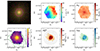 |
Fig. 3. Maps of a radio-AGN from the sample (plateifu = 8714−3704). The top left image shows the SDSS optical colour image of the host galaxy, with the MaNGA FoV marked with magenta. The other panels show the stellar and [O III] emission line properties. Only spaxels with a [O III] detection of S/N > 5 are shown and used throughout the paper for analysis. The green contours show the radio emission from FIRST at 1.4 GHz in the bottom left panel. The elliptical annuli regions used for constructing radial profiles are shown in the bottom middle panel. The same plot for a non-AGN source is shown in Fig. A.2 to illustrate the differences in their gas kinematics. |
3. [O III] spectra modelling and analysis
We went on to characterise the [O III] spectra of the MaNGA galaxies. The presence of disturbed gas kinematics is often evident in the broad low amplitude components of the emission line. This requires careful modelling of the [O III] line profile. Although the DAP catalogue provides measurements for emission lines, they used only a single component when modelling the line profiles, which is insufficient for our purpose. Therefore, we used the best-fit models from Albán et al. (2024), who fit the [O III] spectrum of each spaxel with up to two Gaussian components. They used the least-squares algorithm to fit the components to both lines in the [O III] doublet simultaneously. We refer to Sect. 3 of their paper for more details on the fitting procedure.
After determining the best-fit model, we estimated the W80 widths of the [O III] profiles. This line width encloses 80% of the total flux and is defined as the difference between the velocities that enclose 10% and 90% of the cumulative flux; namely, W80 = v90 − v10. Using W80 allows us to include emission from broad components that are likely tracing kinematically disturbed gas, while also avoiding being overly sensitive to the low S/N emission. It also enables comparison between profiles fit with different numbers of components. For a single Gaussian component, W80 is related to the velocity dispersion σ as W80 = 2.563 × σ, but the relation is not straightforward for multiple components. Using the approach outlined in Sun et al. (2017), we correct the W80 values using the instrumental spectral resolution of ≈70 km s−1 and subtract the equivalent W80 value in quadrature from the [O III] value. An example of a corrected ![Mathematical equation: $ W^{[{\mathrm{O}{\small { {\text{ III}}}}}]}_{80} $](/articles/aa/full_html/2025/06/aa53307-24/aa53307-24-eq1.gif) map for a source in our radio-AGN sample is shown in Fig. 3.
map for a source in our radio-AGN sample is shown in Fig. 3.
Next, to inspect the spatial changes in the line widths of, we constructed radial profiles of W80 using the procedure described in Albán et al. (2024), Albán & Wylezalek (2023). These profiles are constructed using elliptical annuli apertures of widths equal to 0.25 × Reff, where Reff is the galaxy’s effective radius. Using annuli widths in units of Reff makes it possible to compare the radial profiles of galaxies with different sizes. The ratio of the major and minor axis and the position angle of the elliptical aperture are set using ‘b/a’ ratio and position angle values from the value-added catalogue of Sánchez et al. (2022). Figure 3 shows a source from the sample with the elliptical annuli used. We then estimated each annuli’s pixel-weighted average W80, using the routine described in Albán et al. (2024). Furthermore, we only used galaxies with (a) at least 10 spaxels with a peak S/N > 5 detection and (b) at least two annuli with 10% area covered by spaxels with a peak S/N > 5. Although this drastically reduces the number of radio-AGN used later in our study, we used these criteria to obtain reliable radial profiles. The S/N threshold of 5 is chosen to maximise the number of sources while avoiding contamination from low S/N spectra. Changing the S/N threshold to 3 or 10 changes the number of sources with [O III] radial profiles, but it does not alter our conclusions. Out of the 806 radio-AGN selected using LoTSS and FIRST, there are 378 sources with [O III] W80 radial profiles. We removed four sources from this sample that show signs of mergers in their optical images and where the [O III] kinematics was affected by these interactions. Finally, we have a sample of 374 radio-AGN. From the control sample discussed above, we have 28 sources with [O III] radial profiles that we use for comparison with the AGN groups in Sect. 4.
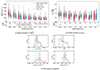 |
Fig. 4. Comparison of the four groups with: an optical and radio-AGN, radio-AGN, optical-AGN, and non-AGN. Radial profiles of |
![Mathematical equation: $ W^{[{\mathrm{O}{\small { {\text{ III}}}}}]}_{80} $](/articles/aa/full_html/2025/06/aa53307-24/aa53307-24-eq2.gif)
The line width of [O III] profiles can provide insights into the impact of AGN feedback. However, the observed width of the profiles is determined by both gravitational kinematics due to the motion of gas in the galaxy and non-gravitational kinematics due to AGN and star formation-driven feedback. It is therefore crucial to assess the contribution of both to understand the extent to which [O III] gas is disturbed. We control for this first by constraining the sample to a certain stellar mass and stellar velocity dispersion limit, as described in the next section. Furthermore, in spatially resolved maps, [O III] profiles at the central region of the galaxy can also be broad due to the blending of narrow-line profiles attributed to rotation (also depending on the inclination angle of the galaxy). This makes it hard to judge the impact of AGN solely with [O III] profile widths. We attempt to overcome this by normalising the [O III] W80 with stellar W80 values. This should (mostly) correct for the effects mentioned above since there is a broad correlation between [O III] and stellar velocity dispersions (σ⋆) observed in AGN host galaxies (e.g. Nelson & Whittle 1996; Boroson 2002; Sexton et al. 2020), and has been used before to trace AGN feedback (e.g. Woo et al. 2016; Ayubinia et al. 2023). The stellar velocity dispersions would also be affected by the gravitational potential of the galaxy and the blending effect mentioned above. Therefore, any relative differences in the [O III]/stellar W80 ratios could be due to non-gravitational kinematics, tracing AGN or star formation-driven feedback. We construct these ratio maps as described below.
We first construct maps of σ⋆, using the STELLAR_SIGMA extension in the MAPS files from the MaNGA DAP data products. We correct the stellar velocity dispersions using the STELLAR_SIGMACORR extension included in the MAPS files, and as described in the online user manual. We then convert σ⋆ to a W80 value, using a single Gaussian component conversion. Finally, we make the [O III] to stellar W80 ratio maps (only for pixels with S/N > 5 [O III] detection) defined as ![Mathematical equation: $ Q_{W80}\equiv \frac{{[{\mathrm{O}{\small { {\text{ III}}}}}]}\,W_{80}}{\mathrm{Stellar}\,W_{80}} $](/articles/aa/full_html/2025/06/aa53307-24/aa53307-24-eq3.gif) , and extract its radial profiles using the same approach outlined above. Examples of QW80 maps are shown in Fig. 3 for a radio-AGN source and Fig. A.2 for a non-AGN source. An enhancement in the QW80 values in the central region can be seen in the radio-AGN source. These radial profiles are discussed further in Sect. 4.
, and extract its radial profiles using the same approach outlined above. Examples of QW80 maps are shown in Fig. 3 for a radio-AGN source and Fig. A.2 for a non-AGN source. An enhancement in the QW80 values in the central region can be seen in the radio-AGN source. These radial profiles are discussed further in Sect. 4.
4. Results
In this section, we present the results for the [O III] kinematics of our radio-AGN sample and compare them to optical-AGN and the control sample of non-AGN sources selected above. We only use the sources with an [O III] detection for our analysis. For the most part, we will use the radial profiles of W80 and QW80, to gauge the changes in these properties with distance from the galaxy centre and disentangle the role of radio and [O III] luminosities. At the end of this section, we will also test for any relation between these properties and the radio-AGN alignment. The radio-AGN host galaxies are typically more massive (M⋆ > 1011 M⊙) than optical-AGN and non-AGN galaxies. They also have larger average stellar velocity dispersions. We have therefore attempted to control for average σ⋆ (within an aperture of size Reff), M⋆ and T-Type of the different source groups as much as possible while keeping a sufficient number of sources in each group. Since the optical-AGN galaxies also have larger [O III] luminosities than radio-AGN galaxies and it can affect the [O III] radial profiles significantly, we also controlled for [O III] luminosities of the groups. Controlling for these properties and using normalised ![Mathematical equation: $ W^{[{\mathrm{O}{\small { {\text{ III}}}}}]}_{80} $](/articles/aa/full_html/2025/06/aa53307-24/aa53307-24-eq4.gif) (i.e. QW80) on a pixel-by-pixel basis accounts for any significant differences in the [O III] kinematics due to gravitational motion. However, this also reduces the number of sources in each group. The final number of sources in each group used for our analysis in this section are summarised in Table 3.
(i.e. QW80) on a pixel-by-pixel basis accounts for any significant differences in the [O III] kinematics due to gravitational motion. However, this also reduces the number of sources in each group. The final number of sources in each group used for our analysis in this section are summarised in Table 3.
Source groups.
4.1. Radial [O III] profiles of AGN groups
First, we compare the ![Mathematical equation: $ W^{[{\mathrm{O}{\small { {\text{ III}}}}}]}_{80} $](/articles/aa/full_html/2025/06/aa53307-24/aa53307-24-eq5.gif) and QW80 radial profiles of the different AGN groups, selected in Sect. 2, and shown in Fig. 4. These radial profiles are assessed using violin plots, which help describe the distribution of the values at every radial point. The bottom panels of the figure show the p-values for a two-sample KS test between these groups. Broadly, both
and QW80 radial profiles of the different AGN groups, selected in Sect. 2, and shown in Fig. 4. These radial profiles are assessed using violin plots, which help describe the distribution of the values at every radial point. The bottom panels of the figure show the p-values for a two-sample KS test between these groups. Broadly, both ![Mathematical equation: $ W^{[{\mathrm{O}{\small { {\text{ III}}}}}]}_{80} $](/articles/aa/full_html/2025/06/aa53307-24/aa53307-24-eq6.gif) and QW80 values show a decreasing trend with radial distance up to r = 1 Reff, with a flatter trend beyond this distance. Interestingly, we find that sources with radio+optical AGN have larger
and QW80 values show a decreasing trend with radial distance up to r = 1 Reff, with a flatter trend beyond this distance. Interestingly, we find that sources with radio+optical AGN have larger ![Mathematical equation: $ W^{[{\mathrm{O}{\small { {\text{ III}}}}}]}_{80} $](/articles/aa/full_html/2025/06/aa53307-24/aa53307-24-eq7.gif) than the group with either only radio or optical-AGN and non-AGN, up to r = 1.25 Reff. However, the p values show this difference is significant at > 99% significance only up to r = 0.5 Reff, when comparing to non-AGN group. However, normalising this for
than the group with either only radio or optical-AGN and non-AGN, up to r = 1.25 Reff. However, the p values show this difference is significant at > 99% significance only up to r = 0.5 Reff, when comparing to non-AGN group. However, normalising this for  , we find that the QW80 values are the largest for radio+optical AGN sources only up to r = 0.25 Reff, at > 99% significance. Using the QW80 values decreases the radial distance up to which we see a significant difference. However, we prefer to use the QW80 values to judge the presence of disturbed gas since it accounts for gravitational motion and rotational line blending to some extent. This suggests that the differences in
 ![Mathematical equation: $ W^{[{\mathrm{O}{\small { {\text{ III}}}}}]}_{80} $](/articles/aa/full_html/2025/06/aa53307-24/aa53307-24-eq9.gif) seen at r = 1.25 Reff were due to differences in the stellar velocity dispersion profiles and not necessarily a sign of disturbed gas. At larger radial distances, the different group profiles seem to agree with each other, judging by the p-values.
seen at r = 1.25 Reff were due to differences in the stellar velocity dispersion profiles and not necessarily a sign of disturbed gas. At larger radial distances, the different group profiles seem to agree with each other, judging by the p-values.
It is worth noting that the QW80 values at r = 0.25 Reff are largest for sources with radio+optical AGN, followed by optical- and radio-AGN (which have roughly similar medians) and then non-AGN. These results show that when radio+optical AGN are present, the ionised gas in the central region could be most disturbed. Although there are significant number of QW80 values below 1, the relatively larger values show that the [O III] line is broader in these sources than would be expected from gravitational motion only. Since the sample covers about three orders of magnitude in both L1.4 GHz and L[O III], it is possible that any luminosity-dependent differences are being washed out. Therefore, we performed the same analysis for sources above and below L1.4 GHz = 1023 W Hz−1 in the next section to isolate any radio luminosity dependence.
The distributions of radio+optical AGN sources have a tail of large ![Mathematical equation: $ W^{[{\mathrm{O}{\small { {\text{ III}}}}}]}_{80} $](/articles/aa/full_html/2025/06/aa53307-24/aa53307-24-eq10.gif) (≳1000 km s−1) and QW80 (≳2) values out to r = 1.25 Reff. Such broad line widths likely denote disturbed ionised gas. However, since the radio-AGN in our sample are low-to-moderate radio-luminosity systems, it is not entirely clear why these tails are mostly seen in radio+optical AGN. In moderate radio luminosity systems, a jet-ISM interaction could drive fast outflows, which would explain the tail of this distribution. However, if the tail is mostly from low radio luminosity systems, it could also be an effect of the strong outflows shocking the surrounding gas and causing the radio emission. We discuss this further in Sects. 4.2 and 5. Despite the tail of the distributions, we only find significant differences in the central small-scale region.
(≳1000 km s−1) and QW80 (≳2) values out to r = 1.25 Reff. Such broad line widths likely denote disturbed ionised gas. However, since the radio-AGN in our sample are low-to-moderate radio-luminosity systems, it is not entirely clear why these tails are mostly seen in radio+optical AGN. In moderate radio luminosity systems, a jet-ISM interaction could drive fast outflows, which would explain the tail of this distribution. However, if the tail is mostly from low radio luminosity systems, it could also be an effect of the strong outflows shocking the surrounding gas and causing the radio emission. We discuss this further in Sects. 4.2 and 5. Despite the tail of the distributions, we only find significant differences in the central small-scale region.
Beam smearing can affect the measured sizes of the kinematically disturbed [O III] region and has been shown to overestimate the size in MaNGA data by Deconto-Machado et al. (2022). This could, in part, also explain the tail of the distributions that we observe out to large distances and discuss above. However, we only detect a significant difference on small scales (r = 0.25 Reff) compared to the MaNGA PSF (FWHM ∼ 2.5″). Therefore, we do not expect beam smearing to affect our results significantly.
As mentioned before, non-gravitational gas kinematics can also be attributed to feedback from star formation, which can disturb the ionised gas and drive outflows (Heckman et al. 2015). It is, therefore, important to ensure that any localised star formation is not driving any difference we observe in the [O III] kinematics is important. To compare the star formation rates (SFRs) of the groups, we used the radial profiles of SFRs measured by Riffel et al. (2023b). These profiles were extracted using a similar approach but with annuli widths of 0.5 Reff. Although their step size is twice ours, these profiles can still provide useful comparisons of the radial distribution of SFRs. In Fig. 5, we compare the radial profiles of star-formation rates (SFRs) for our radio-AGN and non-AGN control samples. We find that the SFR radial profiles are in agreement for all AGN groups, whereas the non-AGN group has the largest values. Therefore, star formation does not drive the differences in the [O III] kinematics found between the AGN groups. Here, we present only the SFRs averaged over the last 100 Myr, but we find the same results using SFRs averaged over the last 200 Myr.
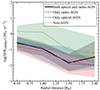 |
Fig. 5. Radial profiles of recent (100 Myr) SFRs of the different source groups, discussed in Sects. 4.1 and 4.2. The lines show the median SFRs and the shaded regions mark the 25th and 75th percentile values of the SFR distributions. SFRs for the non-AGN group are larger at every radial point than the AGN groups. |
4.2. Dependence on radio luminosity
The total mechanical energy output of a radio-AGN is correlated to L1.4 GHz (e.g. Cavagnolo et al. 2010; McNamara & Nulsen 2012). Therefore, investigating the dependence of [O III] kinematics on radio luminosity can help understand the relation between feedback and the total mechanical energy emitted. Using the spatially resolved maps we can determine if the scales on which [O III] is disturbed change with L1.4 GHz. Since the radio-AGN sample also has some optical-AGN, we handle the radio-AGN sources with and without an optical-AGN separately, as done above. We then split the sample into groups of radio luminosity at L1.4 GHz = 1023 W Hz−1. Low L1.4 GHz sources cover a luminosity range of 1021 − 1023 W Hz−1 and high L1.4 GHz sources from 1023 − 1025 W Hz−1, although most sources in the high L1.4 GHz groups are between 1023 − 1024 W Hz−1. In the group of radio+optical AGN, this gives 20 low L1.4 GHz sources and 12 high L1.4 GHz sources. In the group of radio-AGN, this gives 142 low L1.4 GHz sources and 42 high L1.4 GHz sources (summarised in Table 3).
The radial profiles of these four groups are shown in Fig. 6. We find that the median values of ![Mathematical equation: $ W^{[{\mathrm{O}{\small { {\text{ III}}}}}]}_{80} $](/articles/aa/full_html/2025/06/aa53307-24/aa53307-24-eq11.gif) and QW80 are largest for radio+optical AGN with high L1.4 GHz, within r = 0.25 Reff4. However, this difference is only marginally significant when compared to radio+optical AGN with low L1.4 GHz. Similarly, radio-AGN with high L1.4 GHz show larger
and QW80 are largest for radio+optical AGN with high L1.4 GHz, within r = 0.25 Reff4. However, this difference is only marginally significant when compared to radio+optical AGN with low L1.4 GHz. Similarly, radio-AGN with high L1.4 GHz show larger ![Mathematical equation: $ W^{[{\mathrm{O}{\small { {\text{ III}}}}}]}_{80} $](/articles/aa/full_html/2025/06/aa53307-24/aa53307-24-eq12.gif) and QW80 up to r = 0.5 Reff, but it is only marginally significant till r = 0.25 Reff. Judging by the p values of the distributions beyond r = 0.5 Reff, we find that distributions for all groups agree with each other. This shows that the presence of a moderately powerful radio+optical AGN disturbs the [O III] gas most, although the spatial extent at which gas is disturbed does not increase at higher L1.4 GHz.
and QW80 up to r = 0.5 Reff, but it is only marginally significant till r = 0.25 Reff. Judging by the p values of the distributions beyond r = 0.5 Reff, we find that distributions for all groups agree with each other. This shows that the presence of a moderately powerful radio+optical AGN disturbs the [O III] gas most, although the spatial extent at which gas is disturbed does not increase at higher L1.4 GHz.
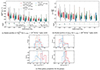 |
Fig. 6. Same radial profiles in (a) and (b) as in Fig. 4 but for high and low L1.4 GHz radio+optical AGN and radio-AGN sources. The colours in panel c represent the same sources as in the top panels. |
Looking at the QW80 radial profiles of the radio+optical AGN with low L1.4 GHz in Fig. 6b, it is interesting to note that they have a tail of high QW80 values out to large radial distances (r = 1.75 Reff). However, this tail is not visible in the radio+optical AGN with high L1.4 GHz. We described this tail in the previous section. Given that its most prominent in low L1.4 GHz radio+optical AGN, a likely explanation for this could be that the radio emission observed in these sources is due to shocks driven by the radiation from the optical-AGN; therefore, it would be an effect coming from the disturbed ionised gas and not the cause. This shock interpretation is discussed more in Sect. 5.
5. Discussion
In this paper, we study the impact of low-to-moderate-luminosity radio- and optical-AGN on the [O III] gas in the Local Universe up to z ≈ 0.15. We selected a sample of 806 nearby radio-AGN from the MaNGA catalogue, using a combination of LoTSS and FIRST surveys, out of which 378 have an [O III] detection. We then controlled for host galaxy properties and finally used a sample of 32 radio+optical AGN, 184 radio-AGN, 22 optical AGN, and 28 non AGN sources for our analysis. Constructing such groups allowed us to systematically study the feedback from radio and optical AGN selected from the same survey. Using spatially resolved maps of [O III] spectra, we constructed radial profiles of ![Mathematical equation: $ W^{[{\mathrm{O}{\small { {\text{ III}}}}}]}_{80} $](/articles/aa/full_html/2025/06/aa53307-24/aa53307-24-eq13.gif) and QW80, to study the impact on the warm ionised gas. Our sample covers a radio luminosity range of L1.4 GHz ≈ 1021 − 1024 W Hz−1, including systems that are traditionally called radio-loud and radio-quiet AGN.
and QW80, to study the impact on the warm ionised gas. Our sample covers a radio luminosity range of L1.4 GHz ≈ 1021 − 1024 W Hz−1, including systems that are traditionally called radio-loud and radio-quiet AGN.
5.1. Impact of radio-AGN on [O III]
Comparing the ![Mathematical equation: $ W^{[{\mathrm{O}{\small { {\text{ III}}}}}]}_{80} $](/articles/aa/full_html/2025/06/aa53307-24/aa53307-24-eq14.gif) and QW80 radial profiles of different AGN groups from our sample allows us to determine the presence of disturbed [O III] and its relation to the radio- and optical-AGN. Comparing the QW80 profiles of all sources in Fig. 4, we find a statistically significant difference at r = 0.25 Reff, between sources that have radio+optical AGN and sources that have only either a radio- or an optical-AGN. We also find that when radio+optical AGN are present, more than half the sources have QW80 > 1 at r = 0.25 Reff. This shows that [O III] is more disturbed than when radio+optical AGN are present, compared to when only either one is present. The radial distance of r = 0.25 Reff, corresponds to a physical radial distance range of ∼0.5 − 5.9 kpc for our sample and 1.9 kpc at the median redshift. We propose that the warm ionised gas in nearby AGN host galaxies is disturbed on compact scales. Similar results for the compact nature of disturbed ionised gas have been found before (for example Tadhunter et al. 2018; Holden & Tadhunter 2025).
and QW80 radial profiles of different AGN groups from our sample allows us to determine the presence of disturbed [O III] and its relation to the radio- and optical-AGN. Comparing the QW80 profiles of all sources in Fig. 4, we find a statistically significant difference at r = 0.25 Reff, between sources that have radio+optical AGN and sources that have only either a radio- or an optical-AGN. We also find that when radio+optical AGN are present, more than half the sources have QW80 > 1 at r = 0.25 Reff. This shows that [O III] is more disturbed than when radio+optical AGN are present, compared to when only either one is present. The radial distance of r = 0.25 Reff, corresponds to a physical radial distance range of ∼0.5 − 5.9 kpc for our sample and 1.9 kpc at the median redshift. We propose that the warm ionised gas in nearby AGN host galaxies is disturbed on compact scales. Similar results for the compact nature of disturbed ionised gas have been found before (for example Tadhunter et al. 2018; Holden & Tadhunter 2025).
Beyond this point, we find that the QW80 radial profiles of all AGN groups are largely similar, except the high values that create the tails seen in the distributions of radio+optical AGN. Although similar trends can be seen in the ![Mathematical equation: $ W^{[{\mathrm{O}{\small { {\text{ III}}}}}]}_{80} $](/articles/aa/full_html/2025/06/aa53307-24/aa53307-24-eq15.gif) radial profiles of the different groups, the differences between them are suppressed when normalising them with
radial profiles of the different groups, the differences between them are suppressed when normalising them with  . This shows that the differences in the [O III] kinematics can also be attributed to locally different gravitational motions and a difference in
 ![Mathematical equation: $ W^{[{\mathrm{O}{\small { {\text{ III}}}}}]}_{80} $](/articles/aa/full_html/2025/06/aa53307-24/aa53307-24-eq17.gif) does not necessarily imply more or less disturbed [O III] kinematics. This highlights the advantage and necessity of using QW80 values for comparing different sources.
does not necessarily imply more or less disturbed [O III] kinematics. This highlights the advantage and necessity of using QW80 values for comparing different sources.
In the radio+optical AGN group, both jets and shocks can be responsible for the observed radio emission, as discussed in Sect. 2.1. In the case of jets, the presence of more disturbed [O III] in radio+optical AGN would point to a co-active role of jets and radiation, such that when both are present, the impact on warm ionised gas kinematics is the strongest. In the case of radiative wind-driven shocks, this would mean that the disturbed [O III] is essentially tracing sources with strong shocks, which cause the radio emission. Therefore, the radio-emission would not be the cause but the effect of the feedback on the host galaxy.
Differentiating between the two cases would ideally require high-resolution radio imaging and radio spectral analysis. Lacking this information for the sample, splitting the radio+optical AGN sample into high and low L1.4 GHz sources sheds some light on this. We find that the trend we discussed above, with more than half of these sources having QW80 > 1 at r = 0.25 Reff, is driven by the high luminosity sample, as can be seen in Fig. 6. These systems are more likely to have their radio emission dominated by jets, as can be seen by their positions with respect to the models in Fig. 2. Therefore, we propose that in these systems, the radio emission is dominated by jets and the signatures of disturbed ionised gas observed on small scales are likely due to jet-ISM interaction.
However, the prominent tail of large ![Mathematical equation: $ W^{[{\mathrm{O}{\small { {\text{ III}}}}}]}_{80} $](/articles/aa/full_html/2025/06/aa53307-24/aa53307-24-eq18.gif) and QW80 values in the low L1.4 GHz sources likely point towards a shock origin of radio emission in these systems (although beam smearing also contributes to this, as mentioned before). Indeed, these systems also fall on or below the (Nims et al. 2015) models shown in Fig. 2. Therefore, it is possible that at these low radio luminosities, the high [O III] line widths are a selection effect, as selecting radio-AGN essentially means searching for sources with strong shocks. Overall, this highlights the role of both sources of radio emission in understanding feedback in low-to-moderate radio-luminosity systems.
and QW80 values in the low L1.4 GHz sources likely point towards a shock origin of radio emission in these systems (although beam smearing also contributes to this, as mentioned before). Indeed, these systems also fall on or below the (Nims et al. 2015) models shown in Fig. 2. Therefore, it is possible that at these low radio luminosities, the high [O III] line widths are a selection effect, as selecting radio-AGN essentially means searching for sources with strong shocks. Overall, this highlights the role of both sources of radio emission in understanding feedback in low-to-moderate radio-luminosity systems.
Our results reinforce the positive correlation between disturbed [O III] kinematics and the presence of radio emission in AGN host galaxies, which has also been observed before with SDSS single fibre spectra that cover the central 3″ of the galaxies (e.g. Mullaney et al. 2013; Woo et al. 2016; Molyneux et al. 2019; Kukreti et al. 2023; Kukreti & Morganti 2024). Recently, using a sample of ∼5700 radio-AGN and SDSS spectra, Kukreti & Morganti (2024) found a positive correlation between the [O III] line-widths and L1.4 GHz, with more disturbed gas sources with L1.4 GHz > 1023 W Hz−1. Using a large sample of ≈24 000 type 1 and 2 AGN, Mullaney et al. (2013) also found that the width of [O III] profiles was larger for AGN with a radio detection, peaking between 1023 − 1025 W Hz−1. However, the sources in this study were not selected to be radio-AGN, and the shock origin of radio-emission could be quite significant contributor in this sample. Although the single fibre spectra used in these studies only cover the innermost region of our galaxies as mentioned above, our results are still in agreement with these studies over that region. The 0.25 Reff point up to which we detect disturbed [O III] covers the same size of central region as the SDSS single fibre studies at these redshifts. However, the spatially resolved MaNGA IFU data allows us to investigate the impact on larger scales, where we find no significant differences in the impact of various low-to-moderate-luminosity AGN groups.
5.2. The simultaneous impact of jets and radiation
Separating sources with a radio+optical AGN from those with either only a radio-AGN or only an optical-AGN allows us to perform a comparative analysis of the role of jets and radiation in low-to-moderate-luminosity AGN. This is illustrated in Fig. 6, which shows the ![Mathematical equation: $ W^{[{\mathrm{O}{\small { {\text{ III}}}}}]}_{80} $](/articles/aa/full_html/2025/06/aa53307-24/aa53307-24-eq19.gif) and QW80 radial profiles for different L1.4 GHz of radio-AGN sources, with and without an optical-AGN. When radio+optical AGN are present in a source, we find that [O III] is more likely to be disturbed on small scales (when the radio-AGN has L1.4 GHz > 1023 W Hz−1) than when it is less luminous.
and QW80 radial profiles for different L1.4 GHz of radio-AGN sources, with and without an optical-AGN. When radio+optical AGN are present in a source, we find that [O III] is more likely to be disturbed on small scales (when the radio-AGN has L1.4 GHz > 1023 W Hz−1) than when it is less luminous.
Even though optical-AGN of similar [O III] luminosities are present in both L1.4 GHz groups, the presence of more powerful jets correlates with relatively more disturbed [O III], judging by the difference in QW80 values. These jets are likely the source of radio emission in the high L1.4 GHz sources, as mentioned above. This group of radio+optical AGN has more disturbed [O III] sources at 0.25 Reff than their low L1.4 GHz counterparts and the optical-AGN group. This shows that when moderately powerful radio-AGN and optical-AGN are present in a source simultaneously, the gas is most likely to be disturbed. Therefore, jets and radiation in these systems seem to be acting in a manner where the both enhance the impact of each other on the surrounding ionised gas kinematics. When radiation pressure from the AGN is present along with the jets, the AGN is more effective in disturbing the [O III] kinematics than it would be if it only had jets (and vice versa). Comparing only points with QW80 > 1, we see that the impact is strongest for the group with radio+optical AGN and radio-AGN with high L1.4 GHz. We recall here that sources with L1.4 GHz > 1023 W Hz−1 are still moderate-luminosity sources, with typical luminosities between 1023 − 1024 W Hz−1.
Our results show that the strongest impact of jets in radio+optical AGN systems is limited to the central region of the galaxies. Comparing the radio sizes and optical host galaxy sizes sheds some more light on this trend. The ratio between the radio sizes of our sources, which we have taken from the LoTSS value-added catalogue of Hardcastle et al. (2023), and the effective radii of the host galaxies has a median value of 0.5. This means that the radio emission from the AGN is typically on much smaller scales than the host galaxy size. This explains why the impact we see on [O III] in the L1.4 GHz > 1023 W Hz−1 radio-AGN groups, is limited to the central region.
Combining this finding with the results discussed above, we propose a scenario in which jet and radiation-driven feedback are simultaneously active in moderate-luminosity radio-AGN host galaxies. The ionised gas appears to be impacted by both, as can be seen in the highly disturbed radial profiles of sources that have both types of AGN. This shows that feedback on ionised gas in AGN selected based on their having radio jets is not necessarily only driven by the jets. The presence of radiation from the AGN makes it more likely for the gas to be kinematically disturbed in radio-AGN host galaxies, compared to the case where only jets are present. Furthermore, comparing the radio-AGN groups with and without an optical-AGN suggests that gas clouds, perhaps pushed to high velocities by the jets, are driven to even higher velocities by the impact of radiation, and vice versa.
5.3. Feedback in low-to-moderate-luminosity radio-AGN
Feedback on [O III] in radio-AGN host galaxies was also studied by Albán et al. (2024), and we used the same routine to extract the radial W80 profiles for our study. In their analysis, Albán et al. (2024) found that radio-AGN exhibit larger W80 values at large Reff in comparison to broad-line and optical AGN, even when the samples are matched in host galaxy properties. We find that [O III] is most disturbed, in terms of the gas velocity and proportion of sources disturbed, in the central region when radio+optical AGN are present. The impact is relatively milder when either only radio- or optical-AGN are present. This is qualitatively in agreement with the results of Albán et al. (2024); however, the differences we find in the impact on [O III] are limited to a radial distance of 0.25 Reff. The differences in the [O III] line widths reported by Albán et al. (2024) beyond this distance could be due to the low-luminosity radio+optical AGN that we have in our sample.
It is also worth noting that these differences could be due to the differences in the selection techniques and the host galaxies of the radio-AGN selected. The radio-AGN we selected are predominantly hosted by passive early-type galaxies, whereas theirs are equally distributed among early and late-type galaxies. Since early-type galaxies are dispersion-dominated and passive in terms of star formation, their QW80 and SFR are lower than late-type galaxies. This explains the differences observed in the two samples at larger radii. Indeed, setting controls for early-type (or late-type) galaxies brings the radial profiles in agreement with each other.
Our results propose a scenario in which the impact of low-to-moderate-luminosity radio-AGN is strongest on the ionised gas in the central 0.25 Reff region of galaxies in the Local Universe. The lifetime of a radio-AGN phase of ∼10 − 100 Myr is significantly smaller than the galaxy’s lifetime of a few Gyr (see Morganti 2017 for a review). Therefore, a single phase of activity is unlikely to impact star-formation significantly over the galaxy’s lifetime. Indeed, many radio-AGN with multiple epochs of activity have been detected (e.g. Sridhar et al. 2020; Brienza et al. 2020; Kukreti et al. 2022), pushing the need to understand the cumulative impact of multiple AGN phases on the galaxy. If every phase of activity had the strongest impact on the gas in the central regions, we would expect to see less star formation in these regions compared to non-AGN host galaxies. Evidence for such inside-out quenching has been found in MaNGA galaxies, albeit in AGN selected using emission line ratios (e.g. Bluck et al. 2020; Lammers et al. 2023; Bertemes et al. 2022). AGN feedback over multiple phases of activity could have suppressed the star formation in the central regions of these galaxies. Although we are studying the warm ionised phase, which is not the fuel for star formation, our results provide evidence supporting this scenario. Further studies of feedback in restarted radio-AGN on molecular gas phases (fuel for star formation) would be required to test these scenarios. We plan to conduct such studies in the future.
6. Summary
We selected a sample of radio-AGN using LoTSS and FIRST surveys and combined them with MaNGA to obtain spatially resolved spectra for a subsample over a redshift range of z = 0.01 − 0.15. The radio-AGN were selected on the basis of their greater radio emission compared to what is otherwise expected from star formation and are low-to-moderate radio and [O III] luminosity sources. We assessed the impact of radio and optical-AGN on the [O III] kinematics in these sources, to disentangle the role of jets and radiation in driving feedback. Our main finding is that when radio+optical AGN are present, sources are significantly more likely to have disturbed [O III] up to a radial distance of 0.25 Reff, than when there is either only a radio- or optical-AGN present. This shows that when both jets and radiation are present in a system, AGN have the strongest impact on the surrounding warm ionised gas. This relation is dependent on radio luminosity and so, high radio luminosity sources are more likely to have more disturbed gas in the central region. We note that in low radio-luminosity radio+optical AGN, the observed radio emission could be due to wind-driven shocks instead of jets. However, this does not affect our results, which are mainly driven by higher radio-luminosity AGN. Finally, we find that any differences in the impact on [O III] are only visible up to a radial distance of 0.25 Reff. We find no evidence of a broader, large-scale impact of moderate-luminosity jets on the warm ionised gas in these galaxies.
Both tracks were provided by Philip Best (private communication).
Private communication.
The QW80 radial profiles of this group have very few (< 5) points beyond r = 1 Reff, therefore the distributions are not reliable and are not shown here.
Acknowledgments
We thank the anonymous referee for the feedback and suggestions, that improved the paper. D.W. acknowledges support through an Emmy Noether Grant of the German Research Foundation, a stipend by the Daimler and Benz Foundation and a Verbundforschung grant by the German Space Agency. BDO acknowledges the support from the Coordenação de Aperfeiçoamento de Pessoal de Nível Superior (CAPES-Brasil, 88887.985730/2024-00). This project makes use of the MaNGA-Pipe3D dataproducts. We thank the IA-UNAM MaNGA team for creating this catalogue, and the Conacyt Project CB-285080 for supporting them. Funding for the Sloan Digital Sky Survey IV has been provided by the Alfred P. Sloan Foundation, the U.S. Department of Energy Office of Science, and the Participating Institutions. SDSS-IV acknowledges support and resources from the Center for High-Performance Computing at the University of Utah. The SDSS website is www.sdss.org
References
- Albán, M., & Wylezalek, D. 2023, A&A, 674, A85 [NASA ADS] [CrossRef] [EDP Sciences] [Google Scholar]
- Albán, M., Wylezalek, D., Comerford, J. M., Greene, J. E., & Riffel, R. A. 2024, A&A, 691, A124 [NASA ADS] [CrossRef] [EDP Sciences] [Google Scholar]
- Ayubinia, A., Woo, J.-H., Rakshit, S., & Son, D. 2023, ApJ, 954, 27 [NASA ADS] [CrossRef] [Google Scholar]
- Becker, R. H., White, R. L., Helfand, D. J., et al. 1995, ApJ, 450, 559 [Google Scholar]
- Bertemes, C., Wylezalek, D., Albán, M., et al. 2022, MNRAS, 518, 5500 [Google Scholar]
- Best, P. N., & Heckman, T. M. 2012, MNRAS, 421, 1569 [NASA ADS] [CrossRef] [Google Scholar]
- Best, P. N., Kauffmann, G., & Heckman, T. M. 2005, MNRAS, 362, 9 [NASA ADS] [CrossRef] [Google Scholar]
- Bluck, A. F., Maiolino, R., Piotrowska, J. M., et al. 2020, MNRAS, 499, 230 [NASA ADS] [CrossRef] [Google Scholar]
- Boroson, T. A. 2002, ApJ, 585, 647 [Google Scholar]
- Brienza, M., Morganti, R., Harwood, J., et al. 2020, A&A, 638, A29 [EDP Sciences] [Google Scholar]
- Brinchmann, J., Charlot, S., Heckman, T. M., et al. 2004, ArXiv e-prints [arXiv:astro-ph/0406220] [Google Scholar]
- Bundy, K., Bershady, M. A., Law, D. R., et al. 2015, ApJ, 798, 7 [Google Scholar]
- Cavagnolo, K. W., McNamara, B. R., Nulsen, P. E. J., et al. 2010, ApJ, 720, 1066 [Google Scholar]
- Cid Fernandes, R., Stasińska, G., Schlickmann, M. S., et al. 2010, MNRAS, 403, 1036 [Google Scholar]
- Cid Fernandes, R., Stasinska, G., Mateus, A., & Asari, N. V. 2011, MNRAS, 413, 1687 [NASA ADS] [CrossRef] [Google Scholar]
- Comerford, J. M., Nevin, R., Negus, J., et al. 2024, ApJ, 963, 53 [NASA ADS] [CrossRef] [Google Scholar]
- Condon, J. J., Cotton, W. D., Greisen, E. W., et al. 1998, AJ, 115, 1693 [Google Scholar]
- Cresci, G., Tozzi, G., Perna, M., et al. 2023, A&A, 672, A128 [NASA ADS] [CrossRef] [EDP Sciences] [Google Scholar]
- Cutri, R. M., Wright, E. L., Conrow, T., et al. 2021, VizieR Online Data Catalog: II/328 [Google Scholar]
- Deconto-Machado, A., Riffel, R. A., Ilha, G. S., et al. 2022, A&A, 659, 131 [Google Scholar]
- Di Matteo, T., Springel, V., & Ilernquist, L. 2005, Nature, 433, 604 [NASA ADS] [CrossRef] [Google Scholar]
- Domínguez Sánchez, H., Margalef, B., Bernardi, M., & Huertas-Company, M. 2022, MNRAS, 509, 4024 [Google Scholar]
- Fabian, A. C. 2012, ARA&A, 50, 455 [Google Scholar]
- Faucher-Giguère, C. A., & Quataert, E. 2012, MNRAS, 425, 605 [NASA ADS] [CrossRef] [Google Scholar]
- Fischer, J. L., Domínguez Sánchez, H., & Bernardi, M. 2019, MNRAS, 483, 2057 [NASA ADS] [CrossRef] [Google Scholar]
- Fu, Y., Cappellari, M., Mao, S., et al. 2023, MNRAS, 524, 5827 [CrossRef] [Google Scholar]
- Galvin, T. J., Huynh, M. T., Norris, R. P., et al. 2020, MNRAS, 497, 2730 [NASA ADS] [CrossRef] [Google Scholar]
- Gatto, L., Storchi-Bergmann, T., Riffel, R. A., et al. 2024, MNRAS, 530, 3059 [NASA ADS] [CrossRef] [Google Scholar]
- Girdhar, A., Harrison, C. M., Mainieri, V., et al. 2022, MNRAS, 512, 1608 [NASA ADS] [CrossRef] [Google Scholar]
- Gürkan, G., Hardcastle, M. J., Smith, D. J., et al. 2018, MNRAS, 475, 3010 [CrossRef] [Google Scholar]
- Hardcastle, M. J., Horton, M. A., Williams, W. L., et al. 2023, A&A, 678, A151 [NASA ADS] [CrossRef] [EDP Sciences] [Google Scholar]
- Harrison, C. M., & Ramos Almeida, C. 2024, Galaxies, 12, 17 [NASA ADS] [CrossRef] [Google Scholar]
- Heckman, T. M., Kauffmann, G., Brinchmann, J., et al. 2004, ApJ, 613, 109 [Google Scholar]
- Heckman, T. M., Alexandroff, R. M., Borthakur, S., Overzier, R., & Leitherer, C. 2015, ApJ, 809, 147 [Google Scholar]
- Herpich, F., Mateus, A., Stasińska, G., Fernandes, R. C., & Asari, N. V. 2016, MNRAS, 462, 1826 [NASA ADS] [CrossRef] [Google Scholar]
- Holden, L. R., & Tadhunter, C. N. 2025, MNRAS, 536, 1857 [Google Scholar]
- Jarvis, M. E., Harrison, C. M., Thomson, A. P., et al. 2019, MNRAS, 485, 2710 [Google Scholar]
- Jarvis, M. E., Harrison, C. M., Mainieri, V., et al. 2021, MNRAS, 503, 1780 [NASA ADS] [CrossRef] [Google Scholar]
- Kang, D., & Woo, J.-H. 2018, ApJ, 864, 124 [NASA ADS] [CrossRef] [Google Scholar]
- Kauffmann, G., Heckman, T. M., Tremonti, C., et al. 2003, MNRAS, 346, 1055 [Google Scholar]
- Kauffmann, G., Heckman, T. M., & Best, P. N. 2008, MNRAS, 384, 953 [Google Scholar]
- Kewley, L. J., Groves, B., Kauffmann, G., & Heckman, T. 2006, MNRAS, 372, 961 [Google Scholar]
- Kim, C., Woo, J.-H., Luo, R., et al. 2023, ApJ, 958, 145 [NASA ADS] [CrossRef] [Google Scholar]
- King, A., & Pounds, K. 2015, A&AR, 53, 115 [Google Scholar]
- Kukreti, P., & Morganti, R. 2024, A&A, 690, A140 [NASA ADS] [CrossRef] [EDP Sciences] [Google Scholar]
- Kukreti, P., Morganti, R., Shimwell, T. W., et al. 2022, A&A, 658, A6 [NASA ADS] [CrossRef] [EDP Sciences] [Google Scholar]
- Kukreti, P., Morganti, R., Tadhunter, C., & Santoro, F. 2023, A&A, 674, A198 [NASA ADS] [CrossRef] [EDP Sciences] [Google Scholar]
- Lacerda, E. A., Sánchez, S. F., Mejía-Narváez, A., et al. 2022, New Astron., 97, 101895 [NASA ADS] [CrossRef] [Google Scholar]
- Lammers, C., Iyer, K. G., Ibarra-Medel, H., et al. 2023, ApJ, 953, 26 [NASA ADS] [CrossRef] [Google Scholar]
- Law, D. R., Cherinka, B., Yan, R., et al. 2016, AJ, 152, 83 [Google Scholar]
- Law, D. R., Westfall, K. B., Bershady, M. A., et al. 2021, AJ, 161, 52 [NASA ADS] [CrossRef] [Google Scholar]
- McNamara, B. R., & Nulsen, P. E. 2007, ARA&A, 45, 117 [NASA ADS] [CrossRef] [Google Scholar]
- McNamara, B. R., & Nulsen, P. E. 2012, New J. Phys., 14, 055023 [NASA ADS] [CrossRef] [Google Scholar]
- Mingo, B., Watson, M. G., Rosen, S. R., et al. 2016, MNRAS, 462, 2631 [NASA ADS] [CrossRef] [Google Scholar]
- Molyneux, S. J., Harrison, C. M., & Jarvis, M. E. 2019, A&A, 631, A132 [NASA ADS] [CrossRef] [EDP Sciences] [Google Scholar]
- Morganti, R. 2017, Nat. Astron., 1, 596 [Google Scholar]
- Morganti, R. 2021, Proc. Int. Astron. Union, 356, 229 [Google Scholar]
- Mulcahey, C. R., Leslie, S. K., Jackson, T. M., et al. 2022, A&A, 665, A144 [NASA ADS] [CrossRef] [EDP Sciences] [Google Scholar]
- Mullaney, J. R., Alexander, D. M., Fine, S., et al. 2013, MNRAS, 433, 622 [Google Scholar]
- Murthy, S., Morganti, R., Oosterloo, T., et al. 2019, A&A, 629, A58 [NASA ADS] [CrossRef] [EDP Sciences] [Google Scholar]
- Nelson, C. H., & Whittle, M. 1996, ApJ, 465, 96 [NASA ADS] [CrossRef] [Google Scholar]
- Nesvadba, N. P. H., Wagner, A. Y., Mukherjee, D., et al. 2021, A&A, 654, 8 [Google Scholar]
- Nims, J., Quataert, E., & Faucher-Giguére, C. A. 2015, MNRAS, 447, 3612 [NASA ADS] [CrossRef] [Google Scholar]
- Riffel, R. A., Riffel, R., Bianchin, M., et al. 2023a, MNRAS, 521, 3260 [NASA ADS] [CrossRef] [Google Scholar]
- Riffel, R., Mallmann, N. D., Rembold, S. B., et al. 2023b, MNRAS, 524, 5640 [NASA ADS] [CrossRef] [Google Scholar]
- Ruffa, I., Prandoni, I., Davis, T. A., et al. 2022, MNRAS, 510, 4485 [NASA ADS] [CrossRef] [Google Scholar]
- Sabater, J., Best, P. N., Hardcastle, M. J., et al. 2019, A&A, 622, 17 [Google Scholar]
- Sadler, E. M., Jackson, C. A., Cannon, R. D., et al. 2002, MNRAS, 329, 227 [Google Scholar]
- Sánchez, S. F., Barrera-Ballesteros, J. K., Lacerda, E., et al. 2022, ApJS, 262, 36 [CrossRef] [Google Scholar]
- Santoro, F., Tadhunter, C., Baron, D., Morganti, R., & Holt, J. 2020, A&A, 644, A54 [NASA ADS] [CrossRef] [EDP Sciences] [Google Scholar]
- Sexton, R. O., Matzko, W., Darden, N., Canalizo, G., & Gorjian, V. 2020, MNRAS, 500, 2871 [NASA ADS] [CrossRef] [Google Scholar]
- Shimwell, T. W., Röttgering, H. J., Best, P. N., et al. 2017, A&A, 598, A104 [NASA ADS] [CrossRef] [EDP Sciences] [Google Scholar]
- Shimwell, T. W., Hardcastle, M. J., Tasse, C., et al. 2022, A&A, 659, A1 [NASA ADS] [CrossRef] [EDP Sciences] [Google Scholar]
- Silk, J., & Rees, M. J. 1998, A&A, 331, L1 [NASA ADS] [Google Scholar]
- Speranza, G., Balmaverde, B., Capetti, A., et al. 2021, A&A, 653, A150 [NASA ADS] [CrossRef] [EDP Sciences] [Google Scholar]
- Sridhar, S. S., Morganti, R., Nyland, K., et al. 2020, A&A, 634, A108 [NASA ADS] [CrossRef] [EDP Sciences] [Google Scholar]
- Stasińska, G., Vale Asari, N., Wójtowicz, A., & Kozieł-Wierzbowska, D. 2025, A&A, 693, A135 [NASA ADS] [CrossRef] [EDP Sciences] [Google Scholar]
- Sun, A.-L., Greene, J. E., & Zakamska, N. L. 2017, ApJ, 835, 222 [Google Scholar]
- Suresh, A., & Blanton, M. R. 2024, ApJ, 977, 194 [Google Scholar]
- Tadhunter, C., Rodríguez Zaurín, J., Rose, M., et al. 2018, MNRAS, 478, 1558 [NASA ADS] [CrossRef] [Google Scholar]
- Taylor, M. 2005, ASP Conf. Ser., 347, 29 [NASA ADS] [Google Scholar]
- Ulivi, L., Venturi, G., Cresci, G., et al. 2024, A&A, 685, 122 [Google Scholar]
- Venturi, G., Cresci, G., Marconi, A., et al. 2021, A&A, 648, A17 [NASA ADS] [CrossRef] [EDP Sciences] [Google Scholar]
- Westfall, K. B., Cappellari, M., Bershady, M. A., et al. 2019, AJ, 158, 231 [Google Scholar]
- Woo, J.-H., Bae, H.-J., Son, D., & Karouzos, M. 2016, ApJ, 817, 108 [Google Scholar]
- Woo, J.-H., Son, D., & Bae, H.-J. 2017, ApJ, 839, 120 [Google Scholar]
- Wylezalek, D., Flores, A. M., Zakamska, N. L., Greene, J. E., & Riffel, R. A. 2020, MNRAS, 492, 4680 [NASA ADS] [CrossRef] [Google Scholar]
- Yan, L., Donoso, E., Tsai, C. W., et al. 2013, AJ, 145, 55 [NASA ADS] [CrossRef] [Google Scholar]
- Zakamska, N. L., & Greene, J. E. 2014, MNRAS, 442, 784 [Google Scholar]
- Zakamska, N. L., Lampayan, K., Petric, A., et al. 2016, MNRAS, 455, 4191 [Google Scholar]
- Zubovas, K., & King, A. 2012, ApJ, 745, L34 [Google Scholar]
Appendix A: Selecting radio-AGN from FIRST
Diagnostic combinations for FIRST sources.
Classification of FIRST cross-matched sources.
All Tables
All Figures
|
Fig. 1. Diagnostic plots for selecting radio-AGN using LoTSS data. Red points mark the sources classified as radio-AGN after combining all four diagnostics, and grey points show the star-forming/radio-quiet AGN: (a) Dn(4000) vs L1.4 GHz/M⋆ plot. The solid and dashed curves mark the radio-AGN, intermediate and SF/RQAGN division from Best & Heckman (2012) and Sabater et al. (2019); (b) LHα versus L1.4 GHz plot, with the separation lines from Sabater et al. (2019); (c) BPT diagram where the solid curve shows the semi-empirical relation from Kauffmann et al. (2003), and the dashed curve shows the maximum starburst curve from Kewley et al. (2006); (d) WISE colour-colour plot for sources with the division line from Sabater et al. (2019). |
| In the text | |
|
Fig. 2. 1.4 GHz and [O III] luminosities of the sources with an [O III] detection. Sources with radio+optical AGN, radio-AGN, and optical-AGN are shown. For optical-AGN without a radio detection, the arrows show the upper limits on L1.4 GHz. The shaded regions show the expected radio luminosity from the shocks scenario using the Nims et al. (2015) model, where the lower and upper edges show the limits for 5% and 25% coupling efficiency between AGN luminosity and wind kinetic luminosity, respectively. Different regions show the [O III] to bolometric luminosity conversion factors from Heckman et al. (2004) and Stasińska et al. (2025). The horizontal dotted lines show the luminosity divisions used in Sect. 4. To highlight the low-to-moderate luminosity nature of the sources in our study, we also show the parameter space occupied by the radio-AGN sample from Kukreti & Morganti (2024) in black contours, which examines the relation between radio properties and feedback on [O III] out to z = 0.8. |
| In the text | |
|
Fig. 3. Maps of a radio-AGN from the sample (plateifu = 8714−3704). The top left image shows the SDSS optical colour image of the host galaxy, with the MaNGA FoV marked with magenta. The other panels show the stellar and [O III] emission line properties. Only spaxels with a [O III] detection of S/N > 5 are shown and used throughout the paper for analysis. The green contours show the radio emission from FIRST at 1.4 GHz in the bottom left panel. The elliptical annuli regions used for constructing radial profiles are shown in the bottom middle panel. The same plot for a non-AGN source is shown in Fig. A.2 to illustrate the differences in their gas kinematics. |
| In the text | |
|
Fig. 4. Comparison of the four groups with: an optical and radio-AGN, radio-AGN, optical-AGN, and non-AGN. Radial profiles of |
| In the text | |
|
Fig. 5. Radial profiles of recent (100 Myr) SFRs of the different source groups, discussed in Sects. 4.1 and 4.2. The lines show the median SFRs and the shaded regions mark the 25th and 75th percentile values of the SFR distributions. SFRs for the non-AGN group are larger at every radial point than the AGN groups. |
| In the text | |
|
Fig. 6. Same radial profiles in (a) and (b) as in Fig. 4 but for high and low L1.4 GHz radio+optical AGN and radio-AGN sources. The colours in panel c represent the same sources as in the top panels. |
| In the text | |
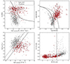 |
Fig. A.1. Same as Fig. 1, but selecting radio-AGN using FIRST data. |
| In the text | |
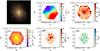 |
Fig. A.2. Same as Fig. 3, but for a non-AGN galaxy (plateifu = 12068-6104). |
| In the text | |
Current usage metrics show cumulative count of Article Views (full-text article views including HTML views, PDF and ePub downloads, according to the available data) and Abstracts Views on Vision4Press platform.
Data correspond to usage on the plateform after 2015. The current usage metrics is available 48-96 hours after online publication and is updated daily on week days.
Initial download of the metrics may take a while.