| Issue |
A&A
Volume 692, December 2024
|
|
|---|---|---|
| Article Number | A254 | |
| Number of page(s) | 21 | |
| Section | Planets, planetary systems, and small bodies | |
| DOI | https://doi.org/10.1051/0004-6361/202451068 | |
| Published online | 17 December 2024 | |
Hints of a close outer companion to the ultra-hot Jupiter TOI-2109 b★
1
Institute of Planetary Research, German Aerospace Center (DLR),
Rutherfordstrasse 2,
12489
Berlin,
Germany
2
Instituto de Astrofisica e Ciencias do Espaco, Universidade do Porto,
CAUP, Rua das Estrelas,
4150-762
Porto,
Portugal
3
Departamento de Fisica e Astronomia, Faculdade de Ciencias, Universidade do Porto,
Rua do Campo Alegre,
4169-007
Porto,
Portugal
4
INAF, Osservatorio Astrofisico di Catania,
Via S. Sofia 78,
95123
Catania,
Italy
5
Lund Observatory, Division of Astrophysics, Department of Physics, Lund University,
Box 118,
22100
Lund,
Sweden
6
Department of Astronomy, Stockholm University, AlbaNova University Center,
10691
Stockholm,
Sweden
7
Centre for Exoplanet Science, SUPA School of Physics and Astronomy, University of St Andrews,
North Haugh,
St Andrews
KY16 9SS,
UK
8
Observatoire astronomique de l’Université de Genève,
Chemin Pegasi 51,
1290
Versoix,
Switzerland
9
Department of Physics, University of Warwick,
Gibbet Hill Road,
Coventry
CV4 7AL,
UK
10
INAF, Osservatorio Astronomico di Padova,
Vicolo dell’Osservatorio 5,
35122
Padova,
Italy
11
CFisUC, Department of Physics, University of Coimbra,
3004-516
Coimbra,
Portugal
12
Dipartimento di Fisica e Astronomia, Università degli Studi di Padova,
Vicolo dell’Osservatorio 3,
35122
Padova,
Italy
13
Center for Space and Habitability, University of Bern,
Gesellschaftsstrasse 6,
3012
Bern,
Switzerland
14
Weltraumforschung und Planetologie, Physikalisches Institut, University of Bern,
Gesellschaftsstrasse 6,
3012
Bern,
Switzerland
15
Instituto de Astrofísica de Canarias,
Vía Láctea s/n,
38200
La Laguna,
Tenerife,
Spain
16
Departamento de Astrofísica, Universidad de La Laguna,
Astrofísico Francisco Sanchez s/n,
38206
La Laguna,
Tenerife,
Spain
17
European Space Agency (ESA), ESTEC,
Keplerlaan 1,
2201 AZ
Noordwijk,
The Netherlands
18
Admatis,
5. Kandó Kálmán Street,
3534
Miskolc,
Hungary
19
Depto. de Astrofísica, Centro de Astrobiología (CSIC-INTA),
ESAC campus,
28692
Villanueva de la Cañada (Madrid),
Spain
20
Space Research Institute, Austrian Academy of Sciences,
Schmiedlstrasse 6,
8042
Graz,
Austria
21
Physikalisches Institut, University of Bern,
Gesellschaftsstrasse 6,
3012
Bern,
Switzerland
22
INAF, Osservatorio Astrofisico di Torino,
Via Osservatorio, 20,
10025
Pino Torinese To,
Italy
23
Centre for Mathematical Sciences, Lund University,
Box 118,
221 00
Lund,
Sweden
24
Aix Marseille Univ, CNRS, CNES, LAM,
38 rue Frédéric Joliot-Curie,
13388
Marseille,
France
25
Astrobiology Research Unit, Université de Liège,
Allée du 6 Août 19C,
4000
Liège,
Belgium
26
Space sciences, Technologies and Astrophysics Research (STAR) Institute, Université de Liège,
Allée du 6 Août 19C,
4000
Liège,
Belgium
27
Institute of Astronomy, KU Leuven,
Celestijnenlaan 200D,
3001
Leuven,
Belgium
28
ELTE Gothard Astrophysical Observatory,
9700
Szombathely,
Szent Imre h. u. 112,
Hungary
29
SRON Netherlands Institute for Space Research,
Niels Bohrweg 4,
2333 CA
Leiden,
The Netherlands
30
Centre Vie dans l’Univers, Faculté des sciences, Université de Genève,
Quai Ernest-Ansermet 30,
1211
Genève 4,
Switzerland
31
Leiden Observatory, University of Leiden,
PO Box 9513,
2300 RA
Leiden,
The Netherlands
32
Department of Space, Earth and Environment, Chalmers University of Technology,
Onsala Space Observatory,
439 92
Onsala,
Sweden
33
Dipartimento di Fisica, Università degli Studi di Torino,
via Pietro Giuria 1,
10125
Torino,
Italy
34
National and Kapodistrian University of Athens, Department of Physics,
University Campus, Zografos
157 84,
Athens,
Greece
35
Department of Astrophysics, University of Vienna,
Türkenschanzstrasse 17,
1180
Vienna,
Austria
36
European Space Agency (ESA), European Space Research and Technology Centre (ESTEC),
Keplerlaan 1,
2201 AZ
Noordwijk,
The Netherlands
37
Institute for Theoretical Physics and Computational Physics, Graz University of Technology,
Petersgasse 16,
8010
Graz,
Austria
38
Konkoly Observatory, Research Centre for Astronomy and Earth Sciences,
1121
Budapest,
Konkoly Thege Miklós út 15–17,
Hungary
39
ELTE Eötvös Loránd University, Institute of Physics,
Pázmány Péter sétány 1/A,
1117
Budapest,
Hungary
40
IMCCE, UMR8028 CNRS, Observatoire de Paris, PSL Univ., Sorbonne Univ.,
77 av. Denfert-Rochereau,
75014
Paris,
France
41
Institut d’astrophysique de Paris, UMR7095 CNRS, Université Pierre & Marie Curie,
98bis blvd. Arago,
75014
Paris,
France
42
Astrophysics Group, Lennard Jones Building, Keele University,
Staffordshire,
ST5 5BG,
UK
43
European Space Agency, ESA – European Space Astronomy Centre,
Camino Bajo del Castillo s/n,
28692
Villanueva de la Cañada, Madrid,
Spain
44
Institute of Optical Sensor Systems, German Aerospace Center (DLR),
Rutherfordstrasse 2,
12489
Berlin,
Germany
45
Dipartimento di Fisica e Astronomia “Galileo Galilei”, Università degli Studi di Padova,
Vicolo dell’Osservatorio 3,
35122
Padova,
Italy
46
ETH Zurich, Department of Physics,
Wolfgang-Pauli-Strasse 2,
8093
Zurich,
Switzerland
47
Cavendish Laboratory,
JJ Thomson Avenue,
Cambridge
CB3 0HE,
UK
48
Institut fuer Geologische Wissenschaften, Freie Universitaet Berlin,
Maltheserstrasse 74-100,
12249
Berlin,
Germany
49
Institut de Ciencies de l’Espai (ICE, CSIC),
Campus UAB, Can Magrans s/n,
08193
Bellaterra,
Spain
50
Institut d’Estudis Espacials de Catalunya (IEEC),
08860
Castelldefels (Barcelona),
Spain
51
HUN-REN-ELTE Exoplanet Research Group,
Szent Imre h. u. 112.,
Szombathely
9700,
Hungary
52
Institute of Astronomy, University of Cambridge,
Madingley Road,
Cambridge
CB3 0HA,
UK
53
Centre for Exoplanets and Habitability, University of Warwick,
Gibbet Hill Road,
Coventry
CV4 7AL,
UK
54
Department of Physics, University of Warwick,
Gibbet Hill Road,
Coventry
CV4 7AL,
UK
★★ Corresponding author; This email address is being protected from spambots. You need JavaScript enabled to view it.
Received:
11
June
2024
Accepted:
8
November
2024
Abstract
Context. Hot Jupiters (HJs) with close-by planetary companions are rare, with only a handful of them having been discovered so far. This could be due to their suggested dynamical histories, which lead to the possible ejection of other planets. TOI-2109 b is special in this regard because it is the HJ with the closest relative separation from its host star, being separated by less than 2.3 stellar radii. Unexpectedly, transit timing measurements from recently obtained CHEOPS observations show low-amplitude transit-timing variations (TTVs).
Aims. We aim to search for signs of orbital decay and to characterise the apparent TTVs in an attempt to gain information about a possible companion.
Methods. We fitted the newly obtained CHEOPS light curves using TLCM and extracted the resulting mid-transit timings. Successively, we used these measurements in combination with TESS and archival photometric data and radial velocity (RV) data to estimate the rate of tidal orbital decay of TOI-2109 b, and also to characterise the TTVs using the N-body code TRADES and the photo-dynamical approach of PyTTV.
Results. We find tentative evidence at 3σ for orbital decay in the TOI-2109 system when we correct the mid-transit timings using the best-fitting sinusoidal model of the TTVs. We do not detect additional transits in the available photometric data, but find evidence supporting the authenticity of the apparent TTVs, indicating a close-by, outer companion with Pc > 1.125 d. Due to the fast rotation of the star, the new planetary candidate cannot be detected in the available RV measurements, and its parameters can only be loosely constrained by our joint TTV and RV modelling.
Conclusions. TOI-2109 could join a small group of rare HJ systems that host close-by planetary companions, only one of which (WASP-47 b) has an outer companion. More high-precision photometric measurements are necessary to confirm the existence of this planetary companion.
Key words: methods: data analysis / techniques: photometric / planets and satellites: dynamical evolution and stability / planets and satellites: gaseous planets / planet-star interactions
This study uses CHEOPS data obtained as part of the Guaranteed Time Observation (GTO) programmes CH_PR100012 and CH_PR140063.
© The Authors 2024
 Open Access article, published by EDP Sciences, under the terms of the Creative Commons Attribution License (https://creativecommons.org/licenses/by/4.0), which permits unrestricted use, distribution, and reproduction in any medium, provided the original work is properly cited.
This article is published in open access under the Subscribe to Open model. This email address is being protected from spambots. You need JavaScript enabled to view it. to support open access publication.
1 Introduction
There are more than 5001 hot Jupiter (HJ) systems known, only a few of which are known to host close-by planetary companions.
These are WASP-47 (Hellier et al. 2012; Becker et al. 2015; Neveu-VanMalle et al. 2016; Nascimbeni et al. 2023), Kepler-730 (Thompson et al. 2018; Zhu et al. 2018; Cañas et al. 2019), TOI-1130 (Huang et al. 2020; Korth et al. 2023), TOI-1408 (Galazutdinov et al. 2023; Korth et al. 2024), WASP-132 (Hellier et al. 2017; Hord et al. 2022), and WASP-84 (Anderson et al. 2014; Maciejewski et al. 2023). The HJs in these systems all host only inner companions in the Earth- to Neptune-regime, except for WASP-47, which also contains a close outer sub-Neptune companion to the HJ, and a long-period giant planet. An overview of these systems is given in Fig. 1. Other systems worth mentioning are TOI-2000 (Sha et al. 2023), which contains a hot Saturn with an inner companion; TOI-5398 (Mantovan et al. 2024), which hosts a warm Saturn with an inner sub-Neptune, and WASP-148 (Hébrard et al. 2020), which consists of a hot Saturn and a non-transiting misaligned outer Saturn near a 4:1 mean-motion resonance (MMR). Furthermore, based on their analysis of the full Kepler dataset, Wu et al. (2023) find that at least 12% ± 6% of HJs should have close-by companions, indicating that there should be more of these hitherto rare systems within the sample of known HJ systems.
Theories for the origins of HJs include in situ formation, disc migration, and high-eccentricity tidal migration (for a review see e.g. Dawson & Johnson 2018). As found by Rice et al. (2022), the distributions of obliquities and eccentricities that have been observed are consistent with high-eccentricity migration and tidal damping and do not strictly require in situ formation or disc migration. Due to strong tidal interactions with their host star, misalignments and eccentricities can be damped relatively quickly, effectively erasing the imprints of formation and migration. However, this only applies to HJs that orbit cool stars, as tidal interactions are less efficient for hot host stars, as observed by Albrecht et al. (2021). A recent review of stellar obliquities is given by Albrecht et al. (2022). Violent migration scenarios, like planet–planet scattering, make it hard to explain close planetary companions to HJs. A study on in situ formation using N-body simulations that focussed on HJs with companion super-Earths found that they can produce such systems, obtaining similar occurrence rates for HJs with inner companions; however, according to these simulations, there should be fewer HJs detected as single transiting planets. A fraction of their simulations also led to two close-in gas giants (Poon et al. 2021).
Close-by planetary companions, especially when in resonance, can induce strong transit timing variations (TTVs) on one another; see for example Nascimbeni et al. (2023) for a dynamical modelling of the WASP-47 system, which makes use of high-precision CHEOPS (CHaracterising ExOPlanet Satellite) photometry. A few other prominent examples of the effect of TTVs are the Kepler-9 system (Holman et al. 2010), Kepler-80 (MacDonald et al. 2016), TRAPPIST-1 (Gillon et al. 2017; Grimm et al. 2018), and TOI-178 (Leleu et al. 2021). Examining TTVs has the potential to deliver more information about the observed system, and can be used to constrain planetary masses and the orbital periods of non-transiting companions forexample (Lithwick et al. 2012; Wu & Lithwick 2013; Hadden & Lithwick 2014, 2017).
Tidal orbital decay is caused by gravitational interactions of a planet with its host star. These interactions raise a bulge on the surface of the star, which can lead to the transfer of angular momentum between the two bodies. Orbital decay only happens if the star is rotating more slowly than the planet is orbiting around the star in the case of spin-orbit alignment because the tidal bulge will be dragged behind the moving sub-planetary point on the stellar surface. Consequently, the planetary orbit shrinks, while the star spins up (Counselman 1973; Rasio et al. 1996). There is always an offset between the position of the stellar bulge and the sub-planetary point due to the viscosity of the plasma, except if the orbital period of the planet and the rotation of the star are synchronised (see e.g. Hut 1981). Even outward migration of the planet is possible, if the star is rotating faster than the planet is orbiting. In the case of tidal orbital decay, a measure of the efficiency of the dissipation of orbital kinetic energy due to friction within the star is given by the modified stellar tidal quality factor Q′★ (Goldreich & Soter 1966). Theory suggests values ranging from 105 to 109 for stars, with smaller values indicating a higher dissipation efficiency (see e.g. Meibom & Mathieu 2005; Jackson et al. 2008; Ogilvie & Lin 2007; Penev & Sasselov 2011; Husnoo et al. 2012; Penev et al. 2012; Ogilvie 2014; Collier Cameron & Jardine 2018). Penev et al. (2018) treated Q′★ as being dependent on the tidal forcing period rather than being a constant for different stellar types, and found Q′★ in the range from 105 to 107 for orbital periods of between 0.5 days and 2 days. Measurements of Q′★ from WASP-12b and Kepler-1658 b give values of Q′★ = 1.8 × 10⁵ (Yee et al. 2020) and Q′★ = 2.5 × 10⁴ (Vissapragada et al. 2022), respectively, where the host star of the latter is a subgiant. Additionally, several lower limits for Q′★ were established in systems where tidal orbital decay could not yet be confirmed (see e.g. Maciejewski et al. 2020; Patra et al. 2020; Barros et al. 2022; Grunblatt et al. 2022; Ivshina & Winn 2022; Rosário et al. 2022; Harre et al. 2023; Wang et al. 2024).
TOI-2109 is a fast-rotating (v sin i = (81.2 ± 1.6)km s−1) F-type star with a mass of  and a radius of
  (Wong et al. 2021). It hosts an ultra-hot Jupiter, TOI-2109b, in a tight P = 0.672 d orbit, making it the HJ with the shortest orbital period known to orbit a Sun-like star, with a separation of less than 2.3 stellar radii from the centre of its host star (Wong et al. 2021). Its predicted orbital decay rate is one of the highest among all HJs (see Fig. 14 of Wong et al. 2021), making this planet a very interesting target for orbital decay studies. However, the fast rotation of the stellar host impacts the expected magnitude of the orbital decay signature. Indeed, the small difference between the rotation period and the orbital period of the star, in combination with the shallower convective zones of these stars, might lead to less efficient tidal interactions (see e.g. Boué & Efroimsky 2019; Harre et al. 2023). Its equilibrium temperature is the second highest of all known exoplanets with Teq = 3646 ± 88 K, being slightly cooler than KELT-9b with
  (Gaudi et al. 2017; Jones et al. 2022). Contrary to many other HJs orbiting hot stars, TOI-2109 b is aligned (λ = 1.7° ± 1.7°). Nevertheless, the stellar effective temperature is not far from the Kraft break (Kraft 1967) at
  .
.
CHEOPS is an S-class mission of the European Space Agency (ESA) dedicated to the photometric follow-up of transiting planets of bright stars (Benz et al. 2021). With its defocused 32 cm telescope, it delivers high-precision photometry, which enables the precise constraint of planetary radii (e.g. Benz et al. 2021; Deline et al. 2022). We observed TOI-2109 under the ‘Tidal decay (ID 0012)’ and ‘TIDES (ID 0063)’ programmes, the first of which is dedicated to observing HJs for measurements of tidal orbital decay as part of the Guaranteed Time Observing (GTO) programme of CHEOPS (Barros et al. 2022), with the latter being part of the first extension of the CHEOPS mission. The performance of CHEOPS and its potential for the characterisation of ultra-hot Jupiters were demonstrated by Lendl et al. (2020).
In this paper, we present new transit and phase-curve observations of TOI-2109 b taken with the CHEOPS space telescope, and analyse the apparent TTVs. In Sect. 2, we describe the observations that were used consecutively in our light curve analysis (Sect. 3), orbital decay analysis (Sect. 4), and TTV analysis (Sect. 5). Our conclusions are presented in Sect. 6.
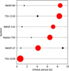 |
Fig. 1 Overview of hot Jupiters (red) with close-by companions (black), including TOI-2109 b. Sizes are to scale. We note that the WASP-47 system also contains a long-period companion that is not shown here. System parameters are taken from Cañas et al. (2019), Wong et al. (2021), Hord et al. (2022), Korth et al. (2023), Maciejewski et al. (2023) and Nascimbeni et al. (2023). |
2 Observations
TOI-2109 was observed by CHEOPS over a total of 31 visits, 8 of which were phase-curve observations, with the rest being transit observations. The details of these observations, including file keys for data access, can be found in Table A.1. These data can be accessed via the DACE (Data and Analysis Center for Exoplanets) website2 of the University of Geneva via the CHEOPS archive3, via the PYCHEOPS Python package (Maxted et al. 2022) using the provided file keys, or at the CDS. We fully processes these data ourselves.
In addition to observations by CHEOPS, TOI-2109 has also been observed in two TESS (Transiting Exoplanet Survey Satellite, Ricker et al. 2015) Sectors, 25 and 52 (Cycle 2 and 4). However, only the latter is available at a cadence of 120 s, with the first being extracted from the full frame images (FFIs), resulting in a cadence of 30 min4. We fit these light curves to derive the mid-transit times.
Furthermore, Wong et al. (2021) made 20 (partial) transit observations with ground-based telescopes5; these include observations from the Fred Lawrence Whipple Observatory with KeplerCam, the Manner Telescope of the University of Louisville, the Maury Lewin Astronomical Observatory, MuS-CAT2 with TCS at Teide Observatory, MuSCAT3 with FTN at Haleakala Observatory, the Wild Boar Remote Observatory, the Grand-Pra Observatory with the RCO, and the Las Cumbres Observatory Global Telescope network using the telescopes of the McDonald observatory, Siding Spring Observatory, South African Astronomical Observatory, and the Cerro Tololo Inter-american Observatory. Aside from photometric observations, Wong et al. (2021) also published a total of 58 measured radial velocities (RVs) from TRES and FIES, contributing 47 (including 28 from transit spectroscopy observations) and 11, respectively. For these data, we use the derived timings and RVs as provided by Wong et al. (2021).
In addition to these data, TOI-2109 was also observed by several cameras of SuperWASP-N (Wide Angle Search for Planets, Pollacco et al. 2006) from 2006 to 2011, giving us early photometry for our orbital-decay analysis. After phase-folding, the transit is clearly visible. We fully processed these data ourselves.
3 Light curves
3.1 Preparation and reduction
We make use of both the standard CHEOPS Data Reduction Pipeline (DRP Version 14.1.2, Hoyer et al. 2020) and PIPE6 (PSF Imagette Photometric Extraction, Brandeker et al., in prep.; Morris et al. 2021b; Szabó et al. 2021; Brandeker et al. 2022), which is complementary to the DRP. In contrast to the DRP’s aperture photometry on subarrays, PIPE makes use of the point-spread function (PSF) photometry from ‘imagettes’ coming from the satellite. There are trade-offs between the two pipelines. PIPE can, amongst other things, deliver shorter-cadence photometry (although not in the case of TOI-2109), provide a better cosmic-ray correction, and deal better with hot pixels and faint targets, and does not require the roll-angle correction necessary in the DRP photometry and originating from CHEOPS’ nadir-locked orbit and rotating field of view. Some drawbacks of using PIPE are related to inaccuracies in the PSF modelling – which is dependent on pointing jitter –, the location on the detector, the temperature of the telescope, and the spectral energy distribution of the target star.
A similar recipe is followed to reduce the DRP and PIPE data. In the case of the DRP data, we use PYCHEOPS for the data handling. We use the ‘DEFAULT’ aperture data and choose the ‘decontaminate’ option when extracting the light curve, which performs a subtraction of the contamination of nearby stars (> 2000 ppm for TOI-2109 b). After this, we clip outliers that deviate by 5σ or more from the mean absolute deviation of the median-smoothed light curve. The next step is to remove data points with high background values. We correct for the ramp effect (Morris et al. 2021a; Fortier et al. 2024) via linear decorrelation against the ‘thermfront2’ sensor data and clip any remaining outliers at 5σ again (this is mostly done to clip remaining outliers in the observed phase curves; the transit observations remain largely unaffected). For the PIPE data, we start by removing the data points flagged by the pipeline and those that show high sky background values. In the next step, we clip the remaining outliers as we did with the DRP data.
For the reduction of the WASP data, we visually inspect all available fields and mask out all fields except 1, 3, 5, 6, and 8 due to bad transit coverage and/or high scatter. Subsequently, we filter out all data points with values of “SIGMA_XS” > 0.03, which is a measure of the root-mean-square (RMS) scatter of the magnitude of all stars in the frame relative to their mean values. This leaves us with 2110 data points that were acquired over a range of 121 days in 2006.
3.2 Light-curve modelling
For modelling of the light curves, we make use of the Transit and Light Curve Modeller (TLCM, Csizmadia 2020). A short description of the setup and the TLCM is given in Harre et al. (2023). We do not fit the gravity darkening parameters, as the planet’s orbit is aligned and thus does not show a modulation of the light curve during transit. For the phase curves, we additionally fit the geometric albedo Ag of the planet, the mass ratio of the star and planet from the ellipsoidal effect q, and the shift of the brightest point on the planetary surface from the sub-stellar point ε using the TLCM Lambertian phase-curve model, which is similar to the process used by Kálmán et al. (2024). This means that only the reflected light component is regarded for the phase-curve fit, which is sufficient for our analysis, as a detailed atmospheric analysis is not within the scope of this paper and will be published elsewhere (Singh et al., in prep.).
In the case of the CHEOPS and TESS data, we firstly completed a combined fit of all the available light curves for each, yielding a phase-curve fit to the CHEOPS DRP dataset, a fit to the CHEOPS PIPE dataset, and a fit to the 2 min cadence TESS data from Sector 52. The roll-angle effect of the CHEOPS photometry is corrected in the case of the DRP data using the following equation, while fitting the roll-angle parameters RA1 to RA6:
 (1)
(1)
where fϕ is the roll-angle component of the fitted model used to decorrelate against the roll-angle of the satellite, and ϕ is the roll-angle value itself.
TLCM uses the following reparametrisation for the limb darkening parameters:
 (2)
(2)
 (3)
(3)
as implemented in Kálmán et al. (2024) with  , and with u1 and u2 being the quadratic limb darkening parameters from Claret (2017) for TESS and Claret (2021) for CHEOPS, respectively. The priors of the phase-curve fits are shown in Table 1 and the results are shown in Table 2. An example of a TLCM fit to the phase curve from the PIPE data reduction is shown in Fig. 2. In addition, we also tried fitting eccentric orbits in all cases, but found no significant improvements in the fits, which is why we decided to only use the solutions of the circular cases for the following fits to the individual transits.
The mid-transit times obtained from the TLCM fits to the individual transit observations from CHEOPS can be found in Table C.1. The remaining mid-transit times from the TESS data, the WASP data and the data published in Wong et al. (2021) can be found in Table C.2. For all of these, the transit shape was fixed to the shape determined from the phase-curve fits. Even though these fits showed good consistency for the derived parameters, we derived the individual transit timings for both CHEOPS data reductions for comparison. Some of the mid-transit timings were biased due to either missing ingress or egress in the observations, which is why they are filtered out and not used in the following analysis steps. This was determined by visually inspecting the light curves and by comparing the timings retrieved from the DRP and PIPE data - if they agreed well within 1σ, we generally accepted them, except if the timing uncertainties were large (>30 s). All individual transits that were modelled are shown in Fig. B.1.
Priors for the TLCM phase-curve fits.
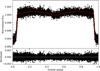 |
Fig. 2 Phase-curve fit (top) of the PIPE data (black) shown with the TLCM’s median solution phase-curve model (red). The residuals of the fit are shown in the bottom plot. |
3.3 Discussion
The phase-curve fits to the CHEOPS and TESS data generally agree for most of the parameters (differences < 1σ or 2σ for most of the fitted parameters between the CHEOPS datasets, except for the orbital period at just over 2σ). Larger deviations between CHEOPS and TESS might be explained by their different wavelength ranges, especially for parameters such as the recovered Rp/R★ values. The impact of CHEOPS’ increased precision over TESS can be mainly seen in the recovered transit parameters. Both of them reach comparable precision in the measurements of the phase-curve parameters due to the increased phase coverage and number of full phase curves that are available during one sector with TESS. Assuming only circular orbits is justified by computing the eccentricity damping timescale (Goldreich & Soter 1966; Patra et al. 2017) as
 (4)
(4)
where with Qp ~ 106, the planetary tidal quality factor of Jupiter, we obtain τe ≈ 1.0 Myr. As the age estimate for this system is  , any primordial eccentricity should be reduced to zero. Nevertheless, a small eccentricity might be induced by the companion (Lee & Peale 2003; Mardling 2007, 2010; Laskar et al. 2012), and obtaining a full phase-curve observation of this planet with for example the Hubble Space Telescope (HST) or the James Webb Space Telescope (JWST, Gardner et al. 2006) would allow the measurement of even small eccentricities with high precision, which would have the added benefit of allowing a precise atmospheric characterisation. A small eccentricity would be strong evidence for the existence of the companion. For a comparison, see the phase curves obtained with JWST for WASP-121 (Mikal-Evans et al. 2023), a star that is relatively similar to TOI-2109, and is also similar in magnitude. Such a phase curve should allow very precise characterisation of the orbital characteristics. In particular, the close proximity of this HJ to its host star and its high equilibrium temperature, in combination with the short orbital period, make observations of this target relatively interesting as well as inexpensive. Apart from just determining the atmospheric composition, signs of an escaping atmosphere could be searched for (see e.g. Dos Santos et al. 2023).
Converting the limb darkening parameters back from A and B (for the values see Table 2) to the standard quadratic limb darkening parameters yields u1,DRP = 0.28 ± 0.17 and u2,DRP = −0.40 ± 0.17, u1,PIPE = 0.28 ± 0.12 and u2,PIPE = −0.07 ± 0.12, and u1,TESS = 0.28 ± 0.20 and u2,TESS = −0.63 ± 0.20. The two solutions coming from the CHEOPS data reductions are in good agreement with each other. However, in all cases, we retrieve negative values for the u2 component. This and the difference between these limb darkening parameters and the theoretical ones from Claret (2021), which are u1,PHX = 0.48 and u2,PHX = 0.20 for the stellar atmosphere models from PHOENIX (Husser et al. 2013), and u1,ATL = 0.31 and u1,ATL = 0.31 for those of ATLAS (Kurucz 1970), might be explained by the fast stellar rotation, which leads to deformation of the star, and hence to gravity darkening. This should impact the obtained limb darkening parameters. Nevertheless, the obtained mid-transit timings should be relatively unaffected by this. Comparing our retrieved limb darkening parameters from the TESS data, we find that they agree with the results of Wong et al. (2021) in terms of the resulting radial intensity profile, again within 2σ, except for the cross-over point and the outermost range, where we only find a 3σ agreement.
Results of the phase-curve fits of TOI-2109 b.
4 Tidal orbital decay
To search for signs of orbital decay in the measured mid-transit timings from the individual fits to the observed transits, we make use of the standard three models – a linear model describing a constant and circular orbit, a quadratic orbital decay model describing the decreasing orbital period, and a sinusoidal model that represents the effect of apsidal precession on the mid-transit timings (see e.g. Patra et al. 2017; Harre et al. 2023).
The model for the mid-transit times of the constant, circular orbit is given in the following:
 (5)
(5)
where N is the individual transit number or epoch, T0 is the reference timing, and P is the orbital period.
The quadratic orbital decay model describes a change in the orbital period of the planet and is given by
 (6)
(6)
where the decay rate is introduced into the timing model as  . This can be converted to the period derivative Ṗ via
 (7)
(7)
This value can subsequently be plugged into the formulation of Goldreich & Soter (1966) to obtain Q′★:
 (8)
(8)
where the tidal factor  , Mp and M★ are the planetary and stellar masses, respectively, R★ is the stellar radius, and a is the semi-major axis of the planetary orbit. The given tidal factor is only valid in the case where the planetary orbital period P is shorter than the stellar rotation period P★. For other configurations, f also depends on the true orbital obliquity ψ of the planet, as is shown in Table 2 of Harre et al. (2023). For TOI-2109 b, we choose the nominal value, although its fast rotation will likely reduce the effect of the tidal decay, depending on which of the rotation periods found in the photometry data by Wong et al. (2021) is the true one.
The sinusoidal model assumes a slightly eccentric orbit, leading to an apsidal precession motion of the planetary orbit. Using the formulations of Giménez & Bastero (1995), we obtain
 (9)
(9)
where Ps is the sidereal period, Pa is the anomalistic period, and ω is the argument of pericentre. The sidereal and anomalistic period are related via:
 (10)
(10)
The argument of pericentre is linearly related to the transit number, and hence with time, via the following equation:
 (11)
(11)
where ω0 is the value of the argument of pericentre at the reference time T0.
From these fits, using a Markov-chain Monte Carlo algorithm via emcee (Foreman-Mackey et al. 2013), we find no significant orbital decay or apsidal precession, and that a linear ephemeris fits the measured mid-transit timings best (see Table 3). Nevertheless, assuming that tidal orbital decay is occurring at the measured rate, and converting the decay rate into the period derivative, we obtain ṖPIPE = (−1.32 ± 1.63) ms yr−1 and ṖDRP = (−1.10 ± 1.69) ms yr−1. This leads to 95% confidence lower limits of Q′★,PIPE > 1.6 × 10⁷ (Q′★,DRP > 1.7 × 10⁷), and for the decay timescalet  , to τPIPE > 12.7 Myr(τDRP > 13.1 Myr).
Even though this target is one of the best candidates for orbital decay in theory, and the early WASP timing that we obtained gives us a long observation baseline, we only measure a decay rate that is in agreement with a constant orbital period. Comparing with the predictions from Wong et al. (2021), which are in the range of ~ 10–740 ms yr−1 for the orbital decay rate, we can clearly rule out the upper end of these predictions. This implies that there is another effect that makes the tidal processes less efficient. One possible explanation could be the fast stellar rotation (v sin i = (81.2 ± 1.6) km s−1); even if it is greater (Prot/ sin i★ ≈ 1.0 d, see Wong et al. 2021) than the orbital period of the HJ, it could still have a negative effect on the efficiency of angular momentum transfer from the planet to the star. The presence of a close-by companion could also affect this. Still, our measured decay rate gives us a constraint on the lower limit of the Q′★ value of TOI-2109 that is not too far from the predicted Q′★ values for F-stars provided by for example Ogilvie & Lin (2007) and Lanza et al. (2011), which are in the range from 105 to 107. We also investigated the impact of atmospheric mass loss on the decay rate of the orbit of the HJ due to its tight orbit. Taking the measurement of the mass-loss rate of KELT-9 b of Ṁ ~ 1012.8±0.3 g s−1 (Wyttenbach et al. 2020) as a first estimate, we find that two to three orders of magnitude more mass loss would be required for it to balance a decay rate of just Ṗ ~ −1 ms yr−1, which is unlikely.
One further complication is related to the apparent sinusoidal TTVs that we observed. Correcting the mid-transit timings for the best-fitting super-period of about 117 d that we found by fitting the sinusoidal model to the data in Sect. 5, we find tentative evidence for orbital decay at a rate of Ṗ = (−5.56 ± 1.62) ms yr−1 at 3σ. This would correspond to 95% confidence lower limits of Q′★ > 8.4 × 10⁶ and τ > 6.6 Myr. We note that this result is sensitive to the applied parameters, because, using the second-best fitting super-period of about 88 d, the result is less significant, with a decreased rate of Ṗ = (−3.53 ± 1.63) ms yr−1 at 2σ. This would lead to lower limits of Q′★ > 1.1 × 10⁷ and τ > 8.6 Myr at 95% confidence.
Furthermore, the gravitational interactions between the two planets, should the second planet exist, might also have an impact on the orbital decay of the HJ. In addition, should this excite a slight eccentricity in the orbit of TOI-2109 b, it would also introduce apsidal precession. Disentangling the two effects is only possible with very long baselines or very precise mid-occultation timings, which we were not able to obtain with sufficient precision for this task from either CHEOPS or TESS. In the future, if a significant orbital decay or apsidal precession signature is detected from continued monitoring – with CHEOPS for example –, JWST should be able to provide the necessary precision with a few occultation observations. Obtaining these would also be relatively inexpensive due to their short duration, and could provide information about the atmosphere.
However, as shown in Harre & Smith (2023), a distant massive planetary companion would also influence the measured mid-transit timings due to the introduction of a light-time effect. Astrometric observations of Gaia’s (Gaia Collaboration 2016) fourth data release will be able to detect such companions, if they are in the right mass and distance range.
Priors and median results of our orbital decay fits for the DRP and PIPE datasets.
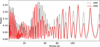 |
Fig. 3 LS periodogram of the transit timing variations measured with CHEOPS for the DRP and PIPE data reductions. |
5 Possible outer companion
Upon closer inspection of the derived CHEOPS mid-transit times, we noticed a sinusoidal variation that is only significant in these data due to the high precision of the CHEOPS photometry. The first thing we did was to create a Lomb-Scargle (LS) periodogram (Zechmeister & Kürster 2009) of the transit timings to find possible periods; see Fig. 3. For both the DRP and PIPE reductions, we obtained multiple peaks of similar power.
The next step was to fit a simple sinusoidal model to the CHEOPS timings to obtain more information about this sinusoidal variation. We employed the following model (see e.g. Lithwick et al. 2012; Ofir et al. 2018) and optimised it using emcee:
 (12)
(12)
where A is the amplitude of the TTVs, Psup is the super-period, and Tsup the super-epoch. To differentiate between the different periods of similar power in the LS periodogram, and to find the best-fitting one, we employed multiple MCMC optimisations of our simple TTV model, trying to find the period that leads to the highest log probability. From this, we determined the parameters of each high-power peak, and sampled them individually for inter-comparison in a further MCMC optimisation (100 walkers and 10 000 steps, with a burn-in phase of 1000 steps). We ensured convergence by checking that the number of steps was at least 50 times the autocorrelation time of all our parameters. We find that Psup ≈ 117 d leads to the lowest BIC value, which is only slightly better (∆BIC = 0.16) than Psup ≈ 88 d. However, both are better than a simple linear model for the mid-transit timings by ∆BIC = 4.0, giving us positive evidence for the apparent TTVs. The final models are shown in Fig. 4 and the respective corner plot in Fig. D.1 for both datasets, which show the good agreement between the two data reductions. This, and the agreement between the orbital decay analyses from the two reductions, demonstrate the consistency of the derived mid-transit timings. Due to this fact, we use only the retrieved PIPE timings for the remainder of our analysis because the roll-angle effect does not need to be accounted for, which should make the fits to the full dataset and the individual timings more reliable.
Due to the relatively high mass of the HJ (5.02 ± 0.75 MJ; see Wong et al. 2021), and the amplitude and period of the apparent TTVs, the companion, if present, must be relatively close by (Agol et al. 2005). As we do not find additional transits in the available photometric data, we argue that planet c has to orbit outside of the orbit of the HJ. Making use of the transit least squares algorithm (Hippke & Heller 2019) to search for additional transits in the residuals of our phase-curve fits, we do not find any significant signals. We searched for orbital periods in the range between 1.0 d and 15.0 d, with the default settings for the search parameters, and the stellar parameters from Wong et al. (2021). Moreover, we also searched for additional transit signals using the détection spécialisée de transits (DST) algorithm (Cabrera et al. 2012), but we did not find any significant evidence of additional planets here either.
The relatively high impact parameter of planet b means that, if planet c is coplanar with planet b, and orbits further out, it will almost certainly not transit the star. In fact, the orbital distance to obtain b = 1.0 would be a = 5.148 R⊙ or P = 1.125 d. In theory, wide ranges of orbital periods and planet masses are possible. In particular, the low precision of the RVs due to the fast stellar rotation is a major drawback in this regard, as it is almost impossible to gain any more information about the system – except for planet b –, leaving only the observed TTVs as a source of information for the possible companion.
To obtain a first estimate of the planet mass and orbital period of the possible outer companion, we used Eq. (33) from Agol et al. (2005). This equation describes the relation between planet masses and TTV amplitude for two planets in an MMR, assuming the more massive planet is transiting. From this, we find masses in the range from 6 to 30 Earth masses for the outer companion, with orbital periods of between 1 and 5 days (i.e. MMRs ranging from 3:2 to 7:1).
5.1 Chaotic and regular orbits
Due to the suspected close proximity of the planet candidate, we first explore regular regions in the mass–period space using REBOUND (Rein & Liu 2012) and its MEGNO (mean exponential growth of nearby orbits; Cincotta & Simó 2000) implementation. MEGNO is a chaos indicator for examining the dynamics of planetary systems.
The setup that we used for the chaos analysis is comprised of a 100 by 100 grid of orbital periods and planetary masses of the outer companion. For each of these grid points, we calculated the MEGNO value. For the setup of the system, we used the parameters given in Wong et al. (2021). Making use of the ‘WHFast’ integrator (Rein & Tamayo 2015), we integrated the system for more than 270 000 orbits of the inner planet. Both circular and eccentric systems were probed for completeness. The result for circular orbits is shown in Fig. 5, and for various eccentricities in Appendix E.
Probing orbital periods of the outer companion from 0.9 to 1.5 days, and planet masses ranging from 1 to 200 Earth masses, we find that there are a few chaotic areas, especially for very close orbits with Pc < 1.0 d. This chaotic area extends up to about 1.05 d for low Mc values. There is another chaotic region between about 1.15 d and 1.19 d for this system. A further, but narrow, chaotic area is present at Pc ≈ 1.39 d, with a few more chaotic regions being found between these areas. However, these are mostly small and do not show the same structure over all examined planetary masses. Beyond orbital periods of 1.5 d, there are no significant chaotic areas in the Mc–Pc space for circular orbits of the two planets.
In the case of eccentric orbits, we find that the innermost regular region gets pushed outwards due to the orbits coming closer together at one point. Depending on the eccentricities used in the simulations, the closest regular area might only be in a narrow area around 1.5 d or even farther out (see Figs. E.1–E.6).
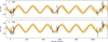 |
Fig. 4 Timing variation plots of the DRP (top) and PIPE (bottom) reductions, showing the lowest BIC models for the two datasets. The blue lines show the median solutions, with the thin orange lines showing random samples drawn from the posterior distribution. The dashed grey lines indicate the best linear models. |
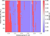 |
Fig. 5 Mass–period MEGNO diagram showing regular and chaotic system configurations for circular orbits of both planets. MEGNO numbers around 2 indicate a regular system (blue), and numbers around 4 indicate a chaotic system (red). The specific MMRs that are within this period range are indicated as vertical dashed lines. |
5.2 TRADES TTV modelling
To model the apparent TTVs in more detail, we employed TRADES7 (TRAnsits and Dynamics of Exoplanetary Systems) (Borsato et al. 2014, 2019), which is a publicly available N-body code designed to model the dynamics of exoplanet systems via TTVs and RVs. There are several approaches to obtaining the final dynamical solution of the examined system; we choose the standard MCMC approach. In two cases, strictly circular or eccentric orbits, we fit for the masses of both planets (Mb, Mc), the orbital periods (Pb, Pc), and their mean anomalies (MAb, MAc). This gives us six free parameters for the circular case. In the case of eccentric orbits, we additionally fit for the eccentricities (eb, ec) and their arguments of pericentre (ωb, ωc) via  and
and  , giving us a total of ten free parameters. The prior intervals and starting values are given in Table 4. The orbital inclination i was fixed to the angle determined by Wong et al. (2021) for both planets, assuming they share the same orbital plane. Due to the scarcity of information that we expect to be able to extract from the available data, we fixed the longitude of the ascending node to Ω = 180° for both planets to reduce the size of the parameter space.
Making use of the pre-optimisať10n that TRADES offers via PyDE8 (Parviainen 2016), with a population size of 128, a generation size of 60 000, and a difference amplification factor and cross-over probability of 0.5, we use this initial optimisation as input for emcee. The latter is run for at least 200 000 steps, using 128 walkers.
We explored circular and eccentric orbits, and in every case, the RVs are also used in the optimisation. Besides these, we explored a few possible MMRs, namely 2:1, 3:1, 5:2, 5:3, 7:2, and 7:3 (ratio of outer to inner period). In these cases, we only allowed a narrow window around the respective resonant orbital period of planet c. All were examined in the cases of circular and eccentric orbits, giving us a total of 12 additional strictly MMR cases. The 3:2 resonance was not probed due to the instability of this close orbital configuration (Pc ≈ 1.0 d), as indicated in Fig. 5. The posterior distributions of the TRADES runs featuring the various MMRs are shown in Figs. 6 and 7, featuring circular and eccentric orbits, respectively.
Comparing the χ2 values of the final results using their maximum a posteriori (MAP) values, we find the best fit for the 5:3 resonance and eccentric orbits with χ2 = 68.4 to the available transit timings from CHEOPS and TESS, and the RVs. Even though this specific setup delivers the best fit, the orbit of planet c with these parameters would likely lead to a chaotic system, with it being on the very edge between regular (‘stable’) and chaotic (‘unstable’). We note that while chaos is linked to instability, regular systems might become unstable after some time. This is owed to the close orbits of the planets in this MMR. The orbital period of Pc = (1.1398 ± 0.0017) d (with P5:3 = 1.121 d being the exact resonance period) and eccentricities of eb = 0.02 and ec = 0.03 cause the orbits to come into proximity, meaning that they may disrupt each other. For the purpose of examining the stability of this configuration, we employed N-body simulations with REBOUND. First, we tested the stability of the MAP solution by simulating the system for 106 yr, which remained stable for this period. Second, we checked the stability of 1000 randomly drawn samples of the posterior for 100 000 orbits of the inner planet (~2000 yr), and only found 3.5% of them to become unstable within this time. The resulting TTV plot of our fit is shown in Fig. 8. The other runs lead mostly to χ2 = 73–88, with the 7:2 resonance for circular orbits leading to the poorest fits, with χ2 ≈ 93. Checking the stability of these solutions for at least 106 yr, we find that the MAP values lead to stable orbits for each configuration. Randomly drawing 1000 samples from each posterior, we find that only six of the resonant configurations have unstable solutions in this sample (including the already mentioned 5:3 MMR in the eccentric case). For the circular 2:1 MMR case, we find that 2 out of 1000 samples become unstable within a time period of 100 000 orbits of the inner planet, and the eccentric 2:1 MMR case leads to 281 unstable configurations. For the eccentric cases, the 5:2 MMR leads to 15, the 7:2 MMR to 1, and the 7:3 MMR to 23 unstable solutions. The remaining configurations remain stable over this time frame.
In the general runs (for the posteriors, see Figs. 9 and 10), without tight constraints on the orbital period of planet c, we obtain the best result in terms of the χ2 value for eccentric orbits, resulting in χ2 = 75.1. The final orbital period of planet c in this case is actually very close to a 4:1 MMR with Pc = 2.677 d, where the exact MMR period would be P4:1 = 2.688 d. The TTV plot is shown in Fig. F.2. It reproduces the super-period of about ~ 117 d that we also find when using the simple sinusoidal model (see Fig. 4). The model allowing circular orbits shows a fit that is worse by ∆χ2 ≈ 3.5, with a final period of the outer companion close to the 7:3 MMR. The respective TTV plot is shown in Fig. F.1.
Priors used in the setup flies for the analysis with TRADES.
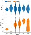 |
Fig. 6 Violin plot of the posterior distributions of the masses of planets ‘b’ (top, blue) and ‘c’ (bottom, orange) derived from the PIPE data in the cases of the MMRs and circular orbits with TRADES. |
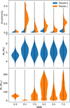 |
Fig. 7 Violin plot of the posterior distributions of the masses and eccentricities from the PIPE data in the cases of the MMRs and eccentric orbits, derived with TRADES. |
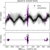 |
Fig. 8 TRADES TTV plot of the best overall fit result, showing a 5:3 MMR and slightly eccentric orbits. Top: fit to the transit timing measurements of TOI-2109 b, including the final model and random samples from the MCMC analysis. Bottom: residuals of the fit. |
5.3 PyTTV analysis
We carry out a set of photo-dynamical analyses modelling the CHEOPS PIPE transit timings, TESS photometry, and the TRES and FIES radial velocities jointly using PyTTV (Korth et al. 2023). The code models the three types of observables (transit photometry, radial velocity measurements, and transit centre time estimates) simultaneously using REBOUND (Rein & Liu 2012; Rein & Spiegel 2015; Tamayo et al. 2020) for dynamical integration and PyTransit (Parviainen 2015; Parviainen & Korth 2020; Parviainen 2020) for transit modelling, and provides posterior densities for the model parameters estimated using MCMC sampling in a standard Bayesian parameter estimation framework. We employ PyTTV in addition to TRADES to make sure that our results are broadly consistent due to the weak constraints that we have on the system.
The model parameters and their priors are listed in Table 5. All the planet parameters except for the log10 mass and radius ratio are defined at a reference time, tref = 2 459 378.46. We set uniform priors on the log masses of the two planets, with ranges designed to help optimisation but not to constrain the posteriors. We set a loosely informative prior on the inner planet’s radius ratio based on the Wong et al. (2021) estimate, and the outer planet’s radius ratio is given a dummy normal prior as the data will not be able to constrain it. We set a normal prior on the inner planet’s transit center and a uniform prior on the outer planet’s mean anomaly (the planets are parameterized differently because the HJ transits and the other does not). We do not constrain the mutual inclinations of the two planets. Instead, we set an informative prior on the inner planet’s impact parameter based on the Wong et al. (2021) estimate of 0.7481 ± 0.0073, and we set a uniform prior on the outer planet impact parameter. The lower limit of the outer planet’s impact parameter prior is justified by the fact that the planet does not transit, and the upper limit was checked not to interfere with the posterior after the MCMC sampling. Finally, we set additional zero-centred half-normal priors on the eccentricities, 𝒩(0.0, 0.023). These priors allow eccentric orbits but bias against high eccentricities.
The analysis begins with a global optimisation using the differential evolution method (Storn & Price 1997; Price et al. 2005) implemented in PyTransit (Parviainen 2015). The optimiser starts with a population of parameter vectors drawn from the model prior, and clumps the population close to the global posterior mode. After the optimisation, we use the clumped parameter vector population to initialise the emcee sampler (Foreman-Mackey et al. 2013), which we then use for MCMC sampling to obtain a sample from the parameter posterior.
We repeat the analysis for the 5:3, 2:1, 7:3, 5:2, 3:1, and 7:2 period commensurability scenarios. For each scenario, we set the outer planet period prior to 𝒩(r × 0.67247414,0.1), where r is the period ratio for the scenario. We present the posterior distributions for the planet masses, orbital inclinations, and orbital eccentricities from the PyTTV analysis in Fig. 11. The Bayesian information criterion (BIC) favours the 3:1 period commensurability scenario, in which there is also a relatively small difference in the orbital inclinations. Looking at the individual likelihoods from the photometry, transit centres, and RVs, the 3:1 scenario is mainly favoured by the improved fit of the RV measurements. Indeed, the photometry and transit centre likelihood distributions corresponding to the posterior parameter distributions largely overlap, as do those for the RV data for all the scenarios other than 3:1.
PyTTV model parameters and priors.
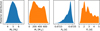 |
Fig. 9 Posterior distributions of the masses and periods for the general run (Pc not constrained to be near a certain MMR) for circular orbits, derived with TRADES. The results for planets b and c are indicated in blue and orange, respectively. |
 |
Fig. 10 Posterior distributions of the eccentricities, masses, and periods for the general run (Pc not constrained to be near a certain MMR) for eccentric orbits, derived with TRADES. The results for planet b and c are indicated in blue and orange, respectively. |
5.4 Discussion of the TTV analysis
As we do not find additional transits in the available photometric data and due to the close proximity of the HJ to its host star, we establish that the companion has to be orbiting outside of the orbit of TOI-2109 b, should it exist. Furthermore, if the orbit of planet c were aligned with that of planet b, it would have to orbit with Pc < 1.125 d to be transiting (which would roughly correspond to a 5:3 MMR), indicating a longer orbital period than this lower limit, which all of our tested cases correspond to. In theory, there are regular orbital solutions interior to the HJ; however, the probability that the inner planet does not transit would be relatively small, requiring a large misalignment with a nearly polar orbit, with the orbital plane having to be aligned almost perfectly perpendicular to our line of sight.
Unfortunately, the fast rotation of the host star hinders the precise measurement of RVs due to the inherent line broadening that this characteristic leads to. This means that it is unlikely that the close companion candidate will be confirmed using this method, even if many observations are taken with high-precision instruments. A major drawback is also the loose constraint on the mass of TOI-2109 b. The dynamical model would benefit from a reduced parameter space in order to better constrain the other fitted parameters. A possible solution for the characterisation of this system could be to obtain at least two phase-curve observations with JWST (see e.g. Mikal-Evans et al. 2023; Bell et al. 2024). This would give us six precise timing measurements (four occultation timings and two transit timings) that, if spread out sufficiently over the phase of a sinusoid, have the potential to massively constrain the parameter space for the dynamical analysis of this system.
The results of our TRADES TTV analysis reveal many possible orbital configurations that could result in the apparent TTVs that have been observed given the loose constraints that we have of the system. Some of the examined cases show poor convergence, which could not always be ensured owing to either the constraints that we enforced in the cases where we examined specific MMRs, or stochastic variations in the pre-optimisation procedure. Checking the stability of the circular orbit MMR solutions, we find that all of them seem to lead to regular systems and are stable for at least 1 Myr using the MAP solutions. However, the 5:3 MMR case leads to a final system configuration and orbital period (Pc = 1.139 d) that is close to the chaotic area but is on the verge of the regular regime, as can be seen in Fig. 5. Nevertheless, we find the MAP solution to be stable for at least 1 Myr using N-body simulations, and all of the 1000 randomly drawn samples of the posterior to be stable for 100 000 orbits of the HJ. The overall best-fitting result is obtained from the 5:3 MMR case, where we allow non-zero eccentricities. According to REBOUND simulations using the final MAP parameters from TRADES, we obtain stable orbits for at least 1 Myr using N-body simulations. Even the grand majority of the 1000 randomly drawn samples of the posterior are stable for 100000 orbits of the inner planet. However, the regular area is relatively tight within the mean-longitude-period space according to the MEGNO indicator. Nevertheless, this is our overall best-fitting result.
The best-fitting result that we obtain from our general circular TRADES fit (see Fig. F.1) shows a relatively high-frequency modulation of the TTVs, with some of the chains reproducing the trend that is seen in Fig. 8. Our result that allows eccentric orbits in the general case (see Fig. F.2) is close to a4:1 MMR and also reproduces the TTV super-period of ~ 117 d that we find to be the best fit using the simple sinusoidal model (see Figs. 4 and D.1). Even if we cannot solve the system with the available data, we see a good agreement between the two approaches, which is evidence that the apparent sinusoidal TTVs are real. In theory, TTVs of this amplitude could be caused by starspot crossing events (Ioannidis et al. 2016), but this seems quite unlikely in this case due to the star being an F-type star, and given the very low probability that this effect will occur consistently over three observing seasons. In addition, we do not find signs of starspot crossings in the transits that we captured with CHEOPS.
Investigating the stability of the remaining cases that we examined, we find that the individual MAP solutions are all stable for 1 Myr, as tested with REBOUND, and as has been seen for the circular orbits. When randomly drawing samples from the posterior and testing their stability, we also see that most solutions are stable for 100000 orbits of the HJ (see Sect. 5.2). For the general runs, we observe that in both cases, that is with circular and eccentric orbits, all tested solutions lead to stable systems over the examined time frames.
Regarding the PyTTV analysis, we find the 3:1 MMR to lead to the best fit, mainly due to the RV data. This means that the RV data may provide some evidence of planet c, though this evidence remains tentative at best, due to the large RV uncertainties, and the TTVs have the highest impact in the fitting process. Before comparison of these results with those of TRADES, we first of all have to note the different approaches that were chosen for the two codes. While we are using the same datasets in both cases, we fit for more parameters using PyTTV due to its faster and more flexible approach, where the inclusion of the orbital inclination in particular might have an impact on the results. Here, we also only focused on the specific MMRs in cases where we allow non-zero eccentricities. Comparing the results (Figs. 7 and 11), we can see the effect that the PyTTV photo-dynamical model has on the final fits by inspecting the final eccentricities. The PyTTV model achieves better convergence due to it being able to better break the mass-eccentricity degeneracies that can be seen for the TRADES equivalents of the runs. Lower eccentricities should lead to more stable systems, especially for such tight systems; while in the case of TRADES, we find greater possible eccentricities for planet c, especially in the 2:1, 5:2, and 7:2 MMRs cases, which may explain the differences in the posterior mass ranges. Other than this, the posteriors mostly agree with each other and show similar trends; the remaining difference can be explained by the inclinations of planet c in the PyTTV runs.
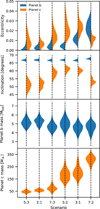 |
Fig. 11 Posterior densities for the planet masses, orbital inclinations, and orbital eccentricities obtained from the PyTTV analysis for the six considered period commensurability scenarios. |
6 Conclusions
By examining newly obtained CHEOPS photometry of the TOI-2109 system, we discovered sinusoidal transit-timing variations (TTVs) while searching for signs of tidal orbital decay. We also find tentative evidence for this latter phenomenon when correcting the mid-transit timings using a simple sinusoidal model that best describes the TTVs. As we are unable to find additional transits in the available photometry, we conclude that the candidate planet c must orbit outside of the orbit of TOI-2109 b with a period of greater than Pc ≈ 1.13 d owing to the high impact parameter and the orbital inclination of planet b, assuming co-planar orbits. Probing the apparent TTVs using a simple sine model, we found that two super-periods (Psup ≈ 88 d and Psup ≈ 117 d) fit the observations best when compared to a simple linear model, which is positive evidence (ΔBIC = 4) for the authenticity of the TTVs.
Applying the N-body code TRADES (Borsato et al. 2014, 2019) to our dataset (for other examples see e.g. Malavolta et al. 2017; Nespral et al. 2017; Borsato et al. 2019, 2024; Nascimbeni et al. 2023), we find that the best-fitting solution corresponds to a 5:3 mean-motion resonance (MMR) with Pc = (1.1398 ± 0.0017) d and slight eccentricities. This solution is stable for at least 1 Myr according to our N-body simulations using REBOUND. From general, non-strictly MMR fits, we find orbital periods of the outer candidate companion of about Pc ≈ 1.57 d (close to a 7:3 MMR) in the circular case and Pc ≈ 2.67 d (close to a 4:1 MMR) in the eccentric case. The free eccentric fit solutions are compatible with the best-fitting super-period that we found during our investigation of the TTVs with the simple sinusoidal model. Furthermore, even some of the chains of the circular general fit reproduce our best-fitting model of the 5:3 MMR with eccentricities. In addition to our TTV analysis with TRADES, we also made use of PyTTV (Korth et al. 2023). While we do not find the same preference for the 5:3 MMR, we find a slight preference for the 3:1 MMR and similar posterior distributions between the codes in general. Differences between the two can be explained by the different approach that was chosen in the modelling, with more parameters being included in PyTTV that were fixed in the TRADES analysis to achieve faster convergence. Owing to the low amplitude of the TTVs and the quality of the RV measurements caused by the fast rotation of the stellar host, we cannot yet fully confirm the new planetary candidate, or which of the models is preferred overall. More precise timing measurements are necessary in this regard. Continued monitoring with CHEOPS would be a possible solution and would also support the search for orbital decay, as the TESS observations carried out so far are not sufficiently precise in terms of the retrieved mid-transit timings.
Hubble Space Telescope or JWST observations of this system would not only allow atmospheric characterisation of this short-period ultra-hot Jupiter, but would give us the opportunity to obtain very precise timing measurements, even if only a few were obtained. Spread out over the phase of the possible sinusoids, six precise timings from two phase-curve observations (four occultation timings and two transit timings) could precisely constrain the parameter space, and should enable us to fully confirm this planet and better determine its characteristics. Due to the close orbit, these observations would be relatively inexpensive in terms of observation time.
Confirming the existence of the planet candidate would add TOI-2109 to the rare class of HJs with close companions and would make it only the second of these systems to host an outer companion, after the WASP-47 system (Becker et al. 2015; Almenara et al. 2016; Neveu-VanMalle et al. 2016; Vanderburg et al. 2017; Nascimbeni et al. 2023).
Data availability
Table C.2, as well as the raw and detrended CHEOPS data from both, the DRP and PIPE data reductions, are available in electronic form at the CDS via anonymous ftp to cdsarc.cds.unistra.fr (130.79.128.5) or via https://cdsarc.cds.unistra.fr/viz-bin/cat/J/A+A/692/A254.
Acknowledgements
The authors thank the anonymous referee for their helpful comments, which helped to improve the clarity of the manuscript. CHEOPS is an ESA mission in partnership with Switzerland with important contributions to the payload and the ground segment from Austria, Belgium, France, Germany, Hungary, Italy, Portugal, Spain, Sweden, and the United Kingdom. The CHEOPS Consortium would like to gratefully acknowledge the support received by all the agencies, offices, universities, and industries involved. Their flexibility and willingness to explore new approaches were essential to the success of this mission. CHEOPS data analysed in this article will be made available in the CHEOPS mission archive (https://cheops.unige.ch/archive_browser/). JVH is funded by the DFG priority programme SPP 1992 “Exploring the Diversity of Extrasolar Planets (SM 486/2-1)”. S.C.C.B. acknowledges support from FCT through FCT contracts nr. IF/01312/2014/CP1215/CT0004. LBo, GBr, VNa, IPa, GPi, RRa, GSc, VSi, and TZi acknowledge support from CHEOPS ASI-INAF agreement no. 2019-29-HH.0. ABr was supported by the SNSA. ACC acknowledges support from STFC consolidated grant number ST/V000861/1, and UKSA grant number ST/X002217/1. ML acknowledges support of the Swiss National Science Foundation under grant number PCEFP2_194576. TWi acknowledges support from the UKSA and the University of Warwick. ACMC acknowledges support from the FCT, Portugal, through the CFisUC projects UIDB/04564/2020 and UIDP/04564/2020, with DOI identifiers 10.54499/UIDB/04564/2020 and 10.54499/UIDP/04564/2020, respectively. YAl acknowledges support from the Swiss National Science Foundation (SNSF) under grant 200020_192038. We acknowledge financial support from the Agencia Estatal de Investigación of the Ministerio de Ciencia e Innovación MCIN/AEI/10.13039/501100011033 and the ERDF “A way of making Europe” through projects PID2019-107061GB-C61, PID2019-107061GB-C66, PID2021-125627OB-C31, and PID2021-125627OB-C32, from the Centre of Excellence “Severo Ochoa” award to the Instituto de Astrofísica de Canarias (CEX2019-000920-S), from the Centre of Excellence “María de Maeztu” award to the Institut de Ciències de l’Espai (CEX2020-001058-M), and from the Generalitat de Catalunya/CERCA programme. We acknowledge financial support from the Agencia Estatal de Investigación of the Ministerio de Ciencia e Innovación MCIN/AEI/10.13039/501100011033 and the ERDF “A way of making Europe” through projects PID2019-107061GB-C61, PID2019-107061GB-C66, PID2021-125627OB-C31, and PID2021-125627OB-C32, from the Centre of Excellence “Severo Ochoa” award to the Instituto de Astrofísica de Canarias (CEX2019-000920-S), from the Centre of Excellence “María de Maeztu” award to the Institut de Ciències de l’Espai (CEX2020-001058-M), and from the Generalitat de Catalunya/CERCA programme. C.B. acknowledges support from the Swiss Space Office through the ESA PRODEX program. This work has been carried out within the framework of the NCCR PlanetS supported by the Swiss National Science Foundation under grants 51NF40_182901 and 51NF40_205606. P.E.C. is funded by the Austrian Science Fund (FWF) Erwin Schroedinger Fellowship, program J4595-N. This project was supported by the CNES. The Belgian participation to CHEOPS has been supported by the Belgian Federal Science Policy Office (BELSPO) in the framework of the PRODEX Program, and by the University of Liège through an ARC grant for Concerted Research Actions financed by the Wallonia-Brussels Federation. L.D. thanks the Belgian Federal Science Policy Office (BELSPO) for the provision of financial support in the framework of the PRODEX Programme of the European Space Agency (ESA) under contract number 4000142531. This work was supported by FCT – Fundação para a Ciência e a Tecnologia through national funds and by FEDER through COMPETE2020 through the research grants UIDB/04434/2020, UIDP/04434/2020, 2022.06962.PTDC. O.D.S.D. is supported in the form of work contract (DL 57/2016/CP1364/CT0004) funded by national funds through FCT. B.-O. D. acknowledges support from the Swiss State Secretariat for Education, Research and Innovation (SERI) under contract number MB22.00046. This project has received funding from the Swiss National Science Foundation for project 200021_200726. It has also been carried out within the framework of the National Centre of Competence in Research PlanetS supported by the Swiss National Science Foundation under grant 51NF40_205606. The authors acknowledge the financial support of the SNSF. MF and CMP gratefully acknowledge the support of the Swedish National Space Agency (DNR 65/19, 174/18). DG gratefully acknowledges financial support from the CRT foundation under Grant No. 2018.2323 “Gaseousor rocky? Unveiling the nature of small worlds”. M.G. is an F.R.S.-FNRS Senior Research Associate. MNG is the ESA CHEOPS Project Scientist and Mission Representative, and as such also responsible for the Guest Observers (GO) Programme. MNG does not relay proprietary information between the GO and Guaranteed Time Observation (GTO) Programmes, and does not decide on the definition and target selection of the GTO Programme. CHe acknowledges support from the European Union H2020-MSCA-ITN-2019 under Grant Agreement no. 860470 (CHAMELEON). KGI is the ESA CHEOPS Project Scientist and is responsible for the ESA CHEOPS Guest Observers Programme. She does not participate in, or contribute to, the definition of the Guaranteed Time Programme of the CHEOPS mission through which observations described in this paper have been taken, nor to any aspect of target selection for the programme. K.W.F.L. was supported by Deutsche Forschungsgemeinschaft grants RA714/14-1 within the DFG Schwerpunkt SPP 1992, Exploring the Diversity of Extrasolar Planets. This work was granted access to the HPC resources of MesoPSL financed by the Region Ile de France and the project Equip@Meso (reference ANR-10-EQPX-29-01) of the programme Investissements d’Avenir supervised by the Agence Nationale pour la Recherche. PM acknowledges support from STFC research grant number ST/R000638/1. This work was also partially supported by a grant from the Simons Foundation (PI Queloz, grant number 327127). NCSa acknowledges funding by the European Union (ERC, FIERCE, 101052347). Views and opinions expressed are however those of the author(s) only and do not necessarily reflect those of the European Union or the European Research Council. Neither the European Union nor the granting authority can be held responsible for them. A. S. acknowledges support from the Swiss Space Office through the ESA PRODEX program. S.G.S. acknowledge support from FCT through FCT contract nr. CEECIND/00826/2018 and POPH/FSE (EC). The Portuguese team thanks the Portuguese Space Agency for the provision of financial support in the framework of the PRODEX Programme of the European Space Agency (ESA) under contract number 4000142255. GyMSz acknowledges the support of the Hungarian National Research, Development and Innovation Office (NKFIH) grant K-125015, a a PRODEX Experiment Agreement No. 4000137122, the Lendület LP2018-7/2021 grant of the Hungarian Academy of Science and the support of the city of Szombathely. V.V.G. is an F.R.S-FNRS Research Associate. JV acknowledges support from the Swiss National Science Foundation (SNSF) under grant PZ00P2_208945. NAW acknowledges UKSA grant ST/R004838/1. This work made use of the Python libraries NumPy (Harris et al. 2020), Matplotlib (Hunter 2007), corner (Foreman-Mackey 2016), and Astropy (Astropy Collaboration 2022).
Appendix A CHEOPS observations log
CHEOPS observations of TOI-2109.
Appendix B Individual transit plots
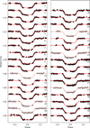 |
Fig. B.1 All individual transits from the PIPE data (black) that were fitted using TLCM with the respective transit models (red). The numbers below each transit light curve indicate the number of the corresponding visit, see Table A.1. Duplications in visit number refer to the first and second transit in a phase-curve observation. If the resulting transit timings were not used in the TTV analysis, they are greyed out. |
Appendix C Retrieved mid−transit timings
Mid-transit times of TOI-2109 b, retrieved from the CHEOPS DRP and PIPE data reductions.
Mid-transit times of TOI-2109 b, retrieved from the ground-based data published in Wong et al. (2021), WASP and TESS.
Appendix D Sine fit corner plot
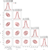 |
Fig. D.1 Final corner plot of the fit of the simple sine model (Eq. 12) to the mid-transit timings, measured with CHEOPS using the DRP and PIPE reductions. The dashed lines indicate the 1σ errors around the median value. The contours show the 0.5σ, lσ, 1.5σ and 2σ levels. T0 is given in BJDTDB − 2450000. |
Appendix E Additional MEGNO eccentricity plots
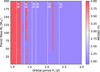 |
Fig. E.1 MEGNO plot of the TOI-2109 system for a circular orbit of the hot Jupiter and a slightly eccentric orbit of planet c (ec = 0.05), for 270 000 orbits of the inner planet. |
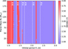 |
Fig. E.2 MEGNO plot of TOI-2109 for eccentric orbits of both planets with eb = 0.03 and ec = 0.05, computed for 270 000 orbits of the inner planet. |
 |
Fig. E.3 MEGNO plot of the TOI-2109 system for a circular orbit of the hot Jupiter and a moderately eccentric orbit of planet c (ec = 0.15), for 270 000 orbits of the inner planet. |
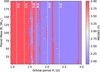 |
Fig. E.4 MEGNO plot of TOI-2109 for eccentric orbits of both planets with eb = 0.03 and ec = 0.15, computed for 270 000 orbits of the inner planet. |
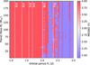 |
Fig. E.5 MEGNO plot of the TOI-2109 system for a circular orbit of the hot Jupiter and an eccentric orbit of planet c (ec = 0.25), for 270 000 orbits of the inner planet. |
 |
Fig. E.6 MEGNO plot of TOI-2109 for eccentric orbits of both planets with eb = 0.03 and ec = 0.25, computed for 270 000 orbits of the inner planet. |
Appendix F Additional TRADESTTV plots
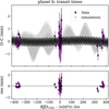 |
Fig. F.1 TRADES TTV plot of the general circular orbit fit. Top: Fit to the transit timing measurements of TOI-2109 b, including the final MAP model and random samples from the MCMC analysis. Bottom: Residuals of the fit. |
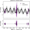 |
Fig. F.2 TRADES TTV plot of the general eccentric orbit fit. Top: Fit to the transit timing measurements of TOI-2109 b, including the final MAP model and random samples from the MCMC analysis. Bottom: Residuals of the fit. |
References
- Agol, E., Steffen, J., Sari, R., & Clarkson, W. 2005, MNRAS, 359, 567 [Google Scholar]
- Albrecht, S. H., Marcussen, M. L., Winn, J. N., Dawson, R. I., & Knudstrup, E. 2021, ApJ, 916, L1 [NASA ADS] [CrossRef] [Google Scholar]
- Albrecht, S. H., Dawson, R. I., & Winn, J. N. 2022, PASP, 134, 082001 [NASA ADS] [CrossRef] [Google Scholar]
- Almenara, J. M., Díaz, R. F., Bonfils, X., & Udry, S. 2016, A&A, 595, L5 [NASA ADS] [CrossRef] [EDP Sciences] [Google Scholar]
- Anderson, D. R., Collier Cameron, A., Delrez, L., et al. 2014, MNRAS, 445, 1114 [NASA ADS] [CrossRef] [Google Scholar]
- Astropy Collaboration (Price-Whelan, A. M., et al.) 2022, ApJ, 935, 167 [NASA ADS] [CrossRef] [Google Scholar]
- Barros, S. C. C., Akinsanmi, B., Boué, G., et al. 2022, A&A, 657, A52 [NASA ADS] [CrossRef] [EDP Sciences] [Google Scholar]
- Becker, J. C., Vanderburg, A., Adams, F. C., Rappaport, S. A., & Schwengeler, H. M. 2015, ApJ, 812, L18 [NASA ADS] [CrossRef] [Google Scholar]
- Bell, T. J., Crouzet, N., Cubillos, P. E., et al. 2024, Nat. Astron., 8, 879 [Google Scholar]
- Benz, W., Broeg, C., Fortier, A., et al. 2021, Exp. Astron., 51, 109 [Google Scholar]
- Borsato, L., Marzari, F., Nascimbeni, V., et al. 2014, A&A, 571, A38 [NASA ADS] [CrossRef] [EDP Sciences] [Google Scholar]
- Borsato, L., Malavolta, L., Piotto, G., et al. 2019, MNRAS, 484, 3233 [NASA ADS] [CrossRef] [Google Scholar]
- Borsato, L., Degen, D., Leleu, A., et al. 2024, A&A, 689, A52 [NASA ADS] [CrossRef] [EDP Sciences] [Google Scholar]
- Boué, G., & Efroimsky, M. 2019, Celest. Mech. Dyn. Astron., 131, 30 [CrossRef] [Google Scholar]
- Brandeker, A., Heng, K., Lendl, M., et al. 2022, A&A, 659, L4 [NASA ADS] [CrossRef] [EDP Sciences] [Google Scholar]
- Cañas, C. I., Wang, S., Mahadevan, S., et al. 2019, ApJ, 870, L17 [CrossRef] [Google Scholar]
- Cabrera, J., Csizmadia, S., Erikson, A., Rauer, H., & Kirste, S. 2012, A&A, 548, A44 [NASA ADS] [CrossRef] [EDP Sciences] [Google Scholar]
- Cincotta, P. M., & Simó, C. 2000, A&AS, 147, 205 [NASA ADS] [CrossRef] [EDP Sciences] [Google Scholar]
- Claret, A. 2017, A&A, 600, A30 [NASA ADS] [CrossRef] [EDP Sciences] [Google Scholar]
- Claret, A. 2021, RNAAS, 5, 13 [NASA ADS] [Google Scholar]
- Collier Cameron, A., & Jardine, M. 2018, MNRAS, 476, 2542 [Google Scholar]
- Counselman I., Charles C., 1973, ApJ, 180, 307 [NASA ADS] [CrossRef] [Google Scholar]
- Csizmadia, S. 2020, MNRAS, 496, 4442 [Google Scholar]
- Dawson, R. I., & Johnson, J. A. 2018, ARA&A, 56, 175 [Google Scholar]
- Deline, A., Hooton, M. J., Lendl, M., et al. 2022, A&A, 659, A74 [NASA ADS] [CrossRef] [EDP Sciences] [Google Scholar]
- Dos Santos, L. A., Alam, M. K., Espinoza, N., & Vissapragada, S. 2023, AJ, 165, 244 [NASA ADS] [CrossRef] [Google Scholar]
- Foreman-Mackey, D. 2016, J. Open Source Softw., 1, 24 [Google Scholar]
- Foreman-Mackey, D., Hogg, D. W., Lang, D., & Goodman, J. 2013, PASP, 125, 306 [Google Scholar]
- Fortier, A., Simon, A. E., Broeg, C., et al. 2024, A&A, 687, A302 [NASA ADS] [CrossRef] [EDP Sciences] [Google Scholar]
- Gaia Collaboration (Prusti, T., et al.) 2016, A&A, 595, A1 [NASA ADS] [CrossRef] [EDP Sciences] [Google Scholar]
- Galazutdinov, G. A., Baluev, R. V., Valyavin, G., et al. 2023, MNRAS, 526, L111 [Google Scholar]
- Gardner, J. P., Mather, J. C., Clampin, M., et al. 2006, Space Sci. Rev., 123, 485 [Google Scholar]
- Gaudi, B. S., Stassun, K. G., Collins, K. A., et al. 2017, Nature, 546, 514 [NASA ADS] [Google Scholar]
- Gillon, M., Triaud, A. H. M. J., Demory, B.-O., et al. 2017, Nature, 542, 456 [NASA ADS] [CrossRef] [Google Scholar]
- Giménez, A., & Bastero, M. 1995, Ap&SS, 226, 99 [Google Scholar]
- Goldreich, P., & Soter, S. 1966, Icarus, 5, 375 [Google Scholar]
- Grimm, S. L., Demory, B.-O., Gillon, M., et al. 2018, A&A, 613, A68 [NASA ADS] [CrossRef] [EDP Sciences] [Google Scholar]
- Grunblatt, S. K., Saunders, N., Sun, M., et al. 2022, AJ, 163, 120 [NASA ADS] [CrossRef] [Google Scholar]
- Hadden, S., & Lithwick, Y. 2014, ApJ, 787, 80 [Google Scholar]
- Hadden, S., & Lithwick, Y. 2017, AJ, 154, 5 [Google Scholar]
- Harre, J.-V., & Smith, A. M. S. 2023, Universe, 9, 506 [Google Scholar]
- Harre, J. V., Smith, A. M. S., Barros, S. C. C., et al. 2023, A&A, 669, A124 [NASA ADS] [CrossRef] [EDP Sciences] [Google Scholar]
- Harris, C. R., Millman, K. J., van der Walt, S. J., et al. 2020, Nature, 585, 357 [NASA ADS] [CrossRef] [Google Scholar]
- Hébrard, G., Díaz, R. F., Correia, A. C. M., et al. 2020, A&A, 640, A32 [EDP Sciences] [Google Scholar]
- Hellier, C., Anderson, D. R., Collier Cameron, A., et al. 2012, MNRAS, 426, 739 [NASA ADS] [CrossRef] [Google Scholar]
- Hellier, C., Anderson, D. R., Collier Cameron, A., et al. 2017, MNRAS, 465, 3693 [NASA ADS] [CrossRef] [Google Scholar]
- Hippke, M., & Heller, R. 2019, A&A, 623, A39 [NASA ADS] [CrossRef] [EDP Sciences] [Google Scholar]
- Holman, M. J., Fabrycky, D. C., Ragozzine, D., et al. 2010, Science, 330, 51 [Google Scholar]
- Hord, B. J., Colón, K. D., Berger, T. A., et al. 2022, AJ, 164, 13 [NASA ADS] [CrossRef] [Google Scholar]
- Hoyer, S., Guterman, P., Demangeon, O., et al. 2020, A&A, 635, A24 [NASA ADS] [CrossRef] [EDP Sciences] [Google Scholar]
- Huang, C. X., Quinn, S. N., Vanderburg, A., et al. 2020, ApJ, 892, L7 [CrossRef] [Google Scholar]
- Hunter, J. D. 2007, Comput. Sci. Eng., 9, 90 [NASA ADS] [CrossRef] [Google Scholar]
- Husnoo, N., Pont, F., Mazeh, T., et al. 2012, MNRAS, 422, 3151 [NASA ADS] [CrossRef] [Google Scholar]
- Husser, T. O., Wende-von Berg, S., Dreizler, S., et al. 2013, A&A, 553, A6 [NASA ADS] [CrossRef] [EDP Sciences] [Google Scholar]
- Hut, P. 1981, A&A, 99, 126 [NASA ADS] [Google Scholar]
- Ioannidis, P., Huber, K. F., & Schmitt, J. H. M. M. 2016, A&A, 585, A72 [NASA ADS] [CrossRef] [EDP Sciences] [Google Scholar]
- Ivshina, E. S., & Winn, J. N. 2022, ApJS, 259, 62 [CrossRef] [Google Scholar]
- Jackson, B., Greenberg, R., & Barnes, R. 2008, ApJ, 678, 1396 [Google Scholar]
- Jones, K., Morris, B. M., Demory, B. O., et al. 2022, A&A, 666, A118 [NASA ADS] [CrossRef] [EDP Sciences] [Google Scholar]
- Kálmán, S., Derekas, A., Csizmadia, S., et al. 2024, A&A, 687, A144 [NASA ADS] [CrossRef] [EDP Sciences] [Google Scholar]
- Kipping, D. M. 2013, MNRAS, 435, 2152 [Google Scholar]
- Korth, J., Gandolfi, D., Šubjak, J., et al. 2023, A&A, 675, A115 [NASA ADS] [CrossRef] [EDP Sciences] [Google Scholar]
- Korth, J., Chaturvedi, P., Parviainen, H., et al. 2024, ApJ, 971, L28 [NASA ADS] [CrossRef] [Google Scholar]
- Kraft, R. P. 1967, ApJ, 150, 551 [Google Scholar]
- Kurucz, R. L. 1970, SAO Special Report, 309 [Google Scholar]
- Lanza, A. F., Damiani, C., & Gandolfi, D. 2011, A&A, 529, A50 [NASA ADS] [CrossRef] [EDP Sciences] [Google Scholar]
- Laskar, J., Boué, G., & Correia, A. C. M. 2012, A&A, 538, A105 [NASA ADS] [CrossRef] [EDP Sciences] [Google Scholar]
- Lee, M. H., & Peale, S. J. 2003, ApJ, 592, 1201 [Google Scholar]
- Leleu, A., Alibert, Y., Hara, N. C., et al. 2021, A&A, 649, A26 [NASA ADS] [CrossRef] [EDP Sciences] [Google Scholar]
- Lendl, M., Csizmadia, S., Deline, A., et al. 2020, A&A, 643, A94 [EDP Sciences] [Google Scholar]
- Lithwick, Y., Xie, J., &Wu, Y. 2012, ApJ, 761, 122 [NASA ADS] [CrossRef] [Google Scholar]
- MacDonald, M. G., Ragozzine, D., Fabrycky, D. C., et al. 2016, AJ, 152, 105 [Google Scholar]
- Maciejewski, G., Knutson, H. A., Howard, A. W., et al. 2020, Acta Astron., 70, 1 [NASA ADS] [Google Scholar]
- Maciejewski, G., Golonka, J., Loboda, W., et al. 2023, MNRAS, 525, L43 [CrossRef] [Google Scholar]
- Malavolta, L., Borsato, L., Granata, V., et al. 2017, AJ, 153, 224 [NASA ADS] [CrossRef] [Google Scholar]
- Mantovan, G., Malavolta, L., Desidera, S., et al. 2024, A&A, 682, A129 [NASA ADS] [CrossRef] [EDP Sciences] [Google Scholar]
- Mardling, R. A. 2007, MNRAS, 382, 1768 [NASA ADS] [Google Scholar]
- Mardling, R. A. 2010, MNRAS, 407, 1048 [Google Scholar]
- Maxted, P. F. L., Ehrenreich, D., Wilson, T. G., et al. 2022, MNRAS, 514, 77 [NASA ADS] [CrossRef] [Google Scholar]
- Meibom, S., & Mathieu, R. D. 2005, ApJ, 620, 970 [Google Scholar]
- Mikal-Evans, T., Sing, D. K., Dong, J., et al. 2023, ApJ, 943, L17 [CrossRef] [Google Scholar]
- Morris, B. M., Delrez, L., Brandeker, A., et al. 2021a, A&A, 653, A173 [NASA ADS] [CrossRef] [EDP Sciences] [Google Scholar]
- Morris, B. M., Heng, K., Brandeker, A., Swan, A., & Lendl, M. 2021b, A&A, 651, L12 [NASA ADS] [CrossRef] [EDP Sciences] [Google Scholar]
- Nascimbeni, V., Borsato, L., Zingales, T., et al. 2023, A&A, 673, A42 [NASA ADS] [CrossRef] [EDP Sciences] [Google Scholar]
- Nespral, D., Gandolfi, D., Deeg, H. J., et al. 2017, A&A, 601, A128 [NASA ADS] [CrossRef] [EDP Sciences] [Google Scholar]
- Neveu-VanMalle, M., Queloz, D., Anderson, D. R., et al. 2016, A&A, 586, A93 [NASA ADS] [CrossRef] [EDP Sciences] [Google Scholar]
- Ofir, A., Xie, J.-W., Jiang, C.-F., Sari, R., & Aharonson, O. 2018, ApJS, 234, 9 [CrossRef] [Google Scholar]
- Ogilvie, G. I. 2014, ARA&A, 52, 171 [Google Scholar]
- Ogilvie, G. I., & Lin, D. N. C. 2007, ApJ, 661, 1180 [Google Scholar]
- Parviainen, H. 2015, MNRAS, 450, 3233 [Google Scholar]
- Parviainen, H. 2016, PyDE: v1.5 [Google Scholar]
- Parviainen, H. 2020, MNRAS, 499, 1633 [NASA ADS] [CrossRef] [Google Scholar]
- Parviainen, H., & Korth, J. 2020, MNRAS, 499, 3356 [NASA ADS] [CrossRef] [Google Scholar]
- Patra, K. C., Winn, J. N., Holman, M. J., et al. 2017, AJ, 154, 4 [Google Scholar]
- Patra, K. C., Winn, J. N., Holman, M. J., et al. 2020, AJ, 159, 150 [NASA ADS] [CrossRef] [Google Scholar]
- Penev, K., & Sasselov, D. 2011, ApJ, 731, 67 [NASA ADS] [CrossRef] [Google Scholar]
- Penev, K., Jackson, B., Spada, F., & Thom, N. 2012, ApJ, 751, 96 [NASA ADS] [CrossRef] [Google Scholar]
- Penev, K., Bouma, L. G., Winn, J. N., & Hartman, J. D. 2018, AJ, 155, 165 [NASA ADS] [CrossRef] [Google Scholar]
- Pollacco, D. L., Skillen, I., Collier Cameron, A., et al. 2006, PASP, 118, 1407 [NASA ADS] [CrossRef] [Google Scholar]
- Poon, S. T. S., Nelson, R. P., & Coleman, G. A. L. 2021, MNRAS, 505, 2500 [NASA ADS] [CrossRef] [Google Scholar]
- Price, K., Storn, R., & Lampinen, J. 2005, Differential Evolution (Berlin: Springer) [Google Scholar]
- Rasio, F. A., Tout, C. A., Lubow, S. H., & Livio, M. 1996, ApJ, 470, 1187 [Google Scholar]
- Rein, H., & Liu, S. F. 2012, A&A, 537, A128 [NASA ADS] [CrossRef] [EDP Sciences] [Google Scholar]
- Rein, H., & Spiegel, D. S. 2015, MNRAS, 446, 1424 [Google Scholar]
- Rein, H., & Tamayo, D. 2015, MNRAS, 452, 376 [Google Scholar]
- Rice, M., Wang, S., & Laughlin, G. 2022, ApJ, 926, L17 [NASA ADS] [CrossRef] [Google Scholar]
- Ricker, G. R., Winn, J. N., Vanderspek, R., et al. 2015, J. Astron. Telesc. Instrum. Syst., 1, 014003 [Google Scholar]
- Rosário, N. M., Barros, S. C. C., Demangeon, O. D. S., & Santos, N. C. 2022, A&A, 668, A114 [NASA ADS] [CrossRef] [EDP Sciences] [Google Scholar]
- Sha, L., Vanderburg, A. M., Huang, C. X., et al. 2023, MNRAS, 524, 1113 [NASA ADS] [CrossRef] [Google Scholar]
- Storn, R., & Price, K. 1997, J. Glob. Optim., 11, 341 [Google Scholar]
- Szabó, G. M., Gandolfi, D., Brandeker, A., et al. 2021, A&A, 654, A159 [NASA ADS] [CrossRef] [EDP Sciences] [Google Scholar]
- Tamayo, D., Rein, H., Shi, P., & Hernandez, D. M. 2020, MNRAS, 491, 2885 [NASA ADS] [CrossRef] [Google Scholar]
- Thompson, S. E., Coughlin, J. L., Hoffman, K., et al. 2018, ApJS, 235, 38 [NASA ADS] [CrossRef] [Google Scholar]
- Vanderburg, A., Becker, J. C., Buchhave, L. A., et al. 2017, AJ, 154, 237 [NASA ADS] [CrossRef] [Google Scholar]
- Vissapragada, S., Chontos, A., Greklek-McKeon, M., et al. 2022, ApJ, 941, L31 [NASA ADS] [CrossRef] [Google Scholar]
- Wang, W., Zhang, Z., Chen, Z., et al. 2024, ApJS, 270, 14 [NASA ADS] [CrossRef] [Google Scholar]
- Wong, I., Shporer, A., Zhou, G., et al. 2021, AJ, 162, 256 [NASA ADS] [CrossRef] [Google Scholar]
- Wu, Y., & Lithwick, Y. 2013, ApJ, 772, 74 [Google Scholar]
- Wu, D.-H., Rice, M., & Wang, S. 2023, AJ, 165, 171 [NASA ADS] [CrossRef] [Google Scholar]
- Wyttenbach, A., Mollière, P., Ehrenreich, D., et al. 2020, A&A, 638, A87 [EDP Sciences] [Google Scholar]
- Yee, S. W., Winn, J. N., Knutson, H. A., et al. 2020, ApJ, 888, L5 [Google Scholar]
- Zechmeister, M., & Kürster, M. 2009, A&A, 496, 577 [CrossRef] [EDP Sciences] [Google Scholar]
- Zhu, W., Dai, F., & Masuda, K. 2018, RNAAS, 2, 160 [NASA ADS] [Google Scholar]
According to the NASA Exoplanet Archive as of 26.02.2024.
These data are freely available via the MAST Portal.
These, and more, are freely available on ExoFOP.
PIPE can be obtained at GitHub.
All Tables
Priors and median results of our orbital decay fits for the DRP and PIPE datasets.
Mid-transit times of TOI-2109 b, retrieved from the CHEOPS DRP and PIPE data reductions.
Mid-transit times of TOI-2109 b, retrieved from the ground-based data published in Wong et al. (2021), WASP and TESS.
All Figures
|
Fig. 1 Overview of hot Jupiters (red) with close-by companions (black), including TOI-2109 b. Sizes are to scale. We note that the WASP-47 system also contains a long-period companion that is not shown here. System parameters are taken from Cañas et al. (2019), Wong et al. (2021), Hord et al. (2022), Korth et al. (2023), Maciejewski et al. (2023) and Nascimbeni et al. (2023). |
| In the text | |
|
Fig. 2 Phase-curve fit (top) of the PIPE data (black) shown with the TLCM’s median solution phase-curve model (red). The residuals of the fit are shown in the bottom plot. |
| In the text | |
|
Fig. 3 LS periodogram of the transit timing variations measured with CHEOPS for the DRP and PIPE data reductions. |
| In the text | |
|
Fig. 4 Timing variation plots of the DRP (top) and PIPE (bottom) reductions, showing the lowest BIC models for the two datasets. The blue lines show the median solutions, with the thin orange lines showing random samples drawn from the posterior distribution. The dashed grey lines indicate the best linear models. |
| In the text | |
|
Fig. 5 Mass–period MEGNO diagram showing regular and chaotic system configurations for circular orbits of both planets. MEGNO numbers around 2 indicate a regular system (blue), and numbers around 4 indicate a chaotic system (red). The specific MMRs that are within this period range are indicated as vertical dashed lines. |
| In the text | |
|
Fig. 6 Violin plot of the posterior distributions of the masses of planets ‘b’ (top, blue) and ‘c’ (bottom, orange) derived from the PIPE data in the cases of the MMRs and circular orbits with TRADES. |
| In the text | |
|
Fig. 7 Violin plot of the posterior distributions of the masses and eccentricities from the PIPE data in the cases of the MMRs and eccentric orbits, derived with TRADES. |
| In the text | |
|
Fig. 8 TRADES TTV plot of the best overall fit result, showing a 5:3 MMR and slightly eccentric orbits. Top: fit to the transit timing measurements of TOI-2109 b, including the final model and random samples from the MCMC analysis. Bottom: residuals of the fit. |
| In the text | |
|
Fig. 9 Posterior distributions of the masses and periods for the general run (Pc not constrained to be near a certain MMR) for circular orbits, derived with TRADES. The results for planets b and c are indicated in blue and orange, respectively. |
| In the text | |
|
Fig. 10 Posterior distributions of the eccentricities, masses, and periods for the general run (Pc not constrained to be near a certain MMR) for eccentric orbits, derived with TRADES. The results for planet b and c are indicated in blue and orange, respectively. |
| In the text | |
|
Fig. 11 Posterior densities for the planet masses, orbital inclinations, and orbital eccentricities obtained from the PyTTV analysis for the six considered period commensurability scenarios. |
| In the text | |
|
Fig. B.1 All individual transits from the PIPE data (black) that were fitted using TLCM with the respective transit models (red). The numbers below each transit light curve indicate the number of the corresponding visit, see Table A.1. Duplications in visit number refer to the first and second transit in a phase-curve observation. If the resulting transit timings were not used in the TTV analysis, they are greyed out. |
| In the text | |
|
Fig. D.1 Final corner plot of the fit of the simple sine model (Eq. 12) to the mid-transit timings, measured with CHEOPS using the DRP and PIPE reductions. The dashed lines indicate the 1σ errors around the median value. The contours show the 0.5σ, lσ, 1.5σ and 2σ levels. T0 is given in BJDTDB − 2450000. |
| In the text | |
|
Fig. E.1 MEGNO plot of the TOI-2109 system for a circular orbit of the hot Jupiter and a slightly eccentric orbit of planet c (ec = 0.05), for 270 000 orbits of the inner planet. |
| In the text | |
|
Fig. E.2 MEGNO plot of TOI-2109 for eccentric orbits of both planets with eb = 0.03 and ec = 0.05, computed for 270 000 orbits of the inner planet. |
| In the text | |
|
Fig. E.3 MEGNO plot of the TOI-2109 system for a circular orbit of the hot Jupiter and a moderately eccentric orbit of planet c (ec = 0.15), for 270 000 orbits of the inner planet. |
| In the text | |
|
Fig. E.4 MEGNO plot of TOI-2109 for eccentric orbits of both planets with eb = 0.03 and ec = 0.15, computed for 270 000 orbits of the inner planet. |
| In the text | |
|
Fig. E.5 MEGNO plot of the TOI-2109 system for a circular orbit of the hot Jupiter and an eccentric orbit of planet c (ec = 0.25), for 270 000 orbits of the inner planet. |
| In the text | |
|
Fig. E.6 MEGNO plot of TOI-2109 for eccentric orbits of both planets with eb = 0.03 and ec = 0.25, computed for 270 000 orbits of the inner planet. |
| In the text | |
|
Fig. F.1 TRADES TTV plot of the general circular orbit fit. Top: Fit to the transit timing measurements of TOI-2109 b, including the final MAP model and random samples from the MCMC analysis. Bottom: Residuals of the fit. |
| In the text | |
|
Fig. F.2 TRADES TTV plot of the general eccentric orbit fit. Top: Fit to the transit timing measurements of TOI-2109 b, including the final MAP model and random samples from the MCMC analysis. Bottom: Residuals of the fit. |
| In the text | |
Current usage metrics show cumulative count of Article Views (full-text article views including HTML views, PDF and ePub downloads, according to the available data) and Abstracts Views on Vision4Press platform.
Data correspond to usage on the plateform after 2015. The current usage metrics is available 48-96 hours after online publication and is updated daily on week days.
Initial download of the metrics may take a while.