| Issue |
A&A
Volume 689, September 2024
|
|
|---|---|---|
| Article Number | A144 | |
| Number of page(s) | 29 | |
| Section | Cosmology (including clusters of galaxies) | |
| DOI | https://doi.org/10.1051/0004-6361/202450694 | |
| Published online | 10 September 2024 | |
Impact of stellar population synthesis choices on forward modelling-based redshift distribution estimates
1
Universitäts-Sternwarte, Fakultät für Physik, Ludwig-Maximilians-Universität München, Scheinerstr. 1, 81679 München, Germany
2
Kavli Institute for Particle Astrophysics and Cosmology, Department of Physics, Stanford University, Stanford, CA, USA
3
SLAC National Accelerator Laboratory, Menlo Park, CA, USA
4
Excellence Cluster ORIGINS, Boltzmannstr. 2, 85748 Garching, Germany
Received:
13
May
2024
Accepted:
17
June
2024
Context. The forward modelling of galaxy surveys has recently gathered interest as one of the primary methods to achieve the required precision on the estimate of the redshift distributions for stage IV surveys, allowing them to perform cosmological tests with unprecedented accuracy. One of the key aspects of forward modelling a galaxy survey is the connection between the physical properties drawn from a galaxy population model and the intrinsic galaxy spectral energy distributions (SEDs), achieved through stellar population synthesis (SPS) codes (e.g. FSPS). However, SPS requires a large number of detailed assumptions on the constituents of galaxies, for which the model choice or parameter values are currently uncertain.
Aims. In this work, we perform a sensitivity study of the impact that the variations of the SED modelling choices have on the mean and scatter of the tomographic galaxy redshift distributions.
Methods. We assumed the PROSPECTOR-β model as the fiducial input galaxy population model and used its SPS parameters to build 9-bands ugriZYJHKs observed-frame magnitudes of a fiducial sample of galaxies. We then built samples of galaxy magnitudes by varying one SED modelling choice at a time. We modelled the colour-redshift relation of these galaxy samples using the self-organising map (SOM) approach that optimally groups similar redshifts galaxies by their multidimensional colours. We placed galaxies in the SOM cells according to their simulated observed-frame colours and used their cell assignment to build colour-selected tomographic bins. Finally, we compared each variant’s binned redshift distributions against the estimates obtained for the original PROSPECTOR-β model.
Results. We find that the SED components related to the initial mass function, as well as the active galactic nuclei, the gas physics, and the attenuation law substantially bias the mean and the scatter of the tomographic redshift distributions with respect to those estimated with the fiducial model.
Conclusions. For the uncertainty of these choices currently present in the literature and regardless of the applied stellar mass function based re-weighting strategy, the bias in the mean and the scatter of the tomographic redshift distributions are greater than the precision requirements set by next-generation Stage IV galaxy surveys, such as the Vera C. Rubin Observatory’s Legacy Survey of Space and Time (LSST) and Euclid.
Key words: gravitational lensing: weak / methods: data analysis / galaxies: statistics / galaxies: stellar content / large-scale structure of Universe
© The Authors 2024
 Open Access article, published by EDP Sciences, under the terms of the Creative Commons Attribution License (https://creativecommons.org/licenses/by/4.0), which permits unrestricted use, distribution, and reproduction in any medium, provided the original work is properly cited.
This article is published in open access under the Subscribe to Open model. Subscribe to A&A to support open access publication.
1. Introduction
In recent years, the results from galaxy surveys have begun to enter the realm of precision cosmology, a prerogative that had previously been unique to studies based on cosmic microwave background data. Next-generation cosmological surveys, such as the Vera C. Rubin Observatory’s Legacy Survey of Space and Time (hereafter, Rubin-LSST, Ivezić et al. 2019), Euclid (Racca et al. 2016), and the Roman space telescope (Dore et al. 2019), are aimed at providing the best tests yet of models for the dark energy, including constraints on σ8 and ΩM that either reconcile or further strengthen the existing tension between the cosmological parameters estimated from the early Universe probes and those from the late Universe (e.g. Planck Collaboration VI 2020; Heymans et al. 2021; Abbott et al. 2022).
To perform such cosmological measurements with the large-scale structure distribution, we need to measure the statistics of the density field evolving over time. Two of the main probes used for this analysis are the weak gravitational lensing shear field and the galaxy clustering. Weak lensing (see Mandelbaum 2018 for a comprehensive review) is widely considered as one of the most promising probes to study the growth of dark matter structure and the dark energy equation of state because light from galaxies gets continuously lensed by the intervening matter; as a result, this gets imprinted on the measured shape of galaxies. By measuring the latter for millions of objects, we can reconstruct the intervening mass distribution and the statistics of the density field. Galaxy clustering relies on using galaxies as a biased tracer (Desjacques et al. 2018) of the underlying matter field at all physical scales. Galaxy clustering provides information about the large scale structure distribution of matter in the Universe, which, in turn, allows us to obtain information about the structure growth and the expansion history of the Universe. For both probes, the cosmological information is usually extracted using the angular two-point correlation function that offers a glimpse into the spatial distribution of galaxies in tomographic photometric redshift bins (e.g. Rodríguez-Monroy et al. 2022).
Both weak lensing and galaxy clustering measurements are a challenging endeavour because they require a strong control of the observational systematic effects (Massey et al. 2013; Shapiro et al. 2013; Mandelbaum 2015). This is especially true for the systematics related to the accurate measurement of galaxy shapes (Kacprzak et al. 2012, 2014), the spatially varying survey properties (Rodríguez-Monroy et al. 2022), and those related to the robust estimates of galaxy redshifts (Crocce et al. 2016; Myles et al. 2021). Indeed, accurate knowledge of the redshift bins of the galaxy samples observed by cosmological galaxy surveys is required to obtain precise cosmological parameter estimates.
This is the reason why stage IV experiments (Albrecht et al. 2006) have stringent requirements on the tomographic redshift distribution uncertainties. The latter is generally modelled in terms of uncertainty on the mean redshift of each tomographic bin, since cosmological parameters are most sensitive to shifts in the redshift mean  (Amon et al. 2022; van den Busch et al. 2022; Li et al. 2023; Dalal et al. 2023) and uncertainty in redshift scatter, σz, within a bin, which has a second-order effect on the amplitude of lensing signals; however, it has a first-order effect on the strength of angular galaxy clustering. In the case of Rubin-LSST, the requirements set down by the LSST Dark Energy Science Collaboration (LSST DESC, Mandelbaum et al. 2018) do foresee that for weak lensing measurements, the systematic uncertainty in the mean redshift of each source tomographic bin should not exceed 0.002(1 + z) in the year 1 (Y1) analysis. We note that this becomes 0.001(1 + z) in the year 10 (Y10) analysis. For galaxy clustering, the systematic uncertainty on the mean should not exceed 0.005(1 + z) in the Y1 and 0.003(1 + z) in the Y10 analysis. In addition, the systematic uncertainty in the source redshift scatter, σz, should not exceed 0.006(1 + z) in the Y1 and 0.003(1 + z) in the Y10 weak lensing analysis, while for galaxy clustering these numbers lower to 0.1(1 + z) for Y1 and 0.03(1 + z) for Y10.
Rubin-LSST is poised to measure broad-band fluxes for billions of objects up to the i-band depth of 26.3 for the Y10 catalogue (Ivezić et al. 2019). Obtaining a redshift for each object via spectroscopy is therefore not a viable solution and we need to rely on photometric redshift (photo-z) estimates. Unfortunately, the photo-z calibration accuracies of existing methods are still not able to achieve the Rubin-LSST requirements for the weak lensing and galaxy clustering analysis. Although the most recent methods (Wright et al. 2020; Myles et al. 2021) when applied to Stage III dark energy experiments (under idealised conditions) yield uncertainties on the mean redshift that are of the order of 0.001 − 000.6, there are a number of effects that significantly degrade the redshift characterisation. Indeed, effects such as spectroscopic incompleteness, outliers in the calibration redshift, sample variance, blending, and astrophysical systematics may cause systematic errors in the mean redshift and scatter that are ∼7 − 10× larger than the Stage IV requirements (Newman & Gruen 2022).
Two main factors concur with the lack of the required accuracy on the redshift distribution estimates (see Newman & Gruen 2022 for a comprehensive review). The first is the challenge of estimating the redshift of an individual galaxy precisely since estimates are generally based on measurements in only a few broad noisy photometric bands where very few spectral features can be used to constrain the galaxy redshift, leading to degeneracies between multiple fits to a galaxy spectral energy distribution (SED, Buchs et al. 2019; Wright et al. 2019; Wang et al. 2023a). The second factor is having a good knowledge of the galaxy population, which (given the intrinsic uncertainty described above) sets an informative prior on the redshift of a photometrically observed galaxy. This is a truly fundamental problem because often the spectroscopic redshift samples on which photo-z methods are trained, or physical models of the galaxy population are built, systematically miss populations of galaxies, giving rise to biased colour-redshift relations.
The forward modelling of galaxy surveys offers an alternative approach to the problem of accurate galaxy redshift distribution estimates. The forward process involves the detailed modelling of all the observational and instrumental effects of a galaxy survey. This includes the modelling of the galaxy population (i.e. the intrinsic distribution of redshift-evolving physical properties of galaxies), modelling of the galaxy stellar populations (i.e. the connection between the physical properties and the galaxy SEDs), mapping of intrinsic properties and fluxes to the observed ones by means of image (see Plazas Malagón 2020 for a review) and spectra simulators (Fagioli et al. 2018, 2020), and the characterisation of the selection function of galaxies observed in a survey, conditioned on these physical properties and observational and instrumental effects. This method has already shown promising results in characterising survey redshift distributions and galaxy population properties when applied to photometric and spectroscopic galaxy surveys (Fagioli et al. 2018, 2020; Tortorelli et al. 2018, 2021; Kacprzak et al. 2020; Herbel et al. 2017; Bruderer et al. 2016; Alsing et al. 2023, 2024; Fortuni et al. 2023; Leistedt et al. 2023; Moser et al. 2024).
The ongoing forward modelling efforts model the galaxy population physical properties, such as redshifts, stellar masses, and star formation histories and metallicities, either via parametric relations (e.g. Tortorelli et al. 2020; Wang et al. 2023a; Alsing et al. 2023; Moser et al. 2024) or machine learning models (Alsing et al. 2024). The galaxy stellar population models, which in this work are referred to the set of prescriptions that are used to generate a galaxy spectrum based on its physical properties (e.g. the stellar templates, the prescription for the dust attenuation, active galactic nuclei emission, initial mass function, velocity dispersion), are instead created using three main methods: empirically determined templates (e.g. Blanton & Roweis 2007; Brown et al. 2014 templates), stellar population synthesis (SPS) codes (e.g. Flexible Stellar Population Synthesis FSPS Conroy et al. 2009; Conroy & Gunn 2010) and, equivalently but computationally much more feasible, emulators of SPS-generated spectra, such as SPECULATOR (Alsing et al. 2020), SPENDER (Melchior et al. 2023) and DSPS (Hearin et al. 2023). The empirically determined templates are generally controlled by a limited number of parameters, for instance the coefficients of the linear combination of templates (Tortorelli et al. 2021), while the SPS-based SEDs are more flexible, as they allow us to simulate the flux coming from a galaxy via the modelling of all its emission components (e.g. stars, gas, dust, and active galactic nuclei). In the literature, the population of SPS-based SEDs, especially those that employ FSPS, are often constructed either by drawing from the stellar population model parameter distributions employed in the PROSPECTOR-α (Leja et al. 2017, 2018, 2019a) and PROSPECTOR-β models (Wang et al. 2023a, 2024a), or by using the default values implemented in a code like FSPS. However, it has been shown in Conroy et al. (2009) that the choices of the parameters of the stellar population components affect the galaxy colours up to the magnitude level. Since the galaxy colours are used to assign a galaxy to a redshift bin for weak lensing and galaxy clustering studies, as well as to estimate the redshift distribution of a bin via the colour-redshift relation, studying the impact of the choices of the stellar population parameters and components on the SPS-based forward modelling estimates of the galaxy redshift distributions is of crucial importance.
In this work, we evaluated the impact of stellar population parameter choices on the mean and scatter of the redshift distributions of tomographic redshift bins to evaluate whether the variations induced by those choices are within stage IV cosmological survey requirements. The primary purpose of this is to identify choices that are significantly affecting redshift distribution estimates; hence, they need to be better informed by data in order not to limit cosmological studies from these surveys.
To do this, we constructed galaxy observed-frame SEDs using FSPS and generated mock apparent AB magnitudes integrating the SEDs in the ugriZYJHKs bands. Those bands are the ones used to train the Masters et al. (2015, 2017) self-organising map (SOM, Kohonen 2001) that robustly maps the empirical distribution of galaxies in the COSMOS field to the multi-dimensional colour space spanned by the filters mentioned above. We use the remapped version of the SOM presented in McCullough et al. (2024), therefore the ugriZYJHKs bands refer to those of the KiDS-Viking-450 survey (Wright et al. 2019).
Overall, SOMs have been used to calibrate the colour-redshift relation with spectroscopic quality redshift estimates (Masters et al. 2015, 2017, 2019; Stanford et al. 2021; McCullough et al. 2024) and for the redshift calibration of the weak lensing source galaxies (Hildebrandt et al. 2020; Myles et al. 2021). In this work, we used the mock apparent AB magnitudes to place galaxies in the remapped SOM and used the redshift bin definition in McCullough et al. (2024) to construct the redshift distributions. We then computed the mean and scatter of redshift in each of those tomographic bins for different stellar population parameter choices to evaluate whether their impact is within stage IV cosmological surveys requirements.
The FSPS code requires physical properties of galaxies as input, such as star formation histories (SFHs), metallicities, and redshifts. Therefore, we need a model that serves both as a galaxy population model, from which these physical properties should be drawn, and as a stellar population model, from which the stellar population parameters used to build the SED can be drawn instead. We use the PROSPECTOR-β model (Wang et al. 2023a) as our input galaxy and stellar population model, which has been proven to provide a realistic representation of the galaxy population as shown by its use to robustly measure the physical properties of galaxies observed with both the Hubble Space Telescope (HST) and the James Webb Telescope (JWST, Wang et al. 2024b). We used the mock colours, mean, and the scatter of the tomographic redshift distributions obtained from this model as our fiducial set of properties. We then built new samples of galaxies varying one stellar population component at a time. Additionally, we also considered the case where we vary all of them at the same time for each galaxy within the observationally meaningful ranges set for every component. We varied all the relevant stellar population components implemented in FSPS, from those connected to stellar physics to those related to the active galactic nucleus (AGN) model and the gas emission. We then evaluated the differences in colours, means and scatters of the tomographic bins against the fiducial ones. We also applied re-weighting strategies based on fitting the stellar mass function to test whether any SED mis-modelling might be compensated for by matching the observed abundance of galaxies in a survey.
In Sect. 2, we describe the PROSPECTOR-β galaxy population model from which we sampled the physical properties of galaxies and the stellar population parameters that are used by FSPS to generate the galaxy SEDs. Section 3 describes the stellar population components and their parameters that we vary in this study. The impact of each component on the rest-frame and the observed-frame galaxy colours is presented in Sect. 4, while in Sect. 5 we evaluated the impact that the same components have on the SOM-based colour-redshift relation, and in particular on the SOM cell assignments. Section 6 describes the SED modelling impact on the tomographic redshift distribution means and scatters, while Sect. 7 contains the discussion on the implications of the bias induced by the stellar population components. Section 8 summarises the main findings of this study and provides future directions on SPS-based forward modelling studies.
2. Galaxy population model
Generating galaxy SEDs with SPS codes requires as input a number of physical properties of galaxies, most notably the galaxy star formation and metallicity histories. These histories are used by codes like FSPS, together with a set of stellar population prescriptions, to build up the composite galaxy input spectra.
To generate a realistic representation of the galaxy population properties, we used the PROSPECTOR-β galaxy population model (Wang et al. 2023a, 2024a). When used as a prior, this model has been proven to be successful in recovering stellar ages, star formation rates (SFR) and rest-frame colours in the redshift range 0.2 ≲ z ≲ 15 of galaxies from the UNCOVER survey (Bezanson et al. 2022), which uses HST and JWST data in the Abell 2744 cluster field (Wang et al. 2024b). The PROSPECTOR-β model is tightly linked to FSPS to generate galaxy SEDs as both galaxy and stellar population model, with most of the stellar population components and parameter choices related to those implemented in FSPS itself.
The PROSPECTOR-β model is a refinement of the PROSPECTOR-α model, presented in Leja et al. (2017, 2018, 2019a) and used to measure the stellar mass function (Leja et al. 2020) and the star forming sequence (Leja et al. 2022) of 0.2 < z < 3.0 galaxies in the 3D-HST (Skelton et al. 2014) and COSMOS-2015 survey (Laigle et al. 2016). The PROSPECTOR-α model has also been used in Alsing et al. (2020) in conjunction with FSPS to generate the rest-frame SEDs on which the SPECULATOR emulator has been trained.
The PROSPECTOR-β model aims at providing a realistic representation of the galaxy population in the Universe through the use of an observationally informative prior on the galaxy stellar mass function and a non-parametric SFH matched to the cosmic star formation rate density (SFRD). The stellar mass function adopts a Schechter-like behaviour of the distribution of galaxy stellar masses (Marchesini et al. 2009; Baldry et al. 2012; Muzzin et al. 2013; Moustakas et al. 2013; Tomczak et al. 2014; Grazian et al. 2015; Song et al. 2016; Weigel et al. 2016; Davidzon et al. 2017; Wright et al. 2018; Weaver et al. 2023). In the PROSPECTOR-β model, the evolution of the mass function Φ(ℳ, z) is modelled as the sum of two Schechter functions (Leja et al. 2020), where the logarithmic form of a single Schechter function Φ(ℳ) at fixed redshift z is

with ℳ = log M* and ϕ*, ℳ* and α evolving with redshift. In our work, we set the minimum and maximum stellar masses for the mass function to M∗,min = 108 M⊙ and M∗,max = 1012.5 M⊙. The stellar mass function in Leja et al. (2020) is continuous in redshift and defined only between 0.2 ≤ z ≤ 3.0, while for z < 0.2 and z > 3.0, the model adopts a stellar mass function fixed at z = 0.2 and z = 3.0 parameter values, respectively. The public release of the PROSPECTOR-β model allows for the use of higher redshift mass functions (e.g. Tacchella et al. 2018). However, in our work we generated samples of galaxies in the redshift range 0.2 ≤ z ≤ 3.0 that is similarly used by other galaxy population models, for instance CosmoDC2 (Korytov et al. 2019).
The stellar masses drawn from Φ(ℳ, z) are then used to put constraints on the SFH via a joint prior. In PROSPECTOR-β, the SFH is non-parametric and is described by the mass formed in seven logarithmically spaced time bins, where the ratio between SFRs in adjacent bins log(SFRn)/SFRn + 1 is drawn from a Student-t distribution (Leja et al. 2019b). PROSPECTOR-β matches the expectation value in each bin in lookback time to the cosmic SFRD in Behroozi et al. (2019), in order to be consistent with a global peak in SFR at cosmic noon and a systematic trend with mass. It also allows for a mass dependence on the start of the age bins (Wang et al. 2023a)

where the δm value depends on the galaxy stellar mass. This new prior tries to match the expectation that high-mass (low-mass) galaxies form earlier (later). However, it does not account for the quiescent and star forming bimodality, approximating the double-peaked distribution of SFRs at a given mass and redshift as a wide single-peaked distribution. The justification for this approximation provided in Wang et al. (2023a) is that the quiescent fraction, computed using the specific star formation rate (sSFR), roughly matches with the observed trend at z < 3 (Leja et al. 2022), which also provides a further reason for generating mock galaxies in this redshift range.
The galaxy stellar metallicity prescription P(Z*|M*) allows to sample galaxy stellar metallicities log(Z*/Z⊙) conditioned on their stellar masses log(M*/M⊙). Stellar metallicity affects the optical-to-near-infrared flux ratios and helps to set the normalisation and shape of the SED blueward of the Lyman limit, therefore properly modelling it is of great importance. The stellar metallicity is modelled as a clipped Gaussian distribution where the mean and the standard deviation at fixed stellar mass are taken from the z = 0 SDSS stellar mass-stellar metallicity relationship of Gallazzi et al. (2005). The clipped range of possible galaxy stellar metallicities is set to match that of the MIST isochrones (Dotter 2016; Choi et al. 2016; Paxton et al. 2011, 2013, 2015) used in FSPS, namely −1.98 < log(Z*/Z⊙) < 0.19. The standard deviation as a function of stellar mass is defined as the 84th–16th percentile range from the Gallazzi et al. (2005) relationship. This definition of the standard deviation is roughly twice the observed one from the z = 0 relationship, and is adopted in order to account for potential unknown systematics or redshift evolution. The distribution of physical properties of galaxies drawn from the PROSPECTOR-β model is shown in Fig. 1.
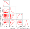 |
Fig. 1. Distribution of physical properties of galaxies drawn from the PROSPECTOR-β model. The redshifts and stellar masses are jointly drawn from the sum of two Schechter functions (Leja et al. 2020), the star formation rates (averaged over the last 100 Myr) are computed from the non-parametric star formation histories, while the stellar metallicities are drawn from a clipped Gaussian approximating the stellar mass-stellar metallicity relationship of Gallazzi et al. (2005). |
The PROSPECTOR-β model also provides the prescriptions for the stellar population components and their parameters that are required to generate SEDs with FSPS. For some prescriptions, PROSPECTOR-β uses the default implementation in FSPS, while for others, namely the emission from the gas component, the dust attenuation and emission, and the AGN component, it uses specific prescriptions.
The galaxy gas component is modelled as a two-component emission, the nebular continuum and the nebular emission lines. The stellar ionising continuum is self-consistently used to power nebular lines and continuum emission, following the CLOUDY code implementation within FSPS (Byler et al. 2017). The two parameters that govern the gas emission are the gas-phase metallicity log(Zgas/Z⊙) and the gas ionisation parameter log U, which is the ratio of ionising photons to the total hydrogen density. In PROSPECTOR-β, the gas-phase metallicity is decoupled from the stellar one (Shapley et al. 2015; Steidel et al. 2016), and it is drawn from a flat prior in the range −2.0 < log(Zgas/Z⊙) < 0.5, following the observations that the gas in the star forming galaxies at higher redshifts has metallicity abundances that may differ significantly from their stellar abundances (Shapley et al. 2015; Steidel et al. 2016). The ionisation parameter is instead kept fixed at log U = −2, although, as mentioned in Leja et al. (2019a), gas in star forming galaxies at higher redshift might experience a stronger ionising radiation field that requires raising the ionisation parameter to log U = −1 (Cohn et al. 2018).
The dust attenuation is modelled with two components (Charlot & Fall 2000), a birth-cloud and a diffuse dust screen. The birth cloud component adds extra attenuation towards young stars, simulating their embedding in molecular clouds and HII regions. It affects nebular emission as well. The birth cloud attenuation component scales as
and only attenuates stars that have formed in the last 10 Myr, which is the typical timescale for the disruption of a molecular cloud (Blitz & Shu 1980). In Charlot & Fall (2000) the birth cloud attenuation scales as λ−0.7, but the wavelength dependence varies across studies (e.g. Nelson et al. 2019). In PROSPECTOR-β the authors adopt a shallower dependence with wavelength, λ−1.0, which was introduced in Leja et al. (2017) to be an average value for local galaxies of different stellar masses and SFRs. The diffuse component, instead, attenuates all the light from the stars and the nebular emission of a galaxy. Its wavelength dependence is set by the Noll et al. (2009) prescription,
![$$ \begin{aligned} \hat{\tau }_{\lambda ,2} = \frac{\hat{\tau }_{2}}{4.05} [k^{\prime }(\lambda ) + D(\lambda )] \left(\frac{\lambda }{\lambda _V}\right)^n, \end{aligned} $$](/articles/aa/full_html/2024/09/aa50694-24/aa50694-24-eq5.gif)
which combines the fixed Calzetti et al. (2000) dust attenuation curve k′(λ) with a Lorentzian-like Drude profile D(λ) describing the UV dust bump, whose strength is linked to the diffuse dust attenuation index n (Noll et al. 2009; Kriek & Conroy 2013). The prescription in Noll et al. (2009) is meant to provide a robust fit to the individual galaxy SEDs and is motivated by the observations that show that a single attenuation curve, such as the Calzetti et al. (2000) curve, is insufficient to describe the diversity of attenuations found in star forming galaxies, particularly at high redshift. Therefore, a more complex law is required to describe the dust attenuation from a generic galaxy, with the Calzetti et al. (2000) law providing a reasonable basis as an average for large samples. The diffuse dust attenuation index n expresses a power-law modifier to the slope of the Calzetti et al. (2000) dust attenuation curve, allowing for dust attenuations with a flatter slope than this widely used attenuation law.
The optical depth of the diffuse dust  is drawn from a truncated (
 ,
,  ) normal distribution with mean
  and standard deviation
  , while the optical depth of the birth-cloud component
  is drawn from a truncated normal distribution of its ratio with
  , having mean
  , standard deviation
  , and range
  . The diffuse dust attenuation index n is uniformly distributed in the range −1.0 < n < 0.4.
PROSPECTOR-β includes also a prescription to model the emission of infrared radiation coming from the dust that has been heated by the starlight. This makes use of the Draine & Li (2007) dust emission templates that are based on the silicate-graphite-polycyclic aromatic hydrocarbon (PAH) model of interstellar dust (Mathis et al. 1977; Draine & Lee 1984). This model has three free parameters: Umin, representing the minimum starlight intensity to which the dust mass is exposed, γe, representing the fraction of dust mass which is exposed to this minimum starlight intensity and QPAH, describing the fraction of total dust mass in PAHs. Umin and γe have uniform priors in the ranges 0.1 < Umin < 15 and 0 < γe < 0.15, respectively, while QPAH is drawn from a truncated normal distribution having mean μQPAH = 2 and σQPAH = 2.
Accurate forward modelling of a galaxy SED requires also the addition of an AGN component. In the PROSPECTOR-β framework, this is achieved using AGN templates from the Nenkova et al. (2008a,b) CLUMPY models. These templates do not reproduce the broad and narrow-line region emission lines commonly found in quasar spectra, but they are created using radiative approximations by shining an AGN broken power-law spectrum through a clumpy dust torus medium. This model is characterised by two variables: fAGN, describing total luminosity of the AGN expressed as a fraction of the bolometric stellar luminosity, and τAGN, which is the optical depth of an individual dust clump at 5500 Å. In the PROSPECTOR-β model, a log-uniform, redshift independent prior is adopted for both parameters, specifically in the ranges −5 < log(fAGN) < log3 and log5 < log(τAGN) < log150.
For our work, we sampled 106 sets of galaxy physical and stellar population properties from the PROSPECTOR-β model prior described above and we used those to generate galaxy observed-frame SEDs with FSPS. We then integrated the SEDs in the KiDS-VIKING ugriZYJHKs bands to obtain a sample of mock apparent AB magnitudes and colours. The colours and the redshift distributions of samples selected by colour-magnitude from the PROSPECTOR-β model constitute our fiducial estimates against which the impact of the modifications of the stellar population components is evaluated. Figure 2 shows the distribution of colours resulting from the PROSPECTOR-β model.
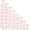 |
Fig. 2. Distribution of model colours obtained from the sample of 106 galaxies drawn from the PROSPECTOR-β model. The colours are obtained using mock apparent magnitudes in the KiDS-VIKING ugriZYJHKs bands. We display the 16th, 50th, and 84th quantile values for each colour at the top of the corresponding 1D histogram. The dotted lines in each 1D histogram are the 16th and 84th quantile values. The 2D contours enclose the 68%, 95%, and 99% of the values. |
3. Description of the stellar population components
The evaluation of the impact of the stellar population modelling components on the galaxy tomographic redshift distributions is motivated by the fact that there are still numerous phases of stellar evolution that are subject of intense research, being not well understood on both theoretical and observational grounds (see Conroy et al. 2009 for an in-depth discussion). This evaluation is carried out by modifying the stellar population components and their parameters to generate new sets of colours, and therefore redshift distributions through the colour-redshift relation, which are compared against the fiducial estimates.
We generated galaxy magnitude samples in the ugriZYJHKs bands, separately varying all the stellar population modelling components implemented in FSPS at fixed physical properties of galaxies, for a total of 21 sets of apparent magnitudes per galaxy. We also considered the case where all the modelling components are varied at the same time within the ranges set for each individual component. We labelled this augmented version as ‘P-β+’. The components we varied are: the gas emission, dust attenuation and emission, AGN component, initial mass function (IMF), velocity dispersion, specific frequency of blue straggler stars, fraction of blue horizontal branch stars, post-asymptotic giant branch phase, circumstellar asymptotic giant branch dust emission, thermally pulsating asymptotic giant branch normalisation scheme, presence of Wolf-Rayet stars, and the inter-galactic medium absorption. The new sets of magnitudes were then used to generate the galaxy colours needed to model the colour-redshift relation with the SOM (see Sect. 5).
The following sections provide a description of the physical details and the prescriptions we used to model the stellar population components we varied in our work. We also report the observationally motivated ranges over which the stellar population component parameters were varied.
3.1. Gas emission
The radiation emitted by young stellar populations ionises the surrounding gas in galaxies, producing nebular emission. The latter has two components: a nebular continuum, generated by Bremsstrahlung, recombination and two-photon emission processes, and a nebular line emission, generated by recombination and electronic transitions from forbidden and fine-structure lines. The amount of emission from the two components depends mostly on the strength of the ionising field and on the metallicity of the gas. This is why many codes rely solely on these two parameters to predict the continuum and the line emission fluxes. The FSPS code includes the nebular contribution on top of the stellar population one by means of the CLOUDY (Ferland et al. 2017) spectral synthesis code for astrophysical plasmas. The CLOUDY code measures the number of ionising photons from single stellar populations (SSPs) younger than 10 Myr, removes them from the final SED, and uses their energy to compute line luminosities and nebular continua. These are slow computations due to the complex set of equations they have to solve, therefore FSPS implements a grid of pre-computed line luminosities and nebular continua from Byler et al. (2017) that depends on SSP age, SSP and gas-phase metallicity, and ionisation parameter U.
The nebular line emission can contribute between 20% and 60% to the UV-optical rest-frame broadband fluxes and is responsible for nearly all the optical emission lines present in the spectra of star forming galaxies (Anders & Fritze-v. Alvensleben 2003; Reines et al. 2010). The higher the sSFR of the galaxy, the higher is the contribution of the emission lines to the broad-band photometry. The gas metallicity impacts the strength of the emission lines, while the ionisation parameter has an effect on the relative intensity of emission lines (Leja et al. 2017), contributing less to Balmer lines (e.g. Hα, Hβ), and more to forbidden lines (e.g. [OII], [OIII]). The nebular continuum emission contributes instead more significantly to the near-infrared fluxes (Byler et al. 2017).
The observations that the gas-phase metallicity depends on the galaxy stellar mass dates back to the early results of SDSS (Tremonti et al. 2004). Recent, higher redshift studies, have shown that the gas-phase metallicity evolves with lookback time (Bellstedt et al. 2021) and that there is a more complex dependence between gas-phase metallicity, stellar mass, and SFR (Magrini et al. 2012; Curti et al. 2020; Bellstedt et al. 2021). In PROSPECTOR-α, PROSPECTOR-β and in general SPS-based forward modelling, various prescriptions are employed to assign physically motivated values to the gas-phase metallicity and to the ionisation parameter. In Alsing et al. (2023), the metallicity of a galaxy is built up with the stellar mass production, such that the present-day value of the stellar metallicity is equal to the gas-phase metallicity. In Leja et al. (2017), the stellar and the gas-phase metallicity are also set to be equal, without allowing for the chemical evolution of the galaxy, under the assumption that the stars have the same metallicity as the gas cloud from which they had formed. Additionally, there are other studies (e.g. Leja et al. 2019a; Wang et al. 2023a) that decouple the two metallicities, with the stellar one being drawn from the Gallazzi et al. (2005) mass-metallicity relation and the gas-phase metallicity drawn from a uniform distribution of sub-solar and super-solar abundances, with ranges taken from Byler et al. (2017). The ionisation parameter is instead generally kept fixed at log U = −2, −1 (Leja et al. 2019a; Wang et al. 2023a) or related to the SFR as in Alsing et al. (2023), where the authors adopt the Kaasinen et al. (2018) relation between the gas ionisation and the SFR. Decoupling the stellar and the gas-phase metallicity and setting the ionisation parameters to a higher value are choices that are motivated by observations suggesting that the gas in high-redshift star forming galaxies experiences stronger ionising fields (Tripodi et al. 2024), possibly due to the higher cosmic SFRD (Madau & Dickinson 2014), and gas-phase metallicity abundances that differ significantly from the stellar ones (Shapley et al. 2015; Steidel et al. 2016).
To evaluate the impact of the different choices in the gas modelling on the tomographic redshift distributions, we generated three different samples of galaxies. In the first sample, which we labelled as ‘No gas emission’, we evaluated the extreme case where we turned the nebular continuum and the nebular emission lines off, such that the emission from the galaxy contains only the stellar flux, the AGN dust torus and the dust emission. The second sample, labelled as ‘Z* = Zgas’, tests the prescription of equal values of the stellar and the gas-phase metallicity against decoupling the two, without allowing for a chemical evolution in the galaxy. The third sample tests the effect of varying the ionisation parameter with respect to the fixed log U = −2 of the PROSPECTOR-β model. We labelled this sample as ‘Variable log U’. We drew the ionisation parameter for each galaxy from a uniform distribution in the range −4 ≤ log U ≤ −1, a range that is used in Byler et al. (2017) and is consistent with ionisation parameters observed in local starburst galaxies (Rigby & Rieke 2004).
3.2. Dust attenuation
Dust is a key component of the interstellar medium (ISM) of galaxies. It forms in the atmospheres of evolved stars or remnants of supernovae and gets released into the ISM (Draine 2003), where it presents itself primarily in two forms, carbonaceous dust grains, like PAHs, and silicate dust grains. Observationally, dust has two main effects: it modifies the stellar continuum, particularly in the ultraviolet to near-infrared regime, through the absorption and the scattering of starlight, and it re-emits the absorbed energy in the infrared with an SED characterised by both a continuum and various emission and absorption features.
Observations show that attenuation laws exhibit a wide range of behaviours and we might expect them to vary as function of galaxy types even among similar mass galaxies at different redshifts (see Salim & Narayanan 2020 for a recent review). Therefore, the modelling of the internal dust attenuation may dramatically impact the physical properties we derive for individual galaxies (e.g. in SED fitting, Kriek & Conroy 2013; Salim et al. 2016) since it involves not only absorption and scattering out of the line of sight, but also the complex star-dust geometry in a galaxy and the scattering back into the line of sight. Additionally, we need to provide a prescriptions for the galaxy population modelling that encompass the wide range of behaviours seen in observations.
In Sect. 2, we introduce the two-component dust attenuation model used by PROSPECTOR-β in which the radiation from all stars is subject to the attenuation by a diffuse dust component, with stars below the dispersal time of the birth cloud (10 Myr, Blitz & Shu 1980) seeing an additional source of wavelength-dependent attenuation. To evaluate the impact of different dust attenuation prescription on the tomographic redshift distribution means and scatters, we generated samples of galaxies for two additional widely-used dust attenuation laws: the Calzetti et al. (2000) and the Milky Way (MW) attenuation laws. We labelled these samples as ‘Calzetti k(λ)’ and ‘MW k(λ)’, respectively. Both of these attenuation laws are applied to all starlight equally in FSPS.
The Calzetti et al. (2000) attenuation law is controlled by a single parameter  that is related to the ratio of total to selective extinction RV = AV/E(B − V). This parameter sets the overall normalisation of the attenuation curve which has a λ−1 dependence in the 6300 Å ≤ λ ≤ 22 000 Årange and a third degree polynomial wavelength-dependence in the 1200 Å ≤ λ < 6300 Å range (stronger effect towards bluer wavelengths). We sampled
  from the same distribution as that in the PROSPECTOR-β model, meaning a truncated normal distribution with mean
  and standard deviation
  .
.
The MW attenuation law follows the prescription in Cardelli et al. (1989), which is parametrised in FSPS by means of two parameters: the first one controls the ratio of total to selective extinction RV = AV/E(B − V), while the second parameter controls the strength of the 2175 Å UV bump, a spectral feature on the interstellar extinction curve that is widely seen in the MW and nearby galaxies, but whose origin remains largely unidentified (Wang et al. 2023b). Despite being widely assumed fixed at RV = 3.1, there have been indications in the literature that the ratio of total to selective extinction deviates from this value, both in the MW itself (Cardelli et al. 1989) and in the Large Magellanic Cloud (Maíz Apellániz et al. 2017), as well as in samples of star forming galaxies from SDSS (Sextl et al. 2023). In order to conservatively select a range of values that has been measured through the observation of individual stars line of sight, we modelled the distribution of RV values using the latest results (Zhang et al. 2023) from the LAMOST survey (Zhao et al. 2012). The measurements in the MW show that the RV distribution can be modelled with a Gaussian having mean μRV = 3.25 and standard deviation σRV = 0.25. The strength of the UV bump is instead kept fixed at the Cardelli et al. (1989) determination for the MW.
3.3. Dust emission
More than 30% of the starlight energy in the Universe is re-radiated by dust at infrared and far-infrared wavelengths (Bernstein et al. 2002). When modelling the dust emission, its continuum spectrum is assumed to be close to that produced by a grey body with a single temperature (see e.g. Hensley & Draine 2021). However, the specific grain composition (typically carbonaceous PAHs and silicate grains) gives rise to different emission and absorption features due to vibrational modes, among others, in this otherwise featureless continuum (see Draine & Li 2007 for a detailed discussion).
PROSPECTOR-β, and subsequently FSPS, implements only the Draine & Li (2007) dust emission model that is parametrised by the radiation field strength and the fraction of grain mass in PAHs. Given that the dust emission starts to make a significant contribution to the galaxy flux in the mid-infrared bands, we do not expect it to have large impact on the tomographic bins selected by optical and near-infrared colours. In order to evaluate whether the dust emission has any impact on the tomographic bins via the reddest wavelength bands, we created a sample of galaxies, labelled as ‘No dust emission’, for which the extreme modelling choice is that the contribution of dust emission has been completely neglected.
3.4. Active galactic nuclei
It is known that AGNs can create a stronger emission than the regular nuclei of galaxies. This extra emission is nowadays universally accepted to be generated by the presence of a supermassive black-hole (MBH ≳ 106 M⊙) actively accreting matter. AGNs have very high luminosities (Lbol ≲ 1048 erg/s−1), strong evolution of their luminosity function with redshift (Fotopoulou et al. 2016; Kulkarni et al. 2019), and emission that covers basically the whole electromagnetic spectrum (Padovani et al. 2017). An AGN is detectable in the optical/UV due to emission from the accretion disc, mostly in the form of broad and narrow emission lines strongly ionised by the central engine, in the infrared due to thermal emission of the dust heated by the central engine, at X-ray energies due to the corona around the accretion disc, and in gamma-ray and radio due to non-thermal radiation related to the jet. For our study, the most interesting wavelength regions where the AGN emission is thought to make a contribution are the optical/UV and infrared. We expect AGN to modify galaxy colours with a degree that depends on the relative contribution of the AGN to the overall galaxy luminosity.
The AGN component implemented in FSPS comes from the CLUMPY AGN dust torus model (Nenkova et al. 2008a,b), which has proven successful in fitting the mid-infrared observations of AGN in the nearby universe (Mor et al. 2009). These templates model only the emission from the dust torus surrounding the accretion disc. However, AGN spectra in the optical/UV are also characterised by the power-law emission from the accretion disc and by the presence of broad and/or narrow emission lines coming from the strongly ionised material in the accretion disc. These lines are not modelled within the Nenkova et al. (2008a,b) templates and thus neither they are in FSPS. Furthermore, the prior values assigned to the fAGN parameter (see Sect. 2) in PROSPECTOR-β lead to a fraction of galaxies hosting AGNs (according to the criterion fAGN > 0.1, Leja et al. 2018) that is roughly 50% smaller than what the observations predict (Thorne et al. 2022a). In Leja et al. (2018), the authors point out that the fAGN parameter prior do not aim to model the fraction of galaxies hosting an AGN, but rather to fit the SEDs of galaxies hosting AGNs. Therefore, the values are motivated by the range of observed values for the power-law distribution of black hole accretion rates (Georgakakis et al. 2017). Furthermore, as pointed out in Leja et al. (2018), the range is quite uncertain due to the nonlinear correlation between the AGN bolometric luminosity and the accretion rate (Shakura & Sunyaev 1973), and the fact that the fraction of AGN bolometric luminosity re-processed into MIR emission by the surrounding environment is likely highly variable (Urry & Padovani 1995). A more informative prior range based on the comparison between the AGN and the galaxy luminosity function is therefore desirable, possibly based on what observations on large samples of galaxies predict (Thorne et al. 2022a).
To evaluate the impact of AGN models on the colour-redshift relation, we generated four different samples of galaxies. In one, we modified the PROSPECTOR-β prior by setting the AGN luminosity fraction to zero fAGN = 0, such that no AGN emission is present. We labelled this sample as ‘No AGN’. In the other three samples, we substituted the Nenkova et al. (2008a,b) templates with the parametric quasar SED model presented in Temple et al. (2021). This model has been calibrated using the observed ugrizYJHKW12 colours of the SDSS DR16 quasar population (Lyke et al. 2020) and is aimed at covering the full AGN contribution in the 912 Å ≤ λ ≤ 30 000 Å rest-frame wavelength range. It models the blue continuum in the 900 Å ≤ λ ≤ 10 000 Å range due to the low-frequency tail of the direct emission from the accretion disc, the emission from the hot dust torus in the 10 000 Å ≤ λ ≤ 30 000 Å range, the Balmer continuum at ∼3000 Å, the broad and narrow emission lines in the optical/UV region, and the Lyman-absorption suppression, which has the effect of setting the model flux to zero at all wavelengths below the Lyman limit at λLLS = 912 Å.
In swapping the Nenkova et al. (2008a,b) templates with the Temple et al. (2021) ones, the only parameter of the PROSPECTOR-β model we needed is fAGN, the total luminosity of the AGN expressed as a fraction of the bolometric stellar luminosity. We computed the bolometric luminosity for the AGN component as Lbol, AGN = fAGNLbol, galaxy and we followed the prescription in the Temple et al. (2021) templates code repository1 to relate the AGN bolometric luminosity to the monochromatic 3000 Å continuum luminosity and to the absolute i-band magnitude at z = 2, as defined by Richards et al. (2006), two quantities that are necessary to the code to produce the AGN spectrum with the right units and normalisation. We generated three samples of galaxies with the Temple et al. (2021) templates. The first one, labelled as ‘Temple+21 QSO’, uses the Baldwin effect (Baldwin 1977) to control the balance between strong, peaky, systemic emission and weak, highly skewed emission of the high-ionisation UV lines as function of redshift. In the second sample, labelled as ‘Temple+21 QSO RELB’, the balance is randomly drawn to allow for more diversity in the population of galaxies2. In the third sample, we only used the narrow emission line templates to reproduce the population of galaxies hosting AGNs where the dust torus blocks the view to the broad-line region. We labelled this latest sample as ‘Temple+21 Nlr’. The motivation in using the Temple et al. (2021) templates resides in a better agreement of the latter with observed AGN colours with respect to the use of the Nenkova et al. (2008a,b) templates (see Appendix A), which is due to the latter containing only the contribution from the dust torus emission.
3.5. Initial mass function
The stellar IMF describes the distribution of birth masses of stars and it influences most observable properties of stellar populations and thus galaxies. The first observational characterisation of the IMF for stars in the Milky-Way is that of Salpeter (1955), who finds that the IMF can be described as a power-law of the stellar mass with slope Γ = −2.35 for M* ≥ 0.5. More modern IMFs have been described in the works of Kroupa (2001) and Chabrier (2003), where the IMF power-law has the same slope than the Salpeter (1955) one at high stellar masses, but fewer low-mass stars. These three IMFs are the most commonly used ones in extra-galactic studies and are generally referred to as MW-like IMFs. One of the key assumptions in modelling them has been their universality, such that galaxies in the close and far Universe were assumed to have the same IMF also found in the Milky Way, meaning that they do not depend on redshift, morphological type, local metallicity, star formation rate, or any other parameter. However, observations conducted in the last decade using spectroscopic, dynamical, and gravitational lensing measurements have instead shown the existence of a variety of IMFs. Massive ETGs, for instance, show deviations from the Milky Way in the form of more bottom-heavy IMFs (i.e. excess of low-mass stars, Smith 2020; Parikh et al. 2024). Other recent studies support instead the existence of more top-heavy (i.e. more high mass stars produced) IMFs in nebular dominated galaxies in the early Universe (Cameron et al. 2023), as predicted by theoretical works (Chon et al. 2021; Sneppen et al. 2022).
In SPS, the IMF determines the relative weights that are assigned to the different parts of the isochrones. This implies that if a broad-band colour is dominated by a single phase of stellar evolution, then the IMF has little to not impact to it. However, if a broad-band colour is determined by a mixture of different evolutionary phases, then the IMF will down-weight or up-weight a specific phase, leading to IMF-sensitive changes in the broad-band colours. Typical colour changes induced by the IMF are of the order of 0.1 mag in the near-IR at intermediate ages (see Fig. 7 in Conroy et al. 2009). In addition to colours, the rate of luminosity evolution of a galaxy is also sensitive to IMF, being strongly related to the logarithmic slope of the IMF (see Fig. 8 in Conroy et al. 2009). Therefore, different IMFs can induce different predicted colours and mass-to-light ratios, which, in turn, lead to different predictions for physical properties of galaxies if a wrong IMF is assumed in the analysis.
PROSPECTOR-β models the stellar populations with a Chabrier IMF (Chabrier 2003). We therefore evaluated the impact of the IMF on the mean redshift of the tomographic bins by generating samples of galaxy properties and apparent magnitudes with two other kinds of IMF, a Salpeter (Salpeter 1955) and a Kroupa IMF (Kroupa 2001), both implemented in FSPS. We labelled these two samples as ‘Salpeter IMF’ and ‘Kroupa IMF’, respectively.
3.6. Velocity dispersion
The velocity dispersion of a galaxy, which quantifies the depth of its potential well, is not expected to make a significant contribution to broad-band colours. The observed velocity dispersion arises from the superposition of many individual stellar spectra that are Doppler shifted because of the star’s motion within the galaxy. In an integrated spectrum, such as that of a galaxy, the observed velocity dispersion is going to be similar to that of the stars dominating the light from the galaxy. This implies that for integrated spectra dominated by multiple stellar populations and kinematics (e.g. bulge and disc component), the determination of the velocity dispersion is extremely complex. Hence, many studies determine the velocity dispersion only for spheroidal systems whose spectra are dominated by the light of red giant stars.
The velocity dispersion effect is modelled in FSPS as a Gaussian broadening of the spectrum in velocity space in units of km s−1. The user provides as input the widths in terms of σ of the smoothing Gaussian. In the fiducial case, the spectra are not smoothed by this Gaussian kernel and therefore they are at the dispersion set by the theoretical or empirical stars with which the stellar templates have been produced. To allow for a variability of the stellar velocity dispersion σ* values that is physically motivated, we used the redshift-dependent stellar mass-stellar velocity dispersion relation introduced in Zahid et al. (2016):
where the redshift-dependent values of Mb, σb, α1, α2 are taken from Table 1 in Zahid et al. (2016), obtained using Sloan Digital Sky Survey and Smithsonian Hectospec Lensing Survey data at z < 0.7. The sample of galaxies generated with this prescription is labelled as ‘Variable σdisp’.
3.7. Blue horizontal branch stars
The population of horizontal branch (HB) stars consists of objects with mass similar to that of the Sun that are burning helium in their cores via the triple-alpha process and hydrogen in a shell surrounding the core via the carbon-nitrogen-oxygen cycle. These stars present a nearly constant bolometric luminosity (Sweigart 1987; Lee et al. 1990, 1994) which is largely driven by the constant mass of the Helium core when they enter this phase. A sub-population of the HB stars are the blue HB stars. They are a late stage in the evolution of low-mass stars (0.8 M⊙ ≲ M* ≲ 2.3 M⊙) found on the blue (hot) side of RR Lyrae, at the bottom of the instability strip (Culpan et al. 2021).
Observationally, blue HB stars are difficult to study for two main reasons: the paucity in the solar neighbourhood (Jimenez et al. 1998) and the characteristics of their spectra. Most blue HB stars are expected to have spectra than resemble those of main-sequence A-type and late B-type stars (Xue et al. 2008). The main differences are their stronger Balmer jump, lack of metal spectral lines (indication of low-metallicity), and stronger and deeper Balmer lines (Smith et al. 2010), which can complicate the estimation of quantities such as stellar age and metallicity (Lee et al. 2002). These features make blue HB stars similar in broad-band colours to A- and B-type stars, only distinguishable with sufficient spectral resolution and signal-to-noise.
The FSPS code includes the modelling of blue HB stars, however their contribution to the galaxy SED is turned off in PROSPECTOR-β. The blue HB stars contribution is added for stellar populations older than 5 Gyr and is parametrised by a free parameter fBHB that specifies the fraction of HB stars that are in this blue component. Following the prescription in Conroy et al. (2009), we drew this parameter for each galaxy from a uniform distribution in the range 0 < fBHB < 0.5, which we labelled as ‘Variable fBHB’. The addition of blue HB stars is expected to have a relatively stronger effect in the blue rest-frame colours rather than in the redder ones, not significantly altering the evolution of colours at late times, but rather giving rise to a constant blueward offset.
3.8. Blue stragglers
Blue stragglers are old, population II main-sequence stars extending blueward of the main-sequence turnoff point at higher luminosity, firstly identified by Sandage (1953). These objects have been found in all stellar systems, from globular (Piotto et al. 2004; Salinas et al. 2012) and open clusters (Milone & Latham 1994; Ahumada & Lapasset 1995, 2007; Rain et al. 2021) to the field population of the Milky Way (Preston & Sneden 2000; Santucci et al. 2015). They are particularly abundant in open clusters (Mathieu & Geller 2015) and they seem to violate standard stellar evolution theory in which a co-eval population of stars should lie on a clearly defined curve in the Hertzsprung-Russell diagram determined solely by the initial mass. The fact that they lie off the main-sequence is an indication of an abnormal evolution. The general consensus is that blue stragglers start as normal main-sequence stars and then undergo some form of rejuvenation via acquisition of extra mass. The probable mechanisms for the latter are mass-transfer in a close binary (McCrea 1964) or dynamically induced stellar collisions and mergers (Hills & Day 1976; Davies et al. 1994). If the first process is dominant, then blue stragglers should have a non-negligible effect on the galaxy integrated light since they might be common throughout the galaxy. Conversely, if the second process is dominant, then their effect is negligible because collisions are only important in high density environments, such as globular clusters, that contain only a small fraction of the galaxy stellar mass.
Blue stragglers cover a broader range in colours than normal main sequence stars and display A-type spectra. Li & Han (2007) found that blue stragglers makes broad-band colours bluer than ∼0.05 mag, while Xin & Deng (2005) found that they contribute up to ∼0.2 mag in the B − V colours in old open clusters. The FSPS code models the presence of blue stragglers in stellar populations older than 5 Gyr via a parameter SBS = NBS/NHB, that defines the number of blue stragglers per unit HB stars. In PROSPECTOR-β, the blue stragglers contribution to the galaxy SED is turned off. In this work, we let this parameter vary uniformly in the range 0.1 < SSB < 5.0 (Piotto et al. 2004; Conroy et al. 2009) when generating a galaxy for our sample. This range covers typical values for both globular clusters (Piotto et al. 2004) and field stars (Preston & Sneden 2000). The expectation is that they would contribute at most at the ∼0.1 mag level (Li & Han 2007; Xin & Deng 2005; Conroy et al. 2009) in the blue bands given that they are one order of magnitude less luminous than HB stars. We labelled the sample of magnitudes generated varying the fraction of blue stragglers as ‘Variable SBS’.
3.9. Asymptotic giant branch dust
Asymptotic giant branch (AGB) stars represent the last stage in the evolution of stars with masses in the range 0.1 M⊙ ≲ M* ≲ 8 M⊙. They are very luminous due to helium shell flashes, contributing up to tens of percent to the integrated light of stellar populations (Kelson & Holden 2010; Melbourne et al. 2012; Conroy 2013; Melbourne & Boyer 2013), with photospheric spectra that reflect the mixing of inner core material with the outer layers occurring during the dredge-up process. During this phase, significant mass loss occurs as stars eject their envelopes and evolve towards the white dwarf sequence. The material that surrounds the star due to the mass loss is observed to be dust-rich (Bedijn 1987). The degree of influence of this AGB dust emission on galaxy spectra is still a matter of debate (Kelson & Holden 2010; Chisari & Kelson 2012; Melbourne & Boyer 2013; Silva et al. 1998; Martini et al. 2013), but what is known is that its effect manifests mostly in the mid-infrared. Villaume et al. (2015) found in particular that dust shells around AGB stars affects galaxy spectra at λ ≳ 4 μm by a factor of ∼10 at intermediate ages ∼0.1 − 3 Gyr.
The FSPS code models the dusty circumstellar envelopes around AGB stars using the Villaume et al. (2015) model that makes use of the radiative transfer code DUSTY and of empirical prescription to assign dust shells to AGB stars in isochrones. This model is active per default in FSPS, and thus PROSPECTOR-β, and its amplitude is controlled by a free scaling parameter. We evaluated its effect on galaxy colours by generating a sample of objects for which the AGB dust model has been switched off. We labelled this sample as ‘No AGB dust model’.
3.10. Post-asymptotic giant branch stars
Post-asymptotic giant branch (post-AGB) stars are a rapid phase in the evolutionary path of 0.1 M⊙ ≲ M* ≲ 8 M⊙ stars that bridges the gap between the AGB phase and planetary nebula phase. It is one of the least understood phases because its duration ranges between 104 − 105 yr for low-mass stars, down to only few decades or centuries to the most massive objects (Pereira & Miranda 2007). After the outer layers have been removed during the mass loss of the AGB phase, post-AGB stars increases their surface temperature at almost constant luminosity, moving horizontally along the Hertzsprung-Russel diagram. At some point, the temperature becomes high enough that the post-AGB star starts ionising its circumstellar material and become observable as a planetary nebula (van Winckel 2003).
Post-AGB stars have been detected using the IRAS [12]−[25] versus [25]−[60] colour–colour diagram and the J − K versus H − K diagram (Garcia-Lario et al. 1997), because they were expected to be located in a colour region between the AGB stars and the planetary nebulae. During the transition from the tip of the AGB to the planetary nebula phase, their spectra appear as those of M-, K-, G-, F-, A- and OB-type post-AGB supergiants for a short period (van Winckel 2003), surrounded by dust shells. When the temperature increases and the dust surrounding the post-AGB stars start to diffuse, the contribution of post-AGB stars becomes important to the UV flux from a galaxy. Post-AGB stars are also the ionising source of low-ionisation nuclear emission-line regions, particularly in early-type galaxies (Belfiore et al. 2016; Byler et al. 2019).
Post-AGB stars are implemented in FSPS using the Vassiliadis & Wood (1994) tracks. The default behaviour of the code is to include these tracks as they are, but the user can freely change the weight given to the post-AGB phase. Therefore, we used this flexibility to generate a sample of galaxies where we turned off the contribution of post-AGB stars. We labelled this sample as ‘No Post-AGB stars’.
3.11. Thermally pulsating asymptotic giant branch stars
Thermally pulsating AGB stars (TP-AGB) represent short-living phases of the AGB which, together with AGB, HB and blue straggler stars, are important phases for SPS modelling due to their high bolometric luminosities compared to main sequence stars. TP-AGB arise from the instability that AGB stars undergo during the helium shell burning. When the latter receives new helium produced by the outer hydrogen shell fusion, the helium shell is not immediately able to adjust to the increased energy output, leading to a thermal runaway. This instability is typical of stellar populations older than 108 yr, hence having initial masses ≲5 M⊙. Therefore, TP-AGB stars tend to dominate the energy output redward of ∼1 μm for stellar populations that are several Gyrs old (Maraston et al. 2006). Their contribution has been debated for decades, but recently Lu et al. (2024) reported the detection of TP-AGB star signatures in the rest-frame near-infrared spectra of three young massive quiescent galaxies at z = 1 − 2.
TP-AGB stars are included in FSPS and their contribution can be altered using a weight factor. The default set of FSPS parameters uses the Villaume et al. (2015) TP-AGB normalisation scheme. However, FSPS allows for other two normalisation schemes to be used, the default PADOVA (Girardi et al. 2000; Marigo & Girardi 2007; Marigo et al. 2008) isochrones and the Conroy & Gunn (2010) normalisation, which we used to generate two additional galaxy samples labelled as ‘TP-AGB Padova 2007’ and ‘TP-AGB C&G 2010’, respectively. The Conroy & Gunn (2010) normalisation effect can be further controlled by shifting the bolometric luminosity log Lbol and the effective temperature log Teff of the TP-AGB isochrones with respect to the calibrated values presented in Conroy & Gunn (2010). The hotter the TP-AGB star, the bluer is the emission compared to its cooler sibling. Therefore, shifting log Lbol has primarily an effect on the bands redwards of the V-band, while shifting log Teff impacts the V − K and bluer colours. We kept these values fixed to reflect the calibration in Conroy & Gunn (2010).
3.12. Wolf-Rayet stars
Wolf-Rayet (WR) stars represent a late stage in the evolution of very massive O-type stars ≳25 M⊙, with surface temperatures ranging from 20 000 K to around 210 000 K, hotter than almost all other type of star. WR occupy the same region of the Hertzsprung-Russel diagram as the hottest bright giants and supergiants. The strong ionising radiation from these stars, coupled with the expanding outer envelope of material expelled by their strong winds, leads to Doppler-broadened recombination emission lines of helium, carbon, nitrogen, oxygen, and/or hydrogen in the WR spectrum. This outflowing material and the explosion of WR stars in supernova Ib or Ic are important components of the enrichment of the interstellar medium of star forming galaxies.
WR spectra are characterised by broad emission lines and are classified according to the ratios of emission line strengths. Though short-lived (≲107 yr), the WR stars can dominate the UV emission from young starburst galaxies, while in the UVB photometry they cannot be distinguished from normal hot stars (Crowther 2007). The FSPS code contains a spectral library to model the WR population, which is activated by default. To test its impact, we generated a sample of galaxies where the WR spectral library has been turned off and the main default library is used instead. We labelled this sample as ‘No WR’.
3.13. Intergalactic medium absorption
The bulk of baryonic cosmic matter resides in a dilute reservoir in the space between galaxies, known as intergalactic medium (IGM). The IGM has both cosmological and astrophysical implications: it can be used to test models of structure formation on the smaller comoving scales (Viel et al. 2005), its shape can bias cosmological parameter inferences from galaxy clustering (Pritchard et al. 2007), and it is the reservoir of gas from which galaxies feed. The higher the redshift of a galaxy, the more material its light has to travel through. This light is absorbed by the gaseous systems that lie along the line of sight which, at high redshift, are mostly in the form of neutral hydrogen. This effect is known as IGM absorption and at increasing redshift it can be so preponderant that all the light blueward of Lyα at 1215.67 Å becomes invisible to us.
The first modelling of the IGM absorption is detailed in Madau (1995). The author proposed a theoretical model which is able to reproduce the shape of the extinction curve as function of redshift, finding that the IGM transmission decreases with increasing redshift and that the scatter at a given redshift ranges between 20% and 70%. Later models by Meiksin (2006) and Inoue et al. (2014) updated Madau (1995) prescription for the ΛCDM model with weaker absorption at 3.5 ≲ z ≲ 5 and stronger absorption at z ≳ 6.
The FSPS code implements the IGM absorption using the Madau (1995) prescription, with a parameter that scales the IGM optical depth. The absorption impacts only the rest-frame wavelengths below the Lyα wavelength, which becomes visible in optical broad-bands, like the u-band, only from z ∼ 1.5 onwards. The default parameters of FSPS do not activate the Madau (1995) IGM absorption prescription. Therefore, we generated a sample of galaxies where we include the IGM absorption keeping the factor that scales the IGM optical depth fixed to 1. We labelled this sample as ‘Variable IGMabs’.
3.14. Combining the various prescriptions
The samples of SEDs detailed in the previous sections have been created varying one single stellar population component at a time with respect to the fiducial PROSPECTOR-β model. However, the observed population of galaxies in the Universe in reality spans all these properties ranges at the same time. Therefore, we created an additional sample of galaxies, aimed at evaluating the net effect on colours and redshift distributions of varying simultaneously all the stellar population components according to the prescriptions detailed in each subsection. We labelled this sample as ‘P-β+’.
In particular, we randomly generated galaxy SEDs using an IMF among the Chabrier, Kroupa and Salpeter ones, a dust attenuation law among the Calzetti et al. (2000), Cardelli et al. (1989) and Charlot & Fall (2000) ones, and TP-AGB stars prescription among the Villaume et al. (2015), Conroy & Gunn (2010), and PADOVA ones. We replaced the Nenkova et al. (2008a,b) templates with the Temple et al. (2021) ones obtained by modelling SDSS DR16 quasars. The Temple et al. (2021) templates are controlled by a single parameter, fAGN, which has the same meaning and values range as the one in the fiducial PROSPECTOR-β model. The gas ionisation is uniformly drawn from the Byler et al. (2017) range, while the gas metallicity is for some objects equal to the stellar metallicity and for others decoupled and uniformly drawn from the PROSPECTOR-β range. The dust emission, the AGB dust, the post-AGB stars, the WR stars and the IGM absorption are randomly turned on and off. The velocity dispersion follows the Zahid et al. (2016) prescription, while the fraction of blue HB stars and blue stragglers is uniformly drawn from the observational ranges in Conroy et al. (2009).
Figure 3 shows, for an exemplary galaxy, the directions in colour-magnitude space towards which a galaxy can move when we vary one stellar population component at the time. The fiducial r-band magnitude and g − r colour are represented as a black point, while the arrows point towards the set of magnitudes and colours generated with a different stellar population component. The P-β+ component (magenta arrow) represents the net movement in colour-magnitude space due to all the varied components.
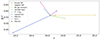 |
Fig. 3. Exemplary illustration of the directions in which a galaxy can move in colour-magnitude space when we vary a single stellar population component at a time with respect to the fiducial case (black point). We only show some of the variants that induce the most significant changes in the g − r vs. r colour-magnitude plane. |
4. Impact of stellar population components on galaxy colours
In this section, we evaluated the impact that the different stellar population components have on both the rest-frame and the observed-frame galaxy colours. For each of the 106 galaxies, we computed the difference between the rest-frame and the observed-frame colours estimated with the fiducial PROSPECTOR-β model and those estimated varying each stellar population model component, Δ(colour) = colourfiducial − colourcomponent. We compute this difference for the u − g, g − r, r − i, i − Z, Z − Y, Y − J, J − H and H − Ks colours. We selected galaxies having observed-frame i ≤ 25.3 to reproduce the Rubin-LSST Y10 lens gold sample cut (Mandelbaum et al. 2018). The use of the rest-frame colours allows us to understand the impact of the individual spectral features on the broad-band integration of galaxy spectra, while the observed-frame colours have the aim of reproducing the colour variation that we would observe in a survey that has a similar photometric precision as that expected from Rubin-LSST. The convolution of the colour difference with the redshift distribution of our sample of galaxies has the effect of smearing the colour difference across the wavelength space. The cut is applied on the i-band magnitude in the fiducial sample and this selection of galaxies is then held fixed for all variants. This ensures that we evaluated the colour differences on a per-galaxy basis.
4.1. Impact on an example galaxy SED
Figure 4 shows the comparison between FSPS generated observed-frame spectra for a subset of the different choices on the stellar population components presented in Sect. 3. The spectra belong to the same galaxy at z = 0.04. Different choices have a dramatic impact on the spectral appearance of the galaxy which, in turn, reflect on the galaxy magnitudes and colours. In this figure, we compare the effects of varying the IMF (red curve), the attenuation law (green curve), the AGN prescription (magenta curve) and the presence of gas emission (blue curve) with respect to the fiducial PROSPECTOR-β model (black curve), leaving all other parameters fixed. The Salpeter IMF produces a galaxy spectrum that overall is fainter with respect to the fiducial case that uses a Chabrier IMF. This leads to fainter magnitudes that might impact the detection of the galaxy in a flux-limited survey, and hence may impact the mix of physical properties of galaxies detected at a given colour. Changing the attenuation law from the fiducial prescription in PROSPECTOR-β to the Calzetti et al. (2000) model instead induces a wavelength-dependent modification of the galaxy spectrum. The latter is particularly evident towards bluer wavelengths, where the effect of the attenuation is more prominent. Changing the AGN prescription to the one of Temple et al. (2021), instead, gives rise to an overall brighter spectrum due to the continuum increase, but most notably leads to the appearance of the characteristic broad-line emission of AGN (see e.g. the [NII] and Hα complex in the light yellow bar). Removing completely the modelling of the galaxy gas emission leads to an overall decrease in flux due to the lack of nebular continuum and the disappearance of the emission lines that reveal the underlying absorption lines of the stellar component. The galaxy chosen as an example has a high value of the fAGN parameter to emphasise the dramatic effect of changing the AGN prescription. The units are not arbitrarily rescaled, in order to highlight the effect of varying the stellar population components at fixed physical properties on the galaxy’s flux.
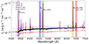 |
Fig. 4. Five different modelled observed-frame galaxy spectra belonging to intrinsically the same galaxy at z = 0.04. The black line refers to the spectrum generated with the fiducial PROSPECTOR-β model parameters, while the red, green, magenta and blue curves show the spectra generated varying the IMF (‘Salpeter IMF’), the attenuation law (‘Calzetti k(λ)’), the AGN prescription (‘Temple+21 QSO’) and removing the gas component (‘No gas emission’), keeping the other model parameters fixed. The vertical bands mark the regions where some of the most prominent emission lines appear. The emission line names are reported in black. The spectra units are not arbitrarily rescaled to highlight the effect of varying the stellar population components at fixed physical properties of galaxies on the continuum flux. |
4.2. Impact on rest-frame galaxy colours
Figure 5 shows the distribution of the rest-frame colour differences for all the SED modelling components. We report in the figure the median photometric errors of the COSMOS2020 sample (Weaver et al. 2022) that has a similar photometric precision to that expected by Rubin-LSST (see Appendix C). The distributions are plotted using a box plot representation to capture the relevant quantile ranges of the distribution of colour differences. The wider the distribution and the more offset its median with respect to the fiducial value, the larger is the effect on colours of the SED model component we vary. For the rest-frame case, the SED components that seem to have an appreciable impact on the colour distributions are those related to the dust attenuation, the AGN prescription, the gas physics and, consequently, the combined P-β+ sample.
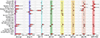 |
Fig. 5. Rest-frame colour differences between the fiducial galaxy sample (PROSPECTOR-β) and those obtained modifying one stellar population component at the time (y-axis labels). The coloured widths are the sum in quadrature of COSMOS median photometric errors in the two respective bands to indicate distinguishability on a single galaxy basis. The vertical black bars and the white dots on top of them represent the median values of each rest-frame colour difference. The light red boxes show the interquartile range (75th–25th percentile), while the whiskers represent the 84th–16th percentile ranges. |
Changing the dust attenuation prescription from the PROSPECTOR-β fiducial two components Charlot & Fall (2000) to the Calzetti et al. (2000) (‘Calzetti k(λ)’ label) or Cardelli et al. (1989) (‘MW k(λ)’ label) ones induces a wavelength-dependent change in the rest-frame colours, especially in the bluer bands, where the effect of the dust attenuation is more prominent. The distributions of colour differences for the Calzetti et al. (2000) attenuation law are moved towards bluer colours than the fiducial case. The median value of the distributions is beyond the median COSMOS2020 errors for all the optical colours, while it is within the errors for the near-infrared ones. The 84th–16th percentile values also follow the same trend. For the Cardelli et al. (1989) MW dust attenuation prescription, we have a similar, but mitigated behaviour. The median value of the distributions are outside the median COSMOS errors for the u − g and the g − r colours, while they are within the errors for the other redder colours. Interestingly, the i − z rest-frame colour distribution is biased towards redder colours than the fiducial model. The 84th–16th percentile values are instead wider than the errors only for the u − g and the g − r colours, and only marginally for the i − z rest-frame colour.
The AGN prescription effect differs depending on whether we completely remove the AGN component or on whether we use the Temple et al. (2021) model. Removing the AGN component (‘No AGN’ label) has an appreciable effect only in the rest-frame J − H and H − Ks bands since the AGN prescription in FSPS aims at reproducing the dust torus emission that is stronger in the infrared bands. Replacing the FSPS AGN model with the Temple et al. (2021) model (‘Temple+21 QSO’ and ‘Temple+21 QSO RELB’ labels) leads to noteworthy changes in the rest-frame near-UV/optical colours and in the J − H and H − Ks colours. The colour difference in the near-UV/optical is mainly due to the fact that the Temple et al. (2021) prescription aims at modelling also the emission coming from the gas in the broad-line region that is subject to the intense ionising radiation field of the accretion disc. The difference in the J − H and H − Ks colours is instead due to a different treatment of the dust torus emission that leads to the Temple et al. (2021) model producing slightly redder colours than the fiducial PROSPECTOR-β model. By modelling the emission from the ionised gas in the narrow-line region only (‘Temple+21 Nlr’ label), the rest-frame optical colour differences are mostly within the median COSMOS2020 photometric errors, while the different prescription becomes detectable in the J − H and H − Ks colours. This is due to the lack of dust torus emission when modelling the narrow-line region only, which predicts bluer colours with respect to the FSPS AGN prescription.
The different gas physics prescriptions induce changes in the intensity or presence of emission lines which in turn reflect on the galaxy rest-frame colours. Removing completely the modelling of emission lines (‘No gas emission’ label) results in colour differences that are larger than the median photometric errors for the u − g, g − r and r − i optical colours. In particular, the u − g and g − r distributions are biased towards bluer colours, while the r − i towards redder colours. The disagreement with the fiducial model is particularly prominent for the r − i rest-frame colour, because this is the wavelength range where the Hα, [NII], and [SII] lines fall. The effects in the u − g and g − r colours are instead mainly driven by the complete absence in modelling the [OII], Hβ and [OIII] lines. Changing the ionisation state of the gas results in a variable relative intensity of the emission lines, which is particularly evident for the ([OIII]λλ4959, 5007 Å/[OII]λλ3726, 3729 Å) and the ([OIII]λ5007 Å/Hβ) emission line ratios. These ratios fall into the u and g bands as testified by the 84th–16th percentile distribution values in the u − g and g − r rest-frame colours being outside of the median photometric errors and leading to bluer and redder colours, respectively, if compared to the fiducial model. The use of a different prescription to assign the gas-phase metallicity to galaxies leads in a change of the overall intensity of the nebular continuum, as well as the intensity and presence of certain complexes of emission lines. The u − g and g − r colours are the ones most affected by the change in the gas prescription, with distributions that are biased in the opposite sense with respect to the ‘Variable log U’ case. Besides the lines already mentioned falling into these bands, a visual inspection of the rest-frame spectra shows that other lines contribute to the variation in rest-frame colours, for instance the presence or absence of the [OIII]λ4363 Å line.
The distribution in the rest-frame colours for the P-β+ case can be considered as an average of the effects of all the variable SED components that we implement when creating this sample of galaxies. The optical colours are dominated by the combined effect of the dust attenuation law and AGN prescription that bias the P-β+ colours towards bluer ones than the fiducial model. The Z − Y, Y − J and J − H colour distributions are within the median photometric erros, while the H − Ks infrared colour is biased towards bluer colours being an interplay between the Temple et al. (2021) prescription for the dust torus emission and the lack of dust torus prescription in the narrow-line AGN modelling when compared to the fiducial model.
4.3. Impact on observed-frame galaxy colours
Figure 6 shows the same set of SED modelling components and colour differences, but in the observed-frame, thus mimicking the effects we would observe in a survey that has a similar photometric precision than that expected from Rubin-LSST. The figure shows that the AGN prescription and the dust attenuation law are the main drivers of the change in observed-frame colours also in this case. Their impact leads to a large fraction of galaxies showing colour variations that exceeds the median photometric errors, implying detectability on a single galaxy basis. Furthermore, the redshift leads to dilution of the colour differences across the wavelength space. This leads, on one hand, to the mitigation of the effects of some of the components, for instance the prescription for the gas ionisation and the gas metallicity that have now most of the galaxies within the photometric errors, while on the other hand, a wider distribution of colour difference values for the AGN prescriptions and dust attenuation laws. The P-β+ observed-frame colours follow the trends of the main drivers of the colour changes, namely the dust attenuation and the AGN prescription. In particular, all the distributions are biased towards bluer colours with respect to the fiducial case.
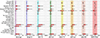 |
Fig. 6. Observed-frame colour differences between the fiducial galaxy sample (PROSPECTOR-β) and the ones obtained by modifying one stellar population component at a time. The coloured widths are the sum in quadrature of COSMOS median photometric errors in the two respective bands to indicate distinguishability on a single galaxy basis. The vertical black bars and white dots on top of them represent the median values of each observed-frame colour difference. The light red boxes show the interquartile ranges (75th–25th percentiles), while the whiskers represent the 84th–16th percentile ranges. |
Concerning the dust attenuation, the distribution of colour differences for the Calzetti et al. (2000) attenuation law is moved towards bluer colours than the fiducial case. The median value of the distributions is beyond the median photometric errors for all the optical colours, while it is within the errors for the near-infrared ones. The 84th–16th percentile values are instead all beyond the errors except for the H − Ks colour. For the Cardelli et al. (1989) MW dust attenuation prescription, we have a similar, but mitigated behaviour. The median value of the distributions are outside the median COSMOS2020 errors for the u − g and the g − r colours, while they are within the errors for the other redder colours. The 84th–16th percentile values are instead wider than the errors only up to the Z − Y colour.
Removing the AGN modelling does not lead to changes in the observed colours that are beyond the photometric errors, while replacing the FSPS AGN model with the Temple et al. (2021) model leads to noteworthy changes in the observed-frame colours from the u − g down to the Y − J colour. In this case, the median of the colour difference distributions is only marginally offset from zero, but the 84th–16th percentile distributions are heavily biased towards bluer colours. By modelling the emission from the ionised gas in the narrow-line region only, the observed-frame colour differences are within the photometric errors. Therefore they contribute only marginally to the colour variation with respect to the fiducial model. The other SED modelling choices contribute little to the colour variation, with the case of the modelling of the TP-AGB phase that does not impact at all the studied bands. Therefore, we will not further discuss these two modelling components in the rest of this work.
Figure 6 is interesting because it provides us with a quantitative estimate of how much the colours of a population of galaxies change when we vary the SED modelling components, thus guiding the evaluation of which SED components can be left at the fiducial values and which instead require more careful modelling and constraints from the observations. In turn, this is tightly linked to the fact that not accurately knowing the colour distributions makes the modelling of the colour-redshift relation highly uncertain. Indeed, even if the effect of varying the SED component cannot be detected on a colour for a single galaxy when using median COSMOS photometric errors, it could however be of significance on the ensemble colour distribution of a survey and thus on its redshift distributions.
5. Impact of SED modelling on the SOM-based colour-redshift relation
In this work, we modelled the colour-redshift relation using the Masters et al. (2015, 2017) SOM, which maps the empirical distribution of galaxies in the multi-dimensional colour space spanned by the COSMOS u band imaging from CFHT, the griz imaging from Subaru Suprime Cam, and the YJH imaging from the UltraVista survey (McCracken et al. 2012). In its original implementation, the SOM was trained on the COSMOS 2015 (Laigle et al. 2016) ugrizYJHKs photometry. We used the KiDS-VIKING ugriZYJHKs remapped version (McCullough et al. 2024) of the Masters et al. (2015, 2017) SOM. In the previous section, we have assessed the dramatic impact that the different stellar population modelling choices have on colours. We show in this section that this directly affects the colour-redshift relation as modelled by the SOM, by evaluating the impact that different stellar population modelling choices have on a galaxy SOM cell assignment and on the mean redshift estimation per SOM cell.
For each galaxy belonging to the different samples that we built by varying the stellar population components, we performed the SOM cell assignment procedure using the observed-frame model colours, without adding photometric noise and assuming equally sized errors in all colours, which is equivalent to a perfect cell assignment. We show in Appendix B that the use of COSMOS2020 photometric errors has an impact on the SOM cell assignment of a galaxy that is negligible compared to its variation in colours due to stellar population choices.
Table 1 shows the fraction of galaxies whose assigned cell in the SOM change with respect to the one assigned with the fiducial model. The left-hand column shows the fraction when considering the full sample of 106 galaxies, while the right-hand column shows the case of galaxies belonging to the Rubin-LSST Y10 sample, i ≤ 25.3. We applied the Y10 cut based on the i-band magnitudes of the fiducial sample in order to always compare the same set of galaxies. The Y10 cut selects 191 025 galaxies. The fractions track the variation in the colour distribution reported in Sect. 4, with the largest fraction of cell change in the full sample arises from the attenuation laws. Indeed, the Calzetti et al. (2000) and Cardelli et al. (1989) attenuation laws lead to a change of 89.6% and 88.6%, respectively, in the assigned cells with respect to the fiducial case for the full sample, while for the Y10 cut the values drop to 80.9% and 76.3%. The AGN prescription also leads to a SOM cell assignment variation, which is less dramatic than the attenuation law case, but still leading to a fraction of cell assignment change of roughly 57% (∼43%) variation in the full sample (Y10 sample) when adopting the Temple et al. (2021) AGN templates. The fractions are instead lower (∼11%) when using only the narrow-line region template. The P-β+ case leads instead to a fraction of cell change of 84.2% for the full sample and 82.2% for the Y10 sample. Another SED component that generates a sensible change in the SOM cell assignment is that provided by the removal of the gas component emission, ‘No gas emission’. Although the effect on the galaxy colours distribution of this component is smaller than other components, such as AGN prescription and dust attenuation laws, the colour change they lead to causes a variation in the SOM cell assignment with respect to the fiducial case of 43.6% for the full sample and 63.1% for the Y10 sample. This is due to the unrealistic galaxy population that this case models, which is consistent with real galaxies only in the case of quiescent objects. It is also interesting to note that the variation in the SOM cell assignment is greater for the Y10 sample than for the full sample. The reason resides in the i-band cut preferentially selecting star forming objects. In the full sample there are passive galaxies of which the ‘No gas emission’ actually constitute a good representation of their SEDs, but in the Y10 sample most of them are not included in the magnitude cut. Therefore in this latter case we are comparing galaxies with no gas emission against mostly star forming objects who could not be properly model in colours unless gas is added to their SEDs, hence the larger fractional change.
Fraction of galaxies changing SOM cell assignment as function of the SED component.
Other stellar population components that give a large (≳10%) SOM assignment change are the ‘Salpeter IMF’ (14.9% for the full sample and 23.4% for the Y10 sample), the ‘Variable log U’ (17.2% for the full sample and 25.0% for the Y10 sample), the ‘Z* = Zgas’ (17.2% for the full sample and 25.0% for the Y10 sample), and the ‘No WR’ (11.3% for the full sample and 12.2% for the Y10 sample) components, with the latter inducing a change due to its impact on the rest-frame u-band magnitudes. The other stellar population components lead to variations which are ≲10%.
Having assigned each galaxy to a SOM cell, we aim at characterising how much the occupation number and the mean redshift of each cell change with respect to the fiducial case when using samples generated with different stellar population components. The left-hand panel of Fig. 7 shows the distribution of the relative difference in the occupation numbers of the SOM cells. For each pair of fiducial and variable component model, we consider only the cells that are populated by both galaxy samples. We report the relative difference as (Nj, comp−Nj, fiducial)/Nj, fiducial, with the light green and light blue areas in Fig. 7 showing the regions where the relative difference is within ±1% and ±10%, respectively. From this figure, we see that the only components that do not lead to a substantial variation in the cell occupation number are those related to the advanced stages of stellar evolution (blue stragglers, blue HB stars, AGB, post-AGB, TP-AGB), as well as the ‘Kroupa IMF’, ‘No dust emission’, ‘Variable σdisp’ and ‘Variable IGMabs’ components.
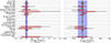 |
Fig. 7. Distributions of the relative difference in the cell occupation number (left panel) and in the cell mean redshift (right panel) with respect to the fiducial case. For each pair of fiducial and variable component model, we consider only the cells that are populated by both galaxy samples. The relative differences in the cell occupation number are shown as (Nj, comp − Nj, fiducial)/Nj, fiducial for clarity. The black vertical bars and the white dots on top of them represent the median value of (Nj, comp − Nj, fiducial)/Nj, fiducial, the boxes represent the 75th–25th percentile ranges and the whiskers represent the 84th–16th percentile ranges. The light green and light blue areas show the regions where the relative difference is within −0.1 ≤ (Nj, comp − Nj, fiducial)/Nj, fiducial ≤ 0.1 and −0.01 ≤ (Nj, comp − Nj, fiducial)/Nj, fiducial ≤ 0.01, respectively. The right panel shows the distributions of the differences in the mean redshift per cell between the fiducial case and the SED components variation cases normalised by 1 + z. The elements on the plot have the same meaning, but the light green and light blue areas show instead the regions where the relative difference of cell mean redshift is within |


The right-hand panel of Fig. 7 shows instead how the mean of the redshift distribution in each cell change when one varies the stellar population components with which galaxy spectra are built. In particular, we report the difference in the mean redshift between the fiducial model and those obtained by varying one stellar population component at the time normalised by 1 + z,  . The light green and light blue areas in Fig. 7 show the regions where the relative difference is within ±0.1% and ±1%, respectively. The same components that have percent level variation in the occupation number are those that have permille level variation in the mean redshift of the SOM cells, while the other components induce relative variations in the mean redshift that are in some cases even greater than the percent level.
The results shown in Fig. 7 highlight the direct impact that varying a single stellar population component has on the colour-redshift relation. For the same galaxy, varying the spectrum generates a variation in colours which in turn associates the galaxy to a different SOM cell. The combined effect of the population of galaxies results in a change of cell occupation numbers and mean redshift per cell that at the cell level is much greater than the percent and permille nominal precision requirements by Stage III and IV surveys, respectively.
6. SED modelling impact on the redshift distribution means and scatters
In this section we evaluated the impact of varying the SED modelling components on the redshift distribution of our sample of simulated galaxies. First, we evaluated how the entire redshift distribution of the sample of galaxies changes between SED model variants when we apply a pure magnitude selection. Then, we used these magnitude-selected samples to create tomographic bins following the prescription in McCullough et al. (2024). This procedure allows us to evaluate the impact on the mean and the scatter of the tomographic redshift bins induced by the variation in the SED modelling components.
In forward modelling the galaxy population, any mis-specification of the SED model would result in a partial compensation of this impact by the fitted distribution of physical properties of galaxies, particularly the stellar mass function (SMF). What effect this has in practice depends on the galaxy data being used as a constraint and on the degrees of freedom that are given to the galaxy population model. We introduced three limiting cases, which we used to try to evaluate the extent to which this may compensate for the impact of SED mis-modelling on the colour-redshift relation. We assume that only the SMF that is being fitted is used to compensate for the SED mis-modelling, while other physical properties such as metallicity and star formation history are kept as-is. The SMF is indeed the most flexible element of the galaxy population model for fitting the observed abundance of galaxies, which is the primary constraint in the forward-modelling of photometric surveys. Degrees of freedom on other galaxy physical property distributions may also have an interplay with SED modelling, which however is beyond the scope of this work to investigate. The three SMF cases we consider are:
-
‘Fixed SMF’: the different variants keep the distribution of all physical properties of galaxies fixed and we apply the i-band selection separately on each variant. This leads to different galaxies, and different total numbers of galaxies, to be selected in each variant.
-
‘Fitted SMF’: we apply an overall multiplicative correction of stellar mass that compensates the SED modelling choice dependent stellar mass-to-light ratio. This is done in such a way that the overall abundance of our apparent i-band magnitude limited sample is kept fixed.
-
‘Fitted SMF of (type, z)’: we assume a highly flexible fit of the SMF as a function of galaxy type and redshift. We realise this practically such that the exact same set of galaxies is selected into the magnitude limited sample, regardless of which variant of the SED modelling is being considered.
6.1. The impact on the magnitude-limited sample
A magnitude-limited selection of target galaxies is generally performed using a sharp cut in colours or magnitudes. Since the results presented in Sect. 4 highlight the dramatic effect that varying the SED components has on the galaxy magnitudes and colours, we expect a similar effect to be reflected on the redshift distributions resulting from a magnitude-limited selection. In the case of a Stage IV galaxy survey like Rubin-LSST, the LSST DESC requirements (Mandelbaum et al. 2018) for the weak lensing and galaxy clustering analysis on the systematic uncertainty in the mean and redshift scatter of each source tomographic bin refer to a sample of galaxies, the Y10 lens gold sample, that has a limiting magnitude of ilim = 25.3. We used this value to select magnitude-limited samples of objects from each of the 22 sets of galaxies generated by varying the SED modelling components.
We computed the mean  and the standard deviation σz, comp for each of the 22 resulting magnitude-limited redshift distributions N(z)comp and compared those against the mean
  and the standard deviation σz, fiducial obtained for the magnitude-limited fiducial sample N(z)fiducial,
The errors on these estimates are obtained using bootstrap resampling. The procedure involves repeatedly sampling with replacement from the original set of galaxies to create multiple bootstrap samples, applying the magnitude selection, computing the mean for each bootstrap sample and then the standard deviation of these bootstrap means. We generated a total of 103 bootstrap samples.
For the ‘Fixed SMF’ sample, the variation in the stellar population components generates samples of galaxies that contain a different number of objects brighter than the i-band magnitude cut. The number of galaxies at i ≤ 25.3 ranges from 148 447 galaxies in the case of the ‘Salpeter IMF’ to 243 329 galaxies in the case of ‘Temple+21 QSO’. However, in modelling a galaxy population, an important property that is fitted to the observations is the total number of galaxies that the model produces. To account for this, the ‘Fitted SMF’ sample matches the dn/dmi of each of the 22 components to the fiducial one by applying a constant magnitude shift to the i-band. This corresponds to an overall multiplicative correction of stellar mass that compensates the SED modelling choice dependent stellar mass-to-light ratio. We estimated the i-band magnitude shift for each component variant such that the total number of galaxies having i ≤ 25.3 is equal to that of the fiducial sample (191 025). The shifted i-band magnitude distributions for the various SED modelling components are then used to select a sample and compute the mean and the standard deviation of the magnitude-limited redshift distributions. We computed the errors on these estimates as in the previous case (i.e. via bootstrap resampling).
Figure 8 shows the differences  and Δ(σz)comp between the mean (left-hand panel) and the scatter (right-hand panel) of the magnitude-limited fiducial redshift distributions and those obtained for each varied SED modelling component. The light blue stars refer to the dn/dmi matched case (‘Fitted SMF’), while the orange circles to the unmatched case where the i-band selection produces samples of different numbers of galaxies (‘Fixed SMF’). The light blue and orange error bars in the black boxes in the bottom right corners show the bootstrap-estimated errors on the mean and the scatter of each
  and Δ(σz)comp. In particular, we report the error averaged across all the evaluated components. The blue and the red bars show the systematic uncertainty requirements on the redshift distribution mean and scatter for the galaxy clustering and weak lensing 3 × 2 pt analysis of Rubin-LSST Y10, as detailed in Mandelbaum et al. (2018). The requirements state that the systematic uncertainty in the mean redshift of each tomographic bin should not exceed 0.001(1 + z) for the weak lensing 3 × 2 pt analysis and 0.003(1 + z) for the galaxy clustering analysis, while the systematic uncertainty in the photometric redshift scatter should not exceed 0.003(1 + z) for the weak lensing 3 × 2 pt analysis and 0.03(1 + z) for the galaxy clustering analysis.
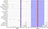 |
Fig. 8. Differences |


The ‘Fixed SMF’ case (orange circles) shows the dramatic impact that a sharp magnitude cut has on the mean and standard deviation of the magnitude-selected galaxy redshift distributions. We find that a magnitude selection leads to changes in the mean of the redshift distributions up to Δz ∼ 0.1. The ‘Kroupa IMF’, ‘Salpeter IMF’, and ‘No gas emission’ samples lead to redshift distributions that are biased low with respect to the fiducial case, since they tend to shift the dn/dmi towards fainter galaxies that are not included in the magnitude cut. Keeping the SMF constant while changing the latter modelling components will inevitably lead to a loss of galaxies with fainter i-band magnitudes compared to the fiducial case, as it is visible from the behaviour in Figs. 4, 5 and 6. On the other hand, the ‘Temple+21 QSO’, ‘Temple+21 QSO RELB’, ‘Calzetti k(λ)’, ‘MW k(λ)’, and ‘P-β+’ samples tend to shift the dn/dmi towards brighter galaxies than the fiducial case, leading to redshift distributions that are biased high.
The mentioned components bias the mean of the redshift distribution with respect to the fiducial case by an amount that exceeds the requirements for the Y10 weak lensing and galaxy clustering analysis. The other components instead cause biases that are within the Y10 requirements. In the case of the redshift scatter, all biases are always within the requirements for the galaxy clustering Y10 analysis, while for the weak lensing analysis the components mentioned above bias the redshift scatter by an amount that is beyond the Y10 requirements.
Matching the total number of galaxies to that of the fiducial case only partially mitigates the bias on the mean and the scatter of the redshift distributions. In particular, the only variants that are made compatible by the matching with both the weak lensing and the galaxy clustering Y10 requirements on the redshift distribution mean are the ‘Kroupa IMF’ and ‘No gas emission’. Matching the total number of galaxies also leads the ‘Kroupa IMF’ variant to become compatible with both the weak lensing and the galaxy clustering Y10 requirements on the redshift distribution scatter.
6.2. Impact on the tomographic redshift distributions
To evaluate whether varying the stellar population modelling components introduce biases in the mean and scatter of the tomographic redshift bins, we used the galaxies assigned to the SOM cells to infer the redshift distributions for five tomographic bins built following the prescription in McCullough et al. (2024).
6.2.1. Tomographic redshift distributions construction
After selecting the magnitude-limited sample of galaxies, we performed the SOM cell assignment algorithm, such that the i-th cell ci in the SOM is populated by an associated number of galaxies, ni, with a redshift probability distribution, P(z|ci). We used the histogram of redshifts of galaxies in a cell as the model for the P(z|ci). We then sorted the cells according to their median redshift and created five equally populated tomographic bins by placing galaxies in each tomographic bin according to the median redshift of the cell they reside in. The redshift distribution of galaxies in each tomographic bin is then given by the redshift probability distribution in each cell weighted by the cell occupation,
where 𝒞i is the set of cells used in the tomographic bin. We populated the lowest redshift bin first and then we moved to the consecutive one once the total number of galaxies in each bin Ntot is roughly equal to one fifth of the full sample of magnitude-selected objects populating the SOM cells. The mean of the galaxy redshift distribution in each tomographic bin depends on the mean redshift in each colour cell  weighted by the number of galaxies per cell ni,
![$$ \begin{aligned} \bar{z}_{\mathrm{bin} }&= \frac{\int z \ N(z|\mathrm{bin} ) \ \mathrm{d} z}{N_{\mathrm{tot} }}\nonumber \\&= \frac{1}{N_{\mathrm{tot} }} \left[ n_1 \bar{z}_{c_1} + \ldots + n_{\mathcal{N} } \bar{z}_{c_{\mathcal{N} }} \right], \end{aligned} $$](/articles/aa/full_html/2024/09/aa50694-24/aa50694-24-eq33.gif)
where Ntot is the total number of galaxies in the tomographic bin. The variance of each tomographic bin is given by
where  is the redshift distribution variance per cell. In Fig. 9, we show the five tomographic bins built for the fiducial sample and for the ‘Calzetti k(λ)’ sample using the prescription highlighted above. We choose to plot this stellar population variant against the fiducial to highlight the strong impact that stellar population components might have on the tomographic redshift distributions. Indeed, the ‘Calzetti k(λ)’ is one of the components providing the largest impact on the tomographic redshift distributions. This is due to the brighter rest-frame UV emission that the ‘Calzetti k(λ)’ variant induces (see Fig. 4). This leaves the low-redshift galaxy observables unaffected, while it brightens high-redshift galaxies in the observed optical bands, hence making them more numerous in a magnitude-limited sample.
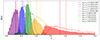 |
Fig. 9. Redshift distribution N(z) of two sets of five tomographic bins built with the prescription highlighted in Sect. 6. The filled histograms refer to the N(z)s built with the fiducial sample, while the histograms with the dashed outlines represent the N(z)s built using the ‘Calzetti k(λ)’ component. The solid and dashed vertical lines represent the mean of the tomographic bins for the fiducial and the ‘Calzetti k(λ)’ components, respectively. The legend shows the tomographic bin means and 1σ errors on the means. We use the ‘Calzetti k(λ)’ component to demonstrate our analysis methodology as it induces the largest shift in the N(z). The shift is caused by the brighter rest-frame UV emission that the ‘Calzetti k(λ)’ component induces (see Fig. 4). This leaves the low-redshift galaxy observables unaffected, while it brightens high-redshift galaxies in the observed optical bands, hence making them more numerous in a magnitude-limited sample. |
Figures 10 and 11 represent the main result of this work. Figure 10 shows the bias induced on the tomographic redshift distribution bin means when modelling the galaxy SEDs with different stellar population component choices, while Fig. 11 shows the bias induced on the tomographic bins’ scatter. The blue and red vertical bars represent the requirements for the Rubin-LSST Y10 galaxy clustering and weak lensing analysis, respectively, as detailed in Sect. 6.1. The error bars in the black boxes are obtained similarly to Sect. 6.1 (i.e. via bootstrap resampling).
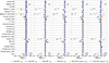 |
Fig. 10. Impact of varying the choices of the SED modelling component on the mean of the tomographic redshift distribution bins. Each panel shows a different tomographic bin, from the lowest (left-most) to the highest (right-most) redshift one. Each row represents a different SED modelling component we vary. The scatter points represent the difference between the mean redshift per bin obtained with the fiducial PROSPECTOR-β model and that obtained by varying one SED modelling component at the time. Orange scatter points are obtained by weighting the P(z|ci) for the number of simulated galaxies per SOM cell, while light blue points are obtained by weighting the P(z|ci) for the observed abundances in the Masters et al. (2015), McCullough et al. (2024) SOM cells. Circle-shaped, star-shaped and diamond-shaped scatter points refer to the cases where we perform an i-band magnitude-selection of the sample of galaxies that is different for each component, matched for the total number of galaxies and based on the fiducial i-band distribution, respectively. We report the mean errors on the difference of the tomographic bin means estimated via bootstrap resampling in the black boxes in the bottom right-hand corner of each subplot. The blue and red coloured bands refer to the Rubin-LSST Y10 galaxy clustering and weak lensing requirements, respectively. |
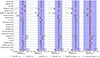 |
Fig. 11. Impact of varying the choices of the SED modelling component on the scatter of the tomographic redshift distribution bins. Each panel shows a different tomographic bin, from the lowest (left-most) to the highest (right-most) redshift one. Each row represents a different SED modelling component we vary. The scatter points represent the difference between the redshift scatter per bin obtained with the fiducial PROSPECTOR-β model and that obtained by varying one SED modelling component at the time. The orange scatter points are obtained by weighting the P(z|ci) for the number of simulated galaxies per SOM cell, while the light blue points are obtained by weighting the P(z|ci) for the observed abundances in the Masters et al. (2015), McCullough et al. (2024) SOM cells. Circle-shaped, star-shaped and diamond-shaped scatter points refer to the cases where we perform an i-band magnitude-selection of the sample of galaxies that is different for each component, matched for the total number of galaxies and based on the fiducial i-band distribution, respectively. We report the mean errors on the difference of the tomographic bin scatters estimated via bootstrap resampling in the black boxes in the bottom right-hand corner of each subplot. The blue and red coloured bands refer to the Rubin-LSST Y10 galaxy clustering and weak lensing requirements, respectively. |
The different points for a given stellar population variant represent different ways in which the redshift probability distribution in each cell is weighted towards the bin average. In particular, the orange scatter points are obtained when weighting the redshift probability distributions P(z|ci) in each cell by the number of simulated galaxies nsim that occupy that cell in the same variant. The light blue scatter points, instead, are obtained when weighting the P(z|ci) by the observed KiDS-VIKING abundance nKV in the remapped SOM (Masters et al. 2015; McCullough et al. 2024) cells, similar to what would be the case in a scheme like that of Myles et al. (2021).
At fixed variation of stellar population variant and scatter point colour, we generated three different samples of magnitude-limited objects with which we construct the tomographic bins. The circles represent the case where, for each different stellar population component, we selected the magnitude-limited sample of galaxies using the i-band magnitude distribution from that specific component (‘Fixed SMF’). This process selects different numbers of galaxies among the various stellar population components, as pointed out in Sect. 6.1. The star-shaped scatter points represent instead the case where we matched the dn/dmi of each of the 22 components to the fiducial one by applying a constant magnitude shift to the i-band magnitude distributions (‘Fitted SMF’). This process aims at matching the total number of magnitude-selected galaxies with that of the fiducial case by matching a model to the observed abundances. The diamond-shaped scatter points instead represent the case where, for each variation of the stellar population components, we selected the magnitude-limited sample of galaxies using the i-band magnitude distribution of the fiducial case (‘Fitted SMF of (type, z)’). This process effectively employs always the same population of galaxies, but with a colour-redshift relation that is established by the SOM and therefore changes for every stellar population component.
Figures 10 and 11 show that the variation of the stellar population component choices with respect to those adopted in the fiducial PROSPECTOR-β model affects the derived colour-redshift relation. This, in turn, induces biases in both the mean and the scatter of the redshift distributions of tomographic bins that are beyond the requirements set by Stage IV galaxy surveys for several of the variants. As already shown throughout the work, the components that make the greatest contribution to the bias are those related to the IMF, AGN, gas, and dust attenuation modelling, including the P-β+ component that encapsulates the net effect of all the varied SED modelling components. These variants mostly bias the redshift to higher values.
In the following sections, when presenting the biases induced by each SED modelling component, we tested the consistency with the weak lensing and clustering requirements using errors estimated via bootstrap resampling. These errors are somewhat different for every SED component however, in Figs. 10 and 11 we show only the errors averaged across all the components for plot readability.
6.2.2. Impact of the initial mass function
The first SED modelling component of which we evaluated the impact on the tomographic redshift distributions is the IMF. In our work, we tested two different widely used IMFs, the ‘Kroupa IMF’ and ‘Salpeter IMF’ that are compared against the Chabrier IMF adopted in the fiducial model. The ‘Kroupa IMF’ component (first row of Figs. 10 and 11) does not induce a dramatic shift in the mean redshift and scatter of the tomographic bins given its similarity with the Chabrier IMF. When considering the case of different magnitude-limited samples of galaxies (‘Fixed SMF’, circle-shaped points), the shift in the means induced by this component is consistent with the fiducial model within the galaxy clustering requirements in the second and third tomographic bin for nsim and in the first and third tomographic bin for nkv. It is instead consistent with the weak lensing requirements in the first, fourth and fith tomographic bin for nsim and in the fourth and fith tomographic bin for nKV. If we account for SED mis-modelling and for the observed abundances, namely, the ‘Fitted SMF’ (star-shaped points) and ‘Fitted SMF of (type, z)’ (diamond-shaped points), the ‘Kroupa IMF’ component becomes consistent with the fiducial model within the Stage IV weak lensing requirements on the mean redshift for every tomographic bin. As for the requirements on the redshift scatter, the ‘Kroupa IMF’ component is consistent with the fiducial model within the weak lensing requirements for every tomographic bin, with the only exception of the ‘Fixed SMF’ weighted by nsim case, which is consistent with the clustering requirements only in the first tomographic bin.
The ‘Salpeter IMF’ component (second row of Figs. 10 and 11) has instead a slightly different behaviour. Since we have seen in Figs. 4 and 8 that the ‘Salpeter IMF’ has a strong impact on the i-band magnitude and thus selection, this component in the ‘Fixed SMF’ case (circle-shaped points) selects a very different sample of objects with respect to the fiducial ones, thereby biasing the mean redshift of the tomographic bins well beyond the Stage IV requirements. Upon matching the total number of galaxies selected to the fiducial model (‘Fitted SMF’ and ‘Fitted SMF of (type, z)’ cases), the impact is strongly mitigated in every tomographic bin in such a way that for the highest degree of SED mis-modelling compensation (‘Fitted SMF of (type, z)’ case) we have consistency with the fiducial model within the weak lensing requirements on the redshift mean in every tomographic bin. The impact of the ‘Salpeter IMF’ component on the redshift scatter with respect to the fiducial model is always at least within the clustering requirements. Also in this case, the highest degree of SED mis-modelling compensation (‘Fitted SMF of (type, z)’ case) makes this component consistent with the fiducial model within the weak lensing requirements.
The results for the IMF show that fitting the SMF in order to match the observed abundance of galaxies to compensate for any possible IMF-related SED mis-modelling is crucial to obtain redshift distribution estimates that are not biased beyond the requirements set by Stage IV surveys. This is motivated by the fact that changing the IMF mostly impacts the abundance of low mass stars, but it is well known that low mass stars dominate the stellar mass and the number of stars in a galaxy, while contributing only a few percent to the bolometric light (Conroy 2013). Fitting the SMF and matching the abundances effectively removes the difference in stellar mass distribution within a sample of galaxies caused by the different adopted IMF.
6.2.3. Impact of AGNs
Active galactic nuclei comprise the SED modelling component that induces the largest bias on the mean and scatter of the tomographic redshift bins. In our work, we tested the impact of AGN by replacing the Nenkova et al. (2008a,b) templates implemented in FSPS with the more realistic model presented in Temple et al. (2021). The ‘Temple+21 QSO’ and the ‘Temple+21 QSO RELB’ components (fourth and sixth rows of Figs. 10 and 11) produce redshift distribution estimates that have mean redshifts biased high with respect to the fiducial ones. In the majority of cases they are not consistent with the Stage IV requirements. For the ‘Fixed SMF’ (circle-shaped points) and the ‘Fitted SMF’ (star-shaped points) cases, the ‘Temple+21 QSO’ and the ‘Temple+21 QSO RELB’ components are consistent with the fiducial model neither within the clustering nor within the weak lensing requirements on the mean redshifts, independently of how we weight the P(z|ci) by the cell occupation. In the ‘Fitted SMF of (type, z)’ case (diamond-shaped points), weighting by nsim (orange points) leads the ‘Temple+21 QSO’ component to be consistent with the clustering requirements in the fourth tomographic bin and not consistent with any of the requirements in the other four bins, while the ‘Temple+21 QSO RELB’ component becomes consistent with the clustering requirements in the second and fourth bins, and not consistent in the remaining three. Weighting the ‘Fitted SMF of (type, z)’ case by nKV (light blue diamond-shaped points) leads the ‘Temple+21 QSO’ to be not consistent with any of the requirements in the third bin, consistent with the clustering requirements in the fifth bin and consistent with the weak lensing requirements in the remaining three. The ‘Temple+21 QSO RELB’ component, instead, becomes consistent with the clustering requirements in the first and fifth bins, with the weak lensing requirements in the fourth, and not consistent with any of the requirements in the second and third bin.
The redshift scatter of the tomographic redshift distributions is also heavily impacted by the AGN modelling choices. For both the ‘Temple+21 QSO’ and ‘Temple+21 QSO RELB’ components, in the first, third and fourth tomographic bins the ‘Fixed SMF’, ‘Fitted SMF’, and ‘Fitted SMF of (type, z)’ cases are not consistent with the fiducial redshift scatter within any of the requirements when weighting the P(z|ci) by nsim (orange points). When weighting by nKV (light blue points), instead, the bias is only partially mitigated in the first and fourth bins, while still being not consistent with the requirements in third bin. In the second tomographic bin, only the ‘Fitted SMF of (type, z)’ cases are consistent with the clustering requirements. The only cases where there is consistency with the fiducial model within the weak lensing requirements are the first and fifth bins. More precisely, in the first bin the ‘Fitted SMF’ and ‘Fitted SMF of (type, z)’ cases weighted by nKV are within the weak lensing requirements, while in the fifth bin this happens for the ‘Fixed SMF’ and ‘Fitted SMF’ cases weighted by nKV.
These results once again highlight the dramatic impact that the AGN has on the forward modelling-based redshift distributions. Fitting the observed abundance of galaxies to compensate for this SED mis-modelling is not sufficient as it only partially, and not consistently across the weighting schemes, mitigates the effect on the bias of the tomographic bin means and scatters. There is no single re-weighting strategy that mitigates all of the biases in every single tomographic bin, implying that AGN change the colour of a galaxy in a different way with respect to what stars do.
The modelling of the narrow-line region of AGNs (‘Temple+21 Nlr’ component, fifth row of Figs. 10 and 11) contributes to biasing the redshift mean and scatter with respect to the fiducial model mostly in the first tomographic bin. However, the impact is always within at least the clustering requirements. In all the other bins, independently of the i-band selection choices, even at fixed P(z|ci) weighting, the ‘Temple+21 Nlr’ component leads to tomographic redshift means and scatters that are consistent within the weak lensing requirements with those estimated from the fiducial model.
Excluding completely the modelling of AGN (‘No AGN’ component, third row of Figs. 10 and 11) seems to bias the tomographic bin means and scatters by only a small amount, with a behaviour that is similar to that of the ‘Temple+21 Nlr’ component. In particular, for the tomographic bin means, the three SMF cases weighted by nsim are consistent with the clustering requirements in the first bin, while all the other cases in all the remaining bins are consistent with the weak lensing requirements. As for the redshift scatter, in the first tomographic bin, all the cases are consistent only with the clustering requirements. In the third bin, the three SMF cases weighted by nKV are consistent with the clustering requirements, while if weighted by nsim also with the weak lensing requirements. In the remaining three bins, all the cases are consistent with the fiducial redshift scatter within the weak lensing requirements. Even though the impact is small, this result does not imply that ignoring the AGN modelling does not impact the tomographic bins. Rather, it means that the AGN treatment implemented in FSPS is likely underestimating the effect of the AGN emission on the galaxy SEDs, since the specific implementation in FSPS, coupled with the prior on the AGN parameters, provides a contribution that is pronounced only in the H, Ks rest-frame wavebands.
6.2.4. The impact of gas emission
The gas emission is another SED modelling component that induces substantial shifts in the mean and scatter of the tomographic bins, although smaller in absolute value with respect to those induced by the AGN modelling components. The extreme case of ‘No gas emission’ (seventh row of Figs. 10 and 11) has a behaviour that shows a large degree of scatter among the different i-band selection choices, even at fixed P(z|ci) weighting. Every re-weighting strategy contributes to mitigating the bias only in certain tomographic bins, but not in all of them at the same time. The cases weighted by nsim are not consistent with any of the requirements in the three lowest redshift tomographic bins. The ‘Fixed SMF’ case (orange round points) is consistent with the clustering requirements in the fourth and fifth bins, while the ‘Fitted SMF’ and ‘Fitted SMF of (type, z)’ cases are consistent with the weak lensing requirements in these bins. If we consider the nKV weighting, there is no consistency with any of the requirements in the fifth tomographic bin and in the first bin for the ‘Fitted SMF’ and ‘Fitted SMF of (type, z)’ cases. In the second bin, the ‘Fixed SMF’ and ‘Fitted SMF’ cases are consistent with the clustering requirements. In the third bin, the ‘Fitted SMF’ is consistent with the clustering requirements, while the ‘Fitted SMF of (type, z)’ with the weak lensing requirements. In the fourth bin, the only case that is consistent with the weak lensing requirements is the ‘Fixed SMF’ case. The redshift scatter is outside of the requirements for every case in the first bin and consistent only with the clustering requirements in the second, fourth and fifth tomographic bins for all the re-weighting cases. In the third bin, every case but for the ‘Fitted SMF’ weighted by nKV is consistent with the weak lensing requirements.
Allowing the gas ionisation to vary within the range in Byler et al. (2017) (‘Variable log U’ component, eight row of Figs. 10 and 11) affects the tomographic bin means and scatters by an amount that is smaller in absolute value than the ‘No gas emission’ case, but still large enough to induce biases that are beyond the Stage IV requirements. Also in this case, there is no single re-weighting scheme that compensates for the biases sufficiently in every tomographic bin. On the contrary, the weighting scheme have opposite effects in different tomographic bins. For instance, weighting the P(z|ci) by nKV makes the bias in the redshift mean with respect to the fiducial case consistent within the weak lensing requirements in the third bin, but inconsistent with any of the requirements in the second tomographic bin, while the opposite happens when weighting the P(z|ci) by nsim. In the first tomographic bin, no re-weighting scheme makes the bias consistent with the weak lensing requirements, while in the second bin weighting the P(z|ci) by nsim leads to a redshift mean that is consistent with the fiducial one within the weak lensing requirements. In the fourth tomographic bin, the ‘Fitted SMF of (type, z)’ case is the only one consistent with the weak lensing requirements independently of the P(z|ci) weighting, while in the fifth bin the same happens for the clustering requirements. As for the redshift scatter, the behaviour is more consistent within the same P(z|ci) weighting scheme. The ‘Fixed SMF’, ‘Fitted SMF’ and ‘Fitted SMF of (type, z)’ cases weighted by nKV are consistent with the weak lensing requirements in every tomographic bin, but for the second one where there is only consistency with the clustering requirements. When weighting by nsim, the three SMF cases are consistent with the clustering requirements in the three lowest redshift bins, while consistent with the weak lensing requirements in the two highest redshift ones.
When setting the gas metallicity equal to the stellar metallicity (ninth row of Figs. 10 and 11) as opposed to randomly drawing the gas metallicity from a uniform distribution as in the fiducial PROSPECTOR-β model, the behaviour within the same P(z|ci) weighting scheme is more regular than what was shown in the ‘No gas emission’ and ‘Variable log U’ cases, for both the redshift mean and scatter. All the re-weighting schemes are consistent with the weak lensing requirements for the redshift mean in the two lowest redshift tomographic bins. In the third tomographic bin, the three SMF cases weighted by nKV are not consistent with any of the requirements, while those weighted by nsim are consistent with the weak lensing requirements. In the fifth bin, the three SMF cases are consistent with the clustering requirements when weighted by nKV, while not consistent when weighted by nsim. In the fourth bin all the cases are only consistent with the clustering requirements. In the case of the redshift scatter (Fig. 11), all the re-weighting schemes are consistent with the fiducial redshift scatter within the weak lensing requirements in the second and fifth tomographic bins. In the first and third bins, the three SMF cases weighted by nKV are only consistent with the clustering requirements, while weighting by nsim makes the SMF cases consistent with the weak lensing requirements as well. The opposite happens in the fourth tomographic bin.
6.2.5. Impact of dust attenuation
Introducing a different modelling of the dust attenuation law with respect to the fiducial PROSPECTOR-β implementation generates SEDs, and therefore colours, that have an impact on the redshift mean that reaches the Δz ∼ 0.1 level in the highest redshift tomographic bins. Among the two dust attenuation laws we tested, the ‘Calzetti k(λ)’ component is the one that provides the largest bias. In particular, the ‘Calzetti k(λ)’ component (seventh row of Figs. 10 and 11 starting from the bottom) leads to biases in the redshift mean with respect to the fiducial case that are never within the weak lensing requirements (but for the ‘Fitted SMF’ weighted by nKV case in the first bin), independently of the re-weighting scheme and tomographic bin considered. It becomes however consistent with the clustering requirements in the third and fourth bins when considering the ‘Fitted SMF of (type, z)’ case. Similarly, the redshift scatter is never consistent with the fiducial case within the weak lensing requirements, independently of the re-weighting scheme and tomographic bin considered. It is however consistent with the clustering requirements for all cases in the three highest redshift tomographic bins, in the second bin for the SMF cases weighted by nKV and in the first bin for the ‘Fixed SMF’ and ‘Fitted SMF’ weighted by nKV cases.
The ‘MW k(λ)’ component (sixth row of Figs. 10 and 11 starting from the bottom) effect is smaller in absolute value with respect to the ‘Calzetti k(λ)’ case, although similarly inconsistent with the weak lensing requirements across the tomographic bins and re-weighting schemes. In the two lowest redshift tomographic bins, all the re-weighting cases are not consistent with the fiducial redshift means within both the clustering and the weak lensing requirements. The only weak lensing requirements consistency happens in the third and fourth bins with the ‘Fitted SMF of (type, z)’ weighted by nsim and ‘Fitted SMF of (type, z)’ weighted by nKV, respectively, and in the fifth bin for both the aforementioned cases. All the other cases are not consistent with any of the requirements. When comparing the redshift scatters in each tomographic bin against the fiducial ones, we note that there is consistency with the weak lensing requirements of all the re-weighting cases only in the fourth tomographic bin. The ‘Fitted SMF of (type, z)’ weighted by nKV and ‘Fitted SMF of (type, z)’ weighted by nsim cases are also consistent with the weak lensing requirements in the third and fifth bins, respectively. In all the other cases, there is only consistency with the clustering requirements, except for the first tomographic bin where the three SMF cases weighted by nsim are not consistent with any of the requirements.
The results presented in this section show that modelling the dust attenuation accurately is critical for accurate tomographic redshift distributions as there is no single SMF-based re-weighting strategy that consistently mitigates all of the biases in every tomographic bin. Most importantly, the dust attenuation is the SED modelling component that is less mitigated by the various re-weighting schemes we tested in our work due to the fact that it dramatically changes the colours, not just the overall luminosity.
6.2.6. Impact of the ‘P-β+’ component
Lastly, we consider the case of the ‘P-β+’ component that encapsulates the net effect of all the variable SED modelling choices applied to the population of galaxies within observationally meaningful parameter values. In the last row of Fig. 10, we see that the ‘Fixed SMF’ and ‘Fitted SMF’ redshift means are not consistent with the fiducial ones within any of the requirements for all the tomographic bins, independently of the P(z|ci) weighting. The ‘Fitted SMF of (type, z)’ weighted by nKV case is instead consistent with the clustering requirements in the third tomographic bin and consistent with the weak lensing requirements in the other four bins. When weighted by nsim, the ‘Fitted SMF of (type, z)’ case is consistent with the clustering requirements in the fourth bin and with the weak lensing requirements in the second tomographic bin. In the case of the ‘P-β+’ component, the highest degree of SED mis-modelling compensation leads the redshift means to be consistent with the fiducial ones for all the tomographic bins, except for the third one where it is consistent with the clustering requirements only.
When considering the redshift scatter (Fig. 11), the only cases that are consistent with the fiducial model within the weak lensing requirements are ‘Fixed SMF’ and ‘Fitted SMF’ weighted by nKV cases in the first tomographic bin. The remaining cases in this bin are instead consistent with the clustering requirements only. In the fourth bin no case lies within the requirements, while in the fifth bin all cases are consistent with the fiducial model within the clustering requirements. In the second and third bin the behaviours are mixed. In the second bin, only the ‘Fitted SMF of (type, z)’ case is consistent with the clustering requirements, while in the third bin the only cases outside of the clustering requirements are the ‘Fixed SMF’ and ‘Fitted SMF’ weighted by nsim.
7. Discussion
The results presented in this work highlight the dramatic impact that variations in the choices and in the parameters of the SED modelling components of SPS-based spectra have on the predicted redshift distributions. We also show that there is no single stellar mass function based re-weighting strategy that consistently mitigates all of the biases in every tomographic bin. This implies that no matter how flexible the galaxy population model is, it is not going to be accurate enough for SPS-based forward modelling – unless it includes an either a priori accurate or flexible enough model for the stellar population.
The implementation in FSPS of the SED modelling components related to later stages of stellar evolution, such as blue HB stars, TP-AGB, and Post-AGB, leads to changes in colours that impact the mean redshifts and scatter of the tomographic redshift distributions by an amount that is within the requirements set by Stage IV galaxy surveys. This is (in part) due to the fact that, as short-lived stellar phases, their effect is averaged out over the entire population. Another possible explanation could be the uncertainty surrounding these phases, both in terms of their modelling and their loosely constrained parameters from observations (see e.g. Lu et al. 2024 for a recent detection of TP-AGB features in distant quiescent galaxies using JWST/NIRSpec), which might underestimate the effect that these phases have on galaxy SEDs, even in the extreme variants we tested here.
The families of SED components that instead make a significant contribution to galaxy colours and lead to inconsistency with Stage IV requirements are those related to the modelling of the IMF, AGN, gas physics, and dust attenuation law. The uncertainty in the true shape of the IMF or at least in the distribution and diversity of IMF parameters needs to be reduced using existing data or new observations, because the results presented in this paper have shown that varying the IMF from a Chabrier to a more bottom-heavy one (Salpeter) leads to variations in the means of the tomographic bins that, if not properly compensated, are greatly inconsistent with the Stage IV requirements. In this regard, more galaxy evolution oriented spectroscopic surveys such as WEAVE-StePS (Iovino et al. 2023a), 4MOST-StePS (Iovino et al. 2023b), and 4MOST-WAVES (Driver et al. 2019) for the local/intermediate redshift Universe and JWST (Cameron et al. 2023) for higher redshift objects might help to pin down the diversity of IMF functional forms in the population of galaxies.
The modelling of gas physics is another crucial point that arises from this study. The accurate characterisation of emission lines is an important aspect of modelling spectra because the spectroscopic datasets that are used to calibrate photometric redshifts need galaxies for which we are able to get high confidence in redshift estimation. This aspect biases the samples towards objects with strong spectral features such as emission lines, leading to underrepresented colour-space regions where these features are lacking (Newman & Gruen 2022). This problem is exacerbated at greater depths where the fraction of highly secure redshifts is small (Hartley et al. 2020). The use of templates, for instance those of Blanton & Roweis (2007) or Brown et al. (2014), despite providing good results, is able to take into account neither the diversity of emission lines strength and ratios, nor the relationship that exists between line strengths and physical properties of the galaxies. These templates have been created with training sets that are heavily biased towards local Universe objects, but it is well known that gas-phase metallicities and gas ionisation parameters change at high redshift, a known result that has been recently strenghten by the observations conducted with JWST (Bunker et al. 2023a,b; Calabro et al. 2024; Roberts-Borsani et al. 2024; Tripodi et al. 2024). Furthermore, the creation of galaxy spectra with some linear combination of templates is very hard to link to the physical properties of galaxies, such as their star formation histories, which is particularly problematic because sSFR is a specific driver of the ionisation parameter of galaxies (Kaasinen et al. 2018). SPS-based spectra offer the most promising avenue in accurately modelling emission lines, however line intensities and ratios are predicted using photoionisation codes, such as CLOUDY (Ferland et al. 2017), that make strong simplifying assumptions about the geometry and the composition of the gas to reduce the number of free parameters (Byler et al. 2017). One possible solution is to employ methods that empirically map the emission lines strengths to the spectral continuum flux (Beck et al. 2016; Khederlarian et al. 2024) or develop tools for interpreting nebular emission across a wide range of gas abundances and ionising conditions at different redshifts that do not require a specific ionising spectrum as a source (Li et al. 2024). Alternatively, one could use well characterised set of galaxy spectra and measured gas properties (e.g. Bellstedt et al. 2020; Thorne et al. 2022b) to empirically associate the strength of emission lines to the measured gas ionisation and metallicity.
In a recent work by Maíz Apellániz (2024), dust extinction has been referred to as the ‘elephant in the room’ of astronomical observations, since extinction changes between lines of sight within the same galaxy and not all the families of extinction laws are generic enough to be applied to the galaxy population as a whole, but rather the use of a dust attenuation law should be tightly linked to the spectral type and physical properties of the individual galaxies (Kriek & Conroy 2013; Nagaraj et al. 2022; Alsing et al. 2023). Our work has shown that this statement is definitely true, since varying the dust attenuation law leads to biases in the mean redshift of the tomographic bins of up to Δz ∼ 0.1, two orders of magnitude greater than Stage IV requirements. A recent work by Salim et al. (2018) has measured the dust attenuation curves of a sample of 230 000 galaxies in the local Universe, thereby providing very stringent constraints on the attenuation curve slopes and UV bump strengths. The comprehensive nature of this work, the sample of low-redshift analogues to high-redshift galaxies, and the functional forms that they provide are a strong initial help in constraining the distribution of dust attenuation curves and parameters that need to be used in SPS-based forward modelling. Furthermore, this work can be complemented with the latest measurements of the RV distribution in the Milky-Way by LAMOST (Zhang et al. 2023), which can be used for analogues of our own galaxy. Very little information is however available about whether the dust attenuation evolves with redshift. Recent results obtained with the use of JWST data (Markov et al. 2024) show that the power-law slope and the bump strength with which Aλ is usually modelled decrease towards high redshift, possibly due to a higher abundance of large dust grains produced in supernova ejecta. A more refined approach would also consist in modelling each galaxy as a spatially distributed set of stellar populations, where each line of sight has its own values for the dust attenuation parameters.
Concerning the AGN component, we have already discussed how the templates currently implemented in FSPS lack in predicting power towards specific AGN spectral features, such as the broad-line region emission. SDSS (Lyke et al. 2020) has helped to build a rather complete census of the quasars and AGN populating the Universe, while Stage IV surveys are either already greatly expanding this census (e.g. DESI, Chaussidon et al. 2023) or aiming at probing a whole new regime of lower luminosity objects (Ivezić 2017). If we aim for a forward modelling of the full galaxy population in these surveys it is therefore important to correctly reproduce the colours and spectral characteristics of the population of AGN, including the broad and narrow-line regions emission, the UV continuum, and the Lyα line. In this regard, the use of the Temple et al. (2021) templates can correctly reproduce the observed SDSS-UKIDSS-WIDE quasar colours in a wide range of redshifts and luminosities, as shown in Temple et al. (2021), and also, in Appendix A, where we compare the AGN colours against SDSS DR16 quasars (Lyke et al. 2020) and against AGN from the FSPS Nenkova et al. (2008a,b) templates. Furthermore, the use of DESI data (Chaussidon et al. 2023), with its expected sample of ∼3 million quasars, will help in refining these templates further.
To summarise, the main aim of this paper is to provide a sensitivity study to find which SED components need to be more carefully modelled and better constrained than presently in order to estimate redshift distributions at the required accuracy for Stage IV galaxy surveys. Although SPS-based models potentially allow for a complete and thorough description of the galaxy population, the stellar population components used to model galaxy SEDs must be carefully chosen; most importantly, these parameters must be constrained using existing or upcoming observations (e.g. Davies et al. 2018; Driver et al. 2019; Costantin et al. 2019; Iovino et al. 2023a; Hahn et al. 2023). Any effort that aims at using SPS-based forward modelling of galaxy surveys as a method to obtain precise redshift distributions for Stage IV cosmological parameters estimation must also consider the required constraints on galaxy SEDs from observations.
8. Conclusions
The forward modelling of galaxy data is a promising alternative approach to the problem of accurately characterising the tomographic redshift distributions of Stage IV galaxy surveys. It relies on a realistic model for the galaxy population and on a mapping of physical properties of galaxies to their SEDs. The latter is generally obtained using either a set of empirically derived templates or by employing stellar population synthesis (SPS) codes, such as FSPS (Conroy et al. 2009). SPS codes generate realistic galaxy spectra if their parameters are appropriately chosen. Otherwise, SPS model mismatches may cause dramatic changes in the galaxy colours and, thus, on the predicted colour-redshift relation.
In this work, we investigated the impact that choices of the stellar population components and of their parameters have on forward modelling-based tomographic redshift distributions. Specifically, we compared the potential bias induced by these choices with the requirements set by Stage IV cosmological galaxy surveys. We find that the spectral energy distribution (SED) modelling components related to active galactic nuclei (AGNs), the attenuation law, gas physics, and the initial mass function (IMF) lead to biases in the mean and scatter of the tomographic redshift distributions that exceed these requirements. Furthermore, when trying to compensate any SED mis-modelling by fitting the stellar mass function (SMF), we find that there is no single re-weighting strategy that consistently mitigates all of the biases in every single tomographic bin. This highlights the fact that for a galaxy population model to be accurate enough for SPS-based forward modelling, it is necessary to include an either a priori accurate or flexible enough model for the distribution of parameter values for the aforementioned stellar population components, which seems impossible based on purely theoretical considerations. It is therefore of paramount importance to constrain the distribution of stellar population parameters by either designing new experiments or fully exploiting existing observations, together with implementing the appropriate set of comparison metrics between observations and simulations.
To perform this work, we used the PROSPECTOR-β galaxy population model (Wang et al. 2023a) to obtain a set of realistic physical properties of galaxies. We generated a sample of 106 galaxy spectra and magnitudes using these physical properties and the FSPS parameters adopted in Wang et al. (2023a). We labelled this sample as ‘fiducial’ and we compared it against 22 sets of 106 galaxies obtained by keeping the stellar mass, the star formation history, and the stellar metallicity fixed while varying the SED modelling components and their parameters one at the time.
We first evaluated the impact that the stellar population choices have on the rest-frame and the observed-frame galaxy colours. We considered a wide range of wavebands, covering the optical and the near-infrared regime. The bands we employ, ugriZYJHKs, are those used in KiDS-VIKING. We find that the components related to the active galactic nuclei (AGN), the attenuation law and the gas physics modelling modify the distribution of colours with respect to the fiducial case by an amount that is larger than the median photometric errors of COSMOS, used as a proxy of the expected precision of Rubin-LSST photometry (see Appendix C). This implies that the SED components choices lead to an effect on the simulated galaxy colours that is detectable even on a single galaxy basis.
To then evaluate how the variation in optical and near-infrared colours impact the colour-redshift relation for lensing and clustering, we modelled it using the KiDS-VIKING remapped Masters et al. (2015) SOM (McCullough et al. 2024). We assigned a cell membership to each galaxy based on the observed-frame colours and evaluated how the distribution of cell mean redshifts and occupation numbers changes as a result of the different SED modelling choices. We find that there is a large impact of the stellar population component choices on the colour-redshift relation. In particular, the IMF, the AGN, the attenuation law, and the gas physics modelling leads to relative differences in the occupation numbers of the SOM cells with respect to the fiducial sample of more than 10%, with even more than 100% in the case of the attenuation laws. The mean redshifts per cell change as well, with attenuation laws, AGN and gas physics leading to a relative difference with respect to the fiducial sample whose 84th–16th percentile values that exceeds 1%, the nominal Stage III survey requirement.
We then proceeded to build a magnitude-limited sample of galaxies using the Rubin-LSST Y10 gold lens sample cut of i ≤ 25.3. The magnitude-limited sample is used to evaluate how much the full redshift distribution of the selected galaxies changes, and to select the sample of objects that are used to build the tomographic bins. We find that the SED modelling choices dramatically impact the mean and the scatter of the full redshift distribution of the magnitude-selected galaxies. This is due to the fact that the SED modelling choices change the i-band magnitude distribution and therefore a pure magnitude cut selects different population of galaxies when varying the stellar population components. Even if we account for this by matching the total number of magnitude-selected galaxies to the fiducial case, the difference in the mean redshift and scatter with respect to the fiducial sample is still not consistent with the Stage IV requirements for the variants related to the AGN, dust attenuation, and IMF prescriptions.
For each SED modelling component, the SOM cells are used to create a set of equally populated tomographic bins. We evaluated the mean redshift and the scatter of the five tomographic bins and compared them against those estimated with the fiducial sample. We consider three limiting cases with which we try to evaluate how the impact of the SED mis-modelling on the colour-redshift relation might be compensated by fitting the distribution of physical properties of galaxies, particularly the SMF.
We find that the IMF, AGN, gas, and attenuation law modelling can bias the mean and the scatter of the tomographic redshift distributions beyond the requirements set by Stage IV surveys. We also find that fitting the SMF is not enough to consistently mitigate all the redshift mean and scatter biases in every single tomographic bin for the AGN, gas, and attenuation law components. This points to the conclusion that if we want to adopt a forward modelling approach to redshift distribution estimates based on SPS models, the choices and the parameters of the stellar population components used to model galaxy SEDs must be carefully evaluated and constrained using existing or upcoming observations.
Acknowledgments
LT is grateful to Bingjie Wang for the very useful and insightful discussions on the use of the PROSPECTOR-β model. LT is also grateful to Dominika Durovcikova, Matthew Temple and Daniel Masters for the helpful discussions on AGN, for the help in the use of Temple et al. (2021) QSO templates and for the clarification on the used SOM wavebands, respectively. LT is grateful to John Franklin Crenshaw for the useful discussion on the comparison between COSMOS and Rubin-LSST photometric errors. This work was funded by the Deutsche Forschungsgemeinschaft (DFG, German Research Foundation) under Germany’s Excellence Strategy – EXC-2094 – 390783311. It has also benefitted from support by the Bavaria California Technology Center (BaCaTec).
References
- Abbott, T. M. C., Aguena, M., Alarcon, A., et al. 2022, Phys. Rev. D, 105, 023520 [CrossRef] [Google Scholar]
- Ahumada, J., & Lapasset, E. 1995, A&AS, 109, 375 [NASA ADS] [Google Scholar]
- Ahumada, J. A., & Lapasset, E. 2007, A&A, 463, 789 [NASA ADS] [CrossRef] [EDP Sciences] [Google Scholar]
- Albrecht, A., Bernstein, G., Cahn, R., et al. 2006, ArXiv e-prints [arXiv:astro-ph/0609591] [Google Scholar]
- Alsing, J., Peiris, H., Leja, J., et al. 2020, ApJS, 249, 5 [CrossRef] [Google Scholar]
- Alsing, J., Peiris, H., Mortlock, D., Leja, J., & Leistedt, B. 2023, ApJS, 264, 29 [NASA ADS] [CrossRef] [Google Scholar]
- Alsing, J., Thorp, S., Deger, S., et al. 2024, ApJ, submitted [arXiv:2402.00935] [Google Scholar]
- Amon, A., Gruen, D., Troxel, M. A., et al. 2022, Phys. Rev. D, 105, 023514 [NASA ADS] [CrossRef] [Google Scholar]
- Anders, P., & Fritze-v Alvensleben, U. 2003, A&A, 401, 1063 [NASA ADS] [CrossRef] [EDP Sciences] [Google Scholar]
- Baldry, I. K., Driver, S. P., Loveday, J., et al. 2012, MNRAS, 421, 621 [NASA ADS] [Google Scholar]
- Baldwin, J. A. 1977, ApJ, 214, 679 [NASA ADS] [CrossRef] [Google Scholar]
- Beck, R., Dobos, L., Yip, C.-W., Szalay, A. S., & Csabai, I. 2016, MNRAS, 457, 362 [NASA ADS] [CrossRef] [Google Scholar]
- Bedijn, P. J. 1987, A&A, 186, 136 [NASA ADS] [Google Scholar]
- Behroozi, P., Wechsler, R. H., Hearin, A. P., & Conroy, C. 2019, MNRAS, 488, 3143 [NASA ADS] [CrossRef] [Google Scholar]
- Belfiore, F., Maiolino, R., Maraston, C., et al. 2016, MNRAS, 461, 3111 [Google Scholar]
- Bellstedt, S., Robotham, A. S. G., Driver, S. P., et al. 2020, MNRAS, 498, 5581 [NASA ADS] [CrossRef] [Google Scholar]
- Bellstedt, S., Robotham, A. S. G., Driver, S. P., et al. 2021, MNRAS, 503, 3309 [NASA ADS] [CrossRef] [Google Scholar]
- Bernstein, R. A., Freedman, W. L., & Madore, B. F. 2002, ApJ, 571, 107 [NASA ADS] [CrossRef] [Google Scholar]
- Bezanson, R., Labbe, I., Whitaker, K. E., et al. 2022, ApJ, submitted [arXiv:2212.04026] [Google Scholar]
- Blanton, M. R., & Roweis, S. 2007, AJ, 133, 734 [NASA ADS] [CrossRef] [Google Scholar]
- Blitz, L., & Shu, F. H. 1980, ApJ, 238, 148 [NASA ADS] [CrossRef] [Google Scholar]
- Brown, M. J. I., Moustakas, J., Smith, J. D. T., et al. 2014, ApJS, 212, 18 [Google Scholar]
- Bruderer, C., Chang, C., Refregier, A., et al. 2016, ApJ, 817, 25 [NASA ADS] [CrossRef] [Google Scholar]
- Buchs, R., Davis, C., Gruen, D., et al. 2019, MNRAS, 489, 820 [Google Scholar]
- Bunker, A. J., Cameron, A. J., Curtis-Lake, E., et al. 2023a, A&A, submitted [arXiv:2306.02467] [Google Scholar]
- Bunker, A. J., Saxena, A., Cameron, A. J., et al. 2023b, A&A, 677, A88 [NASA ADS] [CrossRef] [EDP Sciences] [Google Scholar]
- Byler, N., Dalcanton, J. J., Conroy, C., & Johnson, B. D. 2017, ApJ, 840, 44 [Google Scholar]
- Byler, N., Dalcanton, J. J., Conroy, C., et al. 2019, AJ, 158, 2 [Google Scholar]
- Calabro, A., Castellano, M., Zavala, J. A., et al. 2024, ApJ, submitted [arXiv:2403.12683] [Google Scholar]
- Calzetti, D., Armus, L., Bohlin, R. C., et al. 2000, ApJ, 533, 682 [NASA ADS] [CrossRef] [Google Scholar]
- Cameron, A. J., Katz, H., Witten, C., et al. 2023, MNRAS, in press [arXiv:2311.02051] [Google Scholar]
- Cardelli, J. A., Clayton, G. C., & Mathis, J. S. 1989, ApJ, 345, 245 [Google Scholar]
- Chabrier, G. 2003, PASP, 115, 763 [Google Scholar]
- Charlot, S., & Fall, S. M. 2000, ApJ, 539, 718 [Google Scholar]
- Chaussidon, E., Yèche, C., Palanque-Delabrouille, N., et al. 2023, ApJ, 944, 107 [NASA ADS] [CrossRef] [Google Scholar]
- Chisari, N. E., & Kelson, D. D. 2012, ApJ, 753, 94 [NASA ADS] [CrossRef] [Google Scholar]
- Choi, J., Dotter, A., Conroy, C., et al. 2016, ApJ, 823, 102 [Google Scholar]
- Chon, S., Omukai, K., & Schneider, R. 2021, MNRAS, 508, 4175 [NASA ADS] [CrossRef] [Google Scholar]
- Cohn, J. H., Leja, J., Tran, K.-V. H., et al. 2018, ApJ, 869, 141 [NASA ADS] [CrossRef] [Google Scholar]
- Conroy, C. 2013, ARA&A, 51, 393 [NASA ADS] [CrossRef] [Google Scholar]
- Conroy, C., & Gunn, J. E. 2010, ApJ, 712, 833 [Google Scholar]
- Conroy, C., Gunn, J. E., & White, M. 2009, ApJ, 699, 486 [Google Scholar]
- Costantin, L., Iovino, A., Zibetti, S., et al. 2019, A&A, 632, A9 [NASA ADS] [CrossRef] [EDP Sciences] [Google Scholar]
- Crenshaw, J. F., Bryce Kalmbach, J., Gagliano, A., et al. 2024, AJ, 168, 80 [NASA ADS] [CrossRef] [Google Scholar]
- Crocce, M., Carretero, J., Bauer, A. H., et al. 2016, MNRAS, 455, 4301 [NASA ADS] [CrossRef] [Google Scholar]
- Crowther, P. A. 2007, ARA&A, 45, 177 [Google Scholar]
- Culpan, R., Pelisoli, I., & Geier, S. 2021, A&A, 654, A107 [NASA ADS] [CrossRef] [EDP Sciences] [Google Scholar]
- Curti, M., Mannucci, F., Cresci, G., & Maiolino, R. 2020, MNRAS, 491, 944 [Google Scholar]
- Dalal, R., Li, X., Nicola, A., et al. 2023, Phys. Rev. D, 108, 123519 [CrossRef] [Google Scholar]
- Davidzon, I., Ilbert, O., Laigle, C., et al. 2017, A&A, 605, A70 [NASA ADS] [CrossRef] [EDP Sciences] [Google Scholar]
- Davies, M. B., Benz, W., & Hills, J. G. 1994, ApJ, 424, 870 [Google Scholar]
- Davies, L. J. M., Robotham, A. S. G., Driver, S. P., et al. 2018, MNRAS, 480, 768 [NASA ADS] [CrossRef] [Google Scholar]
- Desjacques, V., Jeong, D., & Schmidt, F. 2018, Phys. Rep., 733, 1 [Google Scholar]
- Dore, O., Hirata, C., Wang, Y., et al. 2019, BAAS, 51, 341 [Google Scholar]
- Dotter, A. 2016, ApJS, 222, 8 [Google Scholar]
- Draine, B. T. 2003, ARA&A, 41, 241 [NASA ADS] [CrossRef] [Google Scholar]
- Draine, B. T., & Lee, H. M. 1984, ApJ, 285, 89 [NASA ADS] [CrossRef] [Google Scholar]
- Draine, B. T., & Li, A. 2007, ApJ, 657, 810 [CrossRef] [Google Scholar]
- Driver, S. P., Liske, J., Davies, L. J. M., et al. 2019, The Messenger, 175, 46 [NASA ADS] [Google Scholar]
- Fagioli, M., Riebartsch, J., Nicola, A., et al. 2018, JCAP, 2018, 015 [CrossRef] [Google Scholar]
- Fagioli, M., Tortorelli, L., Herbel, J., et al. 2020, JCAP, 2020, 050 [CrossRef] [Google Scholar]
- Ferland, G. J., Chatzikos, M., Guzmán, F., et al. 2017, Rev. Mex. Astron. Astrofis, 53, 385 [Google Scholar]
- Fortuni, F., Merlin, E., Fontana, A., et al. 2023, A&A, 677, A102 [NASA ADS] [CrossRef] [EDP Sciences] [Google Scholar]
- Fotopoulou, S., Buchner, J., Georgantopoulos, I., et al. 2016, A&A, 587, A142 [NASA ADS] [CrossRef] [EDP Sciences] [Google Scholar]
- Gallazzi, A., Charlot, S., Brinchmann, J., White, S. D. M., & Tremonti, C. A. 2005, MNRAS, 362, 41 [Google Scholar]
- Garcia-Lario, P., Manchado, A., Pych, W., & Pottasch, S. R. 1997, A&AS, 126, 479 [Google Scholar]
- Georgakakis, A., Aird, J., Schulze, A., et al. 2017, MNRAS, 471, 1976 [NASA ADS] [CrossRef] [Google Scholar]
- Girardi, L., Bressan, A., Bertelli, G., & Chiosi, C. 2000, A&AS, 141, 371 [NASA ADS] [CrossRef] [EDP Sciences] [Google Scholar]
- Grazian, A., Fontana, A., Santini, P., et al. 2015, A&A, 575, A96 [NASA ADS] [CrossRef] [EDP Sciences] [Google Scholar]
- Hahn, C., Wilson, M. J., Ruiz-Macias, O., et al. 2023, AJ, 165, 253 [CrossRef] [Google Scholar]
- Hartley, W. G., Chang, C., Samani, S., et al. 2020, MNRAS, 496, 4769 [Google Scholar]
- Hearin, A. P., Chaves-Montero, J., Alarcon, A., Becker, M. R., & Benson, A. 2023, MNRAS, 521, 1741 [NASA ADS] [CrossRef] [Google Scholar]
- Hensley, B. S., & Draine, B. T. 2021, ApJ, 906, 73 [NASA ADS] [CrossRef] [Google Scholar]
- Herbel, J., Kacprzak, T., Amara, A., et al. 2017, JCAP, 2017, 035 [Google Scholar]
- Heymans, C., Tröster, T., Asgari, M., et al. 2021, A&A, 646, A140 [NASA ADS] [CrossRef] [EDP Sciences] [Google Scholar]
- Hildebrandt, H., Köhlinger, F., van den Busch, J. L., et al. 2020, A&A, 633, A69 [NASA ADS] [CrossRef] [EDP Sciences] [Google Scholar]
- Hills, J. G., & Day, C. A. 1976, Astrophys. Lett., 17, 87 [NASA ADS] [Google Scholar]
- Inoue, A. K., Shimizu, I., Iwata, I., & Tanaka, M. 2014, MNRAS, 442, 1805 [NASA ADS] [CrossRef] [Google Scholar]
- Iovino, A., Poggianti, B. M., Mercurio, A., et al. 2023a, A&A, 672, A87 [NASA ADS] [CrossRef] [EDP Sciences] [Google Scholar]
- Iovino, A., Mercurio, A., Gallazzi, A. R., et al. 2023b, The Messenger, 190, 22 [NASA ADS] [Google Scholar]
- Ivezić, Ž. 2017, in New Frontiers in Black Hole Astrophysics, ed. A. Gomboc, 324, 330 [Google Scholar]
- Ivezić, Ž., Kahn, S. M., Tyson, J. A., et al. 2019, ApJ, 873, 111 [Google Scholar]
- Jimenez, R., Flynn, C., & Kotoneva, E. 1998, MNRAS, 299, 515 [NASA ADS] [CrossRef] [Google Scholar]
- Kaasinen, M., Kewley, L., Bian, F., et al. 2018, MNRAS, 477, 5568 [NASA ADS] [CrossRef] [Google Scholar]
- Kacprzak, T., Zuntz, J., Rowe, B., et al. 2012, MNRAS, 427, 2711 [Google Scholar]
- Kacprzak, T., Bridle, S., Rowe, B., et al. 2014, MNRAS, 441, 2528 [NASA ADS] [CrossRef] [Google Scholar]
- Kacprzak, T., Herbel, J., Nicola, A., et al. 2020, Phys. Rev. D, 101, 082003 [Google Scholar]
- Kelson, D. D., & Holden, B. P. 2010, ApJ, 713, L28 [NASA ADS] [CrossRef] [Google Scholar]
- Khederlarian, A., Newman, J. A., Andrews, B. H., et al. 2024, MNRAS, 531, 1454 [NASA ADS] [CrossRef] [Google Scholar]
- Kohonen, T. 2001, Self-Organizing Maps (Berlin: Springer) [CrossRef] [Google Scholar]
- Korytov, D., Hearin, A., Kovacs, E., et al. 2019, ApJS, 245, 26 [NASA ADS] [CrossRef] [Google Scholar]
- Kriek, M., & Conroy, C. 2013, ApJ, 775, L16 [NASA ADS] [CrossRef] [Google Scholar]
- Kroupa, P. 2001, MNRAS, 322, 231 [NASA ADS] [CrossRef] [Google Scholar]
- Kulkarni, G., Worseck, G., & Hennawi, J. F. 2019, MNRAS, 488, 1035 [Google Scholar]
- Laigle, C., McCracken, H. J., Ilbert, O., et al. 2016, ApJS, 224, 24 [Google Scholar]
- Lee, Y.-W., Demarque, P., & Zinn, R. 1990, ApJ, 350, 155 [Google Scholar]
- Lee, Y.-W., Demarque, P., & Zinn, R. 1994, ApJ, 423, 248 [NASA ADS] [CrossRef] [Google Scholar]
- Lee, H.-C., Lee, Y.-W., & Gibson, B. K. 2002, AJ, 124, 2664 [CrossRef] [Google Scholar]
- Leistedt, B., Alsing, J., Peiris, H., Mortlock, D., & Leja, J. 2023, ApJS, 264, 23 [NASA ADS] [CrossRef] [Google Scholar]
- Leja, J., Johnson, B. D., Conroy, C., van Dokkum, P. G., & Byler, N. 2017, ApJ, 837, 170 [NASA ADS] [CrossRef] [Google Scholar]
- Leja, J., Johnson, B. D., Conroy, C., & van Dokkum, P. 2018, ApJ, 854, 62 [NASA ADS] [CrossRef] [Google Scholar]
- Leja, J., Johnson, B. D., Conroy, C., et al. 2019a, ApJ, 877, 140 [NASA ADS] [CrossRef] [Google Scholar]
- Leja, J., Carnall, A. C., Johnson, B. D., Conroy, C., & Speagle, J. S. 2019b, ApJ, 876, 3 [Google Scholar]
- Leja, J., Speagle, J. S., Johnson, B. D., et al. 2020, ApJ, 893, 111 [Google Scholar]
- Leja, J., Speagle, J. S., Ting, Y.-S., et al. 2022, ApJ, 936, 165 [NASA ADS] [CrossRef] [Google Scholar]
- Li, Z., & Han, Z. 2007, ArXiv e-prints [arXiv:0712.1859] [Google Scholar]
- Li, X., Zhang, T., Sugiyama, S., et al. 2023, Phys. Rev. D, 108, 123518 [CrossRef] [Google Scholar]
- Li, Y., Leja, J., Johnson, B. D., et al. 2024, ApJ, submitted [arXiv:2405.04598] [Google Scholar]
- Lu, S., Daddi, E., Maraston, C., et al. 2024, ArXiv e-prints [arXiv:2403.07414] [Google Scholar]
- Lyke, B. W., Higley, A. N., McLane, J. N., et al. 2020, ApJS, 250, 8 [NASA ADS] [CrossRef] [Google Scholar]
- Madau, P. 1995, ApJ, 441, 18 [NASA ADS] [CrossRef] [Google Scholar]
- Madau, P., & Dickinson, M. 2014, ARA&A, 52, 415 [Google Scholar]
- Magrini, L., Hunt, L., Galli, D., et al. 2012, MNRAS, 427, 1075 [CrossRef] [Google Scholar]
- Maíz Apellániz, J. 2024, ArXiv e-prints [arXiv:2401.01116] [Google Scholar]
- Maíz Apellániz, J., Trigueros Páez, E., Bostroem, A. K., Barbá, R. H., & Evans, C. J. 2017, in Highlights on Spanish Astrophysics IX, eds. S. Arribas, A. Alonso-Herrero, F. Figueras, et al., 510 [Google Scholar]
- Mandelbaum, R. 2015, J. Instrum., 10, C05017 [NASA ADS] [CrossRef] [Google Scholar]
- Mandelbaum, R. 2018, ARA&A, 56, 393 [Google Scholar]
- Mandelbaum, R., Eifler, T., Hložek, R., et al. 2018, ArXiv e-prints [arXiv:1809.01669] [Google Scholar]
- Maraston, C., Daddi, E., Renzini, A., et al. 2006, ApJ, 652, 85 [NASA ADS] [CrossRef] [Google Scholar]
- Marchesini, D., van Dokkum, P. G., Förster Schreiber, N. M., et al. 2009, ApJ, 701, 1765 [NASA ADS] [CrossRef] [Google Scholar]
- Marigo, P., & Girardi, L. 2007, A&A, 469, 239 [NASA ADS] [CrossRef] [EDP Sciences] [Google Scholar]
- Marigo, P., Girardi, L., Bressan, A., et al. 2008, A&A, 482, 883 [NASA ADS] [CrossRef] [EDP Sciences] [Google Scholar]
- Markov, V., Gallerani, S., Ferrara, A., et al. 2024, ArXiv e-prints [arXiv:2402.05996] [Google Scholar]
- Martini, P., Dicken, D., & Storchi-Bergmann, T. 2013, ApJ, 766, 121 [NASA ADS] [CrossRef] [Google Scholar]
- Massey, R., Hoekstra, H., Kitching, T., et al. 2013, MNRAS, 429, 661 [Google Scholar]
- Masters, D., Capak, P., Stern, D., et al. 2015, ApJ, 813, 53 [Google Scholar]
- Masters, D. C., Stern, D. K., Cohen, J. G., et al. 2017, ApJ, 841, 111 [Google Scholar]
- Masters, D. C., Stern, D. K., Cohen, J. G., et al. 2019, ApJ, 877, 81 [Google Scholar]
- Mathieu, R. D., & Geller, A. M. 2015, Astrophys. Space Sci. Lib., 413, 29 [NASA ADS] [CrossRef] [Google Scholar]
- Mathis, J. S., Rumpl, W., & Nordsieck, K. H. 1977, ApJ, 217, 425 [Google Scholar]
- McCracken, H. J., Milvang-Jensen, B., Dunlop, J., et al. 2012, A&A, 544, A156 [NASA ADS] [CrossRef] [EDP Sciences] [Google Scholar]
- McCrea, W. H. 1964, MNRAS, 128, 147 [Google Scholar]
- McCullough, J., Gruen, D., Amon, A., et al. 2024, MNRAS, 531, 2582 [NASA ADS] [CrossRef] [Google Scholar]
- Meiksin, A. 2006, MNRAS, 365, 807 [Google Scholar]
- Melbourne, J., & Boyer, M. L. 2013, ApJ, 764, 30 [NASA ADS] [CrossRef] [Google Scholar]
- Melbourne, J., Williams, B. F., Dalcanton, J. J., et al. 2012, ApJ, 748, 47 [NASA ADS] [CrossRef] [Google Scholar]
- Melchior, P., Liang, Y., Hahn, C., & Goulding, A. 2023, AJ, 166, 74 [NASA ADS] [CrossRef] [Google Scholar]
- Milone, A. A. E., & Latham, D. W. 1994, AJ, 108, 1828 [Google Scholar]
- Mor, R., Netzer, H., & Elitzur, M. 2009, ApJ, 705, 298 [Google Scholar]
- Moser, B., Kacprzak, T., Fischbacher, S., et al. 2024, JCAP, 2024, 049 [CrossRef] [Google Scholar]
- Moustakas, J., Coil, A. L., Aird, J., et al. 2013, ApJ, 767, 50 [NASA ADS] [CrossRef] [Google Scholar]
- Muzzin, A., Marchesini, D., Stefanon, M., et al. 2013, ApJ, 777, 18 [NASA ADS] [CrossRef] [Google Scholar]
- Myles, J., Alarcon, A., Amon, A., et al. 2021, MNRAS, 505, 4249 [NASA ADS] [CrossRef] [Google Scholar]
- Nagaraj, G., Forbes, J. C., Leja, J., Foreman-Mackey, D., & Hayward, C. C. 2022, ApJ, 932, 54 [NASA ADS] [CrossRef] [Google Scholar]
- Nelson, E. J., Tadaki, K.-I., Tacconi, L. J., et al. 2019, ApJ, 870, 130 [NASA ADS] [CrossRef] [Google Scholar]
- Nenkova, M., Sirocky, M. M., Ivezić, Ž., & Elitzur, M. 2008a, ApJ, 685, 147 [Google Scholar]
- Nenkova, M., Sirocky, M. M., Nikutta, R., Ivezić, Ž., & Elitzur, M. 2008b, ApJ, 685, 160 [Google Scholar]
- Newman, J. A., & Gruen, D. 2022, ARA&A, 60, 363 [NASA ADS] [CrossRef] [Google Scholar]
- Noll, S., Burgarella, D., Giovannoli, E., et al. 2009, A&A, 507, 1793 [NASA ADS] [CrossRef] [EDP Sciences] [Google Scholar]
- Padovani, P., Alexander, D. M., Assef, R. J., et al. 2017, A&ARv, 25, 2 [Google Scholar]
- Parikh, T., Saglia, R., Thomas, J., et al. 2024, MNRAS, 528, 7338 [CrossRef] [Google Scholar]
- Paxton, B., Bildsten, L., Dotter, A., et al. 2011, ApJS, 192, 3 [Google Scholar]
- Paxton, B., Cantiello, M., Arras, P., et al. 2013, ApJS, 208, 4 [Google Scholar]
- Paxton, B., Marchant, P., Schwab, J., et al. 2015, ApJS, 220, 15 [Google Scholar]
- Pereira, C. B., & Miranda, L. F. 2007, A&A, 462, 231 [NASA ADS] [CrossRef] [EDP Sciences] [Google Scholar]
- Piotto, G., De Angeli, F., King, I. R., et al. 2004, ApJ, 604, L109 [Google Scholar]
- Planck Collaboration VI. 2020, A&A, 641, A6 [NASA ADS] [CrossRef] [EDP Sciences] [Google Scholar]
- Plazas Malagón, A. A. 2020, Symmetry, 12, 494 [CrossRef] [Google Scholar]
- Preston, G. W., & Sneden, C. 2000, AJ, 120, 1014 [Google Scholar]
- Pritchard, J. R., Furlanetto, S. R., & Kamionkowski, M. 2007, MNRAS, 374, 159 [CrossRef] [Google Scholar]
- Racca, G. D., Laureijs, R., Stagnaro, L., et al. 2016, SPIE Conf. Ser., 9904, 99040O [NASA ADS] [Google Scholar]
- Rain, M. J., Ahumada, J. A., & Carraro, G. 2021, A&A, 650, A67 [NASA ADS] [CrossRef] [EDP Sciences] [Google Scholar]
- Reines, A. E., Nidever, D. L., Whelan, D. G., & Johnson, K. E. 2010, ApJ, 708, 26 [NASA ADS] [CrossRef] [Google Scholar]
- Richards, G. T., Lacy, M., Storrie-Lombardi, L. J., et al. 2006, ApJS, 166, 470 [Google Scholar]
- Rigby, J. R., & Rieke, G. H. 2004, ApJ, 606, 237 [NASA ADS] [CrossRef] [Google Scholar]
- Roberts-Borsani, G., Treu, T., Shapley, A., et al. 2024, ApJ, submitted [arXiv:2403.07103] [Google Scholar]
- Rodríguez-Monroy, M., Weaverdyck, N., Elvin-Poole, J., et al. 2022, MNRAS, 511, 2665 [CrossRef] [Google Scholar]
- Salim, S., & Narayanan, D. 2020, ARA&A, 58, 529 [NASA ADS] [CrossRef] [Google Scholar]
- Salim, S., Lee, J. C., Janowiecki, S., et al. 2016, ApJS, 227, 2 [NASA ADS] [CrossRef] [Google Scholar]
- Salim, S., Boquien, M., & Lee, J. C. 2018, ApJ, 859, 11 [Google Scholar]
- Salinas, R., Jílková, L., Carraro, G., Catelan, M., & Amigo, P. 2012, MNRAS, 421, 960 [Google Scholar]
- Salpeter, E. E. 1955, ApJ, 121, 161 [Google Scholar]
- Sandage, A. R. 1953, AJ, 58, 61 [Google Scholar]
- Santucci, R. M., Placco, V. M., Rossi, S., et al. 2015, ApJ, 801, 116 [Google Scholar]
- Sextl, E., Kudritzki, R.-P., Zahid, H. J., & Ho, I. T. 2023, ApJ, 949, 60 [NASA ADS] [CrossRef] [Google Scholar]
- Shakura, N. I., & Sunyaev, R. A. 1973, A&A, 24, 337 [NASA ADS] [Google Scholar]
- Shapiro, C., Rowe, B. T. P., Goodsall, T., et al. 2013, PASP, 125, 1496 [NASA ADS] [CrossRef] [Google Scholar]
- Shapley, A. E., Reddy, N. A., Kriek, M., et al. 2015, ApJ, 801, 88 [NASA ADS] [CrossRef] [Google Scholar]
- Silva, L., Granato, G. L., Bressan, A., & Danese, L. 1998, ApJ, 509, 103 [Google Scholar]
- Skelton, R. E., Whitaker, K. E., Momcheva, I. G., et al. 2014, ApJS, 214, 24 [Google Scholar]
- Smith, R. J. 2020, ARA&A, 58, 577 [NASA ADS] [CrossRef] [Google Scholar]
- Smith, K. W., Bailer-Jones, C. A. L., Klement, R. J., & Xue, X. X. 2010, A&A, 522, A88 [NASA ADS] [CrossRef] [EDP Sciences] [Google Scholar]
- Sneppen, A., Steinhardt, C. L., Hensley, H., et al. 2022, ApJ, 931, 57 [NASA ADS] [CrossRef] [Google Scholar]
- Song, M., Finkelstein, S. L., Ashby, M. L. N., et al. 2016, ApJ, 825, 5 [NASA ADS] [CrossRef] [Google Scholar]
- Stanford, S. A., Masters, D., Darvish, B., et al. 2021, ApJS, 256, 9 [NASA ADS] [CrossRef] [Google Scholar]
- Steidel, C. C., Strom, A. L., Pettini, M., et al. 2016, ApJ, 826, 159 [NASA ADS] [CrossRef] [Google Scholar]
- Sweigart, A. V. 1987, ApJS, 65, 95 [NASA ADS] [CrossRef] [Google Scholar]
- Tacchella, S., Bose, S., Conroy, C., Eisenstein, D. J., & Johnson, B. D. 2018, ApJ, 868, 92 [NASA ADS] [CrossRef] [Google Scholar]
- Temple, M. J., Hewett, P. C., & Banerji, M. 2021, MNRAS, 508, 737 [NASA ADS] [CrossRef] [Google Scholar]
- Thorne, J. E., Robotham, A. S. G., Davies, L. J. M., et al. 2022a, MNRAS, 509, 4940 [Google Scholar]
- Thorne, J. E., Robotham, A. S. G., Bellstedt, S., et al. 2022b, MNRAS, 517, 6035 [NASA ADS] [CrossRef] [Google Scholar]
- Tomczak, A. R., Quadri, R. F., Tran, K.-V. H., et al. 2014, ApJ, 783, 85 [Google Scholar]
- Tortorelli, L., Della Bruna, L., Herbel, J., et al. 2018, JCAP, 2018, 035 [CrossRef] [Google Scholar]
- Tortorelli, L., Fagioli, M., Herbel, J., et al. 2020, JCAP, 2020, 048 [CrossRef] [Google Scholar]
- Tortorelli, L., Siudek, M., Moser, B., et al. 2021, JCAP, 2021, 013 [CrossRef] [Google Scholar]
- Tremonti, C. A., Heckman, T. M., Kauffmann, G., et al. 2004, ApJ, 613, 898 [Google Scholar]
- Tripodi, R., D’Eugenio, F., Maiolino, R., et al. 2024, A&A, submitted [arXiv:2403.08431] [Google Scholar]
- Urry, C. M., & Padovani, P. 1995, PASP, 107, 803 [NASA ADS] [CrossRef] [Google Scholar]
- van den Busch, J. L., Wright, A. H., Hildebrandt, H., et al. 2022, A&A, 664, A170 [NASA ADS] [CrossRef] [EDP Sciences] [Google Scholar]
- van Winckel, H. 2003, ARA&A, 41, 391 [Google Scholar]
- Vassiliadis, E., & Wood, P. R. 1994, ApJS, 92, 125 [NASA ADS] [CrossRef] [Google Scholar]
- Viel, M., Lesgourgues, J., Haehnelt, M. G., Matarrese, S., & Riotto, A. 2005, Phys. Rev. D, 71, 063534 [NASA ADS] [CrossRef] [Google Scholar]
- Villaume, A., Conroy, C., & Johnson, B. D. 2015, ApJ, 806, 82 [NASA ADS] [CrossRef] [Google Scholar]
- Wang, B., Leja, J., Bezanson, R., et al. 2023a, ApJ, 944, L58 [NASA ADS] [CrossRef] [Google Scholar]
- Wang, Q., Yang, X. J., & Li, A. 2023b, MNRAS, 525, 983 [Google Scholar]
- Wang, B., Leja, J., Atek, H., et al. 2024a, ApJ, 963, 74 [CrossRef] [Google Scholar]
- Wang, B., Leja, J., Labbé, I., et al. 2024b, ApJS, 270, 12 [NASA ADS] [CrossRef] [Google Scholar]
- Weaver, J. R., Kauffmann, O. B., Ilbert, O., et al. 2022, ApJS, 258, 11 [NASA ADS] [CrossRef] [Google Scholar]
- Weaver, J. R., Davidzon, I., Toft, S., et al. 2023, A&A, 677, A184 [NASA ADS] [CrossRef] [EDP Sciences] [Google Scholar]
- Weigel, A. K., Schawinski, K., & Bruderer, C. 2016, MNRAS, 459, 2150 [NASA ADS] [CrossRef] [Google Scholar]
- Wright, A. H., Driver, S. P., & Robotham, A. S. G. 2018, MNRAS, 480, 3491 [Google Scholar]
- Wright, A. H., Hildebrandt, H., Kuijken, K., et al. 2019, A&A, 632, A34 [NASA ADS] [CrossRef] [EDP Sciences] [Google Scholar]
- Wright, A. H., Hildebrandt, H., van den Busch, J. L., & Heymans, C. 2020, A&A, 637, A100 [NASA ADS] [CrossRef] [EDP Sciences] [Google Scholar]
- Xin, Y., & Deng, L. 2005, ApJ, 619, 824 [NASA ADS] [CrossRef] [Google Scholar]
- Xue, X. X., Rix, H. W., Zhao, G., et al. 2008, ApJ, 684, 1143 [Google Scholar]
- Zahid, H. J., Geller, M. J., Fabricant, D. G., & Hwang, H. S. 2016, ApJ, 832, 203 [NASA ADS] [CrossRef] [Google Scholar]
- Zhang, R., Yuan, H., & Chen, B. 2023, ApJS, 269, 6 [NASA ADS] [CrossRef] [Google Scholar]
- Zhao, G., Zhao, Y.-H., Chu, Y.-Q., Jing, Y.-P., & Deng, L.-C. 2012, RAA, 12, 723 [Google Scholar]
Appendix A: AGN template comparison with SDSS DR16
In this work, we use the Temple et al. (2021) templates to model the AGN contribution to the galaxy SEDs. These templates were developed using the SDSS DR 16 quasar population presented in Lyke et al. (2020). The parametric model is able to reproduce the distribution of observed SDSS-UKIDSS-WISE quasar colours over a wide range of redshift (0 < z < 5) and luminosity (−29 < Mi < −22) with the aim of providing predictions for the Rubin-LSST and Euclid surveys. We adopt these templates because the Nenkova et al. (2008a,b) templates aim at reproducing only the dust torus emission from the central AGN of a galaxy, while the Temple et al. (2021) templates provide a representation of the complete spectral features that an AGN imprints on a galaxy SED.
Figure A.1 shows the comparison between the SDSS g − r, r − i and i − z optical colours from the DR16 quasar catalogue (red contours) and those generated with the fiducial PROSPECTOR-β model (green contours) and with the addition of the Temple et al. (2021) templates (blue contours). To compare these samples and highlight the AGN contribution, we selected the objects for which the bolometric luminosity of the AGN is greater than 10−1 that of the hosting galaxy (Leja et al. 2018). We also cut the samples at the i-band limiting magnitude of the SDSS DR16 quasar catalogue. The figure clearly shows how the Temple et al. (2021) templates provide a better description of the SDSS quasar optical colours than the PROSPECTOR-β model with the Nenkova et al. (2008a,b) templates. The residual differences between the Temple et al. (2021) templates colours and the SDSS quasar optical colours can be attributed to the fact that we are comparing mock apparent magnitudes (blue contours) against observed ones affected by photometric noise (red contours).
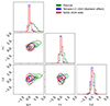 |
Fig. A.1. Comparison between the SDSS quasar g − r, r − i and i − z colours (red contours), the PROSPECTOR-β colours with the Nenkova et al. 2008a,b templates (green contours), and the PROSPECTOR-β colours with the Temple et al. (2021) templates (blue contours). |
Appendix B: Photometric noise impact on SOM cell assignment algorithm
Photometric noise may impact the SOM cell assignment as shown in McCullough et al. (2024). To test how much our conclusions on the fraction of cell change are impacted by photometric noise, we introduced COSMOS2020-like photometric errors in the cell assignment algorithm. We find that adding the median COSMOS2020 photometric errors change the fractions of galaxies each component moves to a different cell by at most 1 − 2%. This implies that the variation in the SOM cell assignment we see is completely driven by the galaxy population colour variation and that a survey with COSMOS-like photometric precision, for instance Rubin-LSST (see Appendix C), is introducing a noise in the assignment algorithm that is not impacting the conclusions we see in this work.
Appendix C: COSMOS2020 and Rubin-LSST simulated photometric depths
The COSMOS2020 (Weaver et al. 2022) reference photometric redshift catalogue contains homogeneous and robust multi-wavelength photometry for a sample of 1.7 million sources. In our work, we used the photometric errors of the COSMOS2020 catalogue as representatives of the ones expected for Rubin-LSST data. In order to support this claim, we compared the depths at 3σ measured in a 3″ diameter aperture shown in Fig. 3 of Weaver et al. (2022) with those generated using the LSST Error model described in Appendix B of Crenshaw et al. (2024). The latter depths refer to coadded images for stationary sources after 10 years. The Rubin-LSST g, r, i, z, y bands depths are similar to the ones in Fig. 3 of Weaver et al. (2022), while the Rubin-LSST u-band depth is roughly one magnitude shallower than the COSMOS2020 one.
All Tables
Fraction of galaxies changing SOM cell assignment as function of the SED component.
All Figures
|
Fig. 1. Distribution of physical properties of galaxies drawn from the PROSPECTOR-β model. The redshifts and stellar masses are jointly drawn from the sum of two Schechter functions (Leja et al. 2020), the star formation rates (averaged over the last 100 Myr) are computed from the non-parametric star formation histories, while the stellar metallicities are drawn from a clipped Gaussian approximating the stellar mass-stellar metallicity relationship of Gallazzi et al. (2005). |
| In the text | |
|
Fig. 2. Distribution of model colours obtained from the sample of 106 galaxies drawn from the PROSPECTOR-β model. The colours are obtained using mock apparent magnitudes in the KiDS-VIKING ugriZYJHKs bands. We display the 16th, 50th, and 84th quantile values for each colour at the top of the corresponding 1D histogram. The dotted lines in each 1D histogram are the 16th and 84th quantile values. The 2D contours enclose the 68%, 95%, and 99% of the values. |
| In the text | |
|
Fig. 3. Exemplary illustration of the directions in which a galaxy can move in colour-magnitude space when we vary a single stellar population component at a time with respect to the fiducial case (black point). We only show some of the variants that induce the most significant changes in the g − r vs. r colour-magnitude plane. |
| In the text | |
|
Fig. 4. Five different modelled observed-frame galaxy spectra belonging to intrinsically the same galaxy at z = 0.04. The black line refers to the spectrum generated with the fiducial PROSPECTOR-β model parameters, while the red, green, magenta and blue curves show the spectra generated varying the IMF (‘Salpeter IMF’), the attenuation law (‘Calzetti k(λ)’), the AGN prescription (‘Temple+21 QSO’) and removing the gas component (‘No gas emission’), keeping the other model parameters fixed. The vertical bands mark the regions where some of the most prominent emission lines appear. The emission line names are reported in black. The spectra units are not arbitrarily rescaled to highlight the effect of varying the stellar population components at fixed physical properties of galaxies on the continuum flux. |
| In the text | |
|
Fig. 5. Rest-frame colour differences between the fiducial galaxy sample (PROSPECTOR-β) and those obtained modifying one stellar population component at the time (y-axis labels). The coloured widths are the sum in quadrature of COSMOS median photometric errors in the two respective bands to indicate distinguishability on a single galaxy basis. The vertical black bars and the white dots on top of them represent the median values of each rest-frame colour difference. The light red boxes show the interquartile range (75th–25th percentile), while the whiskers represent the 84th–16th percentile ranges. |
| In the text | |
|
Fig. 6. Observed-frame colour differences between the fiducial galaxy sample (PROSPECTOR-β) and the ones obtained by modifying one stellar population component at a time. The coloured widths are the sum in quadrature of COSMOS median photometric errors in the two respective bands to indicate distinguishability on a single galaxy basis. The vertical black bars and white dots on top of them represent the median values of each observed-frame colour difference. The light red boxes show the interquartile ranges (75th–25th percentiles), while the whiskers represent the 84th–16th percentile ranges. |
| In the text | |
|
Fig. 7. Distributions of the relative difference in the cell occupation number (left panel) and in the cell mean redshift (right panel) with respect to the fiducial case. For each pair of fiducial and variable component model, we consider only the cells that are populated by both galaxy samples. The relative differences in the cell occupation number are shown as (Nj, comp − Nj, fiducial)/Nj, fiducial for clarity. The black vertical bars and the white dots on top of them represent the median value of (Nj, comp − Nj, fiducial)/Nj, fiducial, the boxes represent the 75th–25th percentile ranges and the whiskers represent the 84th–16th percentile ranges. The light green and light blue areas show the regions where the relative difference is within −0.1 ≤ (Nj, comp − Nj, fiducial)/Nj, fiducial ≤ 0.1 and −0.01 ≤ (Nj, comp − Nj, fiducial)/Nj, fiducial ≤ 0.01, respectively. The right panel shows the distributions of the differences in the mean redshift per cell between the fiducial case and the SED components variation cases normalised by 1 + z. The elements on the plot have the same meaning, but the light green and light blue areas show instead the regions where the relative difference of cell mean redshift is within |
| In the text | |
|
Fig. 8. Differences |
| In the text | |
|
Fig. 9. Redshift distribution N(z) of two sets of five tomographic bins built with the prescription highlighted in Sect. 6. The filled histograms refer to the N(z)s built with the fiducial sample, while the histograms with the dashed outlines represent the N(z)s built using the ‘Calzetti k(λ)’ component. The solid and dashed vertical lines represent the mean of the tomographic bins for the fiducial and the ‘Calzetti k(λ)’ components, respectively. The legend shows the tomographic bin means and 1σ errors on the means. We use the ‘Calzetti k(λ)’ component to demonstrate our analysis methodology as it induces the largest shift in the N(z). The shift is caused by the brighter rest-frame UV emission that the ‘Calzetti k(λ)’ component induces (see Fig. 4). This leaves the low-redshift galaxy observables unaffected, while it brightens high-redshift galaxies in the observed optical bands, hence making them more numerous in a magnitude-limited sample. |
| In the text | |
|
Fig. 10. Impact of varying the choices of the SED modelling component on the mean of the tomographic redshift distribution bins. Each panel shows a different tomographic bin, from the lowest (left-most) to the highest (right-most) redshift one. Each row represents a different SED modelling component we vary. The scatter points represent the difference between the mean redshift per bin obtained with the fiducial PROSPECTOR-β model and that obtained by varying one SED modelling component at the time. Orange scatter points are obtained by weighting the P(z|ci) for the number of simulated galaxies per SOM cell, while light blue points are obtained by weighting the P(z|ci) for the observed abundances in the Masters et al. (2015), McCullough et al. (2024) SOM cells. Circle-shaped, star-shaped and diamond-shaped scatter points refer to the cases where we perform an i-band magnitude-selection of the sample of galaxies that is different for each component, matched for the total number of galaxies and based on the fiducial i-band distribution, respectively. We report the mean errors on the difference of the tomographic bin means estimated via bootstrap resampling in the black boxes in the bottom right-hand corner of each subplot. The blue and red coloured bands refer to the Rubin-LSST Y10 galaxy clustering and weak lensing requirements, respectively. |
| In the text | |
|
Fig. 11. Impact of varying the choices of the SED modelling component on the scatter of the tomographic redshift distribution bins. Each panel shows a different tomographic bin, from the lowest (left-most) to the highest (right-most) redshift one. Each row represents a different SED modelling component we vary. The scatter points represent the difference between the redshift scatter per bin obtained with the fiducial PROSPECTOR-β model and that obtained by varying one SED modelling component at the time. The orange scatter points are obtained by weighting the P(z|ci) for the number of simulated galaxies per SOM cell, while the light blue points are obtained by weighting the P(z|ci) for the observed abundances in the Masters et al. (2015), McCullough et al. (2024) SOM cells. Circle-shaped, star-shaped and diamond-shaped scatter points refer to the cases where we perform an i-band magnitude-selection of the sample of galaxies that is different for each component, matched for the total number of galaxies and based on the fiducial i-band distribution, respectively. We report the mean errors on the difference of the tomographic bin scatters estimated via bootstrap resampling in the black boxes in the bottom right-hand corner of each subplot. The blue and red coloured bands refer to the Rubin-LSST Y10 galaxy clustering and weak lensing requirements, respectively. |
| In the text | |
|
Fig. A.1. Comparison between the SDSS quasar g − r, r − i and i − z colours (red contours), the PROSPECTOR-β colours with the Nenkova et al. 2008a,b templates (green contours), and the PROSPECTOR-β colours with the Temple et al. (2021) templates (blue contours). |
| In the text | |
Current usage metrics show cumulative count of Article Views (full-text article views including HTML views, PDF and ePub downloads, according to the available data) and Abstracts Views on Vision4Press platform.
Data correspond to usage on the plateform after 2015. The current usage metrics is available 48-96 hours after online publication and is updated daily on week days.
Initial download of the metrics may take a while.