| Issue |
A&A
Volume 692, December 2024
|
|
|---|---|---|
| Article Number | A18 | |
| Number of page(s) | 18 | |
| Section | The Sun and the Heliosphere | |
| DOI | https://doi.org/10.1051/0004-6361/202450680 | |
| Published online | 29 November 2024 | |
Exploring the time variability of the solar wind using LOFAR pulsar data
1
Physics, School of Natural Sciences, Ollscoil na Gaillimhe – University of Galway, University Road, Galway H91 TK33, Ireland
2
Dipartimento di Fisica “G. Occhialini”, Universitá degli Studi di Milano-Bicocca, Piazza della Scienza 3, 20126 Milano, Italy
3
INFN, Sezione di Milano-Bicocca, Piazza della Scienza 3, 20126 Milano, Italy
4
INAF – Osservatorio Astronomico di Cagliari, via della Scienza 5, 09047 Selargius, (CA), Italy
5
School of Physics, Trinity College Dublin, College Green, Dublin 2 D02 PN40, Ireland
6
Florida Space Institute, University of Central Florida, 12354 Research Parkway, Partnership 1 Building, Suite 214, Orlando, 32826-0650 FL, USA
7
Oregon State University, 1500 SW Jefferson Ave, Corvallis, OR 97331, USA
8
Max-Planck-Institut für Radioastronomie, Auf dem Hügel 69, 53121 Bonn, Germany
9
Fakultät für Physik, Universität Bielefeld, Postfach 100131, 33501 Bielefeld, Germany
10
National Centre for Radio Astrophysics, Pune University Campus Pune 411007, India
11
Dipartimento di Fisica, Università di Cagliari, Cittadella Universitaria, I-09042 Monserrato, (CA), Italy
12
LPC2E – Université d’Orléans/CNRS, 45071 Orléans Cedex 2, France
13
Observatoire Radioastronomique de Nançay (ORN), Observatoire de Paris, Université PSL, Univ Orléans, CNRS, 18330 Nançay, France
14
Jodrell Bank Centre for Astrophysics, Department of Physics and Astronomy, University of Manchester, Manchester M13 9PL, UK
15
Australia Telescope National Facility, CSIRO, Space and Astronomy, PO Box 76 Epping, NSW 1710, Australia
16
SKA Observatory, Jodrell Bank, Lower Withington, Macclesfield SK11 9FT, United Kingdom
17
Department of Physics and Astronomy, University of the Western Cape, Bellville, Cape Town 7535, South Africa
18
Leibniz Institute for Agricultural Engineering and Bioeconomy (ATB), Max-Eyth-Allee 100, 14469 Potsdam, Germany
19
University of Hamburg, Gojenbergsweg 112, 21029 Hamburg, Germany
20
Max Planck Institute for Astrophysics, Karl-Schwarzschild-Str. 1, 85741 Garching, Germany
21
Ruhr University Bochum, Faculty of Physics and Astronomy, Astronomical Institute (AIRUB), 44780 Bochum, Germany
22
Thüringer Landessternwarte Tautenburg, Sternwarte, 507778 Tautenburg, Germany
23
Leibniz Institute of Astrophysics, An d. Sternwarte 16, 14482 Potsdam, Germany
⋆ Corresponding author; This email address is being protected from spambots. You need JavaScript enabled to view it.
Received:
10
May
2024
Accepted:
14
September
2024
Abstract
Context. High-precision pulsar timing is highly dependent on the precise and accurate modelling of any effects that can potentially impact the data. In particular, effects that contain stochastic elements contribute to some level of corruption and complexity in the analysis of pulsar-timing data. It has been shown that commonly used solar wind models do not accurately account for variability in the amplitude of the solar wind on both short and long timescales.
Aims. In this study, we test and validate a new, cutting-edge solar wind modelling method included in the enterprise software suite (widely used for pulsar noise analysis) through extended simulations. We use it to investigate temporal variability in LOFAR data. Our model testing scheme in itself provides an invaluable asset for pulsar timing array (PTA) experiments. Since, improperly accounting for the solar wind signature in pulsar data can induce false-positive signals, it is of fundamental importance to include in any such investigations.
Methods. We employed a Bayesian approach utilising a continuously varying Gaussian process to model the solar wind. It uses a spherical approximation that modulates the electron density. This method, which we refer to as a solar wind Gaussian process (SWGP), has been integrated into existing noise analysis software, specifically enterprise. Our Validation of this model was performed through simulations. We then conduct noise analysis on eight pulsars from the LOFAR dataset, with most pulsars having a time span of ∼11 years encompassing one full solar activity cycle. Furthermore, we derived the electron densities from the dispersion measure values obtained by the SWGP model.
Results. Our analysis reveals a strong correlation between the electron density at 1 AU and the ecliptic latitude (ELAT) of the pulsar. Pulsars with |ELAT|< 3° exhibit significantly higher average electron densities. Furthermore, we observed distinct temporal patterns in the electron densities in different pulsars. In particular, pulsars within |ELAT|< 3° exhibit similar temporal variations, while the electron densities of those outside this range correlate with the solar activity cycle. Notably, some pulsars exhibit sensitivity to the solar wind up to 45° away from the Sun in LOFAR data.
Conclusions. The continuous variability in electron density offered in this model represents a substantial improvement over previous models, that assume a single value for piece-wise bins of time. This advancement holds promise for solar wind modelling in future International Pulsar Timing Array (IPTA) data combinations.
Key words: gravitational waves / methods: data analysis / solar wind / pulsars: general
© The Authors 2024
 Open Access article, published by EDP Sciences, under the terms of the Creative Commons Attribution License (https://creativecommons.org/licenses/by/4.0), which permits unrestricted use, distribution, and reproduction in any medium, provided the original work is properly cited.
This article is published in open access under the Subscribe to Open model. This email address is being protected from spambots. You need JavaScript enabled to view it. to support open access publication.
1. Introduction
The solar wind (SW) is a highly magnetised stream of plasma propagating in interplanetary space from the hot solar corona, first mentioned in Biermann (1951). The composition of the SW is a mixture of materials found in the solar plasma, composed of ionised hydrogen (electrons and protons) with an 8% component of ionised helium (also called α particles) and trace amounts of heavy ions and atomic nuclei (e.g. Feldman et al. 1998). The Ulysses spacecraft (Marsden & Wenzel 1991), with its near-polar orbit, has revealed that the SW exists in a bimodal state: an irregular and dense slow wind with typical speeds of ∼400 km/s and a smooth fast wind with a speed of ∼750 km/s (Issautier et al. 2003). This fast wind has been shown to originate from coronal holes and the slow wind from the boundaries or interiors of streamers (see e.g. Fig. 1 in Tiburzi et al. 2019).
Pulsars are rapidly rotating neutron stars mainly visible as regularly pulsating radio sources. Their rotation is so reliable that it can be used as a highly precise clock-like signal. By studying this clock signal, via their emitted radio pulses, pulsars can be used to probe several effects, such as interstellar weather associated with the SW. This is done by measuring the electron content of the heliosphere, due to SW-induced modifications on a given pulsar’s transiting radio pulse, also known as dispersion. These modifications are quantified using a metric defined as the dispersion measure (DM), namely the integral of the column density of free electrons  along the line of sight (LoS):
 (1)
(1)
Dispersion causes a delay in the arrival of pulsar emission that depends on the frequency of the radiation and the DM parameter (measured in pc cm−3). This delay can be written as:
 (2)
(2)
where  is the dispersion constant and ν is the observing frequency (Kulkarni 2020). Equation (1) shows that the DM can vary because of changes in electron density along a given LoS. These changes can be tracked thanks to the inverse-square dependency on the observing frequency, with pulsar observations collected with low-frequency facilities being particularly sensitive to this effect. The measured DM features components related to both the SW and changes in the ionised interstellar medium (IISM), which have differing time-varying signatures that can be used to disentangle the two components.
The DM parameter can be calculated via a process called pulsar timing (e.g. Lorimer & Kramer 2004). This involves monitoring the arrival times of radio pulses from a pulsar at an observatory. These times of arrival (ToAs) are converted to solar system barycentric arrival times for analysis in an inertial reference frame. A mathematical model based on an ensemble of pulsar characteristics, also known as the timing model (TM), is then used to compare and quantify factors affecting the ToAs. This technique enables precise measurement of the pulsar parameters on which the TM is based, with accuracy increasing with longer data sets and improved ToA measurements. Different phenomena introduce noise in the timing residuals (the difference between the observed ToAs and the arrival times predicted by the TM), such as gravitational waves (GWs). Some of these noise sources can be accurately characterised by measuring the correlated signatures in the residuals in an array of pulsars. This is done by using decades of observations of several millisecond pulsars (MSPs, Backer et al. 1982) observed using different telescopes. This experimental methodology forms the basis for a pulsar timing array (PTA). Several PTA collaborations like the European Pulsar Timing Array (EPTA, Antoniadis et al. 2023b), North American Nano-hertz Observatory for Gravitational Waves (NANOGrav, Swiggum & NANOGrav Pfc 2022), Parkes Pulsar Timing Array (PPTA, Zic et al. 2023) and Indian Pulsar Timing Array (InPTA, Tarafdar et al. 2022) have been combining their datasets to form a global consortium called International Pulsar Timing Array (IPTA). Their aim is to obtain a clear detection of the gravitational wave background (GWB, Hellings & Downs 1983). In 2023, PTAs such as the EPTA+InPTA, NANOGrav and the PPTA collaborations (see e.g. Antoniadis et al. 2023a; Agazie et al. 2023; Reardon et al. 2023) identified a correlated signature consistent with a GWB at a confidence level of at least 3σ. A variety of noise sources can induce a false detection of the GWB. One such noise source in PTAs is the SW as described by Tiburzi et al. (2015). Hence, it is essential to fully understand its contribution to the TM solutions to optimise the recovery of any underlying GWB signals.
Several studies have been carried out to observe the SW using pulsars (e.g. Counselman & Rankin 1972; Madison et al. 2019; Tokumaru et al. 2020; Tiburzi et al. 2021; Kumar et al. 2022). It is worth noting that SW can change the DM by a measure of approximately 0.01 pc cm−3 for the MSPs whose LoS gets close to the Sun. In reality, for most pulsars it is one order of magnitude smaller and these contributions become important as they are time variable and the current precision of the DMs achieved in the low-frequency observation is much smaller than the DM contribution by SW (see for e.g. Donner et al. 2020). The standard approach in pulsar timing is to model the SW as a time-independent spherical distribution of free electrons, where the DM varies according to the following equation:
![Mathematical equation: $$ \begin{aligned} \mathrm{DM}_{\rm {SW}} = n_{\rm e}\frac{\rho }{r_{\rm e} \sin \rho }[1\,\mathrm{AU} ]^2, \end{aligned} $$](/articles/aa/full_html/2024/12/aa50680-24/aa50680-24-eq5.gif) (3)
(3)
Here, ρ is the pulsar-Sun-observer angle, ne is the electron density at 1 AU and re is the distance between the observatory and the Sun (Tiburzi et al. 2019). You et al. (2007b) proposed an alternative model that took into account the bimodal nature of the SW. They used distinct radial distributions of free electrons for each of the two streams within the SW, fast and slow, and utilised solar magnetograms obtained from the Wilcox observatory1 to differentiate the LoS components that had been influenced by one stream or the other. The total contribution of the SW was obtained by adding these individual contributions.
Both of these models have shortcomings, as demonstrated by Tiburzi et al. (2019), who formally compared the performance of the two approaches, in addition to adding a time-variable amplitude to the spherical model, using low-frequency observations of the binary radio MSP PSR J0034−0534. This work showed that neither model provided a satisfactory description of the SW effects on the dataset, although the spherical model performed systematically better than the bimodal one, in contrast to the conclusions of You et al. (2007b). The observed inconsistency between the You et al. (2007b) and Tiburzi et al. (2019) analyses is believed to stem from either of the following: (i) the enhanced precision in DM reached thanks to the lower observing frequency in the dataset utilised by Tiburzi et al. (2019) in contrast to that employed by You et al. (2007b); or (ii) a potential difference in the effectiveness of the two-phase model concerning the heliospheric latitude of the pulsar, as both the studies examined data from different pulsars. In the same year, (Madison et al. 2019) found the optimal value of ne to be 7.9 ± 0.2 cm−3 via an analysis of the NANOGrav 11-yr dataset (Arzoumanian et al. 2018). However, it was noted that this value could be significantly improved if one used a lower observing frequency and larger temporal baseline. Tiburzi et al. (2021) subsequently showed that a time-variable SW amplitude is a better description of the SW signal in pulsar data, compared to a constant one as previously used. Working in the context of PTAs, Hazboun et al. (2022) demonstrated that by relaxing the assumption that the electron density around the Sun drops off as 1/r2, and by assuming a more general electron density decreasing as 1/rγ, improved results could be achieved. They also compared the use of a piece-wise binned time dependence for ne to a deterministic Fourier-basis model, both used in order to more easily model the time dependence across multiple pulsars. A recent study by Nitu et al. (2024) has examined the effectiveness of Gaussian processes on estimating the effect the SW has on pulsar pulse dispersion. The authors showed that fitting for a piece-wise function for each solar conjunction using Gaussian Processes effectively encapsulates the variability associated with the SW. Whilst these authors presented an annual single value fit for the ne, we note that this does not take into account the continuous variability of SW electron densities which has been observed by numerous ‘in situ’ spacecraft operating in the inner solar system.
Ongoing efforts to incorporate low-frequency radio data from the LOw-Frequency ARray (LOFAR, van Haarlem et al. 2013) telescopes into the upcoming IPTA data release are underway. Therefore, modelling the impact of the SW-associated dispersion on TMs is of key significance as their effect is strongly pronounced in this data set, making it imperative to model this noise source accurately and formally integrating a functioning SW noise model into the existing noise analysis packages, for instance, enterprise (Taylor et al. 2021).
In this study, we present the solar wind Gaussian process (SWGP), a method developed and tested by the authors, and integrated into enterprise_extensions (Taylor et al. 2021) to account for the time-variability of the dispersion associated with the SW. SWGP uses Bayesian analysis techniques to examine the SW structure within the context of pulsar timing. First, we describe how simulations are used to assess the performance of the model. After this tuning phase, we then apply the model to pulsar data obtained with LOFAR. A total of eight pulsars are considered in our investigation, numerically increasing the sample used in Nitu et al. (2024), in which only three pulsars were considered. We demonstrate the improvement of this approach over previous methods, such as that employed by Tiburzi et al. (2021). Furthermore, we explore evidence for SW-associated variability with changing ecliptic latitudes and we also compare the derived ne values obtained from the pulsars with ‘in situ’ measurements from spacecraft. We confirm that the study of the heliospheric SW using radio pulsars is capable of resolving the two-phase structure of SW, confirmed by data obtained from the Ulysses mission. We also discuss the viability of considering the SW contribution as a common noise source when performing the TM analyses as part of the formal IPTA analysis workflow to detect GWB signatures.
This paper is divided into the following sections. In Sect. 2, we describe the model and provide its theoretical background and context. In Sect. 3, we show the performance of the described model on simulations. We describe the pulsar timing dataset, and how it was obtained, in Sect. 4. Our modelling methods are applied to these data in Sect. 5, along with our results. In Sect. 6 we test the viability of using SW as a common noise, before presenting our conclusions in Sect. 7.
2. Methodology and tools
In this section, we briefly describe the models we used for each noise process. All the models described in this section have been incorporated in the enterprise software suite (Ellis et al. 2019). We explain the Bayesian framework that is used in this paper and the definitions of Gaussian likelihood, along with a descriptions of the theoretical basis for each of the models used as part of the data analysis in this study.
2.1. Bayesian framework and likelihood
The methodology of this paper is primarily based on the Bayesian approach to parameter inference. The physical imprints that are embedded in the timing residuals can be characterised by several parameters. All these parameters are considered as random variables, and their associated probability distribution functions are calculated according to the Bayes theorem for each of those parameters. In our case, we assume that the noise in the timing residuals are characterised by various parameters that are listed in Table 1. The priors of each of the parameters are sampled according to Gaussian Processes (GP). GPs are used to model stochastic variations such that every finite collection of the random variables follow a multivariate normal distribution (Rasmussen & Williams 2006).
Parameter list with the corresponding priors.
The timing residuals (δt) contain two kinds of components namely, stochastic and deterministic. The Gaussian likelihood for the timing residuals can be defined in the time domain as:
![Mathematical equation: $$ \begin{aligned} \begin{aligned} L&(\delta t|\theta _d,\theta _s) =\\&\frac{\mathrm{exp}\left[-\frac{1}{2}\sum _{ij}\bigg (\delta t_i - \mathcal{D} (t_i;\theta _d)\bigg )^{T} \boldsymbol{C}_{ij}^{-1}(\theta _s)\bigg (\delta t_j - \mathcal{D} (t_j;\theta _d)\bigg )\right]}{\sqrt{(2\pi )^n|\boldsymbol{C}|}} , \end{aligned} \end{aligned} $$](/articles/aa/full_html/2024/12/aa50680-24/aa50680-24-eq8.gif) (4)
(4)
where i, j ∈ {1, 2, …, n}, n being the number of ToAs. 𝒟 is the time domain function representing any deterministic signal, C is the time domain covariance matrix, where the stochastic signals are included. They are parameterised by θd and θs respectively (van Haasteren et al. 2009). In this work, 𝒟 corresponds to the deterministic parameter, namely the electron density at 1 AU from the SW which is represented by  . More details on the deterministic component are presented in Sect. 2.6.
The general covariance matrix is decomposed into the following stochastic components:
 (5)
(5)
where each term represents the covariance matrix corresponding to timing model errors, white noise, DM noise, red noise and time variable SW respectively. All of these noise components are described in the following subsections.
2.2. Timing model marginalisation
In conventional practice, the assumption of the best-fit timing solution only comprising radiometer noise tends to over-fit the overall solution which can introduce bias towards other unmodelled sources. To address this, fitting all parameters in the timing model as Bayesian hyperparameters within the enterprise package has been considered. However, this method is inefficient as it can be computationally expensive. An alternative approach involves analytically marginalising the likelihood over the errors associated with timing model parameters (Chalumeau et al. 2021). It has been demonstrated by Van Haasteren & Vallisneri (2014) that this process is equivalent to the marginalisation of a corresponding Gaussian process with an improper prior. The covariance matrix for timing model errors can be defined as follows:
 (6)
(6)
where M is the design matrix, which contains the partial derivatives of the timing residuals with respect to the timing model parameters, and Σ = λI where I is the identity matrix and λ is a large numerical constant. We note that the covariance matrix, CTMe, does not contain any parameter to fit for. It is a way to marginalise over the TM errors, which inherently assumes a linear model of all the parameters in the TM.
2.3. White noise
A predominant element observed in pulsar timing data is white noise (WN), distinguished by its stochastic fluctuations and the absence of obvious periodic patterns. This is generally caused by the radiometer noise from the instruments and from pulse jitter noise (Liu et al. 2012; Wang 2015). The ToAs are calculated using cross-correlation between the template profile and the integrated pulse profile at distinct epochs. Due to the presence of WN, we can redefine the uncertainties in the ToAs that are quantified by their ToA errors (σToA), which can be adjusted as follows:
 (7)
(7)
Here, σ represents the new uncertainty after accounting for WN, Ef (or EFAC) is the multiplicative factor that is attributed to the uncertainty related to radiometer noise, while Eq or EQUAD accounts for various stochastic noises such as profile variations by adding in quadrature. As a result, the WN covariance matrix, (CWN) is given by:
 (8)
(8)
where i and j indices denote corresponding backend’s ToAs. Then, δij representing the Kronecker delta function; EFAC and EQUAD serve as empirical parameters characterising white noise for each system (Chalumeau et al. 2021).
2.4. Red signals
Red signals are noise processes with an associated ‘red’ power spectrum, that is, dominated by low frequencies. It is essential to model such red noise signals, as they can have similar signature as that of nano-hertz gravitational waves within PTA timing solution data. A study by Hazboun et al. (2020) clearly demonstrated the need to model these signals accurately to ensure recovery of valid GWB detection. Similar to Chalumeau et al. (2021), we adopt a function-space view of the Gaussian process. The timing residuals due to the red signals at each epoch, ti, are modelled as
 (9)
(9)
where Xl and Yl play the role of weights and the Fourier basis functions are:
 (10)
(10)
where l = 1, 2, …, N. Here, N represents the number of Fourier components. This representation aligns with the conventional Fourier transform under the condition that f = l/T (where T denotes the total time span) in the scenario of evenly spaced observing epochs, ti. However, in our dataset, observations tend to be irregular with an uneven cadence, leading to the non-orthogonality of the Fourier bases. Nonetheless, for this study, we adopt a set of evenly spaced frequencies Δf = 1/T, commencing at f = 1/T and terminating at N/T.
The covariance matrix Σ governing the Fourier coefficients is determined by the power spectral density (PSD) S(f), with the simplest model being a power law:
 (11)
(11)
described with parameters θs = (A, γ), where the amplitude A is the normalised value at the frequency of  , and γ is the spectral index. The covariance matrix in the frequency domain is thus given by
 (12)
(12)
where k, l = 1, 2, ....,N. For our purposes, we consider only spatially uncorrelated red signals.
2.4.1. Achromatic red noise
Achromatic red noise (RN) is widely used in single-pulsar noise models to depict the long-term variation of the pulsar spin. Also known as ‘timing noise’ or ‘spin noise’, RN significantly affects ToAs in younger pulsars, and various physical mechanisms have been proposed to explain it, including magnetospheric variability and interactions between the superfluid core of the pulsar and the solid crust (Alpar et al. 1986; Hobbs et al. 2006b). The origins of RN in MSPs may differ from those in young pulsars due to their substantially weaker magnetic fields; superfluid turbulence in the stellar interior has been suggested as a potential contributor to RN in MSPs (Melatos & Link 2013). We modelled the RN according to the description given above. This noise component is unique for each pulsar. Furthermore, it is not radio-frequency dependent, and is spatially uncorrelated among different pulsars. The RN covariance matrix is
 (13)
(13)
where FRN is the Fourier basis functions as they are detailed in Eq. (10) and ΣRN is the covariance matrix in the frequency domain.
2.4.2. Chromatic red noise
Chromatic red noise or DM noise is caused by the plasma along the pulsar’s LoS, including contributions from the interstellar medium (ISM), the solar system interplanetary medium, and the terrestrial ionosphere. As the pulsar signal travels to the observatory, it gets dispersed by all the plasma along the LoS, which causes a time delay scaling as Δt ∝ ν−2. The most prominent contribution to this dispersive delay typically comes from the ISM. As mentioned, this time delay is quantified by the DM parameter, that can vary because of variations in the LoS, causing time-correlated noise in the timing residuals, such variability needs to be quantified so as not to obscure GWB detection (Keith et al. 2013; You et al. 2007a). We used a similar model to describe the DM variations (henceforth known as DMv) as for the achromatic red noise.
We model DM noise as a power law with parameters ADM and γDM, with Fourier basis components, FDM ∝ κj, where κj = K2νj−2 is introduced to model the dependence of DM noise amplitude on the radio frequency νj of ToA j (Van Haasteren & Vallisneri 2014). We choose K = 1400 MHz to be the reference frequency in our case. The covariance matrix for DM noise can be expressed as:
 (14)
(14)
where the FDM values represent the Fourier basis functions of the DM noise and ΣDM, ISM is the covariance matrix in the frequency domain for DM noise, detailed in Eq. (12). We note that the presence of other chromatic effects such as frequency-dependent dispersion is negligible (as stated in Donner et al. 2020). Furthermore, the effects of ionosphere are extremely tiny when compared with the effects of IISM. So, the modelling of chromatic red noise inherently covers the modelling of ionosphere. For context, the DM contribution due to ionosphere is generally of the order of 1e−5 pc cm−3 (see Eq. (22) in Bray et al. 2015), which is much smaller than both the SW and IISM effects. Thus, in this study, we neglected ionosphere effects substantial enough to require a separate modelling.
2.5. solar wind Gaussian process
The solar wind Gaussian process (SWGP) is a noise model included in the enterprise_extensions2 chromatic noise analysis module that we test here for the first time. It adopts a power spectral density achieved through a power-law formulation, similarly to Eq. (11):
 (15)
(15)
where SPSW is power-law spectral density for SWGP, ASW is the amplitude of the solar wind at 1/1 yr frequency, f the spectral frequency and γSW is the spectral index of secular SW variations.
The Fourier basis components for SWGP are modulated by the spherical model to account for secular SW variations. Thus, the Fourier components can be expressed as
 (16)
(16)
where l = 1, 2, …, N. Here, N represents the number of Fourier components considered, FRN represents the Fourier components for Red Noise which are formulated according to Eq. (10), ν is the observing frequency, and DMSW, ne = 1 is the DM due to SW (see Eq. (3)) when calculated with ne = 1.0. This multiplication is needed to effect the impact of the changing LoS impact parameter throughout the year as shown in Fig. 1. Using Eqs. (15) and (16), the corresponding time-domain covariance matrix for SWGP can be written as:
 (17)
(17)
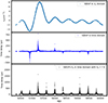 |
Fig. 1. Sample results from one SWGP realisation. In a hypothetical scenario, considering the long time span of one of the pulsars in our dataset PSR J1022+1001. The top panel shows the variations in ne that can be modelled using SWGP perturbed from the mean value. The middle panel shows the corresponding time delays due to SWGP. The bottom panel shows the time delay when the deterministic signal with an |

Here, FSW represents the Fourier basis functions as detailed in Eq. (16), θs = (ASW, γSW) and  is the covariance matrix in frequency domain (which is expressed as in Eq. (12)). The Fourier components are equally spaced within the frequency range from 1/T to N/T, with frequency bins truncated at
  . This truncation implies that the SWGP primarily accounts for the lower frequency bins up to the truncation limit, focusing on modelling long-term variations in the solar wind while ignoring shorter timescale variations. This was implemented into the model due to various reasons. Firstly, the long-term variations in the SW primarily show a cycle of 11 years and at higher frequencies degrade into a red-noise turbulence spectrum. Due to the Gaussian measurement noise present in our data, we generally do not have any sensitivity to SW variations at higher frequencies, where they have power below our noise floor. Secondly, since our data are effectively only sensitive to the SW during a solar conjunction (and few weeks before and after), variations occuring on timescales faster than
  cannot generally be reliably measured. Finally, one important heliospheric component that could be significantly measured in our data at shorter timescales, are coronal mass ejections (CMEs). In practice, observations affected by CMEs are treated as outliers in long-term pulsar timing studies and are thus excluded from the analysis. Consequently, the effect of shorter timescale variations on the timing residuals is minimal and does not significantly impact the results.
2.6. Deterministic signal
While previous subsections addressed stochastic noise processes, here we focus on the deterministic noise component of our model. In addition to the secular variations in the solar wind density modelled in Sect. 2.5, our model includes a time-constant, average solar-wind signature quantified by the parameter  , sampled according to the spherical model described by Eq. (3). When combined with the variations quantified by the SWGP term, this fully describes the impact of the solar wind on the pulsar timing observations. Figure 1 demonstrates how this average term and the variable SWGP terms compare, based on the example of PSR J1022+1001: the top panel shows the time-varying electron density Δne modelled by the SWGP. Since the impact of this parameter on the timing depends on the solar angle (see Eq. (3)), the variations in the top panel result in timing delays shown in the middle panel of Fig. 1. Since SWGP only models the time-variable component of the solar wind, it can go both positive and negative. However, in combination with a constant,
  of 7.9 cm−3, the corresponding time delays are depicted in the bottom panel. The equation for the deterministic component of the signal is as follows:
![Mathematical equation: $$ \begin{aligned} \mathcal{D} (t_i,\nu _i;\bar{n}_{\rm e}) = \bar{n}_{\rm e}\frac{\rho (t_i)\ [\mathrm 1\,AU ]^2}{r_{\rm e}(t_i) \sin [\rho (t_i)]} \frac{1}{ K_D \nu _i^2}, \end{aligned} $$](/articles/aa/full_html/2024/12/aa50680-24/aa50680-24-eq30.gif) (18)
(18)
where ti is the observing epoch, ρ(ti), re(ti) and νi represent the pulsar-Sun-observer angle, the distance between the observatory and Sun and observing frequency at ti respectively. KD is the dispersion constant (see Eq. (2)). Henceforth, we note that ne refers to the varying electron density at 1 AU whereas,  refers to the average electron density at 1 AU.
2.7. Software
In this subsection, we describe the tools that are used in this study.
TEMPO2 and libstempo. TEMPO2 (Hobbs et al. 2006a; Edwards et al. 2006) is a software package utilised for the analysis of pulsar ToAs. TEMPO2 accounts for various effects using different parameters. It facilitates fitting for different parameters using the timing model. libstempo3 is a Python wrapper of TEMPO2. This package provides the same functionalities as TEMPO2, with the added advantage of seamless integration with other Python-based software. In this work, libstempo has been employed to simulate residuals to evaluate the SW model detailed in Sect. 3.
enterprise & enterprise_extensions. This package has been developed to model the noise processes in the timing residuals based in python. All the noise models that are used in this study are embedded into this software. We use a PTMCMCsampler4 to conduct the Markov chain Monte Carlo sampling.
laforge. laforge5 (Hazboun 2020) is used to create time-domain realisations from the models defined in enterprise that are parameterised in the frequency domain. In this study, we applied this method to various noise models such as achromatic red noise, DM noise and SWGP. A detailed description of this package is in Iraci et al. (in prep.).
3. Simulations
We tested the SWGP implementation described in Sect. 2.5 on simulated ToA datasets using libstempo. In particular, we generated noise-free ToAs with SW signal. To introduce statistical errors, we injected reasonable amount of white noise into the simulations which is detailed in each scenario for simulations. Furthermore, to make the simulations more realistic, we injected RN and DM noise with probability distribution that is a power-law in form. The corresponding amplitudes and slopes for RN and DM noise were drawn from probability distributions well established literature (see e.g. Goncharov et al. 2020).
The observational characteristics of these simulations were specifically tailored to those of the LOFAR telescope. This means an acquisition cadence spanning approximately 3 to 5 days, and a radio-frequency coverage from 110 to 190 MHz with 10 sub-bands. The total temporal baseline of the simulations spans four years. The pulsar on which we based the simulations was PSR J1022+1001; this pulsar has been monitored by all PTA experiments for several decades. Its ecliptic latitude is −0.06° making it an ideal source for investigating the SW. We note that we do not consider CMEs in the simulations and other shorter term variations as they are considered as outliers in the PTA datasets as explained in Sect. 2.5. Our simulations cover four different test cases, which are detailed in the following subsections.
3.1. Simulations with yearly varying ne
In this subsection, we describe two different scenarios, with varying degrees of complexity. In scenario 1, we have a SW signal without any additional noise. In scenario 2, we attempt to include other kinds of noise such as WN, RN and DM noise.
3.1.1. Scenario 1
In the first scenario, we simulate the SW amplitude (ne) with a constant value per year, with a yearly step function centred on the solar conjunction with the pulsar; namely, four different values as shown in Fig. 2. In reality the value of ne fluctuates much more rapidly than this but for our first scenario we used this very simple description. We then used Eq. (3) to create a DM time series, subsequently, the corresponding timing residuals using Eq. (2). These steps are summarised in Fig. 2. Following a fit for a single constant value of  using TEMPO2, we can see that the post-fit residuals (Fig. 2, bottom panel) clearly demonstrate the necessity of modelling for the variability of the SW.
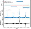 |
Fig. 2. Simulation scenario 1, only SW. Top: ne variations simulated (blue) are shown as well as the mean value (red) and the ne retrieved (green) when fit for a single value with TEMPO2. Middle: Blue points represent the residuals corresponding to the injected values of ne. Bottom: Green points represent the residuals after a constant |

3.1.2. Scenario 2
Next, to improve the noise-free scenario and make the yearly scenario more realistic, we also included three sources of noise. Those parameters are reported in Table 2.
Parameters of the noise components injected in scenario 2 of the first test case.
We then re-performed a single pulsar noise analysis using the formulation detailed in Sect. 2. We recover the noise parameters and, by using the SWGP approach, we additionally recovered the  value. The resulting posterior plot (Fig. 3) visually illustrates the fidelity of the parameter recovery, with the black lines within the posterior plot representing the noise values originally injected. With respect to the
  parameter, the black line signifies the average of all injected values of ne, as shown in Fig. 3. This indicates that the SWGP parameters effectively account for an annually-varying ne, making the recovered value of
  in the posterior chain an average of injected values.
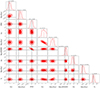 |
Fig. 3. Simulation scenario 2, with noise. Posterior chain plot for yearly varying ne scenario. The black lines represent the truth values injected into the simulations. The black line in |


To check the accuracy of this posterior parameters, we employed the laforge software package which reconstructs the Gaussian process parameters to a time-domain signal shown in Fig. 4. We note that the degree of success in recovering the DM noise varies with the amplitude of the RN process (Iraci et al., in prep.).
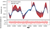 |
Fig. 4. Time domain reconstruction of the inserted simulations with various noise parameters embedded into it. It presents the specified noise parameters as in Table 2 along with the SW signal. The blue points are the simulated residuals and the orange lines are the recovery after the noise analysis. |
3.2. Simulations with continuously varying ne
In this case, the ne that we injected in the simulations was modulated on a daily basis for a period of four years, following a sine wave pattern with an 11-year periodicity to broadly mimic the solar activity cycle. Subsequently, these ne values were used to construct a DM time series, characterised by Eq. (3). Fig. 5 shows the values of ne as a function of MJD. The parameters of the other noise processes that we injected in the simulated ToAs are shown in Table 3 below.
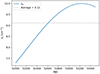 |
Fig. 5. ne plotted as a function of MJD for continuously varying SW scenario. |
Parameters of the noise components injected in the simulations that assume a continuously varying ne value.
Fig. 6 shows the time-domain reconstructed signal from the posterior chain that was obtained with a reduced χred2 of 1.46.
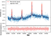 |
Fig. 6. Time domain reconstruction from the continuously varying SW scenario. |
The foregoing analyses establish the efficacy of employing SWGP for modelling varying ne value across the entire time span. The fit with TEMPO2 becomes dependent upon the number of epochs within a given solar conjunction which inherently biases the fit towards the value associated with a greater number of epochs. In contrast, modelling the variability using SWGP effectively caters to the variability, ensuring robustness in the modelling process. In the next subsection, we demonstrate the usage of SWGP on the two-phase model.
3.2.1. Extracting the electron densities at 1 AU
The cyclic nature of the Sun’s magnetic field, which undergoes reversal approximately every 11 years, induces a correlated fluctuation in the occurrence of substantial solar eruptions, such as solar flares. These eruptions emit bursts of energy and matter into space. In this scenario, our objective is to emulate these natural variations by modulating the ne. In our setup, we replicated the 11-year sine wave but with a time span of 12 years. This deliberate choice was made to encompass an entire solar activity cycle and to meticulously evaluate the ability of our simulations to accurately recover ne.
Fig. 7 illustrates the comparison between the injected DM time series and the recovered DMs obtained from posterior chain sampling SWGP. Moreover, we inverted the Eq. (3) to reconstruct the sine curve of ne injected into the simulations as follows:
 (19)
(19)
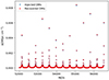 |
Fig. 7. DM time series for replicating the solar activity in ne. The blue points are injected ones, while the red points with the error bars are recovered from the noise analysis run after modelling using SWGP. |
In Fig. 8 we present the injected and recovered values of ne. The orange curve represents the injected ne curve, while the blue curve with accompanying error bars illustrates the recovered values of ne. Notably, during the solar conjunction of the pulsar, when the LoS of the pulsar is in close proximity to the Sun, the error bars diminish; this indicates an increased sensitivity to variations in the DMs induced by SW effects. Conversely, elsewhere, the error bars exhibit an oscillating pattern, with a period of 1 year, as depicted in the bottom panel of Fig. 8.
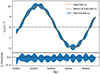 |
Fig. 8. ne recovered from the recovered DM time series in Fig. 7. The orange sine curve is the ne injected into the simulations mimicking the solar activity cycle. The black dotted line represented the average of all injected ne. |
3.3. Simulations using the two-phase model
In the third scenario, we reproduced a physical model originally presented by You et al. (2007b), which is based on the bimodal nature of the solar wind.
3.3.1. On the two phase model:
The SW can be conceptualised as comprising a quasi-static component, which exhibits a bimodal distribution and co-rotates with the Sun, and a transient component, characterised by shorter timescales ranging from hours to days. Our main focus lies on the bimodal co-rotating structure of the solar wind. This structure consists of fast and slow components, each characterised by distinct velocity and density profiles. Specifically, the density profiles are defined by the following equations:
![Mathematical equation: $$ \begin{aligned} n_{\rm e}^\mathrm{fast} =&\bigg [1.155 \times 10^{11} \bigg (\frac{R}{R_{\odot }}\bigg )^{-2} + 32.3 \times 10^{11} \bigg (\frac{R}{R_{\odot }}\bigg )^{-4.39} \nonumber \\ &+ 3254 \times 10^{11} \bigg (\frac{R}{R_{\odot }}\bigg )^{-16.25}\bigg ] m^{-3},\nonumber \end{aligned} $$](/articles/aa/full_html/2024/12/aa50680-24/aa50680-24-eq40.gif)
![Mathematical equation: $$ \begin{aligned} n_{\rm e}^\mathrm{slow} =&\bigg [2.99 \times 10^{14} \bigg (\frac{R}{R_{\odot }}\bigg )^{-16} + 1.5 \times 10^{14} \bigg (\frac{R}{R_{\odot }}\bigg )^{-6} \nonumber \\ &+ 4.1 \times 10^{11} \bigg (\bigg (\frac{R}{R_{\odot }}\bigg )^{-2} + 5.74 \bigg (\frac{R}{R_{\odot }}\bigg )^{-2.7}\bigg )\bigg ] m^{-3},\nonumber \end{aligned} $$](/articles/aa/full_html/2024/12/aa50680-24/aa50680-24-eq41.gif)
where R⊙ represents the solar radii and R is the distance from the sun expressed in solar radii (Guhathakurta & Fisher 1998; Muhleman & Anderson 1981). To compute the DM, we integrate along the LoS using Eq. (1). This model utilises Carrington rotation maps of the Sun obtained from the Wilcox solar Observatory (WSO)6 to estimate the LoS. During observation, if the LoS falls within 20° of the magnetic neutral line, it is classified as slow wind, while other regions are categorised as fast wind. Therefore, both of the phases are taken into account.
The results of these simulations have been highly useful in our understanding of the implementation of SWGP. Although acknowledging its limitations in fully capturing SW complexities (as highlighted in Tiburzi et al. 2019), it is worth noting the utility of this model in generating simulations, as it is not based on the spherical model.
3.3.2. On the implementation of simulations:
We first generated a DM time series using the bimodal structure of SW, assuming to be targeting PSR J1022+1001 for the four years of the simulation time span. Subsequently, the ToAs were derived using Eq. (2). To introduce statistical uncertainty, we injected WN into the simulations with an EFAC of 1.5 and an EQUAD of 2 × 10⁻⁶. Additionally, leveraging both the WN and SWGP components of the model, we generated a posterior chain. The exclusion of other sources of noise was deliberate, aimed at assessing the effectiveness of SWGP in modelling SW independent of a spherical model. The time domain reconstruction plot, illustrated in Fig. 9, presents our findings. Our analysis resulted in a reduced χred2 value of 2.2.
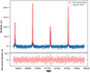 |
Fig. 9. Time domain reconstruction from the simulations when the two-phase model was used. These simulations have WN and the SW noise. |
3.4. Conclusions on simulations
The simulations demonstrate SWGP’s effectiveness. The  parameter in the posterior chain captures the constant SW signal, while SWGP parameters model the variability of the injected SW perturbed from the
  value. We apply this model to the LOFAR dataset in the following sections.
4. LOFAR dataset
The data used in this study were collected from various pulsar monitoring campaigns spanning approximately 11 years using the LOFAR core telescope (van Haarlem et al. 2013) and single station use of the German LOng Wavelength (GLOW) group7. The observing bandwidth encompasses a frequency range from 100 to 190 MHz, with a central frequency of about 150 MHz. All observations were coherently dedispersed, folded into 10-second sub-integrations and channelised in 360 frequency channels 195 kHz-wide, using the DSPSR software suite (van Straten & Bailes 2011). The integration lengths varied, ranging from 1 to 3 hours for observations conducted with the German stations (DE60X), and from 7 to 20 minutes for those conducted with the LOFAR Core telescope. In the post-processing phase, each observation was cleaned of radio-frequency interference using a modified version of the COASTGUARD software package (see Lazarus et al. 2016; Kuenkel, in prep.8) and corrected for the parallactic angle rotation and projection effects via the DREAMBEAM software package9. After this, each observation is time-averaged, and partially frequency-averaged to reach a fixed number of channels (5, 10 or 20) depending on the signal-to-noise (S/N) of the pulsar using the PSRCHIVE software suite (van Straten et al. 2011; Hotan et al. 2004).
Our analysis includes eight pulsars, that were chosen based on the following criteria:
-
Millisecond pulsar;
-
Ecliptic latitude between −15° and 15°;
-
A weekly cadence around the SW conjunction;
-
More than 4 years of observing time span;
-
Prominent SW detection in Tiburzi et al. (2021) or Donner et al. (2020).
The position of the pulsars with respect to the path of the sun for a whole year is shown in Fig. 10. For each pulsar’s observational dataset obtained from either the German stations or the LOFAR core, the ToAs were derived as follows. First, the brightest observations from a given observatory-specific dataset were time-averaged together to obtain a frequency-resolved, data-derived template of the pulse intensity as a function of the phase longitude. This was then smoothed using a wavelet-based function to obtain an essentially noise-free, frequency-resolved template using psrsmooth algorithm which is included in PSRCHIVE. A set of frequency-dependent ToAs was then obtained by cross-correlating the noiseless template with the observations themselves. In addition, a Huber-regression based routine (described in Tiburzi et al. 2019) was used to identify and reject outliers, and obtain a final series of frequency-resolved ToAs, for each observatory and for each of the selected pulsars. With these ToA series, we proceeded in applying our SWGP analysis, and we obtained the results outlined in the following section. We note that five of the eight candidates here are a subset of the study shown in Tiburzi et al. (2021). We also show the detailed properties of each pulsar in Table 4.
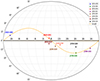 |
Fig. 10. Locations of the pulsar in reference to the Sun in equatorial coordinates. The yellow line represents the path of the Sun and the coloured dots represent the locations of each pulsar. |
Properties of each pulsar.
5. Application of SWGP to real data
Here, we describe the application of SWGP to the LOFAR dataset of Sect. 4, to account for the SW variability. For this, we need to carry out two main steps.
5.1. Optimising the components of the noise model (except for SWGP):
First, we conducted a Bayesian noise model selection on all the noise components namely the timing model parameters (also including a constant ne) using analytical marginalisation mentioned in Sect. 2.2, WN, DM noise and RN, following methods similar to those used in EPTA Collaboration (2023). We note that we considered 30 frequency bins for both RN and DM noise in the initial sampling. Initially, the parameters of the selected noise components were sampled in accordance with the methods outlined in Sect. 2. After the analysis of the resulting posterior chains, any noise process determined to be redundant (either due to its insignificance or lack of constraints) was excluded from the final noise run. Notably, it was only for PSR J1022+1001 that we discarded the RN component in the final analysis. This is because this pulsar exhibited no significant amount of RN, resulting in an unconstrained posterior. On the contrary, other pulsars have demonstrated a sensitivity to all the considered noise components. Since all the parameters for these pulsars were well constrained, we retained the choice of 30 frequency bins for RN and DM noise in the final analysis.
5.2. Optimisation of the SWGP model:
After selecting the most favoured components for the noise model, we optimised the number of frequency bins that we will use to model the SWGP spectrum in the final noise run. The default setting of the SWGP module truncates the SWGP spectrum at a frequency of 1/1.5 years (as specified in Sect. 2.5); however, for some pulsars this results in a negative output value for ne, which is non-physical. This implies that the reference cutoff frequency of 1/1.5 years is not optimal for all pulsars, hence, we optimised this by testing alternative values. We observe three pulsars for which this change is required: PSRs J0034−0534, J1400−1431 and J2256−1024. For the latter two, the optimal frequency cutoff is 1/1 year, which is motivated by the model’s preference for capturing shorter timescale variations in ne; this is possibly due to the shorter time span compared to other pulsars in our dataset. Instead, PSR J0034−0534 seems to favour the long timescale variations embedded into the first frequency bin only, 1/tspan. Further details on this pulsar are presented in Sect. 5.4. The details of the frequency bin selection is shown in Table 5.
Number of frequency bins used for each pulsar.
Once the noise analysis is completed, we used the laforge software package to isolate the SW component, namely, ASWGP, γSWGP, and  and reconstruct the corresponding DM and ne time series (the latter extracted with the method outlined in Sect. 3.2.1). These are shown, respectively, in Figs. 11 and 12.
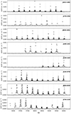 |
Fig. 11. DM time−series obtained from the changing SWGP+deterministic ne part of the posterior chain. The black points correspond to epochs with |solar_angle|< 45° from the Sun and the vertical dashed lines indicate a solar conjunction. The order of the pulsars is aligned according to their distance from the Sun in terms ecliptic latitude in ascending order. |
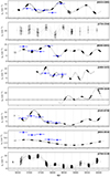 |
Fig. 12. Values of ne extracted from the DM time series shown in Fig. 11. The black points represent the epochs that have |solar_angle|< 45°. The blue points are obtained from the results presented in Tiburzi et al. (2021). The order of the pulsars is aligned according to their distance from the Sun in terms ecliptic latitude in ascending order. The long term solar cycle is evident in pulsars more than 3° away from the Sun in terms of ecliptic latitude i.e. the bottom four panels. |
5.1. Implications of SWGP for pulsar timing
In this section, we attempted to deconvolve each noise parameter which contributes to the DM parameter in the DM time series for PSR J2145−0750. In Fig. 13, the top panel consists of the DMs that are modelled using SWGP, the second panel consists of DMs due to the constant average  from the posterior and the third panel comprises of the DM time series due to the DM noise. We attempted to compare the combined DM time series from SWGP,
  and DMGP with the DM time series obtained with the Epoch-Wise10 method.
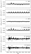 |
Fig. 13. DM time series for PSR J2145−0750 obtained with different noise elements. Top panel shows the DM reconstruction from the SWGP model. The second panel demonstrates the result from the |


This method is outlined in Tiburzi et al. (2019) and Donner et al. (2020) with the intention to obtain and study its DM time series without the need for an additional noise analysis. We note that in the DM time series shown in the fifth panel is the Epoch-Wise method after correcting for the slope in DM embedded into the timing model. The bottom panel of Fig. 13 shows the DM residuals from the Epoch-Wise method. A further demonstration of the SWGP model can be seen in Fig. 14 where we plot the DM values, using both methods, and their residuals as a function of solar angle. This highlights the SWGP model’s capability to accurately characterise the evolving effects of solar wind on pulsar timing residuals. Therefore, it appears that SWGP offers significant promise for modelling solar wind in future PTA experiments, particularly with the full integration of LOFAR and IPTA data.
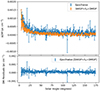 |
Fig. 14. Demonstration of SWGP model in comparison with the Epoch-wise method as a function of solar angle on PSR J2145−0750. Here, we consider the binned average over 1° of solar angle. This elucidates the working of SWGP particularly for epochs less than 30° from the Sun. |
5.2. Average electron density values
As mentioned in the previous sections, traditional pulsar timing analyses use a time-fixed spherical model to account for the SW effects with fixed values of electron density at 1 AU (4 and 9.9681 cm−3 for, respectively, tempo2 and tempo, and 7.9 cm−3 according to Madison et al. 2019). To make a comparison with this standard approach, we report the average electron density values also denoted as  for each pulsar, sorted by ecliptic latitude, in Fig. 15. This plot clearly shows that different
  values affect different pulsars; and that this has a clear dependence on the ecliptic latitude of the pulsar.
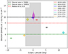 |
Fig. 15. Average electron density, |

Therefore, not only the choice of a time-independent model appears to be less than optimal, but that of a uniform value of ne for pulsars at all ecliptic latitudes in the pulsar timing analysis as well. A better model to describe the SW effects in pulsar timing data is needed to account for an ecliptic-latitude dependency in addition to any temporal variations. Fig. 15 also suggests that the pulsars that populate the low ecliptic latitude regions (the grey shaded area in the plot, highlighting ecliptic latitudes between −3 and 3°) seem to show a systematically higher (and more uniform among different sources)  value with respect to other pulsars. This might be due to a longer exposure to the slow (and denser) phase of the SW during the solar approach. It is important to note that the boundary indicated by the grey shaded region in Fig. 15 does not represent a strict demarcation for the slow wind. In reality, this boundary is determined by the heliographic current sheet (HCS), which does not coincide with the solar equator. During solar maximum, the HCS becomes highly warped (Ballerina skirt-shaped) and inclined relative to the ecliptic plane, resulting in a more complex and oblique solar wind stream, in contrast to the distinct bimodal structure observed during solar minimum (Poletto 2013). Consequently, intermediate scenarios are likely, wherein pulsar’s LoS may pass through different wind streams depending on the tilt of the HCS. Furthermore, this variability can differ between solar activity cycles.
5.3. Temporal variability in ne
From the ne time series in Fig. 12, some pulsars, such as PSRs J2145−0750 and J1744−1134, exhibit a clear correlation with the solar activity cycle, with a peak ne value during the solar maximum (around MJD 56750, April 2014) and minima during the solar minimum (around MJD 58820, December 2019), in what seems to follow a sine wave with an 11-year period. Other pulsars, on the other hand, such as PSRs J1022+1001 and J0030+0451, do not display any notable 11 year periodicity. In general we can note that pulsars with low ecliptic latitudes seem to have relatively constant ne, while sources with medium-to-high ecliptic latitudes tend to show a variability correlated with the solar cycle.
Physically, such behaviour could be induced by how the two SW phases interact during the solar cycle, as shown by the Ulysses mission (McComas et al. 1998). The Ulysses results showed that during the solar minimum the SW has a distinct bimodal distribution with approximately well-defined boundaries, with the slow wind being relatively constrained around the neutral magnetic field line and the fast wind elsewhere. However, during the maximum, these two phases tend to mix at intermediate heliographic latitudes. We stress that heliographic and ecliptic coordinates are two different reference frames, and that the time-dependent neutral magnetic field line is not aligned with the ecliptic. However, the LoS of pulsars with low ecliptic latitudes should mostly pass through the slow wind, especially during the solar approach and egress11.
This may be the reason pulsars at low ecliptic latitudes maintain a more stable, high ne value (due to the presence of a dense SW) throughout the solar cycle. Moreover, pulsars with intermediate-to-high ecliptic latitudes would be sensitive to the ne variability dictated by the solar cycle in this framework, as we expect the LoS to be passing through the fast wind during the periods of solar minima (causing the ne lows that we observe in Fig. 12), and during the solar maxima, the LoS possibly passes through a mixture of fast and slow wind (hence denser than the fast wind alone), causing the highs in ne shown in Fig. 12.
5.3.1. Comparison with the OMNI data
We compared the ne time series of a subset of pulsars with the proton density at 1 AU12 provided by the OMNI database (Papitashvili et al. 2014), as obtained with the in-situ spacecraft solar wind Electron Proton Alpha Monitor (SWEPAM) for the Advanced Composition Explorer (ACE, see McComas et al. 1998) and DISCOVR. In Fig. 16 we report the results of the comparison, for which we only consider those pulsars that satisfy the condition of |ELAT|< 3° since the spacecraft cover the ecliptic region in particular. The black violins represent the probe measurements, with the spread of each violin indicating their range of values in ±2 hours from the time of each pulsar observation, while the red boxes represent the variations in ne values of each pulsar during the solar approach. Pulsar observations provide estimates of the integrated free-electron column density, which are subsequently modelled (as described in Sect. 2.5) to derive a value of ne at 1 AU. In contrast, the OMNI database provides spot measurements of the free proton density at 1 AU. This fundamental difference accounts for many of the discrepancies between the two datasets, highlighting the fact that the modelling efforts applied to the pulsar data are overly simplistic. While such models may be useful for pulsar-timing experiments (Tiburzi et al. 2019), Fig. 16 demonstrates their inadequacy for space-weather studies in their current form.
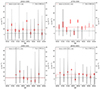 |
Fig. 16. Comparison with in situ Observations: The Fig. shows the variations of ne derived from pulsar observations (red boxes) using the models described in this paper. Only observations where the angular separation between the pulsar and the Sun is less than 30 degrees, as seen from Earth, are included. The red horizontal line represents the median of the pulsar-derived electron density values. The black violin plots indicate the variations in proton density (nP) from the OMNI data, measured within a ±2 hour window around each pulsar observation. The horizontal black dashed line denotes the mean proton density from the OMNI data corresponding to the pulsar observation times. Since the space probes measure proton densities and the pulsars measure electron densities, direct comparison between the two is non-trivial. The four panels represent different pulsars: J1022+1001, J1730-2304, J1400-1431, and J0030+0451, each showing unique density variations over time. |
The differences between the pulsar-derived electron densities and the in situ spacecraft measurements of proton densities indicate that our pulsar modelling efforts (which adhere to industry standards used in pulsar timing experiments, e.g., Antoniadis et al. 2023b) are insufficient for accurately modelling space weather. However, pulsar measurements of loS integrals through the solar wind offer a unique, high-precision contribution to space weather studies by providing meaningful additional constraints to any solar-wind models across multiple lines of sight, at various ecliptic latitudes, and across a range of ecliptic longitudes. Incorporating such measurements into space-weather models is bound to be complex and challenging, but it holds significant promise.
5.3.2. Sensitivity to the solar activity cycle
In Fig. 17 we isolated the ne values of the pulsars with higher ecliptic latitudes, particularly PSRs J2145−0750 and J1744−1134. These pulsars display a clear sensitivity to the activity cycle with consistently low values for ne during solar minima (likely because the LoS is dominated by the fast wind at those times). In contrast, during solar maxima the LoS of these pulsars may experience various degrees of mixing of the fast and slow winds, leading to different, but generally higher values for ne.
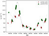 |
Fig. 17. Values of ne obtained from pulsars away from the ecliptic. We discarded PSRs J0034−0534 and J2256−1024 from this plot as both of them were categorised special cases. |
5.4. Two special cases: PSRs J0034−0534 and J2256−1024
PSR J0034−0534 is observed by the LOFAR Core and the GLOW stations as part of various pulsar monitoring projects. This pulsar has the highest DM precision among the MSPs in the LOFAR sample (see Donner et al. 2020), with a median DM uncertainty of ∼2.64 × 10⁻⁵ pc cm−3. The DM time series of this pulsar is shown in Fig. 18 using the Epoch-wise method.
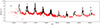 |
Fig. 18. Time series of DM variations for PSR J0034−0534. The black points are the epochs at which the pulsar is closest to the Sun with a solar angle less than 45°. The red points are further away from the Sun. |
The DM precision is such that the solar wind signal remains noticeable in the data even beyond a solar angle of 45° and that our measurements have significant level of sensitivity to the asymmetry in the DM values around the solar conjunction (also pointed out in Tiburzi et al. 2019). As a result, attempts to incorporate higher-order variations in ne for this pulsar have resulted in nonphysical models, particularly during anti-solar conjunctions. After verifying that these issues were unaffected by the modelling of the other noise processes, we therefore concluded that the best way forward for this pulsar was to constrain the SWGP model to only describe the long-term variability associated with the solar cycle and to leave the higher order variations in the solar wind to be modelled by DMGP. Ideally, a more complex solar wind model would be used, which could adequately describe the non-spherical nature of the solar wind; however such a development is beyond the scope of this paper. Hence, we limited the cutoff frequency to 1/(10 yr), which corresponds to 1/tspan. One consequence of this simplistic SWGP model for this pulsar is that our ne values are systematically offset from those reported by Tiburzi et al. (2021), as this offset is absorbed in the model for the IISM contribution. Specifically, we posit that the analysis by Tiburzi et al. (2021) erroneously ascribed significant interstellar dispersion variations as arising from the solar wind, while our analysis avoids such leakage.
PSR J2256−1024 also exhibits a complicated scenario. In particular, it has the shortest time span of our sample (see Fig. 11) and the DM reconstruction via laforge shows a number of epochs with negative values, which is non-physical. Unlike PSR J0034−0534, we suspect this might be due to correlation between the variability in the SW electron density and variations in the interstellar DM. We observe that whenever the DM noise is absorbing some SW noise, particularly at the solar conjunction, SWGP attempts to compensate for that absorption with negative peaks. This covariance with DMGP is an inherent flaw of this model that will have to be taken into account in future analyses.
6. Application of SWGP as a common signal on real data
The previous section showed the occurrence of a bi-modality in the ne behaviour for the pulsars in our sample:
Pulsars with low ecliptic latitude (between −3 and 3 degrees):
-
High values for mean ne;
-
No clear temporal evolution in ne;
Pulsars with medium-to-high ecliptic latitude (from −20 to −3 degrees and from 3 to 20 degrees):
-
Low values of mean ne;
-
The temporal pattern of ne is correlated with the solar cycle.
This outcome shows that we cannot consider the SW as a common signal among all the pulsars in the sample, however, it seems that it might be regarded as such within these two groups separately. Therefore, we repeated our analysis by configuring the enterprise model to apply the SWGP noise component in common among the pulsars of the first group (encompassing PSRs J0030+0451, J1022+1001, J1400−1431, and J1730−2304) and among the pulsars of the second group (all the other sources minus PSR J0034−0534), while maintaining the original settings established in the single-pulsar noise analysis for the other noise elements.
6.1. Common signal for pulsars with low ecliptic latitudes
Fig. 19 illustrates the posterior distribution of the time-varying component for pulsars with an ecliptic latitude between −3° and 3°. The red histogram in the corner plot depicts the parameters corresponding to the common signal. The same parameters derived individually for each pulsar (as obtained from the analysis in the previous section and represented by different colours) agree well with the outcomes derived from the common noise model. Additionally, the common noise exhibits narrower constraint compared to the ones obtained for the individual pulsars, hence, supporting its more optimal performance. PSR J1730−2304 (depicted in green in Fig. 19) displays the broadest posterior distribution, likely due to insufficient observing cadence during the solar conjunctions.
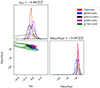 |
Fig. 19. Posterior distributions for the spectral parameters from the SWGP analysis, modelling the time variability as a common signal (red) between all pulsars within three degrees of the ecliptic plane; or separately for each pulsar individually (blue, black, purple and green). The titles shown depict the median values for the common noise part corresponding to the red histogram. |
6.2. Common signal for pulsars with medium-to-high ecliptic latitudes
Fig. 20 displays the posterior distributions for the pulsars in our sample situated the furthest away from the ecliptic region. Once again, the red histogram represents the posteriors for the common SW signal. These distributions indicate that the amplitude of SWGP here is higher when compared to the previous case described in Sect. 6.1, possibly suggesting a greater variability. However, there are clear discrepancies between the parameters of the common signal and the ones derived for the individual pulsars.
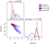 |
Fig. 20. Posterior distributions for the spectral parameters from the SWGP analysis, modelling time variability as a common signal (red) between all pulsars beyond three degrees from the ecliptic plane, or separately for each pulsar individually (blue, black, purple). The titles shown depict the median values for the common noise part corresponding to red histogram. |
In particular, PSR J1744−1134 deviates the most from both the other pulsars and the common noise parameters, indicating pulsar-specific variability in amplitude and slope. This deviation can be attributed to PSR J1744−1134’s ecliptic latitude of 11.81°, namely, the farthest from the Sun among the pulsars in our study.
PSRs J2145−0750 and J2256−1024 are more consistent with the parameters of the common signal within the uncertainty ranges, although not as prominently as in the previous scenario. This experiment underlines the need for caution when considering a common SW signal for pulsars located away from the ecliptic, as their variability seems to imply the necessity for individual treatment.
7. Conclusions
In this study, we applied and tested SWGP, a Bayesian, Gaussian-process approach to model the time-variable solar wind signal in pulsar-timing data, which approximates the power spectrum of its temporal density variations with a power law; with its spatial electron-density distribution as being spherical. The resulting data products from the application of SWGP are the posterior distribution of both the amplitude and spectral index of the power spectrum; from these, we reconstructed the time series of both the corresponding amplitudes of the spherical SW model at 1 AU, ne, and of the corresponding DM time series, using the laforge software package.
First, we validated the method against pulsar-timing simulations with a progressively increasing level of complexity. The model performed well against all the simulations, including the ones that do not rely on a spherical distribution of free electrons for the SW (see Sect. 3.3). We then applied the SWGP module alongside the other commonly used noise components in pulsar-timing noise analysis to study the SW trends in a sample of millisecond pulsars observed for about ten years with the low-frequency interferometer LOFAR. The analysed observations are particularly sensitive to plasma-related propagation effects. Our results highlight important implications for pulsar timing and related noise analyses, which can be summarised as follows:
-
The ne parameter affecting pulsar observations is both dependent on the time of the observation and the ecliptic latitude of the pulsars concerned, in contrast to the assumptions typically used in pulsar timing analyses. This also places an emphasis on the viability of spherical model to account for the effects of SW which does not fully explain the intricacies of this noise process.
-
Pulsars with low ecliptic latitude (within three degrees of the plane) have systematically higher values of
 than pulsars with medium-to-high ecliptic latitudes (between three and 20 degrees from the plane).
 -
The temporal evolution of inferred ne values is different for pulsars at low ecliptic latitudes and for pulsars at medium-to-high ecliptic latitudes.
-
Pulsars with low ecliptic latitude do not show clear ne temporal patterns
-
Pulsars with medium-to-high ecliptic latitude show a quite distinct temporal pattern in ne, that correlates with the solar cycle, with peaks of ne reached during the solar maximum, and dips of ne reached during the minimum.
We also confirmed this difference in behaviour by using SWGP as a common noise model for pulsars with low ecliptic latitude and medium-to-high ecliptic latitude. This exercise showed that while the posteriors of low ecliptic sources tended to agree with the ones of the common signal, for the second group there was less consistency between the common signal and the individual time variability posteriors.
The physical reasons of these features probably lies in the bimodal SW nature, that materialises in a slow-wind phase and a fast-wind phase and in their interaction during the solar cycle. While the verification of this hypothesis is beyond the scope of this article, it may be pursued by evaluating the distribution of slow and fasts solar wind along the LoS for each pulsar observation, for instance, based on white-light images of the solar environment or solar magnetograms, or through the comparison of the LoS positions within the 3D reconstructions of the SW that can be offered by space-weather software such as EUHFORIA or 3D IPS tomography (Tiburzi et al. 2023; Shaifullah et al. 2023). In turn, pulsar observations prove to be optimal bench tests for such software, and might be able to contribute to their functionalities in the near future.
The name of this method comes from its aim to obtain a DM time series by fitting the frequency-resolved timing residuals, rν, i, of each observation, i as:
where Ci is an offset that contains any possible achromatic delay introduced by errors in the timing model, and any unaccounted red noise.
While at the solar conjunction any pulsar that is not occulted by the Sun will hover above or below the solar disk, therefore the LoS at that point will be likely affected mainly by the fast wind
Due to the presence of He+ ions, the proton density is slightly lower than the electron density, but there is no clear consensus on the conversion factor between the two.
Acknowledgments
SCS acknowledges the support of College of Science and Engineering University of Galway Postgraduate Scholarship in supporting this work. ACh and GMS acknowledge financial support provided under the European Union’s H2020 ERC Consolidator Grant “Binary Massive Black Hole Astrophysics” (B Massive, Grant Agreement: 818691). JPWV acknowledges support from NSF AccelNet award No. 2114721. JSH acknowledges support from NSF CAREER award No. 2339728 and NSF Physic Frontiers Center award No. 2020265. FI was supported by the University of Cagliari, Italy and the Istituto Nazionale di Astrofisica (INAF). Pulsar research at Jodrell Bank Centre for Astrophysics is supported by an STFC Consolidated Grant (ST/T000414/1; ST/X001229/1). This paper is based on data obtained with the German stations of the International LOFAR Telescope (ILT), constructed by ASTRON [van Haarlem et al. (2013)], during station-owners time. In this work we made use of data from the Effelsberg (DE601) LOFAR station funded by the Max-Planck-Gesellschaft; the Unterweilenbach (DE602) LOFAR station funded by the Max-Planck-Institut für Astrophysik, Garching; the Tautenburg (DE603) LOFAR station funded by the State of Thuringia, supported by the European Union (EFRE) and the Federal Ministry of Education and Research (BMBF) Verbundforschung project D-LOFAR I (grant 05A08ST1); the Potsdam (DE604) LOFAR station funded by the Leibniz-Institut für Astrophysik, Potsdam; the Jülich (DE605) LOFAR station supported by the BMBF Verbundforschung project D-LOFAR I (grant 05A08LJ1); and the Norderstedt (DE609) LOFAR station funded by the BMBF Verbundforschung project D-LOFAR II (grant 05A11LJ1). The observations of the German LOFAR stations were carried out in the stand-alone GLOW mode (German LOng-Wavelength array), which is technically operated and supported by the Max-Planck-Institut für Radioastronomie, the Forschungszentrum Jülich and Bielefeld University. We acknowledge support and operation of the GLOW network, computing and storage facilities by the FZ-Jülich, the MPIfR and Bielefeld University and financial support from BMBF D-LOFAR III (grant 05A14PBA) and D-LOFAR IV (grant 05A17PBA), and by the states of Nordrhein-Westfalia and Hamburg.
References
- Agazie, G., Archibald, A. M., Arzoumanian, Z., et al. 2023, ApJ, 951, L8 [NASA ADS] [CrossRef] [Google Scholar]
- Alpar, M. A., Nandkumar, R., & Pines, D. 1986, ApJ, 311, 197 [NASA ADS] [CrossRef] [Google Scholar]
- Antoniadis, J., Arumugam, S., Babak, S., et al. 2023a, A&A, 678, A50 [CrossRef] [EDP Sciences] [Google Scholar]
- Antoniadis, J., Bak Nielsen, A.-S., Bassa, C. G., et al. 2023b, A&A, 678, A48 [Google Scholar]
- Arzoumanian, Z., Brazier, A., Burke-Spolaor, S., et al. 2018, ApJS, 235, 37 [CrossRef] [Google Scholar]
- Backer, D. C., Heiles, C., Davis, M. M., et al. 1982, Nature, 300, 615 [NASA ADS] [CrossRef] [Google Scholar]
- Biermann, L. 1951, Z. Astrophys., 29, 274 [NASA ADS] [Google Scholar]
- Bray, J., Roberts, P., Reynolds, J., et al. 2015, Astropart. Phys., 65, 22 [NASA ADS] [CrossRef] [Google Scholar]
- Chalumeau, A., Petiteau, A., Chen, S., et al. 2021, MNRAS, 509, 5538 [NASA ADS] [CrossRef] [Google Scholar]
- Counselman, C., III, & Rankin, J. 1972, ApJ, 175, 843 [NASA ADS] [CrossRef] [Google Scholar]
- Donner, J. Y., Tiburzi, C., Oslowski, S., et al. 2020, A&A, 644, A153 [NASA ADS] [CrossRef] [EDP Sciences] [Google Scholar]
- Edwards, R. T., Hobbs, G. B., & Manchester, R. N. 2006, MNRAS, 372, 1549 [Google Scholar]
- Ellis, J. A., Vallisneri, M., Taylor, S. R., & Baker, P. T. 2019, ENTERPRISE: Enhanced Numerical Toolbox Enabling a Robust PulsaR Inference SuitE, Astrophysics Source Code Library [record ascl:1912.015] [Google Scholar]
- EPTA Collaboration (Antoniadis, J., et al.) 2023, A&A, 678, A49 [Google Scholar]
- Feldman, U., Schühle, U., Widing, K. G., & Laming, J. M. 1998, ApJ, 505, 999 [Google Scholar]
- Goncharov, B., Shannon, R. M., Zhu, X.-J., et al. 2020, MNRAS, 502, 478 [Google Scholar]
- Guhathakurta, M., & Fisher, R. 1998, ApJ, 499, L215 [Google Scholar]
- Hazboun, J. S. 2020, https://doi.org/10.5281/zenodo.4152550 [Google Scholar]
- Hazboun, J. S., Taylor, S. R., Lam, M. T., et al. 2020, ApJ, 890, 108 [NASA ADS] [CrossRef] [Google Scholar]
- Hazboun, J., Simon, J., Madison, D. R., et al. 2022, ApJ, 929, 39 [NASA ADS] [CrossRef] [Google Scholar]
- Hellings, R. W., & Downs, G. S. 1983, ApJ, 265, L39 [NASA ADS] [CrossRef] [Google Scholar]
- Hobbs, G. B., Edwards, R. T., & Manchester, R. N. 2006a, MNRAS, 369, 655 [Google Scholar]
- Hobbs, G., Lyne, A., & Kramer, M. 2006b, Chin. J. Astron. Astrophys. Suppl., 6, 169 [NASA ADS] [CrossRef] [Google Scholar]
- Hotan, A. W., van Straten, W., & Manchester, R. N. 2004, PASA, 21, 302 [Google Scholar]
- Issautier, K., Moncuquet, M., & Hoang, S. 2003, AIP Conf. Proc., 679, 59 [NASA ADS] [CrossRef] [Google Scholar]
- Keith, M. J., Shannon, R. M., Hobbs, G. B., et al. 2013, MNRAS, 429, 2161 [NASA ADS] [CrossRef] [Google Scholar]
- Kulkarni, S. R. 2020, ArXiv e-prints [arXiv:2007.02886] [Google Scholar]
- Kumar, P., Stovall, K., Dowell, J., et al. 2022, MNRAS, 511, 3937 [NASA ADS] [CrossRef] [Google Scholar]
- Lazarus, P., Graikou, E., Caballero, R. N., et al. 2016, MNRAS, 458, 868 [NASA ADS] [CrossRef] [Google Scholar]
- Liu, K., Lee, K. J., Kramer, M., et al. 2012, MNRAS, 420, 361 [NASA ADS] [CrossRef] [Google Scholar]
- Lorimer, D. R., & Kramer, M. 2004, Handbook of Pulsar Astronomy (Cambridge, UK: Cambridge University Press), 4 [Google Scholar]
- Madison, D. R., Cordes, J. M., Arzoumanian, Z., et al. 2019, ApJ, 872, 150 [Google Scholar]
- Marsden, R. G., & Wenzel, K. P. 1991, ESA Bull., 67, 78 [NASA ADS] [Google Scholar]
- McComas, D. J., Barker, P., Feldman, W. C., et al. 1998, Space Sci. Rev., 86, 563 [CrossRef] [Google Scholar]
- Melatos, A., & Link, B. 2013, MNRAS, 437, 21 [Google Scholar]
- Muhleman, D. O., & Anderson, J. D. 1981, ApJ, 247, 1093 [Google Scholar]
- Nitu, I. C., Tiburzi, C., Brüggen, M., et al. 2024, MNRAS, 528, 3304 [NASA ADS] [CrossRef] [Google Scholar]
- Papitashvili, N., Bilitza, D., & King, J. 2014, in 40th COSPAR Scientific Assembly, 40, C0.1-12-14 [Google Scholar]
- Poletto, G. 2013, J. Adv. Res., 4, 215 [NASA ADS] [CrossRef] [Google Scholar]
- Rasmussen, C. E., & Williams, C. K. I. 2006, Gaussian Processes for Machine Learning [Google Scholar]
- Reardon, D. J., Shannon, R. M., Hobbs, G. B., et al. 2023, ApJ, 951, L6 [NASA ADS] [CrossRef] [Google Scholar]
- Shaifullah, G. M., Tiburzi, C., Jebaraj, I., et al. 2023, Adv. Space Res., 72, 5298 [NASA ADS] [CrossRef] [Google Scholar]
- Swiggum, J., & NANOGrav Pfc 2022, Am. Astron. Soc. Meeting Abstr., 54, 348.08 [Google Scholar]
- Tarafdar, P., Rana, P., Singha, J., et al. 2022, PASA, 39, e053 [NASA ADS] [CrossRef] [Google Scholar]
- Taylor, S. R., Hazboun, J. S., Simon, J., et al. 2021, enterprise_extensions, v2.3.3 [Google Scholar]
- Tiburzi, C., Kerr, M., Coles, W. A., et al. 2015, MNRAS, 455, 4339 [Google Scholar]
- Tiburzi, C., Shaifullah, G. M., Janssen, G. H., et al. 2019, MNRAS, 487, 394 [NASA ADS] [CrossRef] [Google Scholar]
- Tiburzi, C., Bassa, C. G., Zucca, P., et al. 2021, A&A, 647, A84 [NASA ADS] [CrossRef] [EDP Sciences] [Google Scholar]
- Tiburzi, C., Cota, L., Shaifullah, G. M., et al. 2023, Adv. Space Res., 72, 5287 [NASA ADS] [CrossRef] [Google Scholar]
- Tokumaru, M., Takefuji, K., Sekido, M., et al. 2020, Sol. Phys., 295, 80 [NASA ADS] [CrossRef] [Google Scholar]
- van Haarlem, M. P., Gunst, A. W., Heald, G., et al. 2013, A&A, 556, A2 [NASA ADS] [CrossRef] [EDP Sciences] [Google Scholar]
- Van Haasteren, R., & Vallisneri, M. 2014, Phys. Rev. D, 90, 10 [CrossRef] [Google Scholar]
- van Haasteren, R., Levin, Y., McDonald, P., & Lu, T. 2009, MNRAS, 395, 1005 [NASA ADS] [CrossRef] [Google Scholar]
- van Straten, W., & Bailes, M. 2011, PASA, 28, 1 [Google Scholar]
- van Straten, W., Khoo, J., Keith, M., et al. 2011, PSRCHIVE: Development Library for the Analysis of Pulsar Astronomical Data, Astrophysics Source Code Library [record ascl:1105.014] [Google Scholar]
- Wang, Y. 2015, J. Phys.: Conf. Ser., 610, 012019 [NASA ADS] [CrossRef] [Google Scholar]
- You, X. P., Coles, W. A., Manchester, R. N., et al. 2007a, MNRAS, 378, 493 [NASA ADS] [CrossRef] [Google Scholar]
- You, X. P., Coles, W. A., Manchester, R. N., et al. 2007b, ApJ, 671, 907 [NASA ADS] [CrossRef] [Google Scholar]
- Zic, A., Reardon, D. J., Kapur, A., et al. 2023, PASA, 40, e049 [NASA ADS] [CrossRef] [Google Scholar]
All Tables
Parameters of the noise components injected in scenario 2 of the first test case.
Parameters of the noise components injected in the simulations that assume a continuously varying ne value.
All Figures
|
Fig. 1. Sample results from one SWGP realisation. In a hypothetical scenario, considering the long time span of one of the pulsars in our dataset PSR J1022+1001. The top panel shows the variations in ne that can be modelled using SWGP perturbed from the mean value. The middle panel shows the corresponding time delays due to SWGP. The bottom panel shows the time delay when the deterministic signal with an |
| In the text | |
|
Fig. 2. Simulation scenario 1, only SW. Top: ne variations simulated (blue) are shown as well as the mean value (red) and the ne retrieved (green) when fit for a single value with TEMPO2. Middle: Blue points represent the residuals corresponding to the injected values of ne. Bottom: Green points represent the residuals after a constant |
| In the text | |
|
Fig. 3. Simulation scenario 2, with noise. Posterior chain plot for yearly varying ne scenario. The black lines represent the truth values injected into the simulations. The black line in |
| In the text | |
|
Fig. 4. Time domain reconstruction of the inserted simulations with various noise parameters embedded into it. It presents the specified noise parameters as in Table 2 along with the SW signal. The blue points are the simulated residuals and the orange lines are the recovery after the noise analysis. |
| In the text | |
|
Fig. 5. ne plotted as a function of MJD for continuously varying SW scenario. |
| In the text | |
|
Fig. 6. Time domain reconstruction from the continuously varying SW scenario. |
| In the text | |
|
Fig. 7. DM time series for replicating the solar activity in ne. The blue points are injected ones, while the red points with the error bars are recovered from the noise analysis run after modelling using SWGP. |
| In the text | |
|
Fig. 8. ne recovered from the recovered DM time series in Fig. 7. The orange sine curve is the ne injected into the simulations mimicking the solar activity cycle. The black dotted line represented the average of all injected ne. |
| In the text | |
|
Fig. 9. Time domain reconstruction from the simulations when the two-phase model was used. These simulations have WN and the SW noise. |
| In the text | |
|
Fig. 10. Locations of the pulsar in reference to the Sun in equatorial coordinates. The yellow line represents the path of the Sun and the coloured dots represent the locations of each pulsar. |
| In the text | |
|
Fig. 11. DM time−series obtained from the changing SWGP+deterministic ne part of the posterior chain. The black points correspond to epochs with |solar_angle|< 45° from the Sun and the vertical dashed lines indicate a solar conjunction. The order of the pulsars is aligned according to their distance from the Sun in terms ecliptic latitude in ascending order. |
| In the text | |
|
Fig. 12. Values of ne extracted from the DM time series shown in Fig. 11. The black points represent the epochs that have |solar_angle|< 45°. The blue points are obtained from the results presented in Tiburzi et al. (2021). The order of the pulsars is aligned according to their distance from the Sun in terms ecliptic latitude in ascending order. The long term solar cycle is evident in pulsars more than 3° away from the Sun in terms of ecliptic latitude i.e. the bottom four panels. |
| In the text | |
|
Fig. 13. DM time series for PSR J2145−0750 obtained with different noise elements. Top panel shows the DM reconstruction from the SWGP model. The second panel demonstrates the result from the |
| In the text | |
|
Fig. 14. Demonstration of SWGP model in comparison with the Epoch-wise method as a function of solar angle on PSR J2145−0750. Here, we consider the binned average over 1° of solar angle. This elucidates the working of SWGP particularly for epochs less than 30° from the Sun. |
| In the text | |
|
Fig. 15. Average electron density, |
| In the text | |
|
Fig. 16. Comparison with in situ Observations: The Fig. shows the variations of ne derived from pulsar observations (red boxes) using the models described in this paper. Only observations where the angular separation between the pulsar and the Sun is less than 30 degrees, as seen from Earth, are included. The red horizontal line represents the median of the pulsar-derived electron density values. The black violin plots indicate the variations in proton density (nP) from the OMNI data, measured within a ±2 hour window around each pulsar observation. The horizontal black dashed line denotes the mean proton density from the OMNI data corresponding to the pulsar observation times. Since the space probes measure proton densities and the pulsars measure electron densities, direct comparison between the two is non-trivial. The four panels represent different pulsars: J1022+1001, J1730-2304, J1400-1431, and J0030+0451, each showing unique density variations over time. |
| In the text | |
|
Fig. 17. Values of ne obtained from pulsars away from the ecliptic. We discarded PSRs J0034−0534 and J2256−1024 from this plot as both of them were categorised special cases. |
| In the text | |
|
Fig. 18. Time series of DM variations for PSR J0034−0534. The black points are the epochs at which the pulsar is closest to the Sun with a solar angle less than 45°. The red points are further away from the Sun. |
| In the text | |
|
Fig. 19. Posterior distributions for the spectral parameters from the SWGP analysis, modelling the time variability as a common signal (red) between all pulsars within three degrees of the ecliptic plane; or separately for each pulsar individually (blue, black, purple and green). The titles shown depict the median values for the common noise part corresponding to the red histogram. |
| In the text | |
|
Fig. 20. Posterior distributions for the spectral parameters from the SWGP analysis, modelling time variability as a common signal (red) between all pulsars beyond three degrees from the ecliptic plane, or separately for each pulsar individually (blue, black, purple). The titles shown depict the median values for the common noise part corresponding to red histogram. |
| In the text | |
Current usage metrics show cumulative count of Article Views (full-text article views including HTML views, PDF and ePub downloads, according to the available data) and Abstracts Views on Vision4Press platform.
Data correspond to usage on the plateform after 2015. The current usage metrics is available 48-96 hours after online publication and is updated daily on week days.
Initial download of the metrics may take a while.