| Issue |
A&A
Volume 692, December 2024
|
|
|---|---|---|
| Article Number | A170 | |
| Number of page(s) | 15 | |
| Section | Numerical methods and codes | |
| DOI | https://doi.org/10.1051/0004-6361/202450740 | |
| Published online | 13 December 2024 | |
Pulsar timing methods for evaluating dispersion measure time series
1
INAF – Osservatorio Astronomico di Cagliari,
via della Scienza 5,
09047
Selargius (CA),
Italy
2
Dipartimento di Fisica, Università di Cagliari, Cittadella Universitaria,
09042
Monserrato (CA),
Italy
3
Dipartimento di Fisica “G. Occhialini”, Università degli Studi di Milano-Bicocca,
Piazza della Scienza 3,
20126
Milano,
Italy
4
INFN, Sezione di Milano-Bicocca,
Piazza della Scienza 3,
20126
Milano,
Italy
5
Florida Space Institute, University of Central Florida,
12354 Research Parkway,
Orlando,
FL
32826,
USA
6
Physics, School of Natural Sciences, Ollscoil na Gaillimhe – University of Galway,
University Road,
Galway,
H91 TK33,
Ireland
7
Max-Planck-Institut für Radioastronomie,
Auf dem Hügel 69,
53121
Bonn,
Germany
8
Fakultät für Physik, Universität Bielefeld,
Postfach 100131,
33501
Bielefeld,
Germany
9
National Centre for Radio Astrophysics,
Pune University Campus,
Pune
411007,
India
10
SETI Institute,
339 N Bernardo Ave Suite 200,
Mountain View,
CA
94043,
USA
11
School of Physics and Astronomy, Rochester Institute of Technology,
Rochester,
NY
14623,
USA
12
Laboratory for Multiwavelength Astrophysics, Rochester Institute of Technology,
Rochester,
NY
14623,
USA
13
National Research Council Postdoctoral Associate, National Academy of Sciences,
Washington,
DC
20001,
USA resident at
Naval Research Laboratory,
Washington,
DC
20375,
USA
14
Space Science Division, Naval Research Laboratory,
Washington,
DC
20375–5352,
USA
15
LPC2E – Université d’Orléans / CNRS,
45071
Orléans cedex 2,
France
16
Observatoire Radioastronomique de Nançay (ORN), Observatoire de Paris, Université PSL, Univ Orléans, CNRS,
18330
Nançay,
France
★ Corresponding author; This email address is being protected from spambots. You need JavaScript enabled to view it.
Received:
16
May
2024
Accepted:
19
October
2024
Abstract
Context. Radio pulsars can be used for many studies, including the investigation of the ionized interstellar medium and the solar wind via their dispersive effects. These phenomena affect the high-precision timing of pulsars and are among the main sources of noise in experiments searching for low-frequency gravitational waves in pulsar data.
Aims. In this paper, we compare the functionality and reliability of three commonly used schemes to measure temporal variations in interstellar propagation effects in pulsar timing data.
Methods. We carried out extensive simulations at low observing frequencies (100–200 MHz) by injecting long-term correlated noise processes with power-law spectra and white noise, to evaluate the robustness, accuracy, and precision of the following three mitigation methods: epoch-wise (EW) measurements of interstellar dispersion; the DMX method of simultaneous, piece-wise fits to interstellar dispersion; and DM GP, which models dispersion variations through Gaussian processes using a Bayesian analysis method. We then evaluated how reliably the input signals were reconstructed and how the various methods reacted to the presence of achromatic long-period noise.
Results. All the methods perform well, provided the achromatic long-period noise is modeled for DMX and DM GP. The most precise method is DM GP, followed by DMX and EW, while the most accurate is EW, followed by DMX and DM GP. We also tested different scenarios including simulations of L-band times of arrival and realistic DM injection, with no significant variation in the obtained results.
Conclusions. Given the nature of our simulations and our scope, we deem that EW is the most reliable method to study the Galactic ionized media. Follow-up works should be conducted to confirm this result via more realistic simulations. We note that DM GP and DMX seem to be the best-performing techniques in removing long-term correlated noise, and hence for gravitational wave studies. However, full simulations of pulsar timing array experiments are needed to support this interpretation.
Key words: methods: data analysis / pulsars: general
© The Authors 2024
 Open Access article, published by EDP Sciences, under the terms of the Creative Commons Attribution License (https://creativecommons.org/licenses/by/4.0), which permits unrestricted use, distribution, and reproduction in any medium, provided the original work is properly cited.
This article is published in open access under the Subscribe to Open model. This email address is being protected from spambots. You need JavaScript enabled to view it. to support open access publication.
1 Introduction
Pulsars are highly magnetized, rapidly rotating neutron stars that emit beams of radiation, mainly in the radio band, from their magnetic poles. Therefore, pulsars are visible as periodic sources to terrestrial observers. The extremely regular rotation of a pulsar allows one to predict the time of arrival (ToA) of its radiation at a radio observatory and to extract from these data information about the pulsar itself, its environment, and perturbing effects through the pulsar timing procedure (e.g., Lorimer & Kramer 2005). The model that contains the parameters necessary to describe the signal propagation, usually referred to as the timing model, is used to calculate expected ToAs, which are then compared with observed ones to create and analyze the timing residuals (the difference between the observed ToAs and the ones predicted by the timing model). The parameters in the timing model are iteratively fit to minimize the timing residuals and to achieve a more and more precise description of the analyzed pulsars. The shorter the spin period and the brighter the pulsar, the smaller its weighted root-mean-square (RMS) timing residuals and the more precisely determined the timing-model parameters. The most rapidly rotating pulsars are known as “millisecond pulsars” (Backer et al. 1982) because they have spin periods on the order of milliseconds. The technique of pulsar timing opens up the study not only of the physical characteristics of pulsars, but also other effects, such as propagation effects through ionized media (Rickett 1990; Foster & Cordes 1990), the most conspicuous of which is dispersion.
Dispersion is a phenomenon caused by the dependency of a medium’s refractive index, µ, on the frequency, ν, of the propagating radiation and on its own free-electron density, ne. In particular:
 (1)
(1)
with fp, the plasma frequency, defined as
 (2)
(2)
where e and me are, respectively, the electron electric charge and mass. The net effect of these two dependencies is an absolute delay in the arrival time of the radiation bundle after propagating through an ionized medium (such as the interstellar medium, which hosts an ionized component, or the solar wind), and a relative delay among the radiation at different frequencies within that bundle. In particular, we can write the delay, ∆t, for radiation with a frequency ν ≪ fp as:
 (3)
(3)
where 𝔇 is the dispersion constant (Lorimer & Kramer 2005), and the DM parameter is the dispersion measure, defined as
 (4)
(4)
where the integral is performed along the line of sight (LoS) and the units are pc cm−3. The dispersion measure (DM) of a pulsar is one of the parameters included in its timing model.
Equation (3) can be rewritten following (Verbiest & Shaifullah 2018)
 (5)
(5)
where B is the fractional bandwidth, (ν2 − ν1)/νc, and νc is the central frequency of the observing band.
From these equations, it is easy to infer that (i) the DM is a direct measure of the free-electron content along a given LoS and (ii) large delays between radiation emitted at different frequencies of the same bundle are shown over low central observing frequencies and/or large fractional bandwidths. We note that, in practice, an absolute value of DM can never be achieved due to the evolution of pulsar profiles with the observing frequency (e.g., Hassall et al. 2012). To complicate matters further, pulsars are high-velocity objects, following the kick that they receive during the supernova event (Hobbs et al. 2005). This implies that they move rapidly across the sky, and hence the LoS varies significantly as well. In doing so, different parts of the ionized interstellar medium (IISM) are crossed, with different associated values for ne, and hence the value of DM changes with time (Lam et al. 2016). This is why simple polynomial models of DM time evolution are often included in the timing model. Nevertheless, the turbulence in the IISM cannot be correctly described via derivatives only, and hence there are a large number of studies in the literature reporting on the time series of DM variations and their connection with the physics of plasma in the Galaxy.
Recently, Donner et al. (2020) reported the DM variations for 36 millisecond pulsars observed for about 7 years at low radio frequency (100–200 MHz) with the LOFAR (LOw Frequency ARray; see van Haarlem et al. 2013) interferometer, achieving a very low median DM uncertainty on the order of 10−5 pc/cm3 for a significant fraction of the sample. Besides, DM variations were detected when the median DM uncertainty was lower than a few in 10−4 pc/cm3. Krishnakumar et al. (2021) have presented the 1-year long DM time series of four millisecond pulsars observed with uGMRT using BAND3 (400–500 MHz) and BAND5 (1360–1460 MHz). They show that the DM precision improves up to 10−4 pc/cm3 when combining data from both of the bands. Agazie et al. (2023) and Jones et al. (2017) reported on the DM variations of up to 68 millisecond pulsars with mainly the Green Bank (722–1885 MHz) and the Arecibo (302–2400 MHz) radio telescopes, highlighting their monotonic trends and the presence of annual IISM signatures for almost 20 of them. Lastly, Keith et al. (2024) calculated the DM time series for almost 600 long-period pulsars observed with the MeerKAT telescope in the L band (896–1671 MHz) and a large fractional bandwidth, reporting a broad linear correlation between the DM and its first derivative.
While DM variations allow for the investigation of Galactic plasma, when they are unaccounted for they may become a nuisance in other experiments, such as pulsar timing arrays (PTAs; Tiburzi 2018; Verbiest et al. 2021; Taylor 2021) that search for low-frequency gravitational waves (GWs; Maggiore 2018) in pulsar data. In particular, GWs are expected to cause long-term, space- and time-correlated perturbations in pulsar timing residuals, usually characterized by a steep, red power spectrum (Phinney 2001). The PTAs search for these effects by cross-correlating the timing residuals of pairs of selected pulsars, to identify the predicted signature following the so-called Hellings and Downs curve in the case of an isotropic GW background (Hellings & Downs 1983). One of the most challenging parts of PTA analyses is the characterization of signals that are not GWs but that also induce long-term, time-correlated structures in the timing residuals (see, e.g., Verbiest & Shaifullah 2018); in other words, that are sources of red noise (RN). The red-noise processes with the highest amplitudes have two main contributions. The first is often called timing noise, or spin noise, and refers to rotational instabilities of the targeted pulsar (Hobbs et al. 2004). The second is the aforementioned time variability in the amount of interstellar dispersion affecting the pulsar radiation (hereafter referred to as DM noise). The PTAs have historically been focused on high-frequency bands (~1 – 3 GHz), small fractional bandwidths, and/or asynchronous timing observations at different frequency bands (see Lam et al. 2015, where they demonstrated that multi-frequency asynchronous observations will never reduce the timing error due to DM noise below 10 ns). Therefore, while the DM noise does indeed have an impact on the GW search, PTA data have a poor sensitivity toward it (see also Fig. 6 in Verbiest & Shaifullah 2018). This is why PTAs are starting to use observing campaigns obtained with low-frequency, large-bandwidth facilities such as LOFAR and NenuFAR (the New Extension in Nançay Upgrading LOFAR; see Zarka et al. 2012; Donner et al. 2020; Tiburzi et al. 2021; Bondonneau et al. 2021).
In this paper, we aim to assess the performances in terms of precision and accuracy of three methods of calculating DM variations that have been used to study Galactic plasma or to model the DM noise impact in PTA data, based on a comprehensive series of simulations. In Sect. 2, we describe these three approaches and the simulations. In Sect. 3, we report the simulation results, which are discussed in Sect. 4. Finally, in Sect. 5 we draw our conclusions.
We do not assess the impact of GWs on the DM recovery methods; nor do we check the impact of these schemes on the timing model parameters. These aspects will be tested in future works.
We stress that there are also other effects that might affect pulsar timing at low radio frequencies. With LOFAR observations, the ToAs are generated using a frequency-resolved template (see, e.g., Donner et al. 2020; Tiburzi et al. 2021), and hence interstellar scintillation does not affect the timing solution. Pulse broadening and scattering variations are two other features that might be present in low-frequency observations. In this paper, we do not take into account these effects and we simulate a more commonly occurring scenario, without frequency-dependent contributions other than DM variations.
2 Simulations and methods for the analysis
2.1 Simulations
To compare the effectiveness of the various PTA methods of calculating and accounting for DM variations, we evaluated their application to simulated data, which were produced using the libstempo software package (Vallisneri 2020).
2.1.1 Simulations with libstempo
libstempo is a Python wrapper of the TEMPO2 software package (Edwards et al. 2006) that allows the use of all of the TEMPO2 functionalities within a Python-based environment. In particular, we exploited the libstempo.toasim.fake_pulsar library to simulate 10 narrow-band ToAs per observing epoch in the most commonly used LOFAR frequency band for pulsar observations, between 100 and 200 MHz, with 5 µs fixed ToA template-fitting error bars. The simulated observing epochs have a regular fortnightly cadence and cover a time span of Tspan = 3000 days. To build simulations as close as possible to the typical PTA dataset, we injected stochastic noise in the form of white noise (WN), achromatic (i.e., radio-frequency-independent) RN, and DM variations.
The WN reflects instrumental errors and instrumental sensitivity, as well as intrinsic pulse jitter. We modeled it by considering two parameters: EFAC, which is a multiplicative factor that takes into account ToA measurement errors; and EQUAD, which is added in quadrature and accounts for any other WN that may be given by profile variations and possible systematic errors. The final ToA uncertainty is then
 (6)
(6)
where σtemp is the template-fitting error, and it was given as an input to our simulations1.
Achromatic RN, and DM variations, are both time-correlated noise processes that are modeled with a Fourier basis of Nf coefficients and a power-law power spectrum (EPTA Collaboration & InPTA Collaboration 2023). We distinguished between chromatic and achromatic noise processes using a chromatic index, α, equal, respectively, to 2 and 0. The time delay induced on a ToA with frequency, ν, at an epoch, t, is then:
 (7)
(7)
𝒫i· is the power-law power spectral density with hyperparameters Â, the normalized amplitude at the frequency of 1 yr−1, and γ, the spectral index. It is written as follows:
 (8)
(8)
with n = RN or DM, and we refer to the amplitude as An = log10(Ân). F is the matrix of the cosine functions at each Fourier frequency, fi = i/Nf, and time, t:
 (9)
(9)
with ϕ being a random phase drawn from 𝒰(0, 2π). The radio frequency is ν and the reference frequency, νref, was set to 1.4 GHz. The time series of the injected noise signal is then a sum over a finite number, Nf, of cosine functions (see the second and third rows of Fig. 1 for an example). For both RN and DM noise, we considered Nf = 30 components. This corresponds to a frequency of about 1.15 × 10⁻⁷ Hz, which is close to the Nyquist one that, given our 14 days of cadence, is at around 2 × 10⁻⁷ Hz.
2.1.2 Simulation parameters
Table 1 shows all the parameters adopted for our simulations, with σtemp, EFAC, and EQUAD being fixed, respectively, to 5 µs, 1.2, and 2 µs for all the cases. Concerning the noise spectral indices, we first assumed a realistic spectral index for DM variations from the Kolmogorov turbulence theory (Armstrong et al. 1995) (γDM = 8/3) and a steeper one for the RN (γRN = 3.7). Secondly, we considered a different pair of spectral indices: γDM = 3.2 and γRN = 2.5. For each pair of spectral indices, we have studied three fixed values of amplitude of the power spectrum for both of the noise processes, producing a total of nine datasets per pair of spectral indices. ARN and ADM have been chosen within the range of values reported by EPTA Collaboration & InPTA Collaboration (2023).
For each specific set of ARN and ADM and pair of spectral indices, we generated a total of 100 timing residuals realizations. In each realization, the seed for the injected RN was kept constant to maintain the same RN signature across all timing residuals, while the DM noise seed varies with each iteration, resulting in distinct DM time series for all 100 realizations.
Figure 1 clarifies our simulation process by reporting three different scenarios, each of them with a different ADM that increases going from left to right. The first row reports the overall timing residuals; the second row shows the delay due to the injected RN; and the third row illustrates the DM variations introduced in our dataset. The last row represents the power spectrum of the noise processes involved in the three scenarios. We note that the first and third rows of each column each report only 1 of the 100 realizations that have been created for that set of parameters.
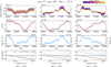 |
Fig. 1 Simulations carried out with injected values of γRN, ARN, and γDM of, respectively, 3.7, −13.3, and 8/3. The columns are associated with increasing values of ADM, left to right (as is indicated at the bottom). First row: 1 out of the 100 simulated timing residuals with a color map associated with the observing frequency (as is reported in the top right corner). Second row: injected RN signal. Third row: 1 out of the 100 different injections of the DM time series. On the right y axis, we report the corresponding time delay at the reference frequency of 150 MHz. Fourth row: Power spectra of the injected noise processes; WN (black), RN (red), and DM variations at LOFAR central frequency of the band of ~150 MHz (light blue). The dashed vertical gray lines are the 30 Fourier frequency bins. |
Input noise parameter values adopted for our simulations.
2.2 Dispersion measure recovery methods
Each generated series of timing residuals was analyzed with the following methods.
2.2.1 Epoch-wise dispersion measure
The epoch-wise (EW) DM (EW, e.g. Donner et al. 2019; Tiburzi et al. 2019) models a DM value and a constant offset, C, via TEMPO2 over the parsed ToAs for each simulated observing epoch. In particular, the fit functional form is
 (10)
(10)
where the parameters are the dispersion measure, DM, and C, a constant offset that is supposed to absorb any unaccounted-for achromatic process. The observing frequency, ν, corresponds in our simulations to an array of 10 values in the LOFAR frequency range 110–190 MHz and ∆t is the time delay contained in the measured ToAs. This EW analysis returns a pair of DMs and its corresponding 1σ uncertainty given by the fit for each observation. The advantage of EW is that it simultaneously accounts for the DM and RN effects on the set of parsed ToAs that corresponds to the ToA set for a single observing epoch. Hence, we did not need to separately model the RN.
Mean uncertainty on the DM measurements for each method and pair of (ARN, ADM) values in the case of γRN = 3.7, γDM = 8/3.
2.2.2 DMX
DMX is a method developed by the NANOGrav collaboration (e.g., Agazie et al. 2023, Sect. 4.1) that performs a piece-wise constant fit of a DM value across an a priori specified temporal window. In our simulations, each window is such that it contains the 10 ToAs of a single observing epoch so that, at the end of the procedure, we obtain as many DMX parameters as the number of observing epochs. In this way, DMX is extremely similar to EW, with two important differences: it uses the PINT software (Luo et al. 2021) suite to perform the fit, and it does not model the constant offset, C. This means that fitting for the DMX parameters does not account for any RN process in the data and, in order to do so, the procedure to calculate an unbiased DM time series is divided into three steps: a first fit for the DMX parameters; an RN modeling round (while correcting for the initial DMX measures) with the enterprise software suite (Ellis et al. 2020); then a second DMX fit. In the end, DMX will also provide a DM value, with the corresponding uncertainty, for each observation.
2.2.3 DM GP
The EPTA and PPTA collaborations use a fully Bayesian-based noise-analysis approach carried out with the enterprise software suite, able to describe the WN with the EFAC and EQUAD parameters (described in Sect. 2.1.1), and the achromatic RN and DM variations, which are modeled as stationary Gaussian processes (GPs; see details in Appendix A and van Haasteren & Vallisneri 2014), while the Bayesian inference is performed via the Markov chain Monte Carlo sampler PTMCMCSampler (Ellis & Van Haasteren 2017). In this approach, the time delay induced on a ToA with radio frequency, ν, at an epoch, t, is written as
![Mathematical equation: $\delta t(t) = \mathop \sum \limits_{i = 1}^{{N_f}} \left[ {{a_i}\sin \left( {2\pi t\,{f_i}} \right) + {b_i}\cos \left( {2\pi t\,{f_i}} \right)} \right]{\left( {{v \over {{v_{{\rm{ref}}}}}}} \right)^{ - \alpha }},$](/articles/aa/full_html/2024/12/aa50740-24/aa50740-24-eq11.png) (11)
(11)
where νref, α, and fi are the same as in Eq. (7). The number of frequency components we used was the same as for the injection: Nf = 30 for both RN and DM. The weights, ai and bi, followed a multivariate Gaussian distribution with zero mean and a covariance matrix, Σjk, that in the frequency domain is given by
 (12)
(12)
with j, k = 1…Nf, the Kronecker delta, δjk, and the power spectrum, PL:
 (13)
(13)
By marginalizing over the ai and bi parameters, this analysis yields the posterior distributions for EFAC and EQUAD, and for the hyperparameters, A and γ, of RN and DM power spectra. The posteriors describing the DM power spectrum allow one to reconstruct the DM noise via the LaForge software suite (Hazboun 2020), as a sum over a set of Nf Fourier components, as is described in Appendix A.
In particular, we gave as input to LaForge a large number, N, of random posterior samples of the noise parameters, and we obtained as output N different time-domain realizations of the time delays corresponding to the same noise process. These delays were then converted into DM values by inverting Eq. (3), and hence yielded a set of N DM time series (i.e., a DM probability distribution for each epoch). In order to compare the DM GP output with the results of the other two methods, we computed the mean DM and standard deviation, σDM, at each epoch, and hence obtained one reference value per observation.
3 Results
We present here the results of the analysis with each method. A total of three main methods have been considered (EW, DMX, and DM GP), along with two additional ones in which the RN is not modeled (DMX no RN and DM GP no RN)2. In Fig. 2 are shown the DM time series recovered with the three main methods on the same noise realization, accompanied by the corresponding DM residuals obtained by subtracting the recovered and injected DMs. An example of the DM residuals that can be obtained by combining all the 100 realizations generated for each simulation is shown in Fig. 3, with the bottom panel representing the RN signal injected in all realizations. In Tables 2 and 3, we report the mean error on the DM estimates for each method and for each set of parameters. Figures 4 and 5 report DM residual histograms summarizing the results obtained for all the simulations per pair of spectral indices. In particular, the values reported in the histograms were obtained by normalizing the DM residuals by their error bars, in order to have insights about their Gaussianity by fitting them via a Gaussian function. The χ2 of these fits are given in Tables 4 and 5.
We also present our results on the achromatic noise recovery in Appendix B.
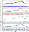 |
Fig. 2 DM time series and DM residuals recovered by EW (blue, first and second panels), DMX (red, third and fourth panels), and DM GP (green, fifth and sixth panels). The black line is the injected DM time series. In the last two panels, we overplot, respectively, the DM time series and the DM residuals for the three methods. The DM and RN injected parameters for this realization are: γRN = 3.7, γDM = 8/3, ARN = −12.6, and ADM = −13.3. |
4 Discussion
4.1 Absorption of red noise in the dispersion measure reconstruction
The presence of both RN and DM noise in our initial dataset allows us to compare the ability of each method to correctly identify the chromatic noise processes when achromatic signals are also present. The DM residuals reported in the top panel of Fig. 3 show that none of the methods that model RN display any evident structure. On the other hand, DM GP no RN and DMX no RN show evident corruptions in the DM recovery, whose structure matches the injected RN signal (bottom panel). The same conclusion can be drawn by looking at the first column of Figs. 4 and 5, in which the distributions of the normalized DM residuals calculated for those two methods are not symmetric and not centered around zero. This indicates that modeling by DM GP and DMX is not inherently restricted to modeling frequency-dependent signals, but is susceptible to absorbing frequency-independent signals as well, especially if those are not being independently modeled in the analysis. This is true as long as the RN signal is sufficiently “loud” to rise above the WN level. When this condition is not satisfied, or when the power spectrum of the RN exceeds the WN power by only a few frequency bins, then the DM recovery is not affected as much by the absence of RN modeling. This can easily be seen in the second and third columns of Figs. 4 and 5, where the distributions are very similar to each other because of the low amplitude of the RN (−13.3 and −14.3, respectively).
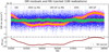 |
Fig. 3 Top panel: DM residuals of the 100 realizations for the five considered methods – EW(blue), DMX no RN (magenta), DM GP no RN (orange), DMX (red), and DM GP (green) – for the following set of input parameters: γRN = 3.7, γDM = 8/3, ARN = −12.6, and ADM = −13.3. Bottom panel: RN signal injected (the same for all of the 100 realizations; see Sect. 2). |
Mean uncertainty on the DM measurements for each method and pair of (ARN, ADM) in the case of γRN = 2.5, γDM = 3.2.
4.2 Comparison of the methods based on precision and accuracy
We have based our comparison of the methods on both the yielded precision and accuracy. We define precision as the uncertainty on the measured DM. The method that gives measurements with the lowest uncertainties, and that hence is the most precise, is DM GP, followed by DMX and then EW. This can be inferred from Tables 2 and 3, where we report the mean uncertainty on the DM recoveries for each method and set of parameters. The mean uncertainties of DM GP are around one order of magnitude smaller than the EW ones, while DMX sits in the middle of the two. When the noise model lacks the RN component (DMX no RN, DM GP no RN), and hence we fit the residuals only with the DM and WN, the mean DM uncertainty is systematically lower than for the full noise model that includes WN, RN, and DM. This is expected because without fitting for the RN we are reducing the number of parameters in the model. The behavior of the DM residuals when we consider all the 100 simulated realization together is shown in Fig. 3 for each of the five methods. The least precise method, EW, is also associated with the largest spread in the residuals, while DM GP (with RN modeled) produces a much smaller deviation of the residuals around zero.
While precision informs about the uncertainty level, it does not report how far the data points are from the true value. We define accuracy as the level of agreement between a test result and the true value3. The accuracy test was conducted by studying the histograms in Figs. 4 and 5. These were obtained by normalizing the DM residuals by their uncertainties, and hence offering a measure that serves as a proxy for the deviation of each bin in the histogram from the true value in terms of sigmas.
At first, we checked the fraction of residuals that lies within the 3σ threshold for each method, which for a Gaussian distribution is expected to be 99.7%. For EW, more than 99.9% of the values fall within 3σ, and this happens mostly because the uncertainties on the DM measurements are the highest among the methods. DMX is the second most accurate method, with a percentage of data points within 3σ greater than 99.5%, followed by DM GP with 98.5%. The remaining methods converge on higher percentages, comparable with the three just mentioned, only when the RN amplitude is at the lowest simulated level (−14.3).
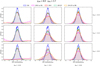 |
Fig. 4 Histograms of DM residuals normalized by their uncertainty for EW (blue), DMX no RN (magenta), DM GP no RN (orange), DMX (red), and DM GP (green). ARN decreases going from left to right (as is indicated at the bottom of the columns); ADM increases going upward (as is indicated on the right of each row). The spectral indices are γRN = 3.7 and γDM = 8/3. |
4.3 Whitening of the dispersion measure residuals
Other than precision and accuracy, we also investigated the ability of each method to whiten the DM residuals, meaning that we checked whether they are random and independent, without exhibiting correlated structures. This is extremely important for noise modeling, since any structure left in the DM residuals is associated with either the absorption of power in other noise components or with artifacts introduced by the method itself. We have conducted a Gaussianity test on the normalized DM residuals, and the associated reduced chi-squared values  are reported in Tables 4 and 5. For EW,
  , which implies that the data are well described by a Gaussian distribution and that there are no, or very few, remaining time-correlated structures in the DM residuals. For DMX,
  , showing that EW does not appreciably outperform DMX in whitening the DM residuals. For DMX no RN and DM GP no RN, the results are as expected: as long as ARN is high, they are not able to properly recover the DM values, and hence the
  associated with the histograms of the normalized residuals is very high. If ARN = −13.6, DMX no RN can reach
  values that are closer to 1 with respect to DM GP no RN, which does so only when ARN = −14.6. Lastly, DM GP, even though it is the most precise method, is not the most accurate and also not the best at whitening the DM residuals. The distributions in Figs. 4 and 5 are most of the time similar to the DMX ones, but the corresponding
  are not as close to 1. Time-correlated structures, both short- and long-term, are still present in DM GP DM residuals, emphasized by the aforementioned reduced error bars. The short-term time correlated structures are caused by the high- Fourier-frequency components of the injected signal (the highest of which is f30 = 30/Tspan), while long-term ones are mainly due to the presence of RN in the data. A more explicit representation of this feature is shown in Fig. 6, where the first two rows show DM residuals for a single realization and 100 realizations, respectively, using DM GP (similar results to DM GP can be obtained with DMX). The third row reports the comparison between the structure left in the DM residuals and the injected RN, showing that the DM modeling is indeed absorbing power from the RN process, as it displays the same signature as the injected RN signal. However, we also need to consider whether these structures have a significant impact on the timing residuals by comparing their power spectrum with the WN level. To do so, we computed a discrete Fourier transform and subsequently the power spectrum of the DM residuals at different ARN and compared it with the level of the WN injected for each of the three methods. The result is shown in Fig. 7. On average, the WN dominates over the DM residuals, which confirms that the signature remaining in the DM residuals cannot significantly be detected, and therefore will not affect the timing residuals. On the other hand, we can say that EW is not affected at all by the strength of the RN, while it significantly influences DM GP and DMX.
Importantly, Fig. 7 shows that the remaining power associated with the DM residuals is the lowest for DM GP (and DMX). This hints that DM GP (and DMX) diminishes the dispersive noise level in the ToAs to the minimum among the techniques tested, a result that would be beneficial in studies that need the most optimal noise mitigation possible. Hence, while a full study of the DM GP analysis and its interaction with various types of RN (particularly GWs) is beyond the scope of this paper, this finding indicates that DM GP (and DMX) might work best for whitening timing residuals; for example, in a context such as the search for low-frequency GWs.
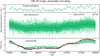 |
Fig. 6 The top panel shows the DM residuals obtained by applying DM GP (with RN modeling) to an individual simulation over the 100 realizations for values of the noise parameters ARN = −13.6, ADM = −13.3, γRN = 3.7, γDM = 8/3, EFAC and EQUAD as in Table 1, and σToA = 5 µs. The second panel reports an average of the DM residuals left by DM GP over the 100 simulations performed with the same parameters. The bottom panel shows the injected RN signal (red dots) compared to the time delay associated with the mean DM GP (shaded green). Note that we have a shaded region because a single DM value causes a frequency-dependent delay. Hence, the edges of the green region correspond to the maximum and minimum frequencies of the band. |
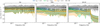 |
Fig. 7 Power spectra of the DM residuals left by the EW (left panel), DMX (central panel), and DM GP (right panel) methods. We also show the WN level (black) and the power spectra for different RN amplitudes: ARN = −14.6 (orange with vertical dashes); ARN = −13.6 (green with dots); and ARN = −12.6 (blue with oblique dashes). With DM GP, we modeled the noise up to a Fourier-frequency of 30/Tspan ~ 1.15 × 10⁻⁷ Hz, the same as the injected signal. That is why in the right-hand panel there is a drop at that specific frequency in the power spectrum of the DM GP residuals. |
4.4 Alternative simulation settings
Here, we test the methods on datasets that we simulated by varying specific settings. First, we reduced the uncertainties of the simulated ToAs from our initial value (from 5 to 1 µs and 0.1 µs) to improve our sensitivity to the RN process and DM variations, and then we simulated the ToAs at L-band frequencies. Finally, we changed the injected DM time series.
Mean DM uncertainty across methods (EW, DMX, DM GP) for simulated ToAs with fixed uncertainties of 1 and 0.1 µs.
4.4.1 Testing different time-of-arrival uncertainties
We used σtemp = 5 µs, since it represents the typical mean uncertainties on ToAs obtained from LOFAR observations (Donner et al. 2020). However, there might be pulsars with higher ToA precision, and we expect that future facilities such as the low- frequency part of the Square Kilometer Array (Janssen et al. 2015) will improve the ToA sensitivity. For this reason, we ran two new simulation sets, with decreased values for the σtemp, firstly at 1µs and then at 0.1 µs. Furthermore, as this reduces the WN floor level, we enhanced the methods’ capability to identify RN and properly disentangle it from DM variations. The WN parameters injected in the simulations were also changed to: EFAC = 1, EQUAD = 10−8 s. Chromatic and achromatic red processes were both set to 30 Fourier-frequency components, with γRN = 3.7, γDM = 8/3, ARN = −13.6, and ADM = −13.3.
In Table 6, we report the DM uncertainty levels for each method and each uncertainty. Given the smaller error bars of the ToAs, the precision on the DM measurements increases, as was expected. As we did previously, we can rank DM GP as the most precise method, followed by DMX and EW.
We recall that an important finding from our simulations (see Sect. 4.3) was about the RN signal left in the DM residuals. In fact, Fig. 6 (bottom panel) shows that the signal left in the DM residuals matches exactly the one of the injected RN. The corresponding delay, which is thus left on average in the timing residuals, is about ±2 µs. This changes in the two new cases characterized by low ToA uncertainties: when σtemp = 1 µs, the mean DM signal that is left due to an erroneous RN absorption contributes to the timing residuals at the level of ±150 ns; when σtemp = 0.1 µs, this becomes ±20 ns. Since the injected RN signal was the same, we can confirm that higher precision on the ToAs allows to increase the sensitivity to the RN and improve the accuracy of the measurements of DM variations.
4.4.2 Testing times of arrival in the L band
In this part, we report the results obtained by applying the DM computation methods to L-band ToAs. To simulate high- frequency ToAs, we refer to the data collected by the Nançay decimeter radiotelescope (NRT), which has a relatively large bandwidth (512 MHz) centered at 1.4 GHz divided into four subbands (EPTA Collaboration 2023). The input parameters were: EFAC = 1, EQUAD = 10−8 s, ADM = −13.3, and γDM = 8/3. We used a conservative 1 µs ToA template-fitting error.
Concerning the precision of the methods, the results are similar to the ones in the LOFAR frequency case: DM GP is the most precise, followed by DMX and EW. However, the size of these errors is now larger by approximately two orders of magnitude (see Table 7). This is due to two main reasons: the first is the increased central frequency of the analysed ToAs (which is 1.4 GHz against the 153 MHz of the previous LOFAR-like case), because DM is inversely proportional to the squared of the observing frequency. The second is the fractional bandwidth, B (see Eq. (5)): the higher B, the better the precision in the DM measurements (Verbiest & Shaifullah 2018). For the NRT-like case, B ≃ 0.34, while for the LOFAR-like case, B ≃ 0.41. Concerning accuracy, we also report similar conclusions as before: EW has more than 99.76% of the values within 3σ and it is the most accurate method, followed by DMX with more than 99.44% and finally DM GP with 99.2%. In addition, the Gaus- sianity test provides similar results to the LOFAR-like case. In Table 8 are listed the reduced χ2 values, which confirm that on average EW and DMX are marginally better at whitening the residuals due to their larger error bars (and thus lower precision), on single DM recoveries. In the top panel of Fig. 8 are presented the DM residuals for each of the three methods, while the corresponding normalized histograms are reported in the bottom plot. Figure 9 shows the power spectra of the DM residuals compared with the injected signal. Despite the fact that the WN is dominating in most of the frequency bins, all of the three methods can model the long-term structures present in the data. At the highest frequencies in the spectra, EW and DMX cannot match the injected signal anymore due to the limits imposed by the WN.
Instead, DM GP is the only method that produces a power spectrum that does not cross the injection line, meaning that it is not adding any more power at those frequencies. We note that DM GP uses a power-law model to describe the noise process, which is identical to the functional form of the injected signal. Therefore, it is possible that the reported results show a biased result for DM GP, since in real-life datasets we may not have pure power-law noise processes.
To evaluate a more realistic case, in the following section we test the methods on an injected DM time series that does not come from a pure power law.
Reduced χ2 of the normalized DM residuals.
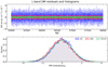 |
Fig. 8 Top panel: DM residuals left by the EW (blue), DMX (red), and DM GP (green) methods when run over the 100 realizations of L-band ToAs. Bottom panel: histograms of the DM residuals normalized by their uncertainty. The input noise parameters are ADM = −13.3 and γDM = 8/3. |
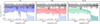 |
Fig. 9 Power spectra of the DM residuals obtained using EW (left), DMX (center), and DM GP (right), compared with the injected signal (light blue) in the L band. The input noise parameters are ADM = −13.3 and γDM = 8/3. The injected signal power (light-blue) drops at a frequency of 30/Tspan ~ 1.15 × 10⁻⁷ Hz. We used the same number of frequency components in the modeling with DM GP. |
 |
Fig. 10 DM time series injected in the data with an empirical power spectrum (Donner 2022). |
4.4.3 Custom dispersion measure injection
Here, we test the performance of the three considered techniques over an individual, injected DM time-series with an empirical power-spectrum shape, derived in Donner (2022) from the LOFAR dataset of PSR J0139+5814 (see Fig. 10). The ToAs are still evenly spaced, with an uncertainty set to 5µs, and the injected WN is defined by EFAC = 1.2 and EQUAD = 2 µs. Given the short timescale fluctuations in the injected signal, we used 107 Fourier components to define the power-spectrum used in DM GP, which corresponds to the limit imposed by the Nyquist theorem given the 215 data points. The result of the analysis are reported in Fig. 11, where we show the DM residuals in the top panel and their power spectra in the bottom panel. As was previously noted, EW and DMX provide independent DM measurements (although DMX might introduce some degree of correlations for close-by points; see Lam et al. 2017), while DM GP assumes an underlying model for the power spectrum to describe the DM variations. The DM GP error bars are now larger than the DMX ones, and hence the recoveries are extremely accurate. The bottom panel of Fig. 11 shows that even with the injected signal resembling a broken power law, DM GP is able to absorb the signal, and hence successfully recover the injected DM time series.
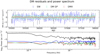 |
Fig. 11 DM residuals for EW (blue), DM GP (green), and DMX (red) obtained by taking the difference of the DMs recovered by each method and the injected DM time series of Fig. 10 with an unknown power spectrum. The WN parameters are EFAC = 1.2 and EQUAD 2 µs and the ToA uncertainty was set at 5 µs. Bottom panel: power spectra of the injected signal (black) and of the DM residuals. |
5 Conclusion
In this paper, we have carried out a series of simulations in order to test the performance of the three main methods available in the PTA community to calculate DM variations: EW, DM GP, and DMX. The final aim is to provide information on the calculation of the DM time series for, for example, studies of the IISM and the solar wind.
Our main conclusion is that, while they all perform well, the most accurate method of calculating DM variations is EW, but DM GP and DMX seem to lower the level of the DM noise in the timing residuals the most.
In more detail, we conclude that all of the methods perform satisfactorily (as long as the RN and DM models are selected correctly for DMX and DM GP). Figure 3 demonstrates that, when the RN power is significant, including it in the noise model is unavoidable; otherwise, the achromatic, time-correlated structures will be absorbed in the DM modeling in the cases of DMX and DM GP.
With respect to the precision, the mean uncertainties 〈σDM〉 on the DM recoveries for EW are independent of the amplitudes of the RN processes. This means that the method is only affected by the ToA precision and the frequency coverage of the data. For DMX and DM GP, instead, 〈σDM〉 depends on the amplitude of the injected RN process (see Tables 2 and 3). Overall, the method that gives the most precise DM measurements is DM GP.
We also studied the accuracy, defined as the level of agreement between a test result and the true value while taking into account the uncertainties, by analyzing the distributions of the normalized DM residuals (Figs. 4 and 5). Because of the larger error bars, EW is the most accurate method, having in most of the cases >99.9% of the data within 3σ. The second most accurate method, according to this criterion, is DMX, while DM GP is less accurate because of its high DM precision, which results in more data points in the tail of the distribution. This is true not only at LOFAR frequencies, but also in the L-band trials, where we simulated an NRT-like frequency coverage.
The accuracy test, though, as is described above, does not imply that the DM residuals are white. Hence, we have conducted a Gaussianity test on each of the normalized DM residuals distributions, which informs one about the ability of each method to remove time-correlated structures from the ToAs. The  of the Gaussian fits are reported in Tables 4 and 5, and they show that EW is the method with the narrowest range of
  around 1. DMX shows similar results, but only when the RN is modeled. However, the
  range shown by DMX fluctuates more than for EW. DM GP, which uses a linear combination of Fourier components, produces a time series where close data points are not completely independent. This affects the overall residual distribution, resulting in the widest
  range spanned among the three methods.
To better understand the reasons behind the DMX and DM GP distributions, we studied the effect of the RN on the DM residuals. In Fig. 6, we show that even when the RN is modeled, a signature can still be found in the DM residuals yielded by DM GP and DMX. This happens when the WN level exceeds the RN, especially at the highest Fourier frequencies. Nonetheless, Fig. 7 shows that, at LOFAR frequencies, the unmodeled RN signal remains below the WN level. In order to properly disentangle the RN and DM noise signal, it is necessary to have high-precision ToAs. In fact, we investigated this scenario by simulating datasets with reduced uncertainties, σToAs = 1 µs, 0.1 µs, and, as was expected, DMX and DM GP no longer show any significant structures related to the injected RN signal in the DM residuals. The aforementioned precision-accuracy hierarchy holds in this simulation scenario as well. Similar conclusions are reached in (albeit limited) simulations carried out in the L band and with an injected DM time series with an empirical spectral shape.
However, we stress that these results are based on simulations that do not take into account uneven observational cadence, variable ToA uncertainty, poor, if not absent, frequency coverage of the data, and also combination of datasets; in other words, the most common characteristics of real-life data. When these additional complexities are present, it is possible that DM GP performs better than other methods thanks to its flexibility and the fact that its characteristics allow a more optimal blending of data with diverse properties. Moreover, the performance of EW and DMX might be affected by more realistic datasets because of their windowing constraints. A firmer conclusion will be obtained once these scenarios are taken into consideration. Also, the impact of these DM recovery schemes on timing model parameters has not been assessed in our work, but Kramer et al. (2021) has already shown that astrometric parameters can be corrupted by some of the schemes tested. Consequently, future work on this topic would require a complete assessment of that aspect, as well.
Last, we reach the important conclusion that DM GP and DMX seem to have the capacity to reduce the DM noise level to the minimum (see Fig. 7). Future works should assess the effectiveness of the analyzed methods in modeling DM variations as a source of noise when a GW background is also present in the data.
Acknowledgements
F.I. is supported by the University of Cagliari (IT). F.I., C.T., A.P. are supported by the Istituto Nazionale di Astrofisica. A.C. and G.M.S. acknowledge financial support provided under the European Union’s H2020 ERC Consolidator Grant “Binary Massive Black Hole Astrophysics” (B Massive, Grant Agreement: 818691). J.P.W.V. acknowledges support from NSF AccelNet award No. 2114721. S.C.S. acknowledges the support of a College of Science and Engineering University of Galway Postgraduate Scholarship. M.T.L. graciously acknowledges support received from NSF AAG award number 2009468, and NSF Physics Frontiers Center award number 2020265, which supports the NANOGrav project. Work at NRL is supported by NASA.
Appendix A Evaluating time-domain realizations of stochastic time-correlated signals with LaForge
This part describes the method used in LAFORGE software to obtain time-domain realization of stochastic signals measured in the frequency domain. The stochastic and time-correlated signals in PTA data such as DM variations are mainly modeled as Gaussian processes (GPs). GPs are defined as a collection of (infinite) random variables representing the function values (e.g., time delay of the modeled signal in the timing residuals) for all input locations (i.e., observing epochs). Any finite set of these random variables has a joint Gaussian distribution. Thus, GPs allows us to define the mean value and the variance of the signal at any input location.
GPs can be fully specified with one of each following approaches (Rasmussen & Williams 2006):
-
Weight-space view, where the process is defined as a linear sum of deterministic basis functions Tµ(t) multiplied by weights aµ as
 (A.1)
(A.1)with µ = 1, …, m and where the weights are Gaussian random variables as
 , with
  assumed to be a zero vector in our case, and ϕµν corresponding to the weights covariance matrix.
The PTA likelihood including a GP described in the weightspace view can be written as
![Mathematical equation: $\eqalign{ & p\left( {\delta t\mid {a_\mu },GP} \right) = \cr & {{\exp \left[ { - {1 \over 2}\sum\nolimits_{i,j} {\left( {\delta {t_i} - \sum\nolimits_{\rm{\mu }} {{a_{\rm{\mu }}}} {T_{\rm{\mu }}}\left( {{t_i}} \right)} \right)} N_{ij}^{ - 1}\left( {\delta {t_j} - \sum\nolimits_{\rm{\mu }} {{a_{\rm{\mu }}}} {T_{\rm{\mu }}}\left( {{t_j}} \right)} \right)} \right]} \over {\sqrt {{{(2\pi )}^n}\det (N)} }} \cr & \times {{\exp \left[ { - {1 \over 2}\sum\nolimits_{{\rm{\mu ,}}v} {{a_{\rm{\mu }}}} \phi _{{\rm{\mu }}\nu }^{ - 1}{a_\nu }} \right]} \over {\sqrt {{{(2\pi )}^m}\det (\phi )} }}, \cr} $](/articles/aa/full_html/2024/12/aa50740-24/aa50740-24-eq30.png) (A.2)
(A.2)with δt and N respectively corresponding to the timing residuals and the covariance matrix, i, j = 1, …, n and µ, ν = 1, …, m.
-
Function-space view, where the GP directly describes the targeted signal as
 (A.3)
(A.3)including the mean function g(t) and the covariance function k(t, t′), also referred to as kernel.
The PTA likelihood in that form is marginalized over the basis weights mentioned above and can be expressed as
![Mathematical equation: $p(\delta t\mid {\rm{GP}}) = {{\exp \left[ { - {1 \over 2}\sum\nolimits_{i,j} \delta {t_i}{{\left( {{N_{ij}} + {K_{ij}}} \right)}^{ - 1}}\delta {t_j}} \right]} \over {\sqrt {{{(2\pi )}^n}\det (N + K)} }},$](/articles/aa/full_html/2024/12/aa50740-24/aa50740-24-eq32.png) (A.4)
(A.4)where K = k(t, t′).
In PTA analysis, we usually employ Eq. A.4 and express k(t, t′) from the correspondence between both views as (Rasmussen & Williams 2006)
 (A.5)
(A.5)
In practice, we set the basis functions T as a finite set of sine/cosine functions and
 (A.6)
(A.6)
with the right-hand side terms respectively corresponding to the power spectral density (PSD), the Kronecker delta and the time span of the data set. This approach corresponds to the Fourier- sum approach described in (van Haasteren & Vallisneri 2014).
To summarize, we use a time-domain likelihood function with a parameterized covariance matrix that contains a PSD that is most often defined as a simple power-law described with two parameters: the amplitude A, usually set at the reference frequency of 1 yr−1 and the spectral slope γ.
The Gaussian process signal in the time-domain f (t) can be evaluated from Eq. A.1 after estimating the weights a with Eq. A.2. Let us now describe a method to estimate realizations of a, where we perform a maximum likelihood estimation on Eq. A.2 (Lentati et al. 2013). Let us rewrite the logarithm of this equation in a matrix notation,
![Mathematical equation: $\matrix{ {\log [p(\delta t\mid a,GP)] = } & { - {1 \over 2}{{(\delta t - aT)}^{\rm{T}}}{N^{ - 1}}(\delta t - aT) - {1 \over 2}{a^{\rm{T}}}{\phi ^{ - 1}}a} \cr {} & { - {1 \over 2}[(n + m)\log (2\pi ) + \log (\det (N)\det (\phi ))],} \cr } $](/articles/aa/full_html/2024/12/aa50740-24/aa50740-24-eq35.png) (A.7)
(A.7)
where the third term is just a constant number “cst,” and thus
![Mathematical equation: $\matrix{ {\log [p(\delta t\mid a,GP)]} \hfill & { = - {1 \over 2}\left[ {\delta {t^{\rm{T}}}{N^{ - 1}}\delta t + {{(aT)}^{\rm{T}}}{N^{ - 1}}(aT) + {a^{\rm{T}}}{\phi ^{ - 1}}a} \right]} \hfill \cr {} \hfill & { + {{\left( {{T^{\rm{T}}}{N^{ - 1}}\delta t} \right)}^{\rm{T}}}a + {\rm{cst}}} \hfill \cr {} \hfill & { = - {1 \over 2}\left[ {\delta {t^{\rm{T}}}{N^{ - 1}}\delta t + {a^{\rm{T}}}\left( {{T^{\rm{T}}}{N^{ - 1}}T + {\phi ^{ - 1}}} \right)a} \right]} \hfill \cr {} \hfill & { + {{\left( {{T^{\rm{T}}}{N^{ - 1}}\delta t} \right)}^{\rm{T}}}a + {\rm{cst}}.} \hfill \cr } $](/articles/aa/full_html/2024/12/aa50740-24/aa50740-24-eq36.png) (A.8)
(A.8)
Let us now write its derivative over the weights,
![Mathematical equation: ${{\partial \log [p(\delta t\mid a,GP)]} \over {\partial a}} = \left( {{T^{\rm{T}}}{N^{ - 1}}T + {\phi ^{ - 1}}} \right)a - {\left( {{T^{\rm{T}}}{N^{ - 1}}\delta t} \right)^{\rm{T}}},$](/articles/aa/full_html/2024/12/aa50740-24/aa50740-24-eq37.png) (A.9)
(A.9)
and finally obtain the maximum likelihood vector of weights â,
 (A.10)
where we evaluate ϕ using Eq. A.6, for which P(f) is computed by using posterior distributions of our model parameters (e.g., A and γ if defined as a power-law) evaluated from a Bayesian analysis. Furthermore, N is computed after applying WN parameters (e.g., EFAC, EQUAD) with values taken from the same posterior distributions. This way, we evaluate time-domain realizations that are marginalized over other processes included during the Bayesian analysis.
Appendix B Achromatic noise recoveries with DMX and DM GP
In this section we report on how DMX and DM GP methods are able to recover achromatic noise parameters from our simulations.
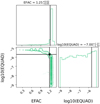 |
Fig. B.1 Corner plot of WN parameters using DM GP for an individual realization (see Sect. 2) with injected noise parameters: ADM = −13.3, γDM = −2.7, ARN = −13.6 and γRN = −3.7. Black lines correspond to the injected values. |
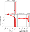 |
Fig. B.2 Corner plot of WN parameters using DMX for an individual realization (see Sect. 2) with injected noise parameters: ADM = −13.3, γDM = −2.7, ARN = −13.6 and γRN = −3.7. Black lines correspond to the injected values. |
B.1 White noise
WN parameters are inferred during the DMX and DM GP analysis through Eq. (6) in the enterprise software suite. Since in our simulations the ToA uncertainties are all the same, the EFAC and EQUAD parameters are strongly correlated as shown in Figs. B.1 and B.2. Overall, the EFAC parameters are always well constrained and consistent with the injected values for both DM GP and DMX. On the other hand, the EQUADs show a flat posterior (meaning that they are totally unconstrained) but still consistent with the injection. Moreover, DM GP tends to present a small peak at higher EQUADs, while DMX does not. In order to disentangle EFAC and EQUAD parameters, simulations with variable ToA uncertainties are required.
B.2 Achromatic red noise
In Figs. B.3 and B.4 we report the 100 posterior distributions of RN parameters obtained from the simulations described in Sect. 2. We show the only fiducial case with ADM = −13.3 and varying ARN. Enterprise can well constrain the RN parameters alongside DM GP and DMX as long as the power spectrum of the injected RN is above the WN floor (i.e., when ARN = −12.6 and barely for ARN = −13.6. See also Fig. 1). When this does not happen, the posterior distributions of ARN and γRN are flat and unconstrained. In all of the cases the recoveries are consistent with the injected values. This result is also confirmed when we reduce the ToA uncertainties to 1 or 0.1 µs, hence decreasing the WN power level. In these cases the RN parameters are well constrained and consistent with the injection even for lower ARN .
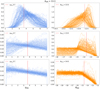 |
Fig. B.3 Posterior distributions of RN parameters using DM GP for 100 realizations (see Sect. 2) with injected DM noise parameters: ADM = −13.3, γDM = −2.7. On the left-hand column there is the spectral index γRN ; on the right-hand column there is the RN amplitude ARN . Each row correspond to a different injected ARN . Red vertical lines report the injected values. |
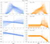 |
Fig. B.4 Posterior distributions of RN parameters using DMX for 100 realizations (see Sect. 2) with injected DM noise parameters: ADM = −13.3, γDM = −2.7. On th left-hand column there is the spectral index γRN ; on the right-hand column there is the RN amplitude ARN . Each row correspond to a different injected ARN . Red vertical lines report the injected values. |
References
- Agazie, G., Alam, M. F., Anumarlapudi, A., et al. 2023, ApJ, 951, L9 [CrossRef] [Google Scholar]
- Armstrong, J. W., Rickett, B. J., & Spangler, S. R. 1995, ApJ, 443, 209 [Google Scholar]
- Backer, D. C., Kulkarni, S. R., Heiles, C., Davis, M., & Goss, W. 1982, Nature, 300, 615 [NASA ADS] [CrossRef] [Google Scholar]
- Bondonneau, L., Grießmeier, J. M., Theureau, G., et al. 2021, A&A, 652, A34 [NASA ADS] [CrossRef] [EDP Sciences] [Google Scholar]
- Donner, J. Y. 2022, PhD thesis, Universität Bielefeld, Bielefeld, Germany [Google Scholar]
- Donner, J. Y., Verbiest, J. P. W., Tiburzi, C., et al. 2019, A&A, 624, A22 [NASA ADS] [CrossRef] [EDP Sciences] [Google Scholar]
- Donner, J. Y., Verbiest, J. P. W., Tiburzi, C., et al. 2020, A&A, 644, A153 [EDP Sciences] [Google Scholar]
- Edwards, R. T., Hobbs, G. B., & Manchester, R. N. 2006, MNRAS, 372, 1549 [Google Scholar]
- Ellis, J., & Van Haasteren, R. 2017, jellis18/PTMCMCSampler: Official Release [Google Scholar]
- Ellis, J. A., Vallisneri, M., Taylor, S. R., & Baker, P. T. 2020, Astrophysics Source Code Library [record ascl:1912.015] [Google Scholar]
- EPTA Collaboration (Antoniadis, J., et al.) 2023, A&A, 678, A48 [Google Scholar]
- EPTA Collaboration & InPTA Collaboration (Antoniadis, J., et al.) 2023, A&A, 678, A49 [Google Scholar]
- Foster, R. S., & Cordes, J. M. 1990, ApJ, 364, 123 [NASA ADS] [CrossRef] [Google Scholar]
- Hassall, T. E., Stappers, B. W., Hessels, J. W. T., et al. 2012, A&A, 543, A66 [NASA ADS] [CrossRef] [EDP Sciences] [Google Scholar]
- Hazboun, J. S. 2020, La Forge, https://zenodo.org/records/4152550 [Google Scholar]
- Hellings, R. W., & Downs, G. S. 1983, ApJ, 265, L39 [NASA ADS] [CrossRef] [Google Scholar]
- Hobbs, G., Lyne, A. G., Kramer, M., Martin, C. E., & Jordan, C. 2004, MNRAS, 353, 1311 [NASA ADS] [CrossRef] [Google Scholar]
- Hobbs, G., Lorimer, D. R., Lyne, A. G., & Kramer, M. 2005, MNRAS, 360, 974 [Google Scholar]
- Janssen, G., Hobbs, G., McLaughlin, M., et al. 2015, Proc. Sci., 14, 37 [Google Scholar]
- Jones, M. L., McLaughlin, M. A., Lam, M. T., et al. 2017, ApJ, 841, 125 [NASA ADS] [CrossRef] [Google Scholar]
- Keith, M. J., Johnston, S., Karastergiou, A., et al. 2024, MNRAS, 530, 1581 [NASA ADS] [CrossRef] [Google Scholar]
- Kramer, M., Stairs, I. H., Manchester, R. N., et al. 2021, Phys. Rev. X, 11, 041050 [NASA ADS] [Google Scholar]
- Krishnakumar, M. A., Manoharan, P. K., Joshi, B. C., et al. 2021, A&A, 651, A5 [Google Scholar]
- Lam, M. T., Cordes, J. M., Chatterjee, S., & Dolch, T. 2015, ApJ, 801, 130 [NASA ADS] [CrossRef] [Google Scholar]
- Lam, M. T., Cordes, J. M., Chatterjee, S., et al. 2016, ApJ, 821, 66 [NASA ADS] [CrossRef] [Google Scholar]
- Lam, M. T., Cordes, J. M., Chatterjee, S., et al. 2017, ApJ, 834, 35 [Google Scholar]
- Lentati, L., Alexander, P., Hobson, M. P., et al. 2013, Phys. Rev. D, 87, 104021 [NASA ADS] [CrossRef] [Google Scholar]
- Lorimer, D. R., & Kramer, M. 2005, Handbook of Pulsar Astronomy (Cambridge: Cambridge university press), 4 [Google Scholar]
- Luo, J., Ransom, S., Demorest, P., et al. 2021, ApJ, 911, 45 [NASA ADS] [CrossRef] [Google Scholar]
- Maggiore, M. 2018, Gravitational Waves: Astrophysics and Cosmology (Oxford: Oxford University Press), 2 [Google Scholar]
- Phinney, E. S. 2001, arXiv e-prints [arXiv:astro-ph/0108028] [Google Scholar]
- Rasmussen, C. E., & Williams, C. K. I. 2006, Gaussian Processes for Machine Learning (Cambridge, Massachusetts: The MIT Press) [Google Scholar]
- Rickett, B. J. 1990, ARA&A, 28, 561 [NASA ADS] [CrossRef] [Google Scholar]
- Taylor, S. R. 2021, arXiv e-prints [arXiv:2105.13270] [Google Scholar]
- Tiburzi, C. 2018, PASA, 35, e013 [Google Scholar]
- Tiburzi, C., Verbiest, J. P. W., Shaifullah, G. M., et al. 2019, MNRAS, 487, 394 [Google Scholar]
- Tiburzi, C., Shaifullah, G. M., Bassa, C. G., et al. 2021, A&A, 647, A84 [NASA ADS] [CrossRef] [EDP Sciences] [Google Scholar]
- Vallisneri, M. 2020, Astrophysics Source Code Library [record ascl:2002.017] [Google Scholar]
- van Haarlem, M. P., Wise, M. W., Gunst, A. W., et al. 2013, A&A, 556, A2 [NASA ADS] [CrossRef] [EDP Sciences] [Google Scholar]
- van Haasteren, R., & Vallisneri, M. 2014, Phys. Rev. D, 90, 104012 [NASA ADS] [CrossRef] [Google Scholar]
- Verbiest, J. P. W., & Shaifullah, G. M. 2018, Class. Quantum Gravity, 35, 133001 [NASA ADS] [CrossRef] [Google Scholar]
- Verbiest, J. P. W., Lentati, L., Hobbs, G., et al. 2016, MNRAS, 458, 1267 [Google Scholar]
- Verbiest, J. P. W., Osłowski, S., & Burke-Spolaor, S. 2021, Pulsar Timing Array Experiments (Singapore: Springer), 1 [Google Scholar]
- Zarka, P., Girard, J. N., Tagger, M., & Denis, L. 2012, in SF2A-2012: Proceedings of the Annual meeting of the French Society of Astronomy and Astrophysics, eds. S. Boissier, P. de Laverny, N. Nardetto, R. Samadi, D. Valls-Gabaud, & H. Wozniak, 687 [Google Scholar]
We have used the same convention as EPTA Collaboration & InPTA Collaboration (2023) for σToA; however, some PTA collaborations use the TEMPO2 definition (see Verbiest et al. 2016).
RN modeling is an inherent part of EW, so no separate analysis is possible.
ISO 5725-1:2023 in International Organization for Standardization (https://www.iso.org/home.html).
All Tables
Mean uncertainty on the DM measurements for each method and pair of (ARN, ADM) values in the case of γRN = 3.7, γDM = 8/3.
Mean uncertainty on the DM measurements for each method and pair of (ARN, ADM) in the case of γRN = 2.5, γDM = 3.2.
Mean DM uncertainty across methods (EW, DMX, DM GP) for simulated ToAs with fixed uncertainties of 1 and 0.1 µs.
All Figures
|
Fig. 1 Simulations carried out with injected values of γRN, ARN, and γDM of, respectively, 3.7, −13.3, and 8/3. The columns are associated with increasing values of ADM, left to right (as is indicated at the bottom). First row: 1 out of the 100 simulated timing residuals with a color map associated with the observing frequency (as is reported in the top right corner). Second row: injected RN signal. Third row: 1 out of the 100 different injections of the DM time series. On the right y axis, we report the corresponding time delay at the reference frequency of 150 MHz. Fourth row: Power spectra of the injected noise processes; WN (black), RN (red), and DM variations at LOFAR central frequency of the band of ~150 MHz (light blue). The dashed vertical gray lines are the 30 Fourier frequency bins. |
| In the text | |
|
Fig. 2 DM time series and DM residuals recovered by EW (blue, first and second panels), DMX (red, third and fourth panels), and DM GP (green, fifth and sixth panels). The black line is the injected DM time series. In the last two panels, we overplot, respectively, the DM time series and the DM residuals for the three methods. The DM and RN injected parameters for this realization are: γRN = 3.7, γDM = 8/3, ARN = −12.6, and ADM = −13.3. |
| In the text | |
|
Fig. 3 Top panel: DM residuals of the 100 realizations for the five considered methods – EW(blue), DMX no RN (magenta), DM GP no RN (orange), DMX (red), and DM GP (green) – for the following set of input parameters: γRN = 3.7, γDM = 8/3, ARN = −12.6, and ADM = −13.3. Bottom panel: RN signal injected (the same for all of the 100 realizations; see Sect. 2). |
| In the text | |
|
Fig. 4 Histograms of DM residuals normalized by their uncertainty for EW (blue), DMX no RN (magenta), DM GP no RN (orange), DMX (red), and DM GP (green). ARN decreases going from left to right (as is indicated at the bottom of the columns); ADM increases going upward (as is indicated on the right of each row). The spectral indices are γRN = 3.7 and γDM = 8/3. |
| In the text | |
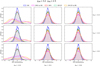 |
Fig. 5 As in Fig. 4, but the spectral indices are γRN = 2.5 and γDM = 3.2. |
| In the text | |
|
Fig. 6 The top panel shows the DM residuals obtained by applying DM GP (with RN modeling) to an individual simulation over the 100 realizations for values of the noise parameters ARN = −13.6, ADM = −13.3, γRN = 3.7, γDM = 8/3, EFAC and EQUAD as in Table 1, and σToA = 5 µs. The second panel reports an average of the DM residuals left by DM GP over the 100 simulations performed with the same parameters. The bottom panel shows the injected RN signal (red dots) compared to the time delay associated with the mean DM GP (shaded green). Note that we have a shaded region because a single DM value causes a frequency-dependent delay. Hence, the edges of the green region correspond to the maximum and minimum frequencies of the band. |
| In the text | |
|
Fig. 7 Power spectra of the DM residuals left by the EW (left panel), DMX (central panel), and DM GP (right panel) methods. We also show the WN level (black) and the power spectra for different RN amplitudes: ARN = −14.6 (orange with vertical dashes); ARN = −13.6 (green with dots); and ARN = −12.6 (blue with oblique dashes). With DM GP, we modeled the noise up to a Fourier-frequency of 30/Tspan ~ 1.15 × 10⁻⁷ Hz, the same as the injected signal. That is why in the right-hand panel there is a drop at that specific frequency in the power spectrum of the DM GP residuals. |
| In the text | |
|
Fig. 8 Top panel: DM residuals left by the EW (blue), DMX (red), and DM GP (green) methods when run over the 100 realizations of L-band ToAs. Bottom panel: histograms of the DM residuals normalized by their uncertainty. The input noise parameters are ADM = −13.3 and γDM = 8/3. |
| In the text | |
|
Fig. 9 Power spectra of the DM residuals obtained using EW (left), DMX (center), and DM GP (right), compared with the injected signal (light blue) in the L band. The input noise parameters are ADM = −13.3 and γDM = 8/3. The injected signal power (light-blue) drops at a frequency of 30/Tspan ~ 1.15 × 10⁻⁷ Hz. We used the same number of frequency components in the modeling with DM GP. |
| In the text | |
|
Fig. 10 DM time series injected in the data with an empirical power spectrum (Donner 2022). |
| In the text | |
|
Fig. 11 DM residuals for EW (blue), DM GP (green), and DMX (red) obtained by taking the difference of the DMs recovered by each method and the injected DM time series of Fig. 10 with an unknown power spectrum. The WN parameters are EFAC = 1.2 and EQUAD 2 µs and the ToA uncertainty was set at 5 µs. Bottom panel: power spectra of the injected signal (black) and of the DM residuals. |
| In the text | |
|
Fig. B.1 Corner plot of WN parameters using DM GP for an individual realization (see Sect. 2) with injected noise parameters: ADM = −13.3, γDM = −2.7, ARN = −13.6 and γRN = −3.7. Black lines correspond to the injected values. |
| In the text | |
|
Fig. B.2 Corner plot of WN parameters using DMX for an individual realization (see Sect. 2) with injected noise parameters: ADM = −13.3, γDM = −2.7, ARN = −13.6 and γRN = −3.7. Black lines correspond to the injected values. |
| In the text | |
|
Fig. B.3 Posterior distributions of RN parameters using DM GP for 100 realizations (see Sect. 2) with injected DM noise parameters: ADM = −13.3, γDM = −2.7. On the left-hand column there is the spectral index γRN ; on the right-hand column there is the RN amplitude ARN . Each row correspond to a different injected ARN . Red vertical lines report the injected values. |
| In the text | |
|
Fig. B.4 Posterior distributions of RN parameters using DMX for 100 realizations (see Sect. 2) with injected DM noise parameters: ADM = −13.3, γDM = −2.7. On th left-hand column there is the spectral index γRN ; on the right-hand column there is the RN amplitude ARN . Each row correspond to a different injected ARN . Red vertical lines report the injected values. |
| In the text | |
Current usage metrics show cumulative count of Article Views (full-text article views including HTML views, PDF and ePub downloads, according to the available data) and Abstracts Views on Vision4Press platform.
Data correspond to usage on the plateform after 2015. The current usage metrics is available 48-96 hours after online publication and is updated daily on week days.
Initial download of the metrics may take a while.