| Issue |
A&A
Volume 697, May 2025
|
|
|---|---|---|
| Article Number | A25 | |
| Number of page(s) | 13 | |
| Section | Astrophysical processes | |
| DOI | https://doi.org/10.1051/0004-6361/202348475 | |
| Published online | 01 May 2025 | |
The impact of outliers on pulsar timing array signals
1
Dipartimento di Fisica “G. Occhialini”, Università degli Studi di Milano-Bicocca, Piazza della Scienza 3, I-20126 Milano, Italy
2
INFN, Sezione di Milano-Bicocca, Piazza della Scienza 3, I-20126 Milano, Italy
3
INAF – Osservatorio Astronomico di Cagliari, Via della Scienza 5, 09047 Selargius (CA), Italy
4
INAF – Osservatorio Astronomico di Brera, Via Brera 20, I-20121 Milano, Italy
⋆ Corresponding author: This email address is being protected from spambots. You need JavaScript enabled to view it.
Received:
2
November
2023
Accepted:
16
March
2025
Abstract
The detection of gravitational waves with pulsar timing arrays (PTAs) requires precise measurements of the difference between the pulsars’ timing models and their observed pulses as well as dealing with numerous and sometimes hard-to-diagnose sources of noise. Outliers may have an impact on this already difficult procedure, especially if the methods used are not robust to such anomalous observations. Until now, no complete and practical quantification of their effects on PTA data has been provided. With this work, we aim to fill this gap. We corrupted simulated datasets featuring an increasing degree of complexity with varying percentages of uniformly distributed outliers and investigated the impact of the latter on the recovery of the injected gravitational wave signals and pulsar noise terms. We find that the gravitational wave signal, due to its expected correlation, is more robust against these anomalous observations when compared to the other injected processes. This result is especially relevant in the context of the emerging statistical evidence for the gravitational wave background in PTA datasets, further strengthening those claims.
Key words: gravitation / gravitational waves / methods: data analysis / pulsars: general
© The Authors 2025
 Open Access article, published by EDP Sciences, under the terms of the Creative Commons Attribution License (https://creativecommons.org/licenses/by/4.0), which permits unrestricted use, distribution, and reproduction in any medium, provided the original work is properly cited.
This article is published in open access under the Subscribe to Open model. This email address is being protected from spambots. You need JavaScript enabled to view it. to support open access publication.
1. Introduction
Supermassive (MBH > 108 M⊙) black hole binaries (SMBHBs) emit nanohertz frequency gravitational waves (GWs) during their slow and adiabatic inspiral phase (see, e.g., Sesana et al. 2008, and references therein). To observe them, it is necessary to exploit Galactic-scale detectors relying on sensitive long-term monitoring of astrophysical sources. The first, and currently most successful of these are PTAs (Foster & Backer 1990) operating in the radio frequencies, but similar detectors are being created by monitoring pulsars in the gamma rays (FERMI-LAT Collaboration 2022) or by monitoring several pairs of binary stars (Crosta et al. 2024). The PTAs consist of arrays of regularly monitored millisecond pulsars (Backer et al. 1982) whose extreme rotational stability, leading to their characteristic pulsed observations, is comparable with the precision of atomic clocks (see, e.g., Lorimer & Kramer 2004; Hobbs et al. 2020). Detection can be accomplished by comparing regularly recorded times-of-arrival (ToAs) of the pulses from each pulsar with theoretical predictions. The latter derives from a “pulsar timing” model of the pulsars describing their astrometry, rotational behavior, additional orbital effects if they are in binary systems, and the effects of any intervening sources of delays, such as the interstellar medium (ISM). The outcomes of this comparison are the pulsar timing residuals. As shown by Sazhin (1978), Detweiler (1979), Maggiore (2008), and others, when GWs cross the space between pulsars and the Earth, they perturb the local space-time along the propagation path of the pulses, inducing a correlated delay in the timing residuals of each pulsar. This correlation is a function of the angular separation between pulsar pairs, and follows the form predicted by Hellings & Downs (1983), henceforth, HD correlation. Recently, four major PTA collaborations, namely the European Timing Array and Indian Pulsar Timing Arrays (EPTA and InPTA, respectively; Ferdman et al. 2010; Joshi et al. 2022), the North American Nanohertz Observatory for Gravitational Waves (NANOGrav; Ransom et al. 2019), the Parkes Pulsar Timing Array (PPTA; Manchester et al. 2013), and the Chinese PTA (CPTA; Lee et al. 2016), presented evidence in their data for the presence of a correlated red noise process that follows the HD correlation. In addition, the team working on MeerTime (Bailes et al. 2020), the pulsar timing experiment at MeerKAT –the expanded Karoo Array Telescope in South Africa – have released their first PTA datasets (Spiewak et al. 2022). Together, all the “regional” PTAs, apart from the CPTA, are combining their datasets into a common global effort, the International PTA (IPTA; Verbiest et al. 2016; Perera et al. 2019), to increase the overall sensitivity of the datasets. The first gravitational signal that PTAs expect to observe is a stochastic GW background (GWB), most likely produced by the incoherent superposition of GWs generated by inspiralling SMBHBs (see, e.g., Rosado et al. 2015, and references therein). Due to the stochastic nature of this signal, it cannot be included in the deterministic pulsar timing model, and hence it shows up in the residuals. This effect is relatively weak, and working with an extremely precise timing model and high-quality data is necessary for successful detection. This task is even more challenging since the GWB is not the only contributor to the residuals. As shown in Chalumeau et al. (2021), there are also signatures of white (Gaussian or radiometer) noise and of pulsar intrinsic red noise (RN), or timing noise, which can mask the GWB. Finally, density fluctuations in the ionized ISM crossing the line of sight lead to another noise component, quantified as variations of the pulsar “dispersion measure” (DM). This can be particularly troublesome since it induces a similar delay in timing residuals as the GWB. However, the GWB can be distinguished from other noise sources through its characteristic HD correlation.
Apart from these competing noise sources, several systematics can pose challenges to extracting the contribution of the GWB from the timing residuals. One of these could be outliers, pathological observations that can emerge from a process different from those responsible for most of the data. The most common process for generating outliers in radio astronomical observations is radio frequency interference (RFI). A significant fraction of RFI is often easily identified and can be removed from observations. However, RFI rejection can be especially challenging when the interference is weak. Further, interference can also be generated as a result of the conversion from electromagnetic waves to electronic signals, or during the digitization step. Discussing the full range of possible contaminants in radio pulsar data is beyond the scope of this article (see Verbiest & Shaifullah 2018, for a more detailed summary). At the same time, pulsars are also known to display a variety of intrinsic changes in the pulse profile and propagation effects (see, e.g., Donner et al. 2019), which can also lead to large excursions away from the “timing model”. In the following analysis, we do not distinguish between systematic and astrophysical outliers.
Regardless of their specific origin, their presence cannot be ignored, especially when statistical techniques are applied to the data. The least-square fitting procedures (Rousseeuw & Leroy 2005) on which pulsar timing software such as TEMPO2 (Hobbs et al. 2006b) are based are particularly susceptible to the influence of outliers. As shown in Vallisneri & van Haasteren (2017) fix, the presence of such anomalous observations can bias the estimation of WN parameters. Some methods have been proposed to take care of outliers (Vallisneri & van Haasteren 2017; Wang et al. 2017) in the PTA framework, but given the different processing schemes adopted by different PTAs, these are yet to become part of standard analysis.
In this study, we examine the influence of outliers on the properties of the recovered common signals in PTA datasets. Specifically, we search for both, a common uncorrelated red noise (henceforth, CP) process as well as an HD correlated process, in realistic datasets with noise properties mirroring real data and including an increasing percentage of uniformly distributed outliers. We also search for such processes in datasets to which no common process is added. Using Bayesian model selection, we test for biased recovery when outliers are present in the data.
This investigation is critical, in light of the recent PTA discoveries. The significance of the reported HD-correlated signal ranges between 2σ and 4σ, thus not yet meeting the “golden standard" generally accepted to claim detection. Although consistent with an SMBHB origin, the measured spectral properties of this signal are in mild tension with vanilla models of circular-GW-driven SMBHB populations. The data favor a background with amplitude pushing towards the upper limit produced by astrophysical models (Izquierdo-Villalba et al. 2022) and are described by a power-law with a flatter spectral index than expected from a population of circularized SMBHBs. However, uncertainties in the measurements are large and caution should be taken when drawing strong astrophysical conclusions from them (see discussions in EPTA Collaboration & InPTA Collaboration 2024). It is therefore important to assess the robustness of detection and parameter estimation against potential biases arising from the presence of bad data.
The paper is organized as follows. We describe how we constructed the datasets and their characteristics in Section 2. We present the results of their analysis in Section 3. We interpret those results and discuss their implications for PTA real data analysis in Section 4 and summarize our main findings in Section 5.
2. Datasets and methods
2.1. Datasets for signal recovery analysis
We generated three PTA-like datasets with an increasing degree of realism employing libstempo (Vallisneri 2020), a Python interface to TEMPO2 (Hobbs et al. 2006a; Edwards et al. 2006). We simulate ToAs for 25 pulsars observed by the EPTA collaboration, whose data1 are available in the IPTA second data release (henceforth the IPTA DR2, Perera et al. 2019). We chose to retain the actual starting and ending dates of observations for each pulsar in the datasets, as well as the number of observations while varying the cadence to obtain a slightly more uniform yet irregular distribution of the observations.
The main difference between the three datasets is the number of observing frequencies and systems, and how we assigned the values of the WN parameters:
-
OneF dataset: We assume that for each pulsar, the observations have been performed at a single observing frequency with a single telescope;
-
TwoF dataset: We introduce two observing frequencies associated with a unique telescope;
-
MultiF dataset: We take, for each pulsar, the observing frequencies, observatories, and systems utilized in the actual IPTA DR2 dataset for those pulsars. For some of the analysis, we extend this dataset by 10 years, thus producing a MultiF+10yr dataset.
The increasing degree of complexity arises from the fact that early PTA analyses relied on band-integrated TOAs from narrow-band observations, typically from a small set of observing telescopes. In contrast, modern PTA datasets incorporate data from an increasing number of telescopes with very wide observing bands. Further, the ability to separate RN and DM processes is heavily dependent on the available frequencies. Finally, when combining data from many instruments, outliers can become difficult to identify. For instance, the bottom panel of Figure 1 is an excellent approximation of residual plots for data from the IPTA DR2.
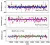 |
Fig. 1. Simulated timing residuals (colored circles) of PSR J1730−2304 with 10% of outliers injected (red crosses). The different colors of the timing residuals represent the systems responsible for the observations. The top plot represents the timing residuals simulated for the OneF dataset, for which we employ a single system/observation frequency for all the observations. In the central plot, we show those for the TwoF dataset for which we employ two systems/observation frequencies, and the bottom plot those for the MultiF dataset for which we consider several systems/observation frequencies. |
For the TwoF and MultiF datasets we also fitted constant offsets (JUMPs) to account for the use of multiple systems. To construct all the datasets, we first generated for each pulsar, idealized ToAs such that, when compared with the pulsar’s timing model, they return zero timing residuals. We assigned realistic uncertainties σToA to each observation and then, using our knowledge from real data analysis (see, e.g., Chalumeau et al. 2021), we injected white (or Gaussian) noise by rescaling them as follows:
 (1)
(1)
Here EFAC accounts for factorial imperfections in the white-noise quantification, whereas EQUAD accounts for potential additive sources of noise that are not naturally included in the formal ToA uncertainties σToA. The values of EFAC and EQUAD used change based on the dataset as reported in Table 1.
EFAC and EQUAD used in the simulated datasets. TNEF and TNEQ refer to the corresponding values reported in the parameters file of the pulsars considered.
For each pulsar, we injected timing noise, which consists of RN that can be modeled with a power-law power spectral density (PSD) function of the form
 (2)
(2)
where ARN is the RN amplitude and γRN is the spectral index. For this signal, we fix the number of Fourier modes to 30, following Chen et al. (2021). The values of the amplitude chosen for this work have been taken from the single pulsar noise analysis performed in Antoniadis et al. (2022).
In the MultiF dataset only, we also injected an achromatic DM noise, whose spectrum, specific for each pulsar, can be modeled exactly as the RN. We chose the amplitude and a spectral index, again following the analysis carried out in Antoniadis et al. (2022). Following Chen et al. (2021), we choose to use 100 Fourier modes to describe this signal. Finally, we add the GWB contribution to complete the datasets. As shown in Phinney (2001), the strain spectrum of GWB is expected to be well-modeled by a power-law:
 (3)
(3)
where AGWB and αGWB are the GWB strain amplitude and spectral index, respectively. The corresponding PSD 𝒫GWB can be parameterized as:
 (4)
(4)
with γGWB = 3 − 2αGWB. We set AGWB = 2 × 10⁻¹⁵, which is consistent with the current PTA estimates (Agazie et al. 2023b; EPTA Collaboration & InPTA Collaboration 2023; Reardon et al. 2023; Xu et al. 2023) and we consider γGW = 13/3, which is expected for a GWB generated by a population of SMBHBs on circular orbits whose evolution is driven by GW emission (Phinney 2001). For this signal, we fix the number of Fourier modes to 5 as done in Arzoumanian et al. (2020), Agazie et al. (2023b). After generating the datasets, we corrupted them by injecting outlier observations. Simulated timing residuals follow a Gaussian distribution with zero mean and variance σ. We define as outliers a small amount of randomly chosen data that follows the same distribution but with a very different variance, σout. As shown in Wang & Taylor (2021), an outlier indicator zi can be used to describe a corrupted dataset:
 (5)
(5)
In this way, it is possible to express the i-th timing residuals ri of a pulsar as:
 (6)
(6)
where we indicate with =ri, in the generated and non-corrupted i-th timing residuals. Following this definition, we assign zi = 1 to a certain percentage of randomly selected ToAs per pulsar, and we choose the value of σi, out such that the outliers have no relation with the majority of the data. Here σi, out is defined as σi, out = α σi where α is a positive or negative random number with absolute value ∈[3, 5] and σi is the post-fit timing residual root-mean-square (RMS). The percentages of outliers tested were 0% (i.e., uncorrupted data), 0.3%, 1%, 5% and 10%. In Figure 1 we show, as an example, the timing residuals (colored circles) of PSR J1730−2304 for the three datasets simulated and with 10% outliers injected (red crosses).
2.2. Datasets for model selection
To conduct the model selection analysis, we employed simulated datasets that were produced like that of the datasets given in Section 2.1, but without injecting the GWB. Similarly, three separate datasets have been produced (OneF, TwoF, MultiF) and subsequently tainted with outliers.
2.3. Statistical inference
To gauge the impact of outliers on the recovery of the signal injected, we first examine the simulated outliers-corrupted datasets and we estimate the parameters describing the noises of interest (RN, DM and GWB) using a PTA-specific Bayesian inference method (van Haasteren & Levin 2012; Ellis & van Haasteren 2017; Ellis et al. 2020) as employed in Perera et al. (2019), Arzoumanian et al. (2020), Chen et al. (2021), Goncharov et al. (2021), Agazie et al. (2023a), EPTA Collaboration & InPTA Collaboration (2023) and others. Then, we search for, along with the other signals, an additional common uncorrelated process (CP), which we modeled as a power-law with an amplitude ACP and a spectral index γCP, considering 30 Fourier modes. This noise behaves exactly as the pulsar RN, but with the main difference that the amplitude and the spectral index are the same for each pulsar (in the same fashion as the gravitational signal), but without including any spatial correlation. In this way, we test whether the presence of outliers can also introduce a spurious common process.
Bayesian inference is based on the Bayes theorem, which states that in order to obtain the posterior probability distributions of the parameters of interest, the likelihood, and the parameters’ prior probability distributions have to be specified. In terms of the latter, we kept the WN parameters (EFAC and EQUAD) fixed to the injected values (see Table 1), and we used uniform priors for the RN, DM-induced noise, GWB, and CP spectral indices (γ ∈ [0, 7]) and log-uniform priors for their amplitudes (log ARN, DM, CP ∈ [ − 20, −10], log AGWB ∈ [ − 18, −13]). The choice of these distributions closely follows Arzoumanian et al. (2020) and Chen et al. (2021).
The likelihood can be constructed by assuming that the timing residuals rai of the array’s a-th pulsar, measured at the i-th time, are made up of a deterministic  and a stochastic component. The former includes, for example, the effects due to the pulsar spin-down, the annual variations due to the poor knowledge of the pulsar positions in the sky, the uncertainties in the location of the Solar System barycenter (SSB), and the phase offsets or JUMPs due to changes in the equipment, that is, all the effects that can be modeled and included in the timing model. The latter includes the contributions from the intrinsic RN and WN processes, the DM-induced noise, the clock noise, any common and uncorrelated noise process and the GWB signal. Therefore, it is possible to write
 (7)
(7)
where  is the contribution related to an eventual uncorrelated CP,
  is the stochastic GWB contribution, and raiN is due to all other stochastic noise sources. Regarding the latter, we considered only the contributions of the RN, DM-induced noise, and WN. Similarly to Maggiore (2008), van Haasteren et al. (2009), van Haasteren & Levin (2012), we assumed that both the CP, the GWB and the noise components N are stochastic Gaussian processes, and thus they are fully characterized by their two-point correlation functions that can be represented by the covariance matrices:
 (8)
(8)
The timing residuals are then distributed as a multidimensional Gaussian and the likelihood is defined as:
 (9)
(9)
where θ includes all the parameters characterizing the timing model, the RN, the DM-induced noise, the WN, the CP, and the GWB; C(ai) (bj) is the total covariance matrix defined as:
 (10)
(10)
where δab is the Kronecker delta, βab = 1 for any value of a and b (pulsar indices) due to the uncorrelated but common nature of the CP, αab = 1 for a = b, while when a ≠ b, αab coincide with the HD function multiplied by 3/2:
 (11)
(11)
where θab is the relative angle between two pulsars. It is important to notice that the intrinsic RN and CP differentiate from the GWB since the latter induces an inter-pulsar correlation between timing residuals. Therefore, because of GWs, the timing residuals of each pulsar are both time (within the pulsar) and spatially correlated (across the array). A scheme of the structure of this matrix is shown in Figure 2.
 |
Fig. 2. Schematic representation of the covariance matrix for five pulsars (PSR). On the diagonal (auto-correlation), the contribution of the WN, RN, DM, CP, and GWB signals are present, while in the off-diagonal parts (cross-correlations), there is just that of the GWB. |
We used the Enhanced Numerical Toolbox Enabling a Robust PulsaR Inference SuitE (enterprise; Ellis et al. 2020) to define the prior probability distributions and construct the likelihood, and then we used the Parallel Tempering Markov chain Monte Carlo (PTMCMC; Ellis & van Haasteren 2017) sampling with 106 iterations to evaluate the posterior probabilities for the parameters of interest.
2.4. Model selection analysis
This analysis closely follows the methods and the models used in Zic et al. (2022) and Arzoumanian et al. (2020). We used the software enterprise_extensions (Taylor et al. 2021) to build the models and perform the comparison. In this case, we only inject WN, RN, DM-induced noise, and outliers (see Sec. 2.2). We then analyze the data with the three different models reported in Table 2. Also in this case we modeled the CP, present in CP1 and CP2, as a power law described by an amplitude ACP, a spectral index γCP and 30 Fourier components. For CP1 we use a log-uniform prior on the amplitude (log ACP ∈ [ − 20, −10]) and a uniform prior on the spectral index (γCP ∈ [0, 7]). In the case of CP2, we employed the same prior as in CP1 for the amplitude but we fixed the spectral index to 13/3. The model TN (which stands for timing noise) does not include a common process. Having defined the models, we used the product-space approach (Arzoumanian et al. 2020) to pick the one that better describes the data, between CP1 and TN and between CP2 and TN. This method involves creating a new variable: the model index, which is then sampled along with the parameters of the competing models. By evaluating the proportion of samples in each bin of the model index parameter, we were then able to evaluate the posterior odds ratio, following the hyper-model method (see, e.g., Hee et al. 2016).
Models compared in this analysis analysis.
3. Results
3.1. GWB and pulsar noise recovery in presence of outliers
The results obtained from the runs which consider a model with WN (fixed), RN, DM-induced noise (for MultiF dataset only) and GWB are summarized in Table 3. The effect of outliers on the GWB parameter recovery for the three datasets are reported in Figures 3, 4 and 5. We found the parameters describing the GWB to be, at worst, only weakly affected by the presence of outliers in any percentage studied. It has been possible to recover values of AGWB and γGWB consistently with those injected, within the 95% credible interval. The recovery occurs correctly and independently from the degree of realism of the dataset. Thus, these results show that the amount of outliers injected in these datasets is not enough to consistently affect the recovery of the parameters describing the GWB signal. Although some effects can be observed, they are limited principally to a slight broadening of the posterior distributions or to a small shift away from the expected center and they are observed only when 5% and 10% outliers are injected. The results of the analysis of the data with 10% injected outliers are not shown in Figure 5. With such a large fraction of outliers, the examination of the MultiF chains revealed sampling issues, making it difficult to produce reliable results. We believe the other percentages studied to be adequate to analyze the impact of outliers in the MultiF dataset since it is highly improbable that such a percentage (10%) of outliers could be present in real PTA datasets.
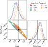 |
Fig. 3. Two-dimensional marginalized posterior distributions of log10AGWB and γGWB recovered for the OneF dataset corrupted with 0% (red), 0.3% (blue), 1% (green), 5% (pink) and 10% (orange) of outliers. Each pair of distributions (log10AGW; γGW) has been recovered separately and then overlapped to be easily compared. The black lines and the square indicate the injected values of the amplitude and spectral index. |
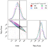 |
Fig. 5. Same as Figure 3 but for the MultiF dataset. In this case, the results for 10% of outliers injected are missing. Probably due to the high complexity of such dataset we were not able to obtain robust results for this case. However, it is very improbable to have data containing such a high percentage of outliers and the other percentages analyzed can be considered sufficient to study the influence of outliers in this dataset. |
Recovery performance of the uncorrelated CP and the GWB.
In contrast to the GWB, the recovery of the parameters describing the pulsars RNs and DM-induced noises is strongly affected by outliers. Regarding the RNs, already with 1% of outliers, the recovered posteriors of the amplitudes and of the spectral indices systematically shift with respect to those recovered from the uncorrupted datasets. In particular, those of the amplitudes tend to move toward the upper limit of the prior range employed in the analysis, while those of the spectral indices tend to move toward the lower limit. For both these parameters, the posteriors tend to become narrower as the number of outliers increases. In Figures 6, 7, and 8, we present cumulative marginalized posterior distributions for the amplitudes and spectral indices of the RNs across the three datasets under consideration. These distributions illustrate the cumulative effect of varying percentages of outliers. Specifically, each histogram, corresponding to a certain outlier percentage, represents the sum of all normalized marginalized posteriors of the amplitude or spectral index of the pulsars’ RNs. As can be observed, as the percentage of outliers increases the cumulative distributions of log10A and γ move, respectively, toward higher and lower values, becoming narrower and narrower. This implies that, in the presence of outliers, the intrinsic RN of pulsars is recovered almost as a higher-amplitude-WN since the spectral indices generally tend to cluster around 0 and the amplitudes tend to increase by almost 2 orders of magnitude.
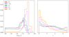 |
Fig. 6. Cumulative marginalized posterior distributions of the amplitudes (left) and the spectral indices (right) of pulsars’ RNs for the dataset OneF corrupted with 0% (red), 0.3% (blue), 1% (green), 5% (pink), and 10% (orange) of outliers. The histograms, in both panels, are the sum of the normalized marginalized posteriors of the amplitudes and the spectral indices of the RN of each pulsar. |
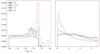 |
Fig. 8. Same as Figure 6 but for the dataset MultiF. As done in Figure 5, the distributions for the data corrupted with 10% of outliers are not reported. |
We observe a similar trend, albeit less pronounced, for the recovered DM-induced noise in the MultiF dataset, as depicted in Figure 9, where we show the distributions for the amplitudes and spectral indices of such noise. In the case of uncorrupted data, the amplitudes and spectral indices are weakly constrained, and the shift towards higher amplitudes and smaller spectral indices, due to outliers, is less prominent. This can be attributed to the challenging nature of recovering this signal, primarily due to its frequency-dependent characteristics. Successful constraining would require multiple observations at various frequencies for each epoch. The MultiF dataset is designed to emulate real EPTA data, where achieving an optimally diverse frequency coverage is often unfeasible. This inherent lack of sensitivity across the entire observed period constrains our ability to accurately recover the DM models.
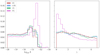 |
Fig. 9. The cumulative marginalized posterior distributions of the amplitudes (left) and the spectral indices (right) of the DM-induced noise specific for each pulsar for the dataset MultiF corrupted with 0% (red), 0.3% (blue), 1% (green), 5% (pink) of outliers. The histograms, in each panel, are the sum of the normalized marginalized posteriors of the amplitudes and the spectral indices of the DM-induced noises of the pulsars. As done in Figures 5, 8, the distributions for the data corrupted with 10% of outliers are not reported. |
3.2. Spurious common process due to outliers
Once we established the effects of outliers on the recovery of an injected GWB and intrinsic pulsar noises, we checked whether the presence of outliers can lead to the spurious detection of an uncorrelated CP. To this aim, we considered the same data used in Sec. 3.1 (which include a GWB and outliers) but we added an uncorrelated CP, modeled as a power law (ACP; γCP), to the recovery model. We also added, for each dataset (OneF, TwoF, MultiF), a test run in which we consider data with no outliers and no GWB injected and perform a search for RN, DM, and CP by fixing the WN parameters. This was done to check whether a CP could emerge in datasets that are not corrupted by outliers and in which no correlated common signal (e.g., a GWB) is present. The uncorrelated CPs and the GWB recoveries are reported, for each dataset, in Figures 10, 11 and 12. For the OneF dataset, the GWB can be recovered within the 95% credible interval consistently with the results reported for this dataset in Section 3.1. Alongside the GWB, it is possible to recover, independently from the number of outliers, a well-constrained CP which evolution depends on the severity of the contamination – as the number of outliers increase, the CP recovered moves toward higher amplitudes and lower spectral indices. This kind of evolution is the same that has been observed for the RNs and DMs as reported in Section 3.1. In contrast to the other datasets, the test search conducted on the TwoF dataset revealed the presence of a CP. This suggests that sources other than the outliers and the GWB might be capable of inducing a CP in this dataset. However, after injecting the GWB, this particular feature is less evident. A CP is again distinctly detected when at least 1% of outliers are injected into the data. Once recovered, this signal follows the same evolution as observed for the OneF dataset. In the case of the MultiF dataset, while the measured uncorrelated CP follows the same trends seen in the other datasets, a markedly different behavior can be observed for the GWB signal. When conducting a joint search for the GWB and a CP within this dataset, we observed that well-constrained posterior probabilities for the parameters characterizing the GWB cannot be obtained, whereas the opposite holds for the CP. This phenomenon is particularly prominent when fewer than 5% outliers are introduced into the dataset. Interestingly, with a 5% outlier presence in the data, it becomes feasible to effectively constrain the GWB. The latter result may be attributed to the fact that, when a relatively high percentage of outliers is introduced, the CP signal induced becomes distinctly discernible from the GWB signal, allowing the latter to emerge more clearly. On the other hand, the inability to recover the GWB in the presence of other outlier percentages can be attributed to the degree of realism of this dataset and the resemblance between the gravitational signal and the CP. The GWB signal, as described in Section 1, is formed by an uncorrelated part (auto-correlation terms along the diagonal of the matrix in Figure 2) and by a correlated part (cross-correlation terms in the off-diagonal part of the matrix in Figure 2) which is expected to be weaker with respect to the former, due to the magnitude of the correlation coefficients (αab ≤ 0.5 for a ≠ b). Therefore, it has been hypothesized that the auto-correlated component of the GWB signal should be the first to be observed (Romano et al. 2021; Pol et al. 2021). This was confirmed by real data, where a common red signal was first detected, and then evidence for correlation started to emerge. Pol et al. (2021) demonstrate that effective evidence for the cross-correlation component could be observed when, the datasets that they had examined, had a time span of ∼18 − 20 years. When an uncorrelated CP is searched alongside the GWB in our most realistic dataset, MultiF, it is possible that part of the auto-correlation component of the GWB flows into the power of the uncorrelated CP and the cross-correlated part is unable to emerge with sufficient strength to be constrained, resulting in the recovery shown in the left plot of Figure 12. Following similar reasoning as Romano et al. (2021) and Pol et al. (2021), we introduced the dataset MultiF+10Y, which extends the original MultiF dataset by an additional 10 years. We retained the same number of observations, uncertainties, frequencies, systems, and observatories. In confirmation of our hypothesis, with this dataset it is possible to recover the GWB within the 95% credible interval.
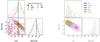 |
Fig. 10. Recovered common processes searched in the OneF dataset corrupted with 0% (red), 0.3% (blue), 1% (green), 5% (pink) and 10% (orange) of outliers. Left: two-dimensional posterior probabilities of the parameters characterizing the GWB (AGWB,γGWB). The injected values (2 × 10⁻¹⁵, 4.3) are represented by black lines and a square symbol. Notably, in this case, the signal can consistently be accurately recovered. Right: two-dimensional posterior probabilities of the parameters characterizing the CP (ACP,γCP). Unlike the GWB, this signal was not directly injected into the data. |
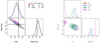 |
Fig. 12. Same as Figure 10 but for the MultiF dataset. In this scenario, when searching for the GWB in conjunction with an uncorrelated CP, successful recovery is not achievable when the data contains less than 5% outliers. However, with the presence of 5% outliers, successful recovery becomes possible. |
3.3. Model selection
To further study outliers as possible sources of spurious uncorrelated CP able to contribute to the signal detected in real PTA data analysis, we conducted a model comparison analysis applying the method presented in Sec. 2.4, considering the models reported in Table 2 and employing the datasets presented in Section 2.2.
3.3.1. CP1 versus TN
For each dataset considered, we observed increasing evidence in support of CP1 over TN, with the growth being correlated with the percentage of outliers injected. According to Table 4, in which we have reported the log10 posterior odds ratios resulting from the model comparison, when 0 to 1% of outliers are injected, there is weak but gradually growing support for CP1, while when 5% and 10% of outliers are present in the data, this support becomes fairly substantial. In Figure 14 are reported the uncorrelated CPs detected in this analysis, together with the that measured, considering the same model for the CP, in Chen et al. (2021). Where the evidence in support of CP1 over TN is weak, the posterior distributions for log10ACP and γCP are semi or unconstrained, as can be noticed from the error bars representing the 68% credible interval. As soon as the data contains from 5% to 10% of outliers, the presence of an uncorrelated CP becomes clear. The evolution of the amplitude and the spectral index with the number of outliers resembles those of the RNs of the pulsars or of the uncorrelated CP recovered in Secs. 3.1 and 3.2. Notably, the uncorrelated CP that can be recovered when 1% (5%) of outliers is present in the TwoF (MultiF) dataset, tends to overlaps with the CP recovered in the EPTA DR2 (Chen et al. 2021).
Posterior odds ratios for models CP1 and TN expressed in log10 scale.
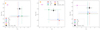 |
Fig. 14. Uncorrelated CP recovered from the comparison between the models CP1 and TN for the datasets OneF (left), TwoF (center), and MultiF (right) dataset corrupted with 0% (red), 0.3% (blue), 1% (green), 5% (pink), and 10% (orange) of outliers. The error bars represent the 68% credible interval. The uncorrelated CP recovered, modeling the CP as done in CP1, in Chen et al. (2021) is represented in black. |
3.3.2. CP2 versus TN
We also observed increasing evidence in support of CP2 over TN, with the growth being correlated with the percentage of outliers injected for the OneF and TwoF datasets. According to Table 5, when in the data are present from 0 to 1% of outliers, there is weak and slowly growing support for CP2, and with 5% and 10% of outliers, this support becomes fairly substantial, in particular for the dataset TwoF. The MultiF dataset behaves slightly differently showing no evidence either in support of or against the CP2 model over TN. It can be noticed that the posterior odds ratios given in Table 5 are orders of magnitude smaller than those reported in Table 4, especially those associated with the largest percentages of outliers, indicating that the CP2’s support against TN is weaker than the CP1’s. This agrees with the findings of Sec. 3.2. The uncorrelated CP found there was characterized by a relatively shallow slope, comparable to that found in the comparison between the CP1 and TN models. Therefore, we expect models that fix the spectral index at 13/3 to be less supported. The amplitudes of the CP recovered for these datasets are reported and compared with that found in Chen et al. (2021), while searching for the same kind of signal, in Figure 15. For the OneF dataset where the evidence in support of CP2 over TN is weak, ACP is unconstrained. When the percentage of outliers grows, so does the support for CP2, and the posteriors become constrained and well-defined. Conversely, even with no or a few outliers, the recovered CP amplitude is always tightly constrained for the TwoF dataset. The fact that a well-constrained amplitude can be recovered even in the absence of outliers in the data suggests, as already observed in Section 3.2, that some other property (other than outliers or GWB) of the data may be culprit, making it difficult to definitively pinpoint outliers as the primary cause of CP in this dataset. However, outliers have a significant impact on the CP when examining the strong change in amplitude as the number of outliers increases. Finally, despite the large number of outliers in the MultiF dataset, the recovered amplitude of the CP is never constrained. We note that, in general, the amplitudes retrieved do not change as dramatically as those of the CPs recovered from the comparison between CP1 and TN. The majority of the values we recovered tend to overlap with those identified in Chen et al. (2021). Notably, our findings are especially relevant when considering the TwoF dataset. When we introduce a 10% outlier contamination into the dataset, the amplitude we recover closely matches that observed in real data. However, it is essential to emphasize that this type of analysis does not provide sufficient evidence to claim the detection of a GWB. Nevertheless, it is reasonable to conclude that outliers have the potential to introduce a CP component comparable to what is observed in real data and could have contributed to it.
Posterior odds ratios for models CP2 and TN expressed in log10 scale.
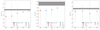 |
Fig. 15. Amplitudes of the CP found from the comparison between the models CP2 and TN for the datasets OneF (left), TwoF (center) and MultiF (right) dataset corrupted with 0% (red), 0.3% (blue), 1% (green), 5% (pink) and 10% (orange) of outliers. The error bars represent the 68% credible interval. The black band represent the value of the amplitude recovered, modeling the CP as in CP2, in Chen et al. (2021). |
4. Discussion
4.1. The influence of outliers on signal recovery
Based on the results presented in Section 3, we found that for a GWB signal in the loud regime (AGW ≳ 2 × 10⁻¹⁵) injected in an outliers-corrupted dataset, the recovered signal is always well-constrained and close to the injected value. However, even the smallest percentage of outliers caused a failure of RN and DM-induced noise parameters recovery. These three processes, which behave very similarly in the individual pulsar datasets since they all induce a time (auto-)correlation between timing residuals, have one significant difference: the GWB also induces a correlation between the timing residuals of different pulsars. Due to this propriety of the GWB, its recovery is largely unaffected by the presence of even a significant number of outliers (10% of the data, in the worst case scenario we considered).
4.2. The nature of the PTA covariance matrix and its implications on the signal recovery robustness
The likelihood in Eq. (9) depends on the product of timing residuals and on the inverse of their covariance matrix (van Haasteren et al. 2009). Specifically, the products of timing residuals are divided by the corresponding elements of the theoretically calculated covariance matrix and then summed together. This process is iterated over different parameter values. Better timing parameter estimates decrease this sum, maximizing the likelihood, while incorrect values decrease it. Given the particular shape of the covariance matrix, we now show that the most affected parameters are those lying on the diagonal part of the matrix.
Consider an N × N block matrix (see Figure 2 for an example) where  , and a identifies a specific pulsar. Here, Np represents the number of pulsars in the array, and n denotes the number of timing residuals per pulsar. Assume that there are y na outliers for each pulsar, where y is a percentage value ranging from 0 to 1. The number of permutations of n distinct objects grouped k at a time can be written as:
 (12)
(12)
To evaluate the number of encounters of an outlier with the other timing residuals, we set k = 2, reducing Eq. (12) to n(n − 1). Given a diagonal na × na block matrix with y na outliers, the number of intersections is then y na(y na − 1). Comparing this number to the total number of possible encounters (na2) gives us the encounter density along the diagonal of the covariance matrix of an array of Np pulsars:
 (13)
(13)
The WN, RN, DM-induced noise, and the auto-correlated part of the GWB all contribute to this part of the matrix, as shown in Figure 2. The density of encounters in the off-diagonal parts of the covariance matrix, which corresponds to the cross-correlated part of the GWB, is
 (14)
(14)
If y na ≫ 1, as we would expect for realistic PTA datasets such as IPTA DR2, the following approximations can be made:  and ρoff ∼ y2, which leads to:
 (15)
(15)
Thus the most sensitive part of the covariance matrix is the diagonal, where the encounter density is the highest. The RN and DM-induced noise parameters, lying exclusively on that diagonal, are the most strongly affected compared to the off-diagonal dominated GWB parameters. Notably, the density ratio of Eq. (15) scales inversely with the number of pulsars, showing that the GWB recovery is made more robust by adding more pulsars.
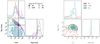 |
Fig. 13. Same as Figure 10 but for the MultiF+10Y dataset. This dataset is identical to the MultiF dataset, except a time span extended by 10 years. This extension significantly enhances sensitivity to the GWB, leading to a more pronounced emergence of the correlated component of the signal (left). However, it was not feasible to accurately generate posterior probability distributions for the CP when 5% of outliers were present; hence, these results have not been included (right). |
4.3. Outliers as sources of an uncorrelated CP
Having determined the influence of outliers on the recovery of the signals injected, we investigate outliers as a possible source of common uncorrelated RN, as this can still contribute to the signal recently observed by the major PTA collaborations. We added to the model used in Section 3.1 an uncorrelated CP modeled as a power-law characterized by an amplitude ACP and a spectral index γCP and then we searched for all the other parameters (RN, DM, GWB) along with it. After testing our datasets to check if no uncorrelated CP could be detected before the injection of the GWB or outliers, we discovered that for the majority of the dataset, injecting the GWB without outliers wassufficient to detect an uncorrelated CP. This feature, as underlined in Section 3.2, could be related to some power coming from the auto-correlation part of the GWB signal, which is detected as an uncorrelated CP. After adding outliers, the presence of a CP process became clear in each dataset studied.
In agreement with the findings in Section 3.1, outliers do not influence the GWB recovery but affect that of the uncorrelated CP. In general, an evolution of ACP toward larger values (∼10−13) and of γCP toward the lower limit of the prior space (∼0) is readily seen, in each dataset, as the number of outliers increases highlighting a correlation between such signal and outliers. However, it is crucial to stress that, except for the MultiF dataset, proper recovery of the GWB can always be achieved when the latter is searched along with an uncorrelated CP. If a model without an additional CP is utilized, the GWB can still be retrieved from the MultiF dataset despite outliers (see Section 3.1), and the failure of the recovery during this analysis is only due to a “split” of power between the uncorrelated CP and the GWB.
To have a clear picture of the uncorrelated CP originating from outliers, we performed the model comparisons presented in Section 3.3. From those, it is clear that an uncorrelated CP can be measured if a high enough percentage of outliers is present (≥1%) in the data, and its proprieties are strictly related to their abundance.
Figures 6, 7, 8 and 9 show why we can detect a CP when outliers contaminate data. Zic et al. (2022) demonstrated that if the RNs of the pulsars share very similar amplitudes and spectral indices, it is possible to detect an uncorrelated CP from data that do not contain it. In particular this CP is characterized by an amplitude and spectral index that resemble those of the pulsars. As explained in Section 4.1, the RNs and DMs are the processes that are most affected by outliers, which cause their amplitudes and spectral indices to cluster, respectively, toward the upper and lower limits of their prior spaces. As a result, outliers are responsible for causing the pulsars to share very similar properties in terms of the RN and DM, thus leading to the recovery of a spurious CP. Since the severity of the distortion in the RN/DM depends on the number of outliers, the characteristics of the CP recovered vary with it.
5. Conclusion
In light of the recent evidence for the GWB presented by PTAs (EPTA Collaboration & InPTA Collaboration 2023; Agazie et al. 2023b; Reardon et al. 2023; Xu et al. 2023), we presented the first attempt to quantify how much those results can be affected by the presence of bad data (i.e., outliers) in PTA data streams. To this end, we tried to answer the following three questions: a) How can outliers influence the detection of the signals characterizing PTA data? b) Could outliers be the source of a CP? c) Could outlier-induced CP mimic the early appearance of a GWB? As a starting point to answer these questions, we used three PTA datasets with an increasing degree of similarity to IPTA DR2, including characteristic sources of noise such as RN, WN (then kept fixed during the analysis), DM-induced noise, and a GWB. We then corrupted these datasets with specific types and percentages of outliers. To respond to the first query, we considered a model that parameterized the same injected signals and we evaluated its performance in the presence of outliers. The results of this analysis, reported in Section 3.1, showed that the RN and DM-induced noise parameters were strongly affected by the smallest percentage of outliers, while the estimate of the GWB is robust against any percentage injected, and this behavior can be deduced from the particular shape of the likelihood used to perform parameter estimation.
To answer the second question, we added to the recovery model an uncorrelated CP modeled as a power-law characterized by ACP and γCP. For all the datasets, an uncorrelated CP, whose characteristics change with the number of outliers injected, is recovered. This indicates that outliers can be a source of a spurious CP. For some datasets, we also find that, as soon as the GWB is injected into the data without outliers, an uncorrelated CP is recovered alongside the GWB. In the most extreme case, which has been observed when considering the MultiF dataset, only an uncorrelated CP could be recovered, burying the GWB (see Figure 12). The HD curve predicts that the correlated component of the GWB is weaker than the uncorrelated one; therefore, some of the power of the GWB may have leaked into the uncorrelated CP, making it more challenging to identify the GWB as a correlated process. This behavior was indeed predicted by Romano et al. (2021), Pol et al. (2021). They proposed that the GWB will likely first appear as an uncorrelated CP before becoming a spatially correlated signal as data gain enough sensitivity with time. We increased the time period of the MultiF dataset by 10 years and found that this is indeed the case (see Figure 13).
To answer the third question, we performed a model comparison following Zic et al. (2022), considering data in which no GWB had been injected but there were the contributions of WN, RN, DM-induced noise and outliers. We examined models that included an uncorrelated CP with a power-law shape and a variable or fixed spectral index versus models that do not. We found strong support for the models that include a CP, confirming once more that outliers can be sources of such a signal and can potentially contribute to the uncorrelated component of the signal recently observed.
These answers enabled us to draw the following important conclusions. When a GWB is present in the data, no outliers can successfully obscure or obliterate the signal (if the data are sensible enough to recover it). Therefore, the pipelines currently used to analyze PTA data are robust against outliers when it comes to characterizing a GWB. However, outliers can significantly impair the detection of RN and DM-induced noise, potentially leading to an uncorrelated CP. We found that such a signal, whose properties depend on the nature and quantity of outliers, can in some cases be compatible with, or at least contribute to, the uncorrelated RN component recently observed. Finally, we underline once more that while the results obtained can be used as an indication of the behavior of PTA data streams in the presence of outliers, they depend on the specific quality of outliers (both in quantity and type) considered, as well as on the noises injected and the methods used to simulate the dataset.
Available at https://gitlab.com/IPTA/DR2
Acknowledgments
We are deeply grateful to Aurélien Chalumeau and Joris Verbiest for several helpful discussions. The authors acknowledge the support of colleagues in the EPTA. GF is supported by the European Union’s H2020 ERC Starting Grant No. 945155–GWmining and Cariplo Foundation Grant No. 2021-0555. AS and GS acknowledge the financial support provided under the European Union‘s H2020 ERC Consolidator Grant “Binary Massive Black Hole Astrophysics” (B Massive, Grant Agreement: 818691).
References
- Agazie, G., Alam, M. F., Anumarlapudi, A., et al. 2023a, ApJ, 951, L9 [CrossRef] [Google Scholar]
- Agazie, G., Anumarlapudi, A., Archibald, A. M., et al. 2023b, ApJ, 951, L8 [NASA ADS] [CrossRef] [Google Scholar]
- Antoniadis, J., Arzoumanian, Z., Babak, S., et al. 2022, MNRAS, 510, 4873 [NASA ADS] [CrossRef] [Google Scholar]
- Arzoumanian, Z., Baker, P. T., Blumer, H., et al. 2020, ApJ, 905, L34 [NASA ADS] [CrossRef] [Google Scholar]
- Backer, D. C., Kulkarni, S. R., Heiles, C., Davis, M. M., & Goss, W. M. 1982, Nature, 300, 615 [NASA ADS] [CrossRef] [Google Scholar]
- Bailes, M., Jameson, A., Abbate, F., et al. 2020, Publ. Astron. Soc. Aust., 37, e028 [Google Scholar]
- Chalumeau, A., Babak, S., Petiteau, A., et al. 2021, MNRAS, 509, 5538 [NASA ADS] [CrossRef] [Google Scholar]
- Chen, S., Caballero, R. N., Guo, Y. J., et al. 2021, MNRAS, 508, 4970 [NASA ADS] [CrossRef] [Google Scholar]
- Crosta, M., Lattanzi, M. G., Le Poncin-Lafitte, C., et al. 2024, Sci. Rep., 14, 5074 [Google Scholar]
- Detweiler, S. 1979, ApJ, 234, 1100 [NASA ADS] [CrossRef] [Google Scholar]
- Donner, J. Y., Verbiest, J. P. W., Tiburzi, C., et al. 2019, ApJ, 624, A22 [Google Scholar]
- Edwards, R. T., Hobbs, G. B., & Manchester, R. N. 2006, MNRAS, 372, 1549 [Google Scholar]
- Ellis, J., & van Haasteren, R. 2017, https://doi.org/10.5281/zenodo.1037579 [Google Scholar]
- Ellis, J. A., Vallisneri, M., Taylor, S. R., & Baker, P. T. 2020, Astrophysics Source Code Library [record ascl:1912.015] [Google Scholar]
- EPTA Collaboration& InPTA Collaboration (Antoniadis, J., et al.) 2023, A&A, 678, A50 [CrossRef] [EDP Sciences] [Google Scholar]
- EPTA Collaboration& InPTA Collaboration (Antoniadis, J., et al.) 2024, A&A, 690, A118 [NASA ADS] [CrossRef] [EDP Sciences] [Google Scholar]
- Ferdman, R. D., van Haasteren, R., Bassa, C. G., et al. 2010, Class. Quantum Grav., 27, 084014 [Google Scholar]
- FERMI-LAT Collaboration (Ajello, M., et al.) 2022, Science, 376, 521 [NASA ADS] [CrossRef] [Google Scholar]
- Foster, R. S., & Backer, D. C. 1990, ApJ, 361, 300 [NASA ADS] [CrossRef] [Google Scholar]
- Goncharov, B., Shannon, R. M., Reardon, D. J., et al. 2021, ApJ, 917, L19 [NASA ADS] [CrossRef] [Google Scholar]
- Hee, S., Handley, W. J., Hobson, M. P., & Lasenby, A. N. 2016, MNRAS, 455, 2461 [NASA ADS] [CrossRef] [Google Scholar]
- Hellings, R. W., & Downs, G. S. 1983, ApJ, 265, L39 [NASA ADS] [CrossRef] [Google Scholar]
- Hobbs, G., Edwards, R., & Manchester, R. 2006a, ChJAA, 6, 189 [Google Scholar]
- Hobbs, G. B., Edwards, R. T., & Manchester, R. N. 2006b, MNRAS, 369, 655 [Google Scholar]
- Hobbs, G., Guo, L., Caballero, R. N., et al. 2020, MNRAS, 491, 5951 [Google Scholar]
- Izquierdo-Villalba, D., Sesana, A., Bonoli, S., & Colpi, M. 2022, MNRAS, 509, 3488 [Google Scholar]
- Joshi, B. C., Gopakumar, A., Pandian, A., et al. 2022, Journal of Astrophysics and Astronomy, 43, 98 [Google Scholar]
- Lee, K. J. 2016, in Frontiers in Radio Astronomy and FAST Early Sciences Symposium 2015, eds. L. Qain, & D. Li, ASP Conf. Ser., 502, 19 [Google Scholar]
- Lorimer, D. R., & Kramer, M. 2004, Handbook of Pulsar Astronomy, (Cambridge: Cambridge University Press), 4 [Google Scholar]
- Maggiore, M. 2008, Gravitational Waves (Oxford: Oxford University Press), 2 [Google Scholar]
- Manchester, R. N., Hobbs, G., Bailes, M., et al. 2013, Publ. Astron. Soc. Aust., 30, e017 [Google Scholar]
- Perera, B. B. P., DeCesar, M. E., Demorest, P. B., et al. 2019, MNRAS, 490, 4666 [Google Scholar]
- Phinney, E. S. 2001, MNRAS, submitted [arXiv:astro-ph/0108028] [Google Scholar]
- Pol, N. S., Taylor, S. R., Kelley, L. Z., et al. 2021, ApJ, 911, L34 [NASA ADS] [CrossRef] [Google Scholar]
- Ransom, S., Brazier, A., Chatterjee, S., et al. 2019, BAAS, 51, 195 [Google Scholar]
- Reardon, D. J., Zic, A., Shannon, R. M., et al. 2023, ApJ, 951, L6 [NASA ADS] [CrossRef] [Google Scholar]
- Romano, J. D., Hazboun, J. S., Siemens, X., & Archibald, A. M. 2021, Phys. Rev. D, 103, 063027 [Google Scholar]
- Rosado, P. A., Sesana, A., & Gair, J. 2015, MNRAS, 451, 2417 [NASA ADS] [CrossRef] [Google Scholar]
- Rousseeuw, P., & Leroy, A. 2005, Robust Regression and Outlier Detection, Wiley Series in Probability and Statistics (Wiley) [Google Scholar]
- Sazhin, M. V. 1978, Astron. Zh., 55, 65 [Google Scholar]
- Sesana, A., Vecchio, A., & Colacino, C. N. 2008, MNRAS, 390, 192 [NASA ADS] [CrossRef] [Google Scholar]
- Spiewak, R., Bailes, M., Miles, M. T., et al. 2022, The MeerTime Pulsar Timing Array - A Census of Emission Properties and Timing Potential (Cambridge: Cambridge University Press) [Google Scholar]
- Taylor, S. R., Baker, P. T., Hazboun, J. S., Simon, J., & Vigeland, S. J. 2021, enterprise-extensions, v2.3.3, https://github.com/nanograv/enterprise_extensions [Google Scholar]
- Vallisneri, M. 2020, Astrophysics Source Code Library [record ascl:2002.017] [Google Scholar]
- Vallisneri, M., & van Haasteren, R. 2017, MNRAS, 466, 4954 [Google Scholar]
- van Haasteren, R., & Levin, Y. 2012, MNRAS, 428, 1147 [Google Scholar]
- van Haasteren, R., Levin, Y., McDonald, P., & Lu, T. 2009, MNRAS, 395, 1005 [NASA ADS] [CrossRef] [Google Scholar]
- Verbiest, J. P. W., & Shaifullah, G. M. 2018, Class. Quantum Grav., 35, 133001 [Google Scholar]
- Verbiest, J. P. W., Lentati, L., Hobbs, G., et al. 2016, MNRAS, 458, 1267 [Google Scholar]
- Wang, Q., & Taylor, S. R. 2021, Bulletin of the American Astronomical Society, 53, 335.15 [Google Scholar]
- Wang, Y., Keith, M. J., Stappers, B., & Zheng, W. 2017, MNRAS, 468, 2637 [Google Scholar]
- Xu, H., Chen, S., Guo, Y., et al. 2023, Res. Astron. Astrophys., 23, 075024P [Google Scholar]
- Zic, A., Hobbs, G., Shannon, R. M., et al. 2022, MNRAS, 516, 410 [NASA ADS] [CrossRef] [Google Scholar]
All Tables
EFAC and EQUAD used in the simulated datasets. TNEF and TNEQ refer to the corresponding values reported in the parameters file of the pulsars considered.
All Figures
|
Fig. 1. Simulated timing residuals (colored circles) of PSR J1730−2304 with 10% of outliers injected (red crosses). The different colors of the timing residuals represent the systems responsible for the observations. The top plot represents the timing residuals simulated for the OneF dataset, for which we employ a single system/observation frequency for all the observations. In the central plot, we show those for the TwoF dataset for which we employ two systems/observation frequencies, and the bottom plot those for the MultiF dataset for which we consider several systems/observation frequencies. |
| In the text | |
|
Fig. 2. Schematic representation of the covariance matrix for five pulsars (PSR). On the diagonal (auto-correlation), the contribution of the WN, RN, DM, CP, and GWB signals are present, while in the off-diagonal parts (cross-correlations), there is just that of the GWB. |
| In the text | |
|
Fig. 3. Two-dimensional marginalized posterior distributions of log10AGWB and γGWB recovered for the OneF dataset corrupted with 0% (red), 0.3% (blue), 1% (green), 5% (pink) and 10% (orange) of outliers. Each pair of distributions (log10AGW; γGW) has been recovered separately and then overlapped to be easily compared. The black lines and the square indicate the injected values of the amplitude and spectral index. |
| In the text | |
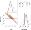 |
Fig. 4. Same as Figure 3 but for the TwoF dataset. |
| In the text | |
|
Fig. 5. Same as Figure 3 but for the MultiF dataset. In this case, the results for 10% of outliers injected are missing. Probably due to the high complexity of such dataset we were not able to obtain robust results for this case. However, it is very improbable to have data containing such a high percentage of outliers and the other percentages analyzed can be considered sufficient to study the influence of outliers in this dataset. |
| In the text | |
|
Fig. 6. Cumulative marginalized posterior distributions of the amplitudes (left) and the spectral indices (right) of pulsars’ RNs for the dataset OneF corrupted with 0% (red), 0.3% (blue), 1% (green), 5% (pink), and 10% (orange) of outliers. The histograms, in both panels, are the sum of the normalized marginalized posteriors of the amplitudes and the spectral indices of the RN of each pulsar. |
| In the text | |
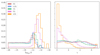 |
Fig. 7. Same as Figure 6 but for the dataset TwoF. |
| In the text | |
|
Fig. 8. Same as Figure 6 but for the dataset MultiF. As done in Figure 5, the distributions for the data corrupted with 10% of outliers are not reported. |
| In the text | |
|
Fig. 9. The cumulative marginalized posterior distributions of the amplitudes (left) and the spectral indices (right) of the DM-induced noise specific for each pulsar for the dataset MultiF corrupted with 0% (red), 0.3% (blue), 1% (green), 5% (pink) of outliers. The histograms, in each panel, are the sum of the normalized marginalized posteriors of the amplitudes and the spectral indices of the DM-induced noises of the pulsars. As done in Figures 5, 8, the distributions for the data corrupted with 10% of outliers are not reported. |
| In the text | |
|
Fig. 10. Recovered common processes searched in the OneF dataset corrupted with 0% (red), 0.3% (blue), 1% (green), 5% (pink) and 10% (orange) of outliers. Left: two-dimensional posterior probabilities of the parameters characterizing the GWB (AGWB,γGWB). The injected values (2 × 10⁻¹⁵, 4.3) are represented by black lines and a square symbol. Notably, in this case, the signal can consistently be accurately recovered. Right: two-dimensional posterior probabilities of the parameters characterizing the CP (ACP,γCP). Unlike the GWB, this signal was not directly injected into the data. |
| In the text | |
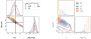 |
Fig. 11. Same as Figure 10 but for the TwoF dataset. |
| In the text | |
|
Fig. 12. Same as Figure 10 but for the MultiF dataset. In this scenario, when searching for the GWB in conjunction with an uncorrelated CP, successful recovery is not achievable when the data contains less than 5% outliers. However, with the presence of 5% outliers, successful recovery becomes possible. |
| In the text | |
|
Fig. 14. Uncorrelated CP recovered from the comparison between the models CP1 and TN for the datasets OneF (left), TwoF (center), and MultiF (right) dataset corrupted with 0% (red), 0.3% (blue), 1% (green), 5% (pink), and 10% (orange) of outliers. The error bars represent the 68% credible interval. The uncorrelated CP recovered, modeling the CP as done in CP1, in Chen et al. (2021) is represented in black. |
| In the text | |
|
Fig. 15. Amplitudes of the CP found from the comparison between the models CP2 and TN for the datasets OneF (left), TwoF (center) and MultiF (right) dataset corrupted with 0% (red), 0.3% (blue), 1% (green), 5% (pink) and 10% (orange) of outliers. The error bars represent the 68% credible interval. The black band represent the value of the amplitude recovered, modeling the CP as in CP2, in Chen et al. (2021). |
| In the text | |
|
Fig. 13. Same as Figure 10 but for the MultiF+10Y dataset. This dataset is identical to the MultiF dataset, except a time span extended by 10 years. This extension significantly enhances sensitivity to the GWB, leading to a more pronounced emergence of the correlated component of the signal (left). However, it was not feasible to accurately generate posterior probability distributions for the CP when 5% of outliers were present; hence, these results have not been included (right). |
| In the text | |
Current usage metrics show cumulative count of Article Views (full-text article views including HTML views, PDF and ePub downloads, according to the available data) and Abstracts Views on Vision4Press platform.
Data correspond to usage on the plateform after 2015. The current usage metrics is available 48-96 hours after online publication and is updated daily on week days.
Initial download of the metrics may take a while.