| Issue |
A&A
Volume 687, July 2024
|
|
|---|---|---|
| Article Number | A253 | |
| Number of page(s) | 19 | |
| Section | Cosmology (including clusters of galaxies) | |
| DOI | https://doi.org/10.1051/0004-6361/202449460 | |
| Published online | 17 July 2024 | |
Simulating the LOcal Web (SLOW)
II. Properties of local galaxy clusters
1
Universitäts-Sternwarte, Fakultät für Physik, Ludwig-Maximilians-Universität München, Scheinerstr.1, 81679 München, Germany
e-mail: hernandez@usm.lmu.de
2
Max Planck Institute for Astrophysics, Karl-Schwarzschild-Str. 1, 85741 Garching, Germany
3
Univ. Lille, CNRS, Centrale Lille, UMR 9189 CRIStAL, 59000 Lille, France
4
Université Paris-Saclay, CNRS, Institut d’Astrophysique Spatiale, 91405 Orsay, France
5
Leibniz-Institut für Astrophysik (AIP), An der Sternwarte 16, 14482 Potsdam, Germany
6
Astronomy Unit, Department of Physics, University of Trieste, Via Tiepolo 11, 34131 Trieste, Italy
7
ICSC – Italian Research Center on High Performance Computing, Big Data and Quantum Computing, Italy
8
INAF – Osservatorio Astronomico di Trieste, Via Tiepolo 11, 34131 Trieste, Italy
9
P.N. Lebedev Physical Institute of the Russian Academy of Sciences, Profsojuznaja 84/32, Moscow 117997, Russia
Received:
2
February
2024
Accepted:
9
April
2024
Context. This is the second paper in a series presenting the results from a 500 h−1Mpc large constrained simulation of the local Universe (SLOW). The initial conditions for this cosmological hydro-dynamical simulation are based on peculiar velocities derived from the CosmicFlows-2 catalog. The simulation follows cooling, star formation, and the evolution of super-massive black holes. This allows one to directly predict observable properties of the intracluster medium (ICM) within galaxy clusters, including X-ray luminosity, temperatures, and the Compton-y signal.
Aims. Comparing the properties of observed galaxy clusters within the local Universe with the properties of their simulated counterparts enables us to assess the effectiveness of the initial condition constraints in accurately replicating the mildly nonlinear properties of the largest, collapsed objects within the simulation.
Methods. Based on the combination of several, publicly available surveys we compiled a sample of galaxy clusters within the local Universe, of which we were able to cross-identify 46 of them with an associated counterpart within the SLOW simulation. We then derived the probability of the cross identification based on mass, X-ray luminosity, temperature, and Compton-y by comparing it to a random selection.
Results. Our set of 46 cross-identified local Universe clusters contains the 13 most massive clusters from the Planck SZ catalog as well as 70% of clusters with M500 larger than 2 × 10¹⁴ M⊙. Compared to previous constrained simulations of the local volume, we found in SLOW a much larger amount of replicated galaxy clusters, where their simulation-based mass prediction falls within the uncertainties of the observational mass estimates. Comparing the median observed and simulated masses of our cross-identified sample allows us to independently deduce a hydrostatic mass bias of (1 − b)≈0.87.
Conclusions. The SLOW constrained simulation of the local Universe faithfully reproduces numerous fundamental characteristics of a sizable number of galaxy clusters within our local neighborhood, opening a new avenue for studying the formation and evolution of a large set of individual galaxy clusters as well as testing our understanding of physical processes governing the ICM.
Key words: methods: numerical / galaxies: clusters: general / large-scale structure of Universe
© The Authors 2024
 Open Access article, published by EDP Sciences, under the terms of the Creative Commons Attribution License (https://creativecommons.org/licenses/by/4.0), which permits unrestricted use, distribution, and reproduction in any medium, provided the original work is properly cited.
This article is published in open access under the Subscribe to Open model. Subscribe to A&A to support open access publication.
1. Introduction
Extremely interesting times for cosmology and astrophysics are ahead of us. Within the past years, tremendous efforts have been put into developing missions to achieve larger cosmological surveys, for example the Sloan Digital Sky Survey (SDSS; Kollmeier et al. 2019), the Dark Energy Survey (DES; Dark Energy Survey Collaboration et al. 2016), and the 2df Galaxy Redshift Survey (2dFGRS; Colless et al. 2001), as well as deeper local surveys, for example the Arecibo Legacy Fast ALFA Survey (ALFALFA; Saintonge 2007), the Two Micron All Sky Survey (2MASS; Skrutskie et al. 2006), and the Nearby Galaxies Legacy Survey (NGLS; Wilson et al. 2009).
The progress in this field has been accompanied by the constant development of higher resolution hydrodynamical cosmological simulations (e.g., Balogh et al. 2004; Vogelsberger et al. 2014; Hirschmann et al. 2014; Dolag et al. 2016; Dubois et al. 2016), which have become a fundamental theoretical tool in the study of the multi-scale and nonlinear nature of astrophysical and cosmological processes (Overzier 2016).
Among the structures under study in our Universe, galaxy clusters represent a fundamental set of cosmological probes. Lying at the intersection between astrophysics and cosmology, the understanding of the formation and evolution of these structures is primordial in our comprehension of the Universe, spanning from the scale of particle physics, such as in the study of dark matter candidates (e.g., Treumann et al. 2000; Kaplan et al. 2009; Meissner & Nicolai 2019), to the largest cosmological scales when, for example, aiming to tight the constraints on cosmological parameters (e.g., Mantz et al. 2010b, 2015; de Haan et al. 2016; Schellenberger & Reiprich 2017; Pacaud et al. 2018; Ider Chitham et al. 2020; Chiu et al. 2023).
Nevertheless, retrieving detailed information about galaxy clusters through observations is indirect and may suffer from biases. Thus, the use of cosmological simulations has turned out to be a unique complementary tool in the study of the formation of these structures and to assess possible biases in the observations (see e.g., Kravtsov & Borgani 2012; Frenk & White 2012; Vogelsberger et al. 2020, for more extensive reviews).
Traditionally, what we call standard cosmological simulations of structure formation, such as Magneticum (Hirschmann et al. 2014; Dolag et al. 2016), Horizon-AGN (Dubois et al. 2016), EAGLE (Schaye et al. 2015), and IllustrisTNG (Pillepich et al. 2018), have aimed to produce “random” statistically representative patches of the Universe. Even if these simulations can reflect properties of our Universe in a statistical manner, such as large-scale structure, clustering statistics, and galaxy diversity (e.g., Klypin et al. 2011; Prada et al. 2012; Angulo et al. 2012; Watson et al. 2014; Kim et al. 2014; Skillman et al. 2014, among others), they do not contain the specific objects (such as the Virgo and Coma clusters, or the local voids), embedded within the correct large-scale structure. Thus, there remains an underlying difference between the ensemble mean prediction and the observational dataset, which is subject to cosmic variance (e.g., Stoughton et al. 2002; Abazajian et al. 2003, 2009).
To determine the nature of specific objects in our Universe, many studies have used large random simulations in order to search for analogs that are similar to the particular object in question (e.g., ELVIS; Garrison-Kimmel et al. 2014, 2019 and APOSTLE; Sawala et al. 2016 projects). This approach is useful for assessing the frequency of certain types of objects within the ΛCDM framework, but it falls short in accurately defining the nature of these objects. This is because the nonlinear process of structure formation in the Universe allows many evolutionary routes to reach a seemingly similar end state. To truly understand the nature of any specific observed object, it needs to be modeled within its accurate cosmological context, not just a random one. This is the exact aim of “constrained simulations” of the Universe.
Constrained simulations are created using a set of ΛCDM initial conditions constrained with actual galaxy observations, designed to develop into the specific distribution of large-scale structures seen in the local observed Universe (e.g., Kravtsov et al. 2002; Mathis et al. 2002; Dolag et al. 2004a, 2023; Sorce et al. 2014, 2016b; Carlesi et al. 2016b; Sorce et al. 2020, 2022; McAlpine et al. 2022; Pfeifer et al. 2023, for a nonextensive list). This approach ensures that the entire array of structures in the local area, including galaxy clusters, filaments, and voids, is accurately replicated in their respective locations. Through this method, we can replicate not only the positions of these local structures but also their velocities, masses, and internal characteristics. Additionally, it allows us to understand their distinctive formation histories and the environments in which they develop.
This method is highly beneficial because it enables us to leverage observations from our local environment, which are of comparatively unparalleled data quality. It allows us to conduct accurate direct comparisons, avoiding potential biases inherited in statistical samples, such as cool-core bias in X-ray-selected galaxy cluster samples (Eckert et al. 2011; Piffaretti & Valdarnini 2008; Nurgaliev et al. 2017), biases for merging clusters in weak-lensing-selected clusters (Chen et al. 2020; Wu et al. 2022), or the hydrostatic mass bias (Gruen et al. 2014; von der Linden et al. 2014; Hoekstra et al. 2015; Applegate et al. 2016; Okabe & Smith 2016; Sereno & Ettori 2017; Hurier & Angulo 2018; Medezinski et al. 2018; Jimeno et al. 2018).
Even more, these simulations can serve as a valuable tool to infer potential biases inherent in statistical comparisons between extensive surveys and standard cosmological simulations (e.g., the halo bias in the local Universe, Dolag et al. 2023, or the hydrostatic bias expected for the Virgo cluster, Lebeau et al. 2024). They can even go beyond the statistical approach and trace back evolutionary paths of the studied structures (Sorce et al. 2016a, 2020). These kinds of simulations have indeed already been proven to be essential in enhancing our understanding of the properties and evolution of individual clusters within the cosmic web environment (e.g., Donnert et al. 2010; Planck Collaboration Int. X 2013; Planck Collaboration Int. XL 2016; Olchanski & Sorce 2018; Jasche & Lavaux 2019; Sorce et al. 2020, 2021; Malavasi et al. 2023; Lebeau et al. 2024, for a non-extensive list).
In order to be able to represent the local Universe properly, one needs a large enough volume of several hundred megaparsec. Additionally, the initial conditions must be constrained by parameters that are not directly derived from the distribution of observable tracers. This condition ensures that the comparison remains independent. Moreover, it is essential to incorporate the presence of baryons and to model the physics of galaxy formation within the simulations. Once the evolution of the intracluster medium (ICM) is accurately reproduced, it allows one to identify galaxy clusters based on observables, such as X-ray luminosities, temperatures, or the Sunyaev-Zeldovich (SZ) effect (Sunyaev & Zeldovich 1970) of galaxy clusters.
Constrained simulations are inherently rooted in observations, and the quality of these simulations is contingent upon both the quality and the diversity of environment of the constraints (Sorce et al. 2017). Initially, constrained simulations relied on data obtained from redshift surveys, which estimated the local matter density by analyzing the distribution of galaxies based on their observed redshifts. An overview of projects carried out using these simulations can be found in Sect. 2 of Dolag et al. (2023).
A more recent method for constraining initial conditions (ICs) is grounded in peculiar velocities obtained from direct distance measurements. Tracing the peculiar velocity field involves mapping the potential field generated by the large-scale density distribution of all matter, a factor independent of the tracer population. Managing the dataset of galaxies with measured distance indicators, as gathered by the CosmicFlow project (Courtois et al. 2012; Tully et al. 2013, 2016, 2023b), requires careful handling. Techniques have been developed to accommodate for the growing number of constraints and address inherent biases in velocity data (Doumler et al. 2013c,a,b; Sorce et al. 2014, 2016b; Sorce 2015). The ICs derived from this approach have been used for various simulations, including those related to cosmic reionization (Ocvirk et al. 2020), high-resolution local group simulations (HESTIA, Libeskind et al. 2020), and dark matter simulations that successfully replicate, for example, the Virgo and Coma clusters – Constrained LOcal and Nesting Environment Simulations (CLONES; Sorce 2018). More recently, the re-simulation of the regions around these prominent clusters with the zoom-in technique has allowed for studies of galaxy properties within the Virgo and Coma clusters, with re-simulated runs including galaxy formation physics (Sorce et al. 2021).
The Simulating the Local Web (SLOW; Dolag et al. 2023) simulation is a 500 h−1Mpc box, using one realization of CLONES (Sorce 2018). It follows the evolution of dark and baryonic matter representing our cosmic neighborhood and centered on the position of the Milky Way (MW). The initial conditions’ constraints for these simulations are based on the direct distance measurements and redshift estimates of several thousand galaxies from the second catalog of the Cosmicflows project (CF2, Tully et al. 2013), see Sect. 2 for a more detailed description.
Moreover, baryonic matter is treated using hydrodynamics in conjunction with various state-of-the-art sub-grid models. The simulation set includes boxes incorporating galaxy physics, such as the formation of stellar populations, black holes (BHs), and associated active galactic nuclei (AGN) physics, for which the prescriptions of the Magneticum simulations1 (see Hirschmann et al. 2014; Dolag et al. 2016) were used. Additionally, we also performed a run incorporating the evolution of magnetic fields and cosmic rays (see Sect. 2.2).
This second paper in the series presents 46 galaxy cluster replicas reproduced in our constrained local Universe simulation box. It provides a detailed description of the identification process of the clusters, which made use of observational multiwavelength data for a one-to-one identification. Additionally, we present the general properties of our galaxy cluster replica and evaluate the statistical significance of their match as well as their predicted observational signatures in comparison with their observed counterparts.
The structure of the paper is as follows: In Sect. 2, we provide a detailed description of how the constrained initial conditions were developed, along with insights into the physics incorporated into the simulation. Moving to Sect. 3, a broad perspective on the most prominent structures within the local Universe is presented. Section 4 conducts a study comparing the scaling relations of galaxy clusters in our simulations with observations. Section 5 delves into our results, covering the identification of clusters in our simulations, their associated significance, and an in-depth analysis of their four primary properties, the mass encompassed within R500 (M500), the X-ray derived luminosity (Lx500) and temperature (Tx500), and its SZ effect signal (Ysz500). Finally, in Sect. 6, we summarize our conclusions and findings.
2. The SLOW simulations
2.1. Building the initial conditions for SLOW
Constrained simulations stem from initial density and velocity fields that have been constrained with observational data. The two main pillars on which constrained ICs are constructed are thus the prior cosmological model, like any random simulations, and the observational data. For the former, we use Planck cosmology (Ωm = 0.307; ΩΛ = 0.693; H0 = 67.77 km s−1 Mpc−1 and σ8 = 0.829 Planck Collaboration XVI 2014). For the latter, in our case, the observational data consist of CF2, the second catalog of the Cosmicflows project (Tully et al. 2013). This catalog contains more than 8000 distance moduli of local galaxies obtained from various distance indicators such as the Tully-Fisher relation, the fundamental plane, and supernovae. These distance moduli are combined with observational redshifts to determine galaxy radial peculiar velocities. The method to build the constrained ICs has been extensively discussed in for instance Sorce et al. (2016b). The basis for SLOW’s ICs have been developed and presented in Sorce (2018). They represent CLONES (Constrained LOcal & Nesting Environment Simulations, Sorce et al. 2021, 2024) state-of-the-art so far. We present here a summary of the main steps:
-
We start with removing any nonlinear motions that would affect our linear reconstruction of the linear initial fields. We are careful to keep galaxies still infalling onto clusters outside of the latter. Galaxies are thus grouped resulting in 5562 galaxies and groups (Sorce & Tempel 2018).
-
We then minimize the biases inherent to any observational radial peculiar velocity catalogs. The effects of the homogeneous and inhomogeneous Malmquist biases as well as that of the lognormal error (e.g. Kapteyn 1914; Malmquist 1922; Landy & Szalay 1992; Tully et al. 2016) are minimized in the catalog with the method described in Sorce (2015).
-
The Wiener-Filter method (WF, Zaroubi et al. 1999) is then applied to the grouped catalog of bias-minimized radial peculiar velocity constraints to reconstruct the tridimensional cosmic displacement field.
-
The reconstructed cosmic displacement field is then used through the Reverse Zel’dovich Approximation (Doumler et al. 2013b) to relocate the galaxy and group constraints to the positions of their progenitors. It ensures that structures are at the proper position at redshift zero. We also replace noisy radial peculiar velocities by their 3D WF reconstructions (Sorce et al. 2014)
-
We produce the initial density and velocity fields constrained with the grouped, bias-minimized, and relocated 3D peculiar velocities using the constrained realizations technique (CR, Hoffman & Ribak 1991, 1992; van de Weygaert & Bertschinger 1996). This method derives an estimate of the residual between the WF reconstruction and the true field using a random realization. It permits the regions with poor and noisy data with a random Gaussian field to be filled up while converging to the constrained values where these are available. Doing so we restore statistically the otherwise missing structures and we ensure the overall compliance with the prior power spectrum. The “strength” of the observational data used as constraints determines the extent to which the ICs are likely to reproduce the observed local Universe. In those regions where the data is lacking or dominated by the error, the recovered velocity field will tend to the random realization of the prior model. The outcome of the simulation will thus be determined by the interplay between the random modes and the constraints.
-
As scales below the linear threshold (3–4 Mpc) are non-constrained, at least not directly2, there is no reason to work with density and velocity fields with resolution higher than that of the galaxy groups and clusters. The resolution of the constrained density and velocity fields can then be increased by adding small-scale features using the GINNUNGAGAP software3.
2.2. The SLOW simulation set
Our simulations are based on the parallel cosmological Tree-PM code P-Gadget3 (Springel 2005), with which we ran several cold dark matter (DM) and hydrodynamical runs at different resolutions. The code uses an entropy-conserving formulation of SPH (Springel & Hernquist 2002), with SPH modifications according to Dolag et al. (2004b, 2005a) and Beck et al. (2015), and follows the gas using a low-viscosity SPH scheme to properly track turbulence (Dolag et al. 2005b). Hydrodynamical runs include prescriptions for a vast range of baryonic physics, such as cooling, thermal conduction based on Dolag et al. (2004b) at 1/20th of the classical Spitzer value (Spitzer 1962), star formation, supernovae (SNe, Tornatore et al. 2004, 2007) and supernova driven winds (Springel & Hernquist 2003), chemical enrichment from stars from SN type 1a and type 2 and the asymptotic giant branch (AGB) stars, black hole growth and feedback from AGN (Springel et al. 2005; Fabjan et al. 2010; Hirschmann et al. 2014; Steinborn et al. 2015). These runs will in the following be referred to as Full Physics (FP) Runs. Independently from those, we performed another run solely including gas and prescriptions for Cosmic Rays and Magnetohydrodynamics (for more details on this simulation see Böss et al. 2023). Table 1 shows a complete list of all the cosmological boxes available at the current date. Throughout this paper, we rely on the outcomes derived from the SLOW-FP15363 simulation, knowing that masses and positions for the different structures have only minimal differences between simulations. However, this particular simulation offers the highest resolution available, encompassing galaxy physics down to z = 0, as indicated in Table 1.
Set of available SLOW simulations following different physical processes and utilizing different resolutions.
3. Local galaxy clusters
3.1. A general view
The local Universe encompasses a spatial region of approximately z < 0.1 (R < 200 Mpc h−1). Due to its close proximity, the local Universe is the most extensively studied part of the Universe, presenting a unique laboratory to study galaxy clusters across a wide range of shapes, characteristics, and dynamical states.
In our local volume, located approximately 15 Mpc away, the Virgo cluster stands out as the primary defining feature of our immediate cosmic neighborhood and covers the largest area in the sky. Its closeness has made it among the best observed clusters of our Universe (Binggeli & Huchra 2000), also hosting the well-known central galaxy M87.
Moving beyond Virgo, a roster of renowned and well-observed clusters such as Centaurus, Fornax, Hydra, Norma, and Perseus take the central stage within the local volume. Perseus, in particular, has been widely observed through X-ray studies using Chandra observations (Weisskopf et al. 2000; Fabian et al. 2011), as well as ROSAT PSPC (Branduardi-Raymont et al. 1981; Schwarz et al. 1992; Allen et al. 1993), Hitomi (Aharonian et al. 2017), XMM-Newton data and Suzaku mosaics (Simionescu et al. 2012, 2013; Urban et al. 2013). These studies have shown very distinctive features that make this cluster worth studying, like its pronounced cool core, with a sharp peak in X-ray surface brightness and decreasing temperature toward the center, and strong signs of ongoing AGN feedback processes (Böhringer et al. 1993; Fabian et al. 2000). Perseus shows also signs of a powerful merger, yet its cool core remains undestroyed. However, the motion induced by this merger seems to penetrate the cool core of the cluster forming a large-scale sloshing inside the cluster (Simionescu et al. 2012).
At a distance of roughly 100 Mpc, we find the Coma cluster, a remarkable rich and complex structure, with an also rich history of remarkable observations (Fitchett & Webster 1987; Mellier et al. 1988; Biviano et al. 1996; Biviano 1998; Planck Collaboration Int. X 2013). White et al. (1993) showed that the Coma cluster was plausibly formed by the merging of several distinct substructures which are not yet fully merged and Vikhlinin et al. (1994) showed that the extended regions of X-ray emission in the central region of Coma are associated with the subgroups NGC 4889 and 4874, two galaxies lying at the center of the cluster. It also presents signs of recent infall in the form of linear filaments to the southeast (Vikhlinin et al. 1997), extending ≈1 Mpc from the cluster center toward the two central galaxies aforementioned (Andrade-Santos et al. 2013; Neumann et al. 2001; Arnaud et al. 2001; Briel et al. 2001).
Beyond the previously mentioned clusters, we can find a significant number of very massive clusters extending up to a distance of over 150 h−1Mpc (Courtois et al. 2013; Dupuy & Courtois 2023). Therefore, within the cosmological volume where our simulation is constrained, we account for a rich variety of galaxy clusters. This allows us to conduct detailed studies of their evolution as well as testing (hydro)dynamical and physical processes governing their formation.
3.2. Collection sample of local galaxy clusters
The previously mentioned examples show the immense diversity of processes and dynamical states observed in local clusters. Thus, detailed observations of the local Universe add immeasurable value to astrophysical discussions like the survivability of cool cores (e.g. McDonald et al. 2013), the effects of mergers and AGN associated feedback (e.g. Eckert et al. 2021), as well as cosmological discussions on large scale structure formation (e.g. Mathis et al. 2002), mass estimation based on individual clusters (e.g. Lebeau et al. 2024) and inference of cosmological parameters (e.g. Tully et al. 2023a).
In this work, we collected information from a total of 221 local Universe clusters and groups from the literature. To do so, we combined the CLASSIX catalog of local X-ray clusters and groups (Böhringer et al. 2016), the Tully galaxy groups catalog4 (Tully 2015) and the SZ Cluster Database5. This list was then augmented with additional data from the X-rays Galaxy Clusters Database (BAX)6. In addition, we included other, well-known local clusters and groups from various, individual observations. From this collection, we selected all clusters with SZ-effect derived M500 masses7 above 2 × 10¹⁴ M⊙, with a corresponding position in the Tully galaxy group catalog. Additionally, it incorporated six renowned local clusters with an X-ray-derived M500 value exceeding 1014 M⊙ as well as prominent galaxy clusters from the Tully galaxy groups catalog where additional X-ray data where available. From this, we constructed a final set of 45 clusters where we identified a counterpart candidate within the simulations. Within this selection, the inferred masses of the clusters are based on vastly different methods. Therefore, in the later analysis, we restricted direct comparisons of M500 to the subsample of clusters where M500 was based on the observed SZ signal.
3.3. Finding cluster replicas in SLOW
For the sample of 46 galaxy clusters, we collected data from the literature for different mass estimates and X-ray observables. The integrated Compton-y signal (Y) within R500 together with the corresponding M500 mass estimate was taken from the SZ Cluster Database, while X-ray data like temperature and luminosity in the 0.1–2.4 keV range of most of the clusters where taken directly mainly from (Ikebe et al. 2002; Shang & Scharf 2008; Planck Collaboration XI 2011), otherwise we took the values quoted in BAX. The inferred X-ray based M500 masses where extracted from (Chen et al. 2007). The Tully galaxy groups catalog presented dynamical mass estimations, Mdyn, which we converted to the virial mass, by correcting it down by 12% as presented by Sorce et al. (2016a) for their simulated Virgo cluster at z = 0, and then converted the virial mass to M500 using the conversions presented in Ragagnin et al. (2021).
In Table A.1, we report the observed position as sourced from the according group within the Tully galaxy catalog, together with the position of the replica candidate within our simulation. In addition, we list the relative displacement between the observed cluster position and that of the replica candidate. Table A.2 displays the observational values alongside the corresponding values from the replica candidate, as obtained through the simulation, for comparison. This now allows a more thorough comparison and emphasizes the strength of comparing multiple observational signals to the counterparts from the simulation. Typically, X-ray luminosity is among the most commonly measured quantities, although it is most sensitive to inhomogeneities such as clumping and hence most dependent on the detailed treatment of cooling and star-formation processes in simulations. Therefore, it is difficult to accurately predict through simulations. In a fully virialized cluster formed solely through gravitational collapse, X-ray luminosity, temperature as well as SZ signal directly correlate with the mass of the cluster. However, in practice, such relations suffer differently from scatter due to internal structures, deviation from spherical symmetries as well as deviation from hydrostatic equilibrium. Indeed, different comparisons suffer differently from individual observational biases, as well as from the incompleteness of the simulations when it comes to reproducing the actual galaxy clusters and the treatment of relevant physical processes affecting them. Therefore, we can get a more complete picture if we make use of the entire set of observables along with the inferred masses for comparison.
In order to obtain the above-mentioned sample of counterpart candidates of local galaxy clusters within the SLOW simulation, we applied the following procedure:
-
Starting from our collection of observed local galaxy clusters we first associated the cluster/group in Tully’s North/South Catalog. We used the member galaxy which is closest to the position on the sky and redshift as the center and used the according supergalactic X, Y, Z coordinates. For the few observed clusters without such an association, we converted sky positions and redshifts directly into supergalactic X, Y, Z coordinates. When computing the positions of clusters within the simulation, we used the observer position as presented in Dolag et al. (2023) as the optimized center.
-
We selected the Compton-y derived M500 cluster mass, or if unavailable, the X-ray derived mass or dynamical mass, depending on data availability.
-
We then identified all massive halos within a small "search radius," and with a lower masses M500 cut typically not less than six times the observed mass. If we fail to identify a suitable counterpart in close proximity to the observed cluster, we expand our search radius typically not exceeding 45 Mpc h−1. The resulting median distance in which we found our cluster replicas is ≈25 Mpc/h.
-
In cases where multiple candidates existed in terms of position and mass, we conducted a comparison of temperature and luminosity values, along with an assessment of the cluster’s close surroundings and dynamical state, especially if it was involved in a merging process, or in a stage prior to it. Additionally, for supercluster regions like Hydra-Centaurus or Shapley, we considered the geometry of the surrounding cluster environment, its relative position to nearby clusters, and how well the shape of the surrounding filaments matched the observed galaxy distribution (see also Seidel et al., in prep.).
Although the selection process described above is guided by the availability of observational data, the combined usage of Planck selected clusters, the X-ray flux-limited CLASSIX catalog and the 2MRS-based Tully galaxy groups catalog should lead to a very complete cover of massive local galaxy clusters. Such a list of counterpart candidates is specifically designed to focus primarily on the massive clusters identified through observational proxies. A comprehensive map of the entire sky, featuring the 46 cluster replicas included in our SLOW simulation set, is provided in Fig. 1. We note that this sample of clusters not only contains the 13 most massive clusters but also 70% of clusters with M500 larger than 2 × 10¹⁴ M⊙ from the Planck SZ cluster catalog (Planck Collaboration XXIX 2014) within a distance of ≈200 Mpc h−1.
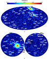 |
Fig. 1. Full-sky projections of the Compton-y signal encompassing the entire simulation volume in SLOW are shown in the following manner: (a) A full-sky projection in galactic coordinates. (b) On the left, the galactic northern sky is projected, while on the right, the galactic southern sky is shown. The zone of avoidance lies at the edge of the spheres. Circles are employed to mark the projected r500 values for the cross-identified clusters. Note that the cross-identification of A576 and A3571 was improved with respect to Dolag et al. (2023). |
4. Scaling relations for low redshift clusters
It has been extensively demonstrated that the subgrid model presented in Sect. 2.2 yields galaxy and ICM properties in galaxy clusters that closely align with observed trends and properties (Gupta et al. 2017; Singh et al. 2020). The Magneticum simulations employing the same hydrodynamical scheme, with a slightly earlier adaption of the galaxy formation treatment, have been compared to SZ data from Planck (Planck Collaboration XVI 2014) and SPT (McDonald et al. 2014). They have successfully replicated the observable X-ray luminosity relation (Biffi et al. 2013), among other ICM characteristics. In this context, we will test the results of our SLOW simulations to demonstrate their capability to reproduce SZ data and relationships with X-ray observables scaling relations.
Scaling relations are particularly interesting as they are tightly related to the physics of cluster formation and evolution. In the idealized framework where gravity is the dominant process in cluster evolution, self-similar models predict simple scaling relations between cluster properties, such as temperature, luminosity, and Compton-y value with total mass (Kaiser 1986). In general, these relations are described by power laws, around which some data points scatter according to a log-normal distribution. These relations describe positive correlations, so that largest systems have on average higher values of the correlated parameter. On top of this, as these relations come from the premise of self-similarity and thus gravity domination, any deviation of the relation may be a sign of important hydrodynamical processes taking center stage in the evolution history of these structures. Therefore, scaling relations are an important tool in cosmology as well as in the study of the thermodynamical history of clusters and their ICM.
We tested our simulated clusters scaling relations against the observed clusters scaling relations reported by Zhang et al. (2008), Pratt et al. (2009), Mantz et al. (2010a). The first three panels in Fig. 2 show the results of Lx – M500, Lx – Tx and Tx – M500 scaling relations for the clusters selections given in Pratt et al. (2009) in a redshift range of 0.05 < z < 0.164 (in red), Zhang et al. (2008) spanning the range 0.14 < z < 0.3 (in yellow) and Mantz et al. (2010a) containing clusters with z < 0.3 (in green). Even if this redshift threshold is small enough to keep evolution effects to a small level (Reichert et al. 2011), we corrected the data for possible redshift effects.
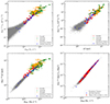 |
Fig. 2. Scaling relations within R500 for simulated clusters at z = 0 and for observed low redshift clusters. Gray data points represent the cluster values from our simulations, estimated using SUBFIND (Springel et al. 2001; Dolag et al. 2009; Saro et al. 2006). The clusters that have been cross-identified are highlighted in blue. Luminosity-mass (Lx – M500, top left), luminosity-temperature (Lx – kT, top right), temperature-mass (kT – M500, bottom left) panels show observational data from Pratt et al. (2009) (depicted as red points), which encompasses clusters with redshifts ranging from 0.05 to 0.164, Zhang et al. (2008) (depicted in yellow) with clusters spanning the redshift range of 0.14 to 0.3, and Mantz et al. (2010a) (depicted in green), which includes clusters with redshifts less than 0.3. The bottom right panel depicts the Compton-y – M500 scaling relation. For observational data in this case, we rely on Planck’s catalog PSZ1v2 (Planck Collaboration XXIX 2014), considering only clusters with a redshift of less than 0.1. |
We calculated the luminosities, temperatures, and masses for our clusters in the R500 radius using SUBFIND (Springel et al. 2001; Dolag et al. 2009; Saro et al. 2006). For the temperature, in order to focus on the ICM gas we performed a cutout above 105 K. The simulated data points for all clusters in our simulation are shown in gray, while the corresponding data points for our set of 46 clusters are plotted in blue. All three figures show a great agreement between the observed clusters and the simulated clusters in our box.
Furthermore, we examined the Compton-y – M500 relationship for our simulated clusters. In this instance, we selected observational data from the Planck database for clusters with redshifts below 0.1. For the simulated values, we generated Compton-y maps for each of the clusters in our simulations employing SMAC (Dolag et al. 2005a), and computed the total Compton-y emission within R500. Once more, our simulations faithfully reproduce the expected scaling relation presented in the observational data. Thus, we can conclude that our improved subgrid model presented in Sect. 2.2 can also successfully replicate the crucial ICM characteristics such as Lx – M500, Lx – Tx and Tx – M500 and Y500 – M500 scaling relations.
5. Results
5.1. Local cluster and their replicas in SLOW
Table A.1 presents a comparison of the positions of local clusters and their simulated counterparts. The median separation between the observed cluster position and that of its replica in our simulation is of 25 Mpc h−1, with only three exceeding a distance of 45 Mpc h−1.
During the cluster identification process based on observed positions, two primary sources of errors come into play. Firstly, when using distance measurements derived from redshift for the positions of our galaxy clusters, we encounter uncertainties associated with the peculiar velocity of the cluster. To quantify this uncertainty, we referred to the study by Dolag & Sunyaev (2013, Fig. 1), where the authors presented histograms of peculiar velocities of galaxy clusters in a cosmological box across different mass bins. We adopted the 1 sigma error values for each mass bin presented in Fig. 1 of the mentioned paper to illustrate the typical peculiar velocity uncertainties, which have a mild dependence on mass. These resulting uncertainty values are displayed in Col. 8 of Table A.1.
On the other hand, in simulations founded on peculiar velocities, uncertainties coming from distance moduli propagate to radial velocities and subsequently extend further to uncertainties on the reconstructed density and total velocity field. Consequently, uncertainties in the observed distances (which are of around a 20% of the distance value) are directly coupled with displacements of the three dimensional positions within the evolved simulation.
In addition, a positional error originates from the creation of the constraints for the initial conditions, where scales below the linear threshold are typically non-constrained. However, this generally adds an error of 3–4 Mpc, which is significantly smaller than the two errors discussed above.
Therefore the relative distances found for our simulated replicas, as presented in Table A.1, are reasonably small when compared to the above-discussed uncertainties, showing that we have a high-fidelity reproduction of these observed clusters in our simulation. Note that for half of the cluster replicas, the relative distances found are already almost fully covered when only considering the uncertainty of the observed cluster position based on their expected, typical peculiar velocity.
5.2. Detection significance
Originally, structure identification in reconstructions of the local Universe primarily relied on tracing the large-scale linear field (Hoffman 1993; Zaroubi et al. 1995; Fisher 1995; Bistolas & Hoffman 1998) More recently, reproductions based on simulations have shifted their focus toward individual, collapsed structures, leading to a manual one-to-one structure and galaxy cluster identification (e.g., Klypin et al. 2003; Dolag et al. 2004a; Carlesi et al. 2016b; Sorce 2018; Sorce et al. 2019, 2020, 2022). Recently, Pfeifer et al. (2023) extended this type of identification by associating well-defined probabilities to the cross-matched galaxy cluster pairs. Our current objective extends beyond the previous approach. We aim to identify collapsed, nonlinear structures at smaller scales within the larger-scale cosmological hydrodynamical box and assess their significance and the quality of their reproduction given the variety of multiwavelength observational data available for the individual galaxy clusters.
Therefore, once we have found counterparts for our galaxy cluster selection, we can consider the probability of such a finding compared to a random position in a very large simulation box. Here, we can take the relative distance from the observed position, the inferred mass of the galaxy cluster, or directly any observational signal that is typically used as a proxy for the cluster mass (like X-ray luminosity, temperature, etc.) directly into account.
In mathematical terms, we want to perform a hypothesis test, where we ask what is the p-value of our finding under the assumption of no difference compared to a null hypothesis, which in this case is a random simulation. This can give us a measure of how likely it is that our finding is in fact a product of the constraints in our ICs. Such a procedure is naturally only applicable for rare (e.g. relatively high-mass systems), but can be extended to smaller accompanying systems, see Seidel et al. (in prep.) for details. Particularly, we performed this test using the four main cluster properties that we considered throughout this paper, which are M500, Lx500, Tx500 and the Ysz500 signal. This time X-ray luminosities were also calculated using SMAC in the 0.1–2.5 keV band. We subsequently explain the procedure for M500, knowing that the analogous procedure applies to the rest of the properties.
The steps are the following:
-
We select bins for M500, ranging from 1014 M⊙ to 1015 M⊙ in steps of 10, giving a total amount of ten bins. Each of these bins will serve as a mass threshold for our cluster search.
-
We place a virtual observer at random positions in our cosmological box (a total of 1 million positions per mass bin), which is equivalent to positioning ourselves in a random box.
-
We choose each of these mass bins and use it as a threshold for the cluster property. Then we search in a radius around the random position of the first cluster which has a value for M500 larger than the threshold and we save this distance as our minimum radial distance. We perform this step using all bins as thresholds.
-
We compute a cumulative probability function for each of the mass bins, in order to calculate the one-tailored p-value for each cluster.
-
Now we study our selected clusters in the light of these cumulative probabilities. We take the relative positions of our clusters and perform a spline interpolation between the cumulative probabilities of all bins at a fixed radius. By doing this we are able to estimate the exact probability of each of our clusters in terms of the M500 value.
-
We calculate the significance of the match as 1–p, where p is the p-value associated with that cluster. The significance values for each cluster are listed in Table A.1.
Figures 3 and 4 depict the cumulative distribution functions representing various bins of our four central properties. In these figures, blue points signify the observed clusters, accompanied by their associated property uncertainties. Correspondingly, the simulated counterpart values are denoted in red. Apart from the mass uncertainty, we also need to consider the distance uncertainty originating from peculiar velocities, as well as distance moduli, as discussed in Sect. 5.1. Given the uncertainty in how the distance moduli errors affect our simulations, we have limited our analysis to the peculiar velocity uncertainty. For clarity, we have graphically represented this uncertainty as a red line only for five clusters at different relative distances: Coma, Centaurus, A3532, A2107, and A496. This uncertainty applies however to all represented clusters.
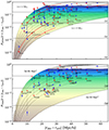 |
Fig. 3. Cumulative distribution functions for M500 and Y500, respectively. The top panel displays bins ranging from 1015 to 1014 M⊙, with increments of ten, showing the random expectation of finding a cluster of a certain mass or higher within a sphere whose radius corresponds to the distance displayed on the x-axis. Simulated M500 values, as estimated by SUBFIND, are represented in red. The blue data points represent the observed M500 values obtained from clusters Planck signals, including their associated errors. In cases where SZ-derived M500 values were unavailable, X-ray-derived M500 values were used (indicated by square points). For cluster A347 X-ray-derived mass information was not available, thus we used the M500 mass derived by converting the dynamical mass estimated by Tully. The observational uncertainties in the cluster’s position for Coma, A2734, AWM7, and Centaurus are represented by red lines, as an illustrative example of how such positional uncertainty can impact the results of the significance study (see Sect. 5.2 for a more comprehensive discussion). The bottom panel displays the cumulative distribution function for the SZ-derived signal in R500. Simulated datapoint values where estimated using SMAC (Dolag et al. 2005a). The bins range from 3 × 10⁻⁶ to 3 × 10⁻⁴ Mpc2, with increments of 2. |
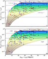 |
Fig. 4. Similar to Fig. 3, we show cumulative distribution functions for Lx and Tx within R500. For a better comparison with observations, we estimated the X-ray luminosity in the band 0.1–2.4 keV for every cluster using SMAC. In the top panel, the bin values range from 1044 erg × s−1 to 1045 erg × s−1, with increments of 10. Uneven spacing between higher-value bins has to do with the inherent limitations of small number statistics within our cosmological box (see Sect. 5.2 for a deeper discussion). The bottom panel presents the cumulative distribution function from the X-ray temperature in R500. We estimated this temperature using SUBFIND. The bin values range from 2 keV to 9 keV, with increments of 1 keV. |
Probability values below the −1σ threshold indicate a significance level exceeding 80%. Consequently, we classify all clusters falling below this threshold as highly significant matches. It is worth noting that the significance of these clusters can exhibit notable variations when considering distance errors. In the worst-case scenario, even with distance errors increasing the relative distance, the significance for highly significant clusters remains at higher than 50%. In contrast, under the best-case scenario, where the relative distance gets reduced, their significance can increase dramatically, surpassing the 99% mark.
Some of the lines for the values representing the higher-mass bins show unusual patterns, such as uneven spacing between bins or instances where two bins overlap. This is attributed to the inherent limitations of small number statistics within our cosmological box. As we move into higher property value ranges, the occurrence of clusters with such values diminishes. Nevertheless, it is important to note that these irregularities do not have any relevant impact on our significance estimate.
Lastly, we would like to emphasize the exceptionally high significance values observed across all properties for several pivotal local galaxy clusters, notably including Virgo, Coma, Centaurus, Perseus, Fornax, and Norma, among many others (see Table A.1). These significance values, hovering around 1.0, strongly indicate that the identification of these clusters is highly likely attributable to the constraints we have imposed, rather than being a random occurrence.
5.3. Properties’ comparison
A notable advantage of our constrained local Universe simulations lies in our ability to perform direct one-to-one comparisons once we have successfully matched our clusters with their simulated counterparts. Figure 5 illustrates the property ratios between observed and simulated structures, in relation to their relative distances. The data points are color-coded based on their significance, with higher significance levels represented by blue, while lower significance levels are denoted by yellow.
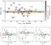 |
Fig. 5. Simulated and observed quantities’ ratios as a function of relative distance. (a) Ratio between the M500 mass, derived from the cluster SZ signal, and the SUBFIND-estimated M500 as a function of relative distance. The dotted line corresponds to the median of the distribution, while the shaded red region depicts the observed dispersion in the Compton-y–mass scaling relations (Planck Collaboration XI 2011). The three bottom panels present similar ratios for (b) X-ray luminosity (L500), (c) X-ray temperature (T500), (d) and SZ-signal (Y500). These data points are color-coded based on their mass significance, with higher significance levels indicated in black and lower significance levels denoted in yellow. |
In Fig. 5a, we illustrate the mass ratio of SZ effect-derived mass within R500 divided by the SUBFIND-estimated M500. The dashed line in the plot represents the median value of the data, while the red-shaded region surrounding the median corresponds to the dispersion observed in the Compton-y – M500 scaling relations (Planck Collaboration XI 2011, see Fig. 5). The median value is 0.87 indicating that the SZ effect-derived mass tends to be lower than the simulated mass. This finding aligns with estimates of the hydrostatic mass bias.
The hydrostatic mass bias is relevant for gas-derived mass estimations such as X-ray or SZ effect-derived masses, as it accounts for the fractional difference between the true mass and the cluster mass inferred using a gas proxy, assuming hydrostatic equilibrium. This bias is estimated from simulations to be between 10% and 20% (Lau et al. 2009, 2013; Biffi et al. 2016; Scheck et al. 2023). In simpler terms, ICM-based mass estimates tend to underestimate the actual mass by approximately a factor of 0.8–0.9, which closely matches the shift observed in the median of our mass ratios being (1 − b) = 0.87.
Furthermore, a majority of the clusters closely align with the median, and approximately half of them fall within the shaded region, which corresponds to the dispersion seen in the Compton-y – M500 scaling relation.
We also notice that Fig. 4a shows a greater dispersion among clusters matched at smaller relative distances, whereas the dispersion tends to be more confined to the proximity of the shaded region for clusters matched at larger relative distances. This observation highlights a potential bias in our matching process.
Our matching process relies in its first steps on positions and masses. In the search process, sometimes we find a very massive galaxy cluster very close to the target cluster’s observed position. This replica candidate has a high significance in terms of its mass as the relative distance between the observed and simulated cluster is small, pointing to the fact that its existence is very probably due to our constraints. Usually, after the complete selection procedure, that cluster will be selected as the corresponding cluster replica.
However, if we fail to identify a suitable counterpart in close proximity to the observed cluster, we expand our search radius. This broader search increases the pool of potential candidates for a match. Therefore, the probability of finding a candidate with a very similar mass to the observed one becomes higher at these extended distances. Thus, the mass scatter becomes lower for these clusters. These trends are only slightly reflected for temperatures, luminosities, and Compton-y (see Figs. 4b,c,d).
In light of these results, we would like to discuss the replication quality of the subset of extensively studied clusters in the literature listed in Table A.2.
Coma demonstrates excellent agreement in terms of mass. Its simulated mass of 9.61 × 10¹⁴ M⊙ aligns well with the X-ray derived mass of  , and it is just a bit higher than the SZ-derived mass. The simulated temperature of 7.06 keV also falls within the observed X-ray temperature range of 8.07 ± 0.29 keV. However, its luminosity and Compton-y values are higher by a factor of 1.5 and 3, respectively.
The Perseus cluster’s simulated mass of 5.17 × 10¹⁴ M⊙ is also in excellent agreement with its X-ray estimated mass of  . The simulated temperature of 4.97 keV closely matches the reported X-ray temperature of 6.42 ± 0.06 keV.
Virgo with a simulated M500 mass of 6.57 × 10¹⁴ M⊙ and a virial mass of 7.12 × 10¹⁴ M⊙, has a higher mass than the SZ estimated mass of 4.76 ± 0.55 × 10¹⁴ M⊙. However, considering various studies over recent years estimating Virgo’s virial mass in the range of 6.0–8.0 × 10¹⁴ M⊙, like de Vaucouleurs (1960), Karachentsev et al. (2014) at 8.0 ± 2.3 ×10¹⁴ M⊙, and Kashibadze et al. (2020) at 6.3 ± 0.9 ×10¹⁴ M⊙, (see Table 3 in Lebeau et al. 2024, for a longer list), we still view the Virgo cluster’s mass in the simulation as accurately reproduced.
Hydra also agrees in its mass estimation, with 2.64 × 10¹⁴ M⊙ in the simulation and  given by the X-ray observation. The temperature value lies also very close, from 3.37 keV in the simulation to 3.15 ± 0.05 keV from observations. It is important to note that these clusters have different dynamical states and likely underwent different formation paths, as discussed in Sect. 3.1
Clusters’ replicas for Centaurus, AWM7, Fornax, and Norma deviate more from the observed quantities than the previously mentioned cluster replica. One key factor contributing to these differences in replication quality is the cluster’s position in the sky. If we examine the positions of Centaurus, AWM7, Fornax, and Norma, we find that they are located in close proximity to the “Zone of Avoidance” (as seen in Fig. 1), where the extinction is severe. Consequently, the quality and quantity of observational data available for our constraints can be more limited. Perseus and Hydra, on the other hand, are better reproduced, even though they are near the Zone of Avoidance demonstrating the power of using peculiar velocities, which by tracing the potential can put constraints far beyond their actual sampling points.
Compared to other simulations of the local volume constrained with galaxy distributions such as SIBELIUS-DARK (McAlpine et al. 2022), we observe that the significant improvement in the replication of crucial clusters like Perseus and Virgo (Sorce 2018) can now be extended to various other local clusters. For instance, Perseus, with an observed X-ray-derived M500 of 6.08 × 10¹⁴ M⊙, was previously simulated with a mass of 1.87 × 10¹⁵ M⊙ in SIBELIUS-DARK, whereas our replication yielded a closer mass of 5.17 × 10¹⁴ M⊙. Similarly for Virgo, its 6.57 × 10¹⁴ M⊙ mass in our simulation lies in the range of 6 − 8 × 10¹⁴ M⊙ reported in the previous mentioned studies by de Vaucouleurs (1960), Karachentsev et al. (2014) and Kashibadze et al. (2020), while SIBELIUS-DARK contained a replica with a lower mass of 2.7 × 10¹⁴ M⊙ in R500 and 3.5 × 10¹⁴ M⊙ in R200. Hydra replica is now also better reproduced in terms of mass, as we find a cluster replica with a mass of 2.6 × 10¹⁴ M⊙, lying very well within the observed X-ray derived mass range of  , in contrast to the 3.5 × 10¹⁴ M⊙ mass value reported in SIBELIUS-DARK (see Table B1 in McAlpine et al. 2022, for comparison). Indeed, when having a closer look at the quantity ratios in Fig. 5, we see that the general mass scatter is low, pointing to a generally good cluster reproduction.
In this context, the cases of Norma and Centaurus are particularly intriguing, as they stand out as outliers in the panels depicted in Fig. 5. Specifically, in the case of Norma, the simulated mass is approximately six times lower than the observed mass. As mentioned earlier, the proximity of the Norma cluster to the zone of avoidance and its association with the “Great Attractor” result in poorly constrained information about its mass and nature (Lynden-Bell et al. 1988; Woudt et al. 2007). In addition, Norma exhibits an elongated structure in both observations (as seen in Woudt et al. 2007) and our simulation. This characteristic may indicate a highly dynamic, accreting structure, further complicating the estimation of its true mass.
Norma shares its region of the sky with Hydra, Centaurus, and the Shapley clusters. Hydra and Centaurus form a cluster pair in the southern sky, positioned closer to us than Norma. While these two clusters are less massive, they are believed to play a central role in shaping the “Great Attractor” structure (Raychaudhury 1989). The challenge lies in their lower mass and their sky location, making it difficult to obtain high-quality observational data for accurate replication.
However, it is worth noting that the mass of Hydra is well reproduced, lying within the error region estimated from X-ray observations. The Centaurus cluster replica lies in the high mass end of the observed masses for this cluster. Indeed, its mass is 1.18 times higher than the dynamically estimated mass. Both structures if observed combined, constitute a good replica of the Centaurus – Hydra pair. When considering the observed X-ray mass for Hydra (2.5 × 10¹⁴ M⊙) and the SZ-effect and dynamical derived masses for Centaurus (1.23 × 10¹⁴ M⊙ and 5.28 × 10¹⁴ M⊙), the total pair mass falls within the range of 3.73 × 10¹⁴ to 7.78 × 10¹⁴ M⊙. In our simulation, the combined mass of both clusters amounts to 8.85 × 10¹⁴ M⊙, which lies only slightly higher than the observed range. Additionally, Fig. 6 depicts a density map of the Centaurus-Hydra region, with overlaid positions of observed galaxies. Galaxies directly assigned to the Hydra and Centaurus clusters are marked in red, while those in the surrounding region are in orange. This figure illustrates our ability to accurately reproduce the relative positions of Centaurus and Hydra, as well as the structure of the surrounding cosmic web. Even more, evolving the local Universe forward in time as presented by Seidel et al. (in prep.) shows that the Centaurus-Hydra pair merge. This indicates that although the individual clusters are less well replicated, the overall collapsing structure associated with them is well reproduced.
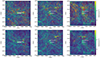 |
Fig. 6. Density map of the Centaurus-Hydra region in the SLOW simulation, presented in supergalactic coordinates and created using SMAC. The locations of the Centaurus and Hydra clusters are marked with two white circles, each indicating the R500 radius of the respective structures. In the top panels, observed galaxies from the 2MRS1175 North Groups catalog associated with Centaurus and Hydra are highlighted in red. Additionally, galaxies listed in both the 2MRS1175 North and South Groups catalogs are shown in orange. These galaxy positions have been corrected to account for distortions such as the “fingers of god” effect. In the bottom panels, all galaxies from the CF-2 Catalog in this area are displayed in orange, with those attributed to Centaurus and Hydra in red, without adjusting for the “fingers of god” correction. |
In conclusion, our simulations provide valuable insights into the properties of numerous key local galaxy clusters. However, there remains room for improvement, especially in accurately replicating even more clusters as well as structures situated near the zone of avoidance, where observational data is limited and replication could possibly be improved by the selection of certain, random realizations.
Improving the precision of these simulations poses several challenges: acquiring more comprehensive data, including currently sparsely sampled regions, refining the galaxy formation physics treatment within the simulations as well as improving observational mass estimates for better evaluation of similarity between simulated and observed clusters. Such improvements will be essential for gaining a deeper understanding of these complex sky regions.
5.4. Observational tracers’ reliability
As previously discussed in the preceding sections, it is important to acknowledge the presence of observational errors and biases, which can at times be challenging to precisely quantify. One of our central observational parameters is mass estimations. It is noteworthy that these different mass estimation approaches yield significant discrepancies in their mass assessments for various clusters.
A potential source of bias in mass estimation appears to be the distance of the clusters from the observer. To explore this possibility, we conducted tests to assess the behavior of each mass estimation method in relation to distance. Initially, we conducted this analysis with respect to the simulated masses. Figure 7 illustrates the relationship between observed mass estimates and simulated masses in relation to distance. We categorized the clusters into two sets, one with closer members and the other with more distant members, each with an equal number of clusters. The median of both sets is represented by a green dashed line, while the green shaded region delineates the range encompassing 50% of the clusters above and below the median.
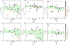 |
Fig. 7. Mass ratios as a function of total distance. The top figures present the mass ratio between SUBFIND-estimated M500 and three different mass estimations: (a) M500 derived from the dynamical mass as provided in the Tully galaxy group catalog (Tully 2015): Mdyn, (b) M500 derived from SZ measurements as available in the Planck database: MSZ, and (c) M500 derived from X-ray observations: Mxray. These ratios are plotted against the total distance of the cluster. In addition, the bottom figures illustrate the ratios between various observational mass estimations: (d) Msz/Mdyn, (e) Mxray/Mdyn, and (f) Msz/Mxray, all in relation to the total distance of the cluster. (For further details on the observed quantities, please refer to Table A.2). A vertical dashed line divides the clusters into two sets with an equal number of clusters. The green horizontal lines represent the median values for each set, while the green shaded regions indicate the range that encompasses 50% of the clusters above and below the median. |
Masses derived from X-ray emissions (Fig. 7b) and the SZ effect (Fig. 7c) exhibit minimal scatter around the median for both the closer and more distant cluster sets. The scatter shows no significant increase or decrease with cluster distance in these cases. In contrast, the scenario is quite different for dynamical masses (Fig. 7a), where the scatter notably increases for clusters at greater distances.
Furthermore, we conducted comparative analyses among the various mass estimation methods while considering their relationship with distance, as depicted in Figs. 7d–f. When comparing dynamical masses against X-ray and SZ-effect derived mass estimations, dynamical masses consistently display a high scatter, which becomes even more pronounced for clusters located farther away, mirroring the pattern observed in Fig. 7a. Conversely, the scatter between X-ray and SZ-effect derived mass estimations is significantly low, as evident in Fig. 7f. Nevertheless, the scatter between different observed mass estimates is as large as the scatter between simulated and observed cluster counterparts. Taken together, this points to the fact that the level at which the constrained simulation reproduces the mass of the local galaxy clusters is at the level of the uncertainties in the observational mass estimates.
6. Summary and conclusions
In this paper, we have presented the first results on cluster identification in our constrained, hydrodynamical cosmological simulation of the local Universe (SLOW), which includes cooling, star formation, and the evolution of super-massive black holes. We compiled a dataset of over 221 observed galaxy clusters and groups within the local volume covered by our simulation from existing literature, collecting X-ray luminosities, temperatures, and Compton-y signals as well as inferred masses of these systems, when available. From this sample, we cross-identified 46 halos in the simulation, which are candidates to represent the according galaxy clusters within the local Universe. We then computed the significance of these associations based on different observables and compared the global properties between the observed and simulated counterparts.
-
The galaxy clusters within the simulation generally follow the observed scaling relations between mass, temperature, X-ray luminosity, and SZ signal. This has allowed us for the first time to evaluate the cross identification between simulations and observations not only on the total mass but also directly on the full band width of observational signals from the ICM. Thereby such direct comparisons avoid the various biases inherited within the different methods to determine the total mass of galaxy clusters from observational proxies.
-
We compared the positions of cross-identified galaxy clusters between observations and simulations combined with the match of their various global properties (e.g., mass, total X-ray luminosity, temperature, or SZ signal) and computed the probability of finding a similar match in a random position within a large volume simulation. From this, we computed a significance of the match against the null hypothesis obtained from a random simulation volume.
-
This sample of clusters encompasses the 13 most massive clusters with a M500 exceeding 2 × 10¹⁴ M⊙, as identified by the SZ signal from Planck observations within a radius of approximately 300 Mpc. This highlights the success of our constrained simulation in precisely replicating the local galaxy clusters.
-
Based on the assessment of the significance of a match, only a small fraction cannot be distinguished from a random selection. On the contrary, even 18 of the matched clusters exhibited significance values exceeding 0.8 across all studied quantities. Notably, Virgo, Coma, and Perseus achieved a significance very close to 1.0 for all quantities with the smallest value being 0.98.
-
Compared to other constrained simulations, we report a significant improvement in the number of identified replicas of crucial galaxy clusters in the local Universe, where masses now agree with their observational counterparts. Even for very prominent clusters such as Perseus, Virgo, and Hydra, we noticed that compared to simulations where the constraints are based on galaxy distributions, such as SIBELIUS-DARK, the mass is recovered better by the SLOW simulation.
-
We also investigated the impact of the observational distance uncertainty on our comparison. For the matched sample of galaxy clusters, the inferred displacement between the position in our simulation and the cluster position based on the observed redshift often reflects the uncertainties induced by the unknown peculiar velocity of the clusters. In the majority of cases, this displacement is smaller than the typical error in the distance modulus of the individual galaxies used for constructing the constraints for the initial condition. This assessment further demonstrates that our constrained simulation of the local Universe reproduces a large number of galaxy clusters that can be directly compared with their observational counterpart.
-
Comparing the X-ray luminosity and temperature between observations and the simulated counterparts, the obtained width of the relative scatter is 1.7 and 1.5, respectively, for 68% of the clusters. For the SZ signal, this scatter is of a factor 2.1. Interestingly, when comparing the sample median of the M500 obtained from the simulations with the observed one inferred from the SZ signal, we would deduce a bias of (1 − b) = 0.87, which is in the range predicted by other simulations.
-
With our sample of cross-identified clusters, we compared the masses of the simulated and observed clusters using mass estimates based on different observables (this being: the SZ-effect derived mass, dynamical masses from Tully’s galaxy catalog, and X-ray signal derived masses). We find that the scatter between different observed mass estimates is as large as the scatter between simulated and observed cluster counterparts. We neither find any strong correlation of the scatter with the distance of the cluster, nor with the significance assessment, except a tendency of the observational-inferred dynamical mass to have a higher scatter at larger distances with respect to other measurements as well as with respect to the simulations. Overall this indicates that the level in which the constrained simulation is reproducing the mass of the local galaxy clusters is at the level of the uncertainties of the observational mass estimates.
Overall, the current SLOW simulation of the local Universe faithfully replicates numerous fundamental characteristics for a sizable number of galaxy clusters within our local neighborhood. This is a first step in establishing an exciting avenue for cluster and cosmological research, where such simulations enable us to investigate the formation and evolution of individual galaxy clusters. This will allow us to study the physical processes governing the formation and evolution of galaxy clusters beyond the limitations inherited when using averaged populations toward marking the transition to test the effect of individual formation histories and environments.
It can though be shown that some small scales are induced by the large-scale environment. Carlesi et al. (2016a) showed that it is the case of the local Group.
Acknowledgments
We want to thank I. Khabibullin for his help and insightful comments on the X-ray-derived data appearing in our data tables. The authors also thank the comments and discussions with all the members of this project. They thank the Center for Advanced Studies (CAS) of LMU Munich for hosting the collaborators of the LOCALIZATION project for a week-long workshop. This work was supported by the grant agreements ANR-21-CE31-0019/490702358 from the French Agence Nationale de la Recherche/DFG for the LOCALIZATION project. NA acknowledges support from the European Union’s Horizon 2020 research and innovation program grant agreement ERC-2015-AdG 695561 (ByoPiC, https://byopic.eu). KD and MV acknowledge support by the Excellence Cluster ORIGINS which is funded by the Deutsche Forschungsgemeinschaft (DFG, German Research Foundation) under Germany’s Excellence Strategy – EXC-2094 – 390783311 and funding for the COMPLEX project from the European Research Council (ERC) under the European Union’s Horizon 2020 research and innovation program grant agreement ERC-2019-AdG 882679. MV is supported by the Fondazione ICSC National Recovery and Resilience Plan (PNRR), Project ID CN-00000013 “Italian Research Center on High-Performance Computing, Big Data and Quantum Computing” funded by MUR – Next Generation EU. MV also acknowledges partial financial support from the INFN Indark Grant. The calculations for the hydro-dynamical simulations were carried out at the Leibniz Supercomputer Center (LRZ) under the project pn68na. We are especially grateful for the support by M. Petkova through the Computational Center for Particle and Astrophysics (C2PAP).
References
- Abazajian, K., Adelman-McCarthy, J. K., Agüeros, M. A., et al. 2003, AJ, 126, 2081 [Google Scholar]
- Abazajian, K. N., Adelman-McCarthy, J. K., Agüeros, M. A., et al. 2009, ApJS, 182, 543 [Google Scholar]
- Aharonian, F. A., Akamatsu, H., Akimoto, F., et al. 2017, ApJ, 837, L15 [NASA ADS] [CrossRef] [Google Scholar]
- Allen, S. W., Fabian, A. C., Johnstone, R. M., et al. 1993, MNRAS, 262, 901 [NASA ADS] [CrossRef] [Google Scholar]
- Andrade-Santos, F., Nulsen, P. E. J., Kraft, R. P., et al. 2013, ApJ, 766, 107 [NASA ADS] [CrossRef] [Google Scholar]
- Angulo, R. E., Springel, V., White, S. D. M., et al. 2012, MNRAS, 426, 2046 [NASA ADS] [CrossRef] [Google Scholar]
- Applegate, D. E., Mantz, A., Allen, S. W., et al. 2016, MNRAS, 457, 1522 [NASA ADS] [CrossRef] [Google Scholar]
- Arnaud, M., Aghanim, N., Gastaud, R., et al. 2001, A&A, 365, L67 [NASA ADS] [CrossRef] [EDP Sciences] [Google Scholar]
- Balogh, M. L., Baldry, I. K., Nichol, R., et al. 2004, ApJ, 615, L101 [Google Scholar]
- Beck, A. M., Murante, G., Arth, A., et al. 2015, MNRAS, 455, 2110 [Google Scholar]
- Biffi, V., Dolag, K., & Böhringer, H. 2013, MNRAS, 428, 1395 [Google Scholar]
- Biffi, V., Borgani, S., Murante, G., et al. 2016, ApJ, 827, 112 [NASA ADS] [CrossRef] [Google Scholar]
- Binggeli, B., & Huchra, J. 2000, Encyclopedia of Astronomy and Astrophysics, ed. P. Murdin, 1822 [Google Scholar]
- Bistolas, V., & Hoffman, Y. 1998, ApJ, 492, 439 [NASA ADS] [CrossRef] [Google Scholar]
- Biviano, A. 1998, in Untangling Coma Berenices: A New Vision of an Old Cluster, eds. A. Mazure, F. Casoli, F. Durret, & D. Gerbal [Google Scholar]
- Biviano, A., Durret, F., Gerbal, D., et al. 1996, A&A, 311, 95 [NASA ADS] [Google Scholar]
- Böhringer, H., Voges, W., Fabian, A. C., Edge, A. C., & Neumann, D. M. 1993, MNRAS, 264, L25 [NASA ADS] [CrossRef] [Google Scholar]
- Böhringer, H., Chon, G., & Kronberg, P. P. 2016, A&A, 596, A22 [NASA ADS] [CrossRef] [EDP Sciences] [Google Scholar]
- Böss, L. M., Dolag, K., Steinwandel, U. P., et al. 2023, A&A, submitted [arXiv:2310.13734] [Google Scholar]
- Branduardi-Raymont, G., Fabricant, D., Feigelson, E., et al. 1981, ApJ, 248, 55 [CrossRef] [Google Scholar]
- Briel, U. G., Henry, J. P., Lumb, D. H., et al. 2001, A&A, 365, L60 [NASA ADS] [CrossRef] [EDP Sciences] [Google Scholar]
- Carlesi, E., Hoffman, Y., Sorce, J. G., & Gottlöber, S. 2016a, MNRAS, 465, 4886 [Google Scholar]
- Carlesi, E., Sorce, J. G., Hoffman, Y., et al. 2016b, MNRAS, 458, 900 [NASA ADS] [CrossRef] [Google Scholar]
- Chen, Y., Reiprich, T. H., Böhringer, H., Ikebe, Y., & Zhang, Y.-Y. 2007, A&A, 466, 805 [NASA ADS] [CrossRef] [EDP Sciences] [Google Scholar]
- Chen, K.-F., Oguri, M., Lin, Y.-T., & Miyazaki, S. 2020, ApJ, 891, 139 [NASA ADS] [CrossRef] [Google Scholar]
- Chiu, I. N., Klein, M., Mohr, J., & Bocquet, S. 2023, MNRAS, 522, 1601 [NASA ADS] [CrossRef] [Google Scholar]
- Colless, M., Dalton, G., Maddox, S., et al. 2001, MNRAS, 328, 1039 [Google Scholar]
- Courtois, H. M., Hoffman, Y., Tully, R. B., & Gottlöber, S. 2012, ApJ, 744, 43 [NASA ADS] [CrossRef] [Google Scholar]
- Courtois, H. M., Pomarède, D., Tully, R. B., Hoffman, Y., & Courtois, D. 2013, AJ, 146, 69 [NASA ADS] [CrossRef] [Google Scholar]
- Dark Energy Survey Collaboration (Abbott, T., et al.) 2016, MNRAS, 460, 1270 [Google Scholar]
- de Haan, T., Benson, B. A., Bleem, L. E., et al. 2016, ApJ, 832, 95 [NASA ADS] [CrossRef] [Google Scholar]
- de Vaucouleurs, G. 1960, ApJ, 131, 585 [NASA ADS] [CrossRef] [Google Scholar]
- Dolag, K., & Sunyaev, R. 2013, MNRAS, 432, 1600 [NASA ADS] [CrossRef] [Google Scholar]
- Dolag, K., Grasso, D., Springel, V., & Tkachev, I. 2004a, Sov. J. Exp. Theor. Phys. Lett., 79, 583 [NASA ADS] [CrossRef] [Google Scholar]
- Dolag, K., Jubelgas, M., Springel, V., Borgani, S., & Rasia, E. 2004b, ApJ, 606, L97 [NASA ADS] [CrossRef] [Google Scholar]
- Dolag, K., Hansen, F. K., Roncarelli, M., & Moscardini, L. 2005a, MNRAS, 363, 29 [Google Scholar]
- Dolag, K., Vazza, F., Brunetti, G., & Tormen, G. 2005b, MNRAS, 364, 753 [NASA ADS] [CrossRef] [Google Scholar]
- Dolag, K., Borgani, S., Murante, G., & Springel, V. 2009, MNRAS, 399, 497 [Google Scholar]
- Dolag, K., Komatsu, E., & Sunyaev, R. 2016, MNRAS, 463, 1797 [Google Scholar]
- Dolag, K., Sorce, J. G., Pilipenko, S., et al. 2023, A&A, 677, A169 [NASA ADS] [CrossRef] [EDP Sciences] [Google Scholar]
- Donnert, J., Dolag, K., Brunetti, G., Cassano, R., & Bonafede, A. 2010, MNRAS, 401, 47 [NASA ADS] [CrossRef] [Google Scholar]
- Doumler, T., Courtois, H., Gottlöber, S., & Hoffman, Y. 2013a, MNRAS, 430, 902 [NASA ADS] [CrossRef] [Google Scholar]
- Doumler, T., Gottlöber, S., Hoffman, Y., & Courtois, H. 2013b, MNRAS, 430, 912 [NASA ADS] [CrossRef] [Google Scholar]
- Doumler, T., Hoffman, Y., Courtois, H., & Gottlöber, S. 2013c, MNRAS, 430, 888 [NASA ADS] [CrossRef] [Google Scholar]
- Dubois, Y., Peirani, S., Pichon, C., et al. 2016, MNRAS, 463, 3948 [Google Scholar]
- Dupuy, A., & Courtois, H. M. 2023, A&A, 678, A176 [NASA ADS] [CrossRef] [EDP Sciences] [Google Scholar]
- Eckert, D., Molendi, S., & Paltani, S. 2011, A&A, 526, A79 [NASA ADS] [CrossRef] [EDP Sciences] [Google Scholar]
- Eckert, D., Gaspari, M., Gastaldello, F., Le Brun, A. M. C., & O’Sullivan, E. 2021, Universe, 7, 142 [NASA ADS] [CrossRef] [Google Scholar]
- Fabian, A. C., Iwasawa, K., Reynolds, C. S., & Young, A. J. 2000, PASP, 112, 1145 [NASA ADS] [CrossRef] [Google Scholar]
- Fabian, A. C., Sanders, J. S., Allen, S. W., et al. 2011, MNRAS, 418, 2154 [Google Scholar]
- Fabjan, D., Borgani, S., Tornatore, L., et al. 2010, MNRAS, 401, 1670 [Google Scholar]
- Fisher, K. 1995, MNRAS, 272, 705 [NASA ADS] [CrossRef] [Google Scholar]
- Fitchett, M., & Webster, R. 1987, ApJ, 317, 653 [Google Scholar]
- Frenk, C., & White, S. 2012, Ann. Phys., 524, 507 [NASA ADS] [CrossRef] [Google Scholar]
- Garrison-Kimmel, S., Boylan-Kolchin, M., Bullock, J. S., & Lee, K. 2014, MNRAS, 438, 2578 [NASA ADS] [CrossRef] [Google Scholar]
- Garrison-Kimmel, S., Hopkins, P. F., Wetzel, A., et al. 2019, MNRAS, 487, 1380 [NASA ADS] [CrossRef] [Google Scholar]
- Gruen, D., Seitz, S., Brimioulle, F., et al. 2014, MNRAS, 442, 1507 [CrossRef] [Google Scholar]
- Gupta, N., Saro, A., Mohr, J. J., Dolag, K., & Liu, J. 2017, MNRAS, 469, 3069 [Google Scholar]
- Hirschmann, M., Dolag, K., Saro, A., et al. 2014, MNRAS, 442, 2304 [Google Scholar]
- Hoekstra, H., Herbonnet, R., Muzzin, A., et al. 2015, MNRAS, 449, 685 [NASA ADS] [CrossRef] [Google Scholar]
- Hoffman, Y. 1993, in Cosmic Velocity Fields, Proceedings of the 9th IAP Astrophysics Meeting, Institut d’Astrophysique, eds. F. R. Bouchet & M. Lachièze-Rey (Gif-sur-Yvette: Editions Frontieres), 357 [Google Scholar]
- Hoffman, Y., & Ribak, E. 1991, ApJ, 380, L5 [NASA ADS] [CrossRef] [Google Scholar]
- Hoffman, Y., & Ribak, E. 1992, ApJ, 384, 448 [NASA ADS] [CrossRef] [Google Scholar]
- Hurier, G., & Angulo, R. E. 2018, A&A, 610, L4 [NASA ADS] [CrossRef] [EDP Sciences] [Google Scholar]
- Ider Chitham, J., Comparat, J., Finoguenov, A., et al. 2020, MNRAS, 499, 4768 [NASA ADS] [CrossRef] [Google Scholar]
- Ikebe, Y., Reiprich, T. H., Böhringer, H., Tanaka, Y., & Kitayama, T. 2002, A&A, 383, 773 [NASA ADS] [CrossRef] [EDP Sciences] [Google Scholar]
- Jasche, J., & Lavaux, G. 2019, A&A, 625, A64 [NASA ADS] [CrossRef] [EDP Sciences] [Google Scholar]
- Jimeno, P., Diego, J. M., Broadhurst, T., Martino, I. D., & Lazkoz, R. 2018, MNRAS, 478, 638 [NASA ADS] [CrossRef] [Google Scholar]
- Kaiser, N. 1986, MNRAS, 222, 323 [Google Scholar]
- Kaplan, D. E., Luty, M. A., & Zurek, K. M. 2009, Phys. Rev. D, 79, 115016 [NASA ADS] [CrossRef] [Google Scholar]
- Kapteyn, J. C. 1914, ApJ, 40, 187 [CrossRef] [Google Scholar]
- Karachentsev, I. D., Tully, R. B., Wu, P.-F., Shaya, E. J., & Dolphin, A. E. 2014, ApJ, 782, 4 [NASA ADS] [CrossRef] [Google Scholar]
- Kashibadze, O. G., Karachentsev, I. D., & Karachentseva, V. E. 2020, A&A, 635, A135 [NASA ADS] [CrossRef] [EDP Sciences] [Google Scholar]
- Kim, J.-H., Abel, T., Agertz, O., et al. 2014, ApJS, 210, 14 [Google Scholar]
- Klypin, A., Hoffman, Y., Kravtsov, A. V., & Gottlöber, S. 2003, ApJ, 596, 19 [NASA ADS] [CrossRef] [Google Scholar]
- Klypin, A. A., Trujillo-Gomez, S., & Primack, J. 2011, ApJ, 740, 102 [NASA ADS] [CrossRef] [Google Scholar]
- Kollmeier, J., Anderson, S. F., Blanc, G. A., et al. 2019, Bull. Am. Astron. Soc., 51, 274 [Google Scholar]
- Kravtsov, A. V., & Borgani, S. 2012, ARA&A, 50, 353 [Google Scholar]
- Kravtsov, A. V., Klypin, A., & Hoffman, Y. 2002, ApJ, 571, 563 [NASA ADS] [CrossRef] [Google Scholar]
- Landy, S. D., & Szalay, A. S. 1992, ApJ, 391, 494 [NASA ADS] [CrossRef] [Google Scholar]
- Lau, E. T., Kravtsov, A. V., & Nagai, D. 2009, ApJ, 705, 1129 [NASA ADS] [CrossRef] [Google Scholar]
- Lau, E. T., Nagai, D., & Nelson, K. 2013, ApJ, 777, 151 [NASA ADS] [CrossRef] [Google Scholar]
- Lebeau, T., Sorce, J. G., Aghanim, N., Hernández-Martínez, E., & Dolag, K. 2024, A&A, 682, A157 [NASA ADS] [CrossRef] [EDP Sciences] [Google Scholar]
- Libeskind, N. I., Carlesi, E., Grand, R. J. J., et al. 2020, MNRAS, 498, 2968 [NASA ADS] [CrossRef] [Google Scholar]
- Lynden-Bell, D., Faber, S. M., Burstein, D., et al. 1988, ApJ, 326, 19 [NASA ADS] [CrossRef] [Google Scholar]
- Malavasi, N., Sorce, J. G., Dolag, K., & Aghanim, N. 2023, A&A, 675, A76 [NASA ADS] [CrossRef] [EDP Sciences] [Google Scholar]
- Malmquist, K. G. 1922, Meddelanden fran Lunds Astronomiska Observatorium Serie I, 100, 1 [Google Scholar]
- Mantz, A., Allen, S. W., Ebeling, H., Rapetti, D., & Drlica-Wagner, A. 2010a, MNRAS, 406, 1773 [NASA ADS] [Google Scholar]
- Mantz, A., Allen, S. W., Rapetti, D., & Ebeling, H. 2010b, MNRAS, 406, 1759 [NASA ADS] [Google Scholar]
- Mantz, A. B., von der Linden, A., Allen, S. W., et al. 2015, MNRAS, 446, 2205 [Google Scholar]
- Mathis, H., Lemson, G., Springel, V., et al. 2002, MNRAS, 333, 739 [NASA ADS] [CrossRef] [Google Scholar]
- McAlpine, S., Helly, J. C., Schaller, M., et al. 2022, MNRAS, 512, 5823 [CrossRef] [Google Scholar]
- McDonald, M., Benson, B. A., Vikhlinin, A., et al. 2013, ApJ, 774, 23 [NASA ADS] [CrossRef] [Google Scholar]
- McDonald, M., Benson, B. A., Vikhlinin, A., et al. 2014, ApJ, 794, 67 [Google Scholar]
- Medezinski, E., Oguri, M., Nishizawa, A. J., et al. 2018, PASJ, 70, 30 [NASA ADS] [Google Scholar]
- Meissner, K. A., & Nicolai, H. 2019, Phys. Rev. D, 100, 035001 [NASA ADS] [CrossRef] [Google Scholar]
- Mellier, Y., Mathez, G., Mazure, A., Chauvineau, B., & Proust, D. 1988, A&A, 199, 67 [NASA ADS] [Google Scholar]
- Neumann, D. M., Arnaud, M., Gastaud, R., et al. 2001, A&A, 365, L74 [NASA ADS] [CrossRef] [EDP Sciences] [Google Scholar]
- Nurgaliev, D., McDonald, M., Benson, B. A., et al. 2017, ApJ, 841, 5 [Google Scholar]
- Ocvirk, P., Aubert, D., Sorce, J. G., et al. 2020, MNRAS, 496, 4087 [NASA ADS] [CrossRef] [Google Scholar]
- Okabe, N., & Smith, G. P. 2016, MNRAS, 461, 3794 [Google Scholar]
- Olchanski, M., & Sorce, J. G. 2018, A&A, 614, A102 [NASA ADS] [CrossRef] [EDP Sciences] [Google Scholar]
- Overzier, R. A. 2016, A&ARv., 24, 1 [NASA ADS] [CrossRef] [Google Scholar]
- Pacaud, F., Pierre, M., Melin, J. B., et al. 2018, A&A, 620, A10 [NASA ADS] [CrossRef] [EDP Sciences] [Google Scholar]
- Pfeifer, S., Valade, A., Gottlöber, S., et al. 2023, MNRAS, 523, 5985 [NASA ADS] [CrossRef] [Google Scholar]
- Piffaretti, R., & Valdarnini, R. 2008, A&A, 491, 71 [NASA ADS] [CrossRef] [EDP Sciences] [Google Scholar]
- Pillepich, A., Springel, V., Nelson, D., et al. 2018, MNRAS, 473, 4077 [Google Scholar]
- Planck Collaboration XI. 2011, A&A, 536, A11 [NASA ADS] [CrossRef] [EDP Sciences] [Google Scholar]
- Planck Collaboration XVI. 2014, A&A, 571, A16 [NASA ADS] [CrossRef] [EDP Sciences] [Google Scholar]
- Planck Collaboration XXIX. 2014, A&A, 571, A29 [NASA ADS] [CrossRef] [EDP Sciences] [Google Scholar]
- Planck Collaboration Int. X. 2013, A&A, 554, A140 [NASA ADS] [CrossRef] [EDP Sciences] [Google Scholar]
- Planck Collaboration Int. XL. 2016, A&A, 596, A101 [EDP Sciences] [Google Scholar]
- Prada, F., Klypin, A. A., Cuesta, A. J., Betancort-Rijo, J. E., & Primack, J. 2012, MNRAS, 423, 3018 [NASA ADS] [CrossRef] [Google Scholar]
- Pratt, G. W., Croston, J. H., Arnaud, M., & Böhringer, H. 2009, A&A, 498, 361 [NASA ADS] [CrossRef] [EDP Sciences] [Google Scholar]
- Ragagnin, A., Saro, A., Singh, P., & Dolag, K. 2021, MNRAS, 500, 5056 [Google Scholar]
- Raychaudhury, S. 1989, Nature, 342, 251 [NASA ADS] [CrossRef] [Google Scholar]
- Reichert, A., Böhringer, H., Fassbender, R., & Mühlegger, M. 2011, A&A, 535, A4 [NASA ADS] [CrossRef] [EDP Sciences] [Google Scholar]
- Saintonge, A. 2007, AJ, 133, 2087 [NASA ADS] [CrossRef] [Google Scholar]
- Saro, A., Borgani, S., Tornatore, L., et al. 2006, MNRAS, 373, 397 [NASA ADS] [CrossRef] [Google Scholar]
- Sawala, T., Frenk, C. S., Fattahi, A., et al. 2016, MNRAS, 457, 1931 [Google Scholar]
- Schaye, J., Crain, R. A., Bower, R. G., et al. 2015, MNRAS, 446, 521 [Google Scholar]
- Scheck, D., Sanders, J. S., Biffi, V., et al. 2023, A&A, 670, A33 [NASA ADS] [CrossRef] [EDP Sciences] [Google Scholar]
- Schellenberger, G., & Reiprich, T. H. 2017, MNRAS, 471, 1370 [Google Scholar]
- Schwarz, H. E., Corradi, R. L. M., & Melnick, J. 1992, A&AS, 96, 23 [NASA ADS] [Google Scholar]
- Sereno, M., & Ettori, S. 2017, MNRAS, 468, 3322 [CrossRef] [Google Scholar]
- Shang, C., & Scharf, C. 2008, ApJ, 690, 879 [Google Scholar]
- Simionescu, A., Werner, N., Urban, O., et al. 2012, ApJ, 757, 182 [CrossRef] [Google Scholar]
- Simionescu, A., Werner, N., Urban, O., et al. 2013, ApJ, 775, 4 [Google Scholar]
- Simionescu, A., Werner, N., Mantz, A., Allen, S. W., & Urban, O. 2017, MNRAS, 469, 1476 [Google Scholar]
- Singh, P., Saro, A., Costanzi, M., & Dolag, K. 2020, MNRAS, 494, 3728 [NASA ADS] [CrossRef] [Google Scholar]
- Skillman, S. W., Warren, M. S., Turk, M. J., et al. 2014, arXiv e-prints [arXiv:1407.2600] [Google Scholar]
- Skrutskie, M. F., Cutri, R. M., Stiening, R., et al. 2006, AJ, 131, 1163 [NASA ADS] [CrossRef] [Google Scholar]
- Sorce, J. G. 2015, MNRAS, 450, 2644 [CrossRef] [Google Scholar]
- Sorce, J. G. 2018, MNRAS, 478, 5199 [NASA ADS] [CrossRef] [Google Scholar]
- Sorce, J. G., & Tempel, E. 2018, MNRAS, 476, 4362 [NASA ADS] [CrossRef] [Google Scholar]
- Sorce, J. G., Courtois, H. M., Gottlöber, S., Hoffman, Y., & Tully, R. B. 2014, MNRAS, 437, 3586 [CrossRef] [Google Scholar]
- Sorce, J. G., Gottlöber, S., Hoffman, Y., & Yepes, G. 2016a, MNRAS, 460, 2015 [NASA ADS] [CrossRef] [Google Scholar]
- Sorce, J. G., Gottlöber, S., Yepes, G., et al. 2016b, MNRAS, 455, 2078 [NASA ADS] [CrossRef] [Google Scholar]
- Sorce, J. G., Hoffman, Y., & Gottlöber, S. 2017, MNRAS, 468, 1812 [NASA ADS] [CrossRef] [Google Scholar]
- Sorce, J. G., Blaizot, J., & Dubois, Y. 2019, MNRAS, 486, 3951 [NASA ADS] [CrossRef] [Google Scholar]
- Sorce, J. G., Gottlöber, S., & Yepes, G. 2020, MNRAS, 496, 5139 [NASA ADS] [CrossRef] [Google Scholar]
- Sorce, J. G., Dubois, Y., Blaizot, J., et al. 2021, MNRAS, 504, 2998 [NASA ADS] [CrossRef] [Google Scholar]
- Sorce, J. G., Ocvirk, P., Aubert, D., et al. 2022, MNRAS, 515, 2970 [NASA ADS] [CrossRef] [Google Scholar]
- Sorce, J. G., Mohayaee, R., Aghanim, N., Dolag, K., & Malavasi, N. 2024, A&A, 687, A85 [NASA ADS] [CrossRef] [EDP Sciences] [Google Scholar]
- Spitzer, L. 1962, Physics of Fully Ionized Gases (New York: Interscience (2nd edition)) [Google Scholar]
- Springel, V. 2005, MNRAS, 364, 1105 [Google Scholar]
- Springel, V., & Hernquist, L. 2002, MNRAS, 333, 649 [NASA ADS] [CrossRef] [Google Scholar]
- Springel, V., & Hernquist, L. 2003, MNRAS, 339, 289 [Google Scholar]
- Springel, V., White, S. D. M., Tormen, G., & Kauffmann, G. 2001, MNRAS, 328, 726 [Google Scholar]
- Springel, V., Di Matteo, T., & Hernquist, L. 2005, MNRAS, 361, 776 [Google Scholar]
- Steinborn, L. K., Dolag, K., Hirschmann, M., Prieto, M. A., & Remus, R.-S. 2015, MNRAS, 448, 1504 [Google Scholar]
- Stoughton, C., Lupton, R. H., Bernardi, M., et al. 2002, AJ, 123, 485 [Google Scholar]
- Sunyaev, R. A., & Zeldovich, Y. B. 1970, AP&SS, 7, 3 [NASA ADS] [CrossRef] [Google Scholar]
- Tornatore, L., Borgani, S., Matteucci, F., Recchi, S., & Tozzi, P. 2004, MNRAS, 349, L19 [Google Scholar]
- Tornatore, L., Ferrara, A., & Schneider, R. 2007, MNRAS, 382, 945 [NASA ADS] [CrossRef] [Google Scholar]
- Treumann, R. A., Kull, A., & Böhringer, H. 2000, New J. Phys., 2, 11 [NASA ADS] [CrossRef] [Google Scholar]
- Tully, R. B. 2015, AJ, 149, 171 [NASA ADS] [CrossRef] [Google Scholar]
- Tully, R. B., Courtois, H. M., Dolphin, A. E., et al. 2013, AJ, 146, 86 [NASA ADS] [CrossRef] [Google Scholar]
- Tully, R. B., Courtois, H. M., & Sorce, J. G. 2016, AJ, 152, 50 [Google Scholar]
- Tully, R. B., Howlett, C., & Pomarède, D. 2023a, ApJ, 954, 169 [NASA ADS] [CrossRef] [Google Scholar]
- Tully, R. B., Kourkchi, E., Courtois, H. M., et al. 2023b, ApJ, 944, 94 [NASA ADS] [CrossRef] [Google Scholar]
- Urban, O., Simionescu, A., Werner, N., et al. 2013, MNRAS, 437, 3939 [Google Scholar]
- van de Weygaert, R., & Bertschinger, E. 1996, MNRAS, 281, 84 [NASA ADS] [CrossRef] [Google Scholar]
- Vikhlinin, A., Forman, W., & Jones, C. 1994, ApJ, 435, 162 [CrossRef] [Google Scholar]
- Vikhlinin, A., Forman, W., & Jones, C. 1997, ApJ, 474, L7 [Google Scholar]
- Vogelsberger, M., Genel, S., Springel, V., et al. 2014, Nature, 509, 177 [Google Scholar]
- Vogelsberger, M., Marinacci, F., Torrey, P., & Puchwein, E. 2020, Nat. Rev. Phys., 2, 42 [Google Scholar]
- von der Linden, A., Mantz, A., Allen, S. W., et al. 2014, MNRAS, 443, 1973 [NASA ADS] [CrossRef] [Google Scholar]
- Watson, D. F., Hearin, A. P., Berlind, A. A., et al. 2014, MNRAS, 446, 651 [Google Scholar]
- Weisskopf, M. C., Hester, J. J., Tennant, A. F., et al. 2000, ApJ, 536, L81 [NASA ADS] [CrossRef] [Google Scholar]
- White, S. D. M., Navarro, J. F., Evrard, A. E., & Frenk, C. S. 1993, Nature, 366, 429 [Google Scholar]
- Wilson, C. D., Warren, B. E., Israel, F. P., et al. 2009, ApJ, 693, 1736 [NASA ADS] [CrossRef] [Google Scholar]
- Woudt, P. A., Kraan-Korteweg, R. C., Lucey, J., Fairall, A. P., & Moore, S. A. W. 2007, MNRAS, 383, 445 [NASA ADS] [CrossRef] [Google Scholar]
- Wu, H.-Y., Costanzi, M., To, C.-H., et al. 2022, MNRAS, 515, 4471 [CrossRef] [Google Scholar]
- Zaroubi, S., Hoffman, Y., Fisher, K. B., & Lahav, O. 1995, ApJ, 449, 446 [Google Scholar]
- Zaroubi, S., Hoffman, Y., & Dekel, A. 1999, ApJ, 520, 413 [NASA ADS] [CrossRef] [Google Scholar]
- Zhang, Y. Y., Finoguenov, A., Böhringer, H., et al. 2008, A&A, 482, 451 [NASA ADS] [CrossRef] [EDP Sciences] [Google Scholar]
Appendix A: Galaxy cluster data tables
Positions, distance uncertainties, relative distance, and significances for our selected set of galaxy clusters.
Observed and simulated masses, X-ray temperatures, X-ray luminosities and Compton-y values.
All Tables
Set of available SLOW simulations following different physical processes and utilizing different resolutions.
Positions, distance uncertainties, relative distance, and significances for our selected set of galaxy clusters.
Observed and simulated masses, X-ray temperatures, X-ray luminosities and Compton-y values.
All Figures
|
Fig. 1. Full-sky projections of the Compton-y signal encompassing the entire simulation volume in SLOW are shown in the following manner: (a) A full-sky projection in galactic coordinates. (b) On the left, the galactic northern sky is projected, while on the right, the galactic southern sky is shown. The zone of avoidance lies at the edge of the spheres. Circles are employed to mark the projected r500 values for the cross-identified clusters. Note that the cross-identification of A576 and A3571 was improved with respect to Dolag et al. (2023). |
| In the text | |
|
Fig. 2. Scaling relations within R500 for simulated clusters at z = 0 and for observed low redshift clusters. Gray data points represent the cluster values from our simulations, estimated using SUBFIND (Springel et al. 2001; Dolag et al. 2009; Saro et al. 2006). The clusters that have been cross-identified are highlighted in blue. Luminosity-mass (Lx – M500, top left), luminosity-temperature (Lx – kT, top right), temperature-mass (kT – M500, bottom left) panels show observational data from Pratt et al. (2009) (depicted as red points), which encompasses clusters with redshifts ranging from 0.05 to 0.164, Zhang et al. (2008) (depicted in yellow) with clusters spanning the redshift range of 0.14 to 0.3, and Mantz et al. (2010a) (depicted in green), which includes clusters with redshifts less than 0.3. The bottom right panel depicts the Compton-y – M500 scaling relation. For observational data in this case, we rely on Planck’s catalog PSZ1v2 (Planck Collaboration XXIX 2014), considering only clusters with a redshift of less than 0.1. |
| In the text | |
|
Fig. 3. Cumulative distribution functions for M500 and Y500, respectively. The top panel displays bins ranging from 1015 to 1014 M⊙, with increments of ten, showing the random expectation of finding a cluster of a certain mass or higher within a sphere whose radius corresponds to the distance displayed on the x-axis. Simulated M500 values, as estimated by SUBFIND, are represented in red. The blue data points represent the observed M500 values obtained from clusters Planck signals, including their associated errors. In cases where SZ-derived M500 values were unavailable, X-ray-derived M500 values were used (indicated by square points). For cluster A347 X-ray-derived mass information was not available, thus we used the M500 mass derived by converting the dynamical mass estimated by Tully. The observational uncertainties in the cluster’s position for Coma, A2734, AWM7, and Centaurus are represented by red lines, as an illustrative example of how such positional uncertainty can impact the results of the significance study (see Sect. 5.2 for a more comprehensive discussion). The bottom panel displays the cumulative distribution function for the SZ-derived signal in R500. Simulated datapoint values where estimated using SMAC (Dolag et al. 2005a). The bins range from 3 × 10⁻⁶ to 3 × 10⁻⁴ Mpc2, with increments of 2. |
| In the text | |
|
Fig. 4. Similar to Fig. 3, we show cumulative distribution functions for Lx and Tx within R500. For a better comparison with observations, we estimated the X-ray luminosity in the band 0.1–2.4 keV for every cluster using SMAC. In the top panel, the bin values range from 1044 erg × s−1 to 1045 erg × s−1, with increments of 10. Uneven spacing between higher-value bins has to do with the inherent limitations of small number statistics within our cosmological box (see Sect. 5.2 for a deeper discussion). The bottom panel presents the cumulative distribution function from the X-ray temperature in R500. We estimated this temperature using SUBFIND. The bin values range from 2 keV to 9 keV, with increments of 1 keV. |
| In the text | |
|
Fig. 5. Simulated and observed quantities’ ratios as a function of relative distance. (a) Ratio between the M500 mass, derived from the cluster SZ signal, and the SUBFIND-estimated M500 as a function of relative distance. The dotted line corresponds to the median of the distribution, while the shaded red region depicts the observed dispersion in the Compton-y–mass scaling relations (Planck Collaboration XI 2011). The three bottom panels present similar ratios for (b) X-ray luminosity (L500), (c) X-ray temperature (T500), (d) and SZ-signal (Y500). These data points are color-coded based on their mass significance, with higher significance levels indicated in black and lower significance levels denoted in yellow. |
| In the text | |
|
Fig. 6. Density map of the Centaurus-Hydra region in the SLOW simulation, presented in supergalactic coordinates and created using SMAC. The locations of the Centaurus and Hydra clusters are marked with two white circles, each indicating the R500 radius of the respective structures. In the top panels, observed galaxies from the 2MRS1175 North Groups catalog associated with Centaurus and Hydra are highlighted in red. Additionally, galaxies listed in both the 2MRS1175 North and South Groups catalogs are shown in orange. These galaxy positions have been corrected to account for distortions such as the “fingers of god” effect. In the bottom panels, all galaxies from the CF-2 Catalog in this area are displayed in orange, with those attributed to Centaurus and Hydra in red, without adjusting for the “fingers of god” correction. |
| In the text | |
|
Fig. 7. Mass ratios as a function of total distance. The top figures present the mass ratio between SUBFIND-estimated M500 and three different mass estimations: (a) M500 derived from the dynamical mass as provided in the Tully galaxy group catalog (Tully 2015): Mdyn, (b) M500 derived from SZ measurements as available in the Planck database: MSZ, and (c) M500 derived from X-ray observations: Mxray. These ratios are plotted against the total distance of the cluster. In addition, the bottom figures illustrate the ratios between various observational mass estimations: (d) Msz/Mdyn, (e) Mxray/Mdyn, and (f) Msz/Mxray, all in relation to the total distance of the cluster. (For further details on the observed quantities, please refer to Table A.2). A vertical dashed line divides the clusters into two sets with an equal number of clusters. The green horizontal lines represent the median values for each set, while the green shaded regions indicate the range that encompasses 50% of the clusters above and below the median. |
| In the text | |
Current usage metrics show cumulative count of Article Views (full-text article views including HTML views, PDF and ePub downloads, according to the available data) and Abstracts Views on Vision4Press platform.
Data correspond to usage on the plateform after 2015. The current usage metrics is available 48-96 hours after online publication and is updated daily on week days.
Initial download of the metrics may take a while.