© The Authors 2024

1. Introduction

Cosmic reionization marks a crucial time in the history of the universe at z > 5 when the predominantly neutral intergalactic medium (IGM) was ionized by the first luminous sources (see e.g., the recent review of Robertson 2022). Observations have established roughly when cosmic reionization ended, but much remains unclear about how this process occurred (e.g., Becker et al. 2001; Fan et al. 2006; Schroeder et al. 2013; Ouchi et al. 2018; Inoue et al. 2018; Bañados et al. 2018; Kulkarni et al. 2019a; Bosman et al. 2022). Competing theories debate whether accreting black holes or massive stars in galaxies produced the requisite ionizing photons (e.g., Madau & Haardt 2015; Lewis et al. 2020; Trebitsch et al. 2021), but the observations are insufficient to resolve which source dominated cosmic reionization (e.g., Finkelstein et al. 2015; Kulkarni et al. 2019b; Grazian et al. 2022, 2023). Before the advent of the James Webb Space Telescope (JWST), the process of reionization was typically solved by assuming that most of the ionizing photons come from the faintest galaxies (e.g., Finkelstein et al. 2019; Maseda et al. 2020; Mascia et al. 2023). JWST is however reshaping our understanding of cosmic reionization by revealing many more active galactic nuclei (AGNs, e.g., Goulding et al. 2023) that may contribute up to 20% of the total reionization budget (e.g., Dayal et al. 2024), as well as more UV-bright galaxies (e.g., Naidu et al. 2022a; Bouwens et al. 2023; Casey et al. 2024) than expected at z > 6. In addition, some UV-bright galaxies have recently been found to emit many more ionizing photons than previously expected (Marques-Chaves et al. 2021, 2022). These recent discoveries have significantly revitalize the exploration of the origins of cosmic reionization.

According to theoretical work, young and massive stars are promising candidates if 10 − 20% of their ionizing radiation – or Lyman continuum (LyC; λ < 912 Å) – can escape from the interstellar medium (ISM) and circum-galactic medium (CGM; e.g., Ouchi et al. 2009; Robertson et al. 2015; Rosdahl et al. 2018). However, the fraction of the total ionizing radiation that escapes distant galaxies ($f_{\mathrm{esc}}^{\mathrm{LyC}}$), reaching and re-ionizing the IGM, is not directly observable during the Epoch of Reionization (EoR) since the partially neutral IGM is optically thick to LyC photons (Inoue et al. 2014; Garel et al. 2021). Indirect observables tracing LyC escape, also called LyC tracers, are thus required to determine the sources of cosmic reionization, and they need to be tested on low redshift galaxies for which we can detect LyC photons.

Recently, the Hubble Space Telescope (HST) Cosmic Origins Spectrograph (COS) has led a revolution in the detection of ionizing continua from galaxies at z ∼ 0.3 (Leitet et al. 2013; Borthakur et al. 2014; Leitherer et al. 2016; Izotov et al. 2016a,b,2018a,b, 2021, 2022; Wang et al. 2019; Flury et al. 2022a). The Low-redshift Lyman Continuum Survey (LzLCS) is a 134 orbit Cycle-27 HST program (PID: 15626) targeting 66 star-forming galaxies at z ∼ 0.3 (Flury et al. 2022a). This survey reported 35 new > 2σ significance LyC detections. The LzLCS survey is therefore the first statistical sample of both LyC emitters and non-emitters that can investigate indirect LyC escape methods. However, the resultant correlations between directly observed LyC escape fractions and some of the most easily observable indirect counterparts of the galaxies in the EoR, including the [O III]/[O II] flux ratio (O₃₂) and Hβ equivalent widths, have over an order of magnitude scatter and are therefore insufficient to accurately infer the LyC escape fraction. Some of the scatter is physical and can be reduced using a multivariate analysis (Jaskot et al. 2024).

Simulations suggest that this scatter largely arises due to the neutral gas geometry (Katz et al. 2020; Choustikov et al. 2024). For this reason, indirect indicators that probe the line-of-sight neutral H I gas distribution correlate the best with the observed LyC escape. These indicators include resonant transitions such as the Lyman α (Lyα) line, the Mg II emission line, and the FUV absorption lines (e.g., Steidel et al. 2018; Gazagnes et al. 2020; Izotov et al. 2021; Naidu et al. 2022b; Saldana-Lopez et al. 2023; Begley et al. 2024). Emission lines can inform on the global gas geometry and may therefore be more closely related to the global $f_{\mathrm{esc}}^{\mathrm{LyC}}$ rather than the line-of-sight $f_{\mathrm{esc}}^{\mathrm{LyC}}$ traced by the “pencil beam” probes from absorption lines (e.g., Trebitsch et al. 2017; Rosdahl et al. 2018; Mauerhofer et al. 2021). Since the Lyα profile is impacted by the neutral IGM at high redshift and the FUV absorption lines require detecting the faint stellar continuum at high signal-to-noise, the Mg II emission lines appear to be the leading candidate for indirect LyC tracer (Henry et al. 2018; Chisholm et al. 2020). Recent studies indeed suggest that Mg II may be fundamental for JWST to uncover the sources of cosmic reionization (e.g., Izotov et al. 2022; Xu et al. 2022, 2023a). The Mg II 2796, 2803 Å emission (which traces species with ionization potential between 7.6 and 15 eV) coincides with H I gas and, similar to Lyα, the Mg II doublet lines are resonant transitions, implying that they probe the column density of the Mg⁺ gas in the ground state, and by extension the H I column density (by assuming a gas-phase metallicity, Chisholm et al. 2020). Moreover, Mg II is optically thin at column densities where H I becomes optically thin to the LyC. While Mg II could partly co-exist with ionized hydrogen gas, Xu et al. (2023a) demonstrated that the Mg II escape fraction scales effectively with $f_{\mathrm{esc}}^{\mathrm{LyC}}$ (their Fig. 5), thereby strengthening the use of Mg II as an indirect LyC probe. Mg II can therefore be used to map the neutral and low-ionization gas properties and thus characterize the scattering medium within which the LyC photons travel. This is required to understand how the ionizing radiation escapes the ISM and CGM of star forming galaxies.

Historically, the exploration of the CGM was undertaken using absorption line techniques (see Tumlinson et al. 2017, for a review). These methods reveal that large gas reservoirs surround star forming galaxies at any redshift (e.g., Bouché et al. 2006, 2007, 2012; Schroetter et al. 2016, 2019; Ho et al. 2017; Péroux et al. 2017; Rahmani et al. 2018; Zabl et al. 2019; Dutta et al. 2020; Lundgren et al. 2021). The limitations of these methods is that they only provide a pencil beam information and thus do not probe the global gas geometry. Imaging the gas directly in emission in and around star-forming galaxies has become common with the advent of sensitive integral field units (IFUs) such as the Multi-Unit Spectroscopic Explorer (MUSE, Bacon et al. 2010) installed on the Very Large Telescope and the Keck Cosmic Web Imager (KCWI, Martin et al. 2010) installed on the Keck II telescope. Neutral gas has been mapped up to tens of kpc around low (e.g., Östlin et al. 2014; Hayes et al. 2013; Finley et al. 2017; Zabl et al. 2021; Burchett et al. 2021; Leclercq et al. 2022; Runnholm et al. 2023; Dutta et al. 2023; Guo et al. 2023) and high redshift (e.g., Steidel et al. 2011; Wisotzki et al. 2016, 2018; Leclercq et al. 2017, 2020; Claeyssens et al. 2022) star-forming galaxies using Mg II and Lyα. These studies revealed that galaxies are embedded in large gas reservoirs with diverse configurations in terms of density, extent, shape and kinematics. Such an interface of neutral gas is likely to play a significant role in the leakage of ionizing photons. Simulations have indeed highlighted the importance of the gas spatial arrangement along the line of sight (Katz et al. 2020; Cen & Kimm 2015). Yet, the link between the LyC escape and the spatial distribution of gas around galaxies remains to be established through observational studies.

In this paper, we explore for the connection between the ionizing photons leakage and the spatial distributions of neutral and/or low-ionization (as traced by Mg II 2796, 2803 Å) and ionized (as traced by [O II] 3727, 3729 Å) gas in a statistical sample of confirmed LyC leakers and non-leakers selected from the combined LzLCS sample (Izotov et al. 2016a,b, 2018a,b, 2021; Wang et al. 2019; Flury et al. 2022a), referred to as the LzLCS+ sample, and Izotov et al. (2022). We characterize the Mg II and [O II] spatial properties of 22 galaxies using KCWI and the Low Resolution Spectrograph 2 (LRS2, Chonis et al. 2016) installed on the Hobby-Eberly Telescope (HET, Ramsey et al. 1998; Hill et al. 2021), and connect the nebular spatial distribution to their LyC properties. The paper is organized as follows: we describe the data acquisition and reduction, as well as the sample selection and properties in Sect. 2. Section 3 describes our image extraction and modeling procedure as well as resulting measurements of the Mg II and [O II] emission. In Sect. 4, we connect the spatial properties of the neutral and/or low-ionization and ionized gas to the LyC leakage properties of our targets, both individually and in stacks. Finally, we discuss our results and present our summary and conclusions in Sects. 5 and 6, respectively.

Throughout the paper, all magnitudes are expressed in the AB system and distances are in physical units that are not comoving. We assume a flat ΛCDM cosmology with Ω_m = 0.315 and H₀ = 67.4 km s⁻¹ Mpc⁻¹ (Planck Collaboration VI 2020); in this framework, a 1″ angular separation corresponds to 5.1 kpc proper at the median redshift of our sources (z ≈ 0.35).

2. Data and sample

2.1. Galaxy sample and global properties

Our sample consists of 22 galaxies taken from the Izotov et al. (2022) and LzLCS+ (Izotov et al. 2016a,b, 2018a,b, 2021; Wang et al. 2019; Flury et al. 2022a) samples. While we observed all of the Izotov et al. (2022) targets with KCWI (seven objects), we selected 15 sources from the LzLCS+ sample. Of these, five objects were chosen as strong LyC leakers and were observed with KCWI. The remaining ten objects were observed with LRS2 and were selected to have coordinates that did not overlap with the Hobby-Eberly Telescope Dark Energy Experiment survey (HETDEX, Gebhardt et al. 2021) which consumes the majority of the dark time on HET. Moreover, our targets are all at z > 0.3 because the transmission in the blue channel of the ground-based instruments used for this work (where the Mg II 2800 Å doublet is detected) is significantly reduced at lower redshift (λ < 3600 Å). Given these constraints, our sample spans a wide range of $f_{\mathrm{esc}}^{\mathrm{LyC}}$ values with strong (four objects with $f_{\mathrm{esc}}^{\mathrm{LyC}}>5\%$) and weaker LyC leakers (11 objects with $1\%<f_{\mathrm{esc}}^{\mathrm{LyC}}<5\%$), as well as non-leakers (seven objects with stringent upper limits on $f_{\mathrm{esc}}^{\mathrm{LyC}}$). Figure 1 illustrates our sample selection. Their LyC escape fractions were derived in the literature from fitting the COS UV spectrum (Flury et al. 2022a; Saldana-Lopez et al. 2022; Izotov et al. 2022). They range from stringent upper limits ($f_{\mathrm{esc}}^{\mathrm{LyC}}<0.01$) to $f_{\mathrm{esc}}^{\mathrm{LyC}}\sim 0.9$. Our sample spans a redshift range from 0.3161 to 0.4317 and a stellar mass range from ≈10^7.5 to 10¹⁰ M_⊙. They are star-forming galaxies with star formation rates varying from ≈4 to 40 M_⊙ yr⁻¹. These properties were measured in Flury et al. (2022a, see their Sects. 6.1 and 6.2) and Izotov et al. (2022, see their Sect. 7) and are reported in Table 1.

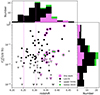Fig. 1. Selection of our diverse sample of LyC leakers (pink) from the Izotov et al. (2022, green) and LzLCS+ (black; Izotov et al. 2016a,b, 2018a,b, 2021; Wang et al. 2019; Flury et al. 2022a) samples. The x- and y- axis show the redshift and LyC escape fraction derived in the literature from fitting the COS UV spectrum, respectively (see Sect. 2.1). The triangle symbols show the $f_{\mathrm{esc}}^{\mathrm{LyC}}$ upper limits for the different samples. The dashed and dotted lines indicate the redshift corresponding to the wavelength cutoff of KCWI (λ = 3500 Å) and LRS2 (λ = 3650 Å), respectively. We show the redshift and $f_{\mathrm{esc}}^{\mathrm{LyC}}$ distributions at the top and right of the figure, respectively.

2.2. Observations and data reduction

Both IFU HET/LRS2 and Keck/KCWI data have been used to characterize the spatial distribution of our 22 galaxies (Sect. 2.1). Ten galaxies were observed with the blue configuration of LRS2 (refereed to as LRS2-B), and 12 with KCWI (see Table A.1 for details).

2.2.1. HET/LRS2

Our LRS2 (Chonis et al. 2016) observations were taken as part of the UT21-1-019, UT22-1-011, UT22-2-016 (PI: Chisholm), UT22-2-021 (PI: Leclercq), and UT22-3-011 (PI: Endsley) programs between January 2021 and December 2022 (see Table A.1). LRS2 is installed on the 10 m Hobby-Eberly Telescope (Ramsey et al. 1998; Hill et al. 2021) at the McDonald Observatory. LRS2 comprises two spectrographs separated by 100″ on sky: LRS2-B (with wavelength coverage of 3650 Å–6950 Å) and LRS2-R (with wavelength coverage of 6450 Å–10 500 Å). There are two channels for each spectrograph: UV and orange for LRS2-B and red and far red for LRS2-R. Each spectrograph has 280 fibers, each with a diameter of 0.59″, covering 6″ × 12″ with nearly unity fill factor (Chonis et al. 2016). The LRS2 spectral sampling is 0.7 Å per pixel and the spectral resolution varies from R ≈ 1500 to 2000, depending on the LRS2 spectrograph arm (UV: 1.63 Å, Orange: 4.44 Å, Red: 3.03 Å, Far red: 3.78 Å). We obtained LRS2-B observations for ten sources with total exposure time varying between 3600 and 17 400 s (see Table A.1). We also obtained LRS2-R observations that were combined to the LRS2-B datacubes during data reduction (see below), but did not use the LRS2-R data in this study.

We performed the LRS2 initial reductions using the Panacea¹ pipeline including: fiber extraction, wavelength calibration, astrometry, and flux calibration. On each exposure, we combined fiber spectra from the two channels into a single data cube accounting for differential atmospheric refraction (DAR). The DAR is taken into account by correcting the spatial shift channel by channel, using an empirical model for each channel built on tens of standard stars. We then identified the target galaxy in each observation by collapsing the cubes and by fitting the resulting white light images with a 2D Gaussian model. We finally rectified the data cubes to a common sky coordinate grid with the target at the center. To normalize each cube, we measured Hβ in both the LRS2-B and LRS2-R IFUs at the observed wavelength of ≈6564 Å at z ∼ 0.35. After normalization of blue and red cubes, we stacked the individual exposures together using a variance weighted mean. Our LRS2 data cubes have a spatial scale of $0\stackrel{″}{.}4$ by $0\stackrel{″}{.}4$ spatial pixels (spaxels) and are seeing-limited, with a median resolution of $\approx 1\stackrel{″}{.}74$ (∼9 kpc at z = 0.35). The LRS2 point spread function (PSF) of our observations was characterized by fitting standard stars observations using a Moffat function (Moffat 1969) to account for the PSF wings (see Appendix B.1). Throughout the paper, the LRS2 PSF is illustrated on figures with a blue circle whose size corresponds to the PSF full width at half maximum (FWHM).

For sky subtraction, we took the biweight spectrum of all spaxels at radius larger than 4″ from the target to minimize self-subtraction. Our galaxies are compact in SDSS (Flury et al. 2022a), ensuring that all the flux is included in the 4″ aperture. In addition, this 4″ aperture is larger than the curve of growth radius of the white light, Mg II and [O II] narrow band (NB) images for all the objects. The curve of growth radius (R_CoG) is defined as the radius at which the averaged flux in a 1-pixel wide annulus reaches zero (see Leclercq et al. 2017). Given that the sky varies from fiber to fiber over the 6″ × 12″ field of view of LRS2 (Chonis et al. 2016), we performed an additional residual sky subtraction. We modeled the sky residuals by masking in 2″ regions around the center of the galaxy as well as the emission lines of the galaxy (from Mg II to Hα) and by smoothing the data with a $2\stackrel{″}{.}5$ Gaussian kernel. This masked and smoothed sky residuals model is then subtracted from the data to obtain the final data cube.

2.2.2. Keck/KCWI

The KCWI observations were taken between 2019 and 2022 (PIs: Chisholm and Prochaska). The KCWI IFU offers several configurations with different gratings impacting the spectral resolution and wavelength range, and beam-slicers impacting the spatial resolution and field of view. For most of our observations, we choose a configuration consisting of the small image slicer and the BL grating with central wavelength of 4600 Å and a $8\stackrel{″}{.}4\times 20\stackrel{″}{.}4$ field of view with a 1 × 1 pixel binning. This combination allowed us to obtain a wavelength coverage of 3330−5937 Å (2467−4398 Å rest frame at z ∼ 0.35), a spectral resolution of R = 3600 (83 km s⁻¹) and a spatial sampling of $0\stackrel{″}{.}35\times 0\stackrel{″}{.}147$. We note that two objects have been observed with different configurations. J1503+3644 has a better spectral resolution than the rest of the sample (R = 8000 or 37 km s⁻¹) resulting in a shorter wavelength coverage (2700−3300 Å rest frame) that does not cover the [O II] 3727 Å doublet. J1014+5501 was observed with the medium slicer because of suboptimal transparency and thus has a spectral resolution of R = 1800 (166 km s⁻¹). We refer to Table A.1 for the configuration details of each target.

We used the KCWI KDERP pipeline Version 1.2.1² (Morrissey et al. 2018) to reduce our KCWI observations. Details about our KCWI KDERP data reduction steps and the CWITools pipeline can be found in King et al. (in prep.). Briefly, the major steps are the following: (1) bias and overscan subtraction, gain correction, cosmic rays removal; (2) dark and scattered light subtraction; (3) geometric transformation and wavelength calibration; (4) illumination correction and flat fielding; (5) standard sky subtraction; (6) data and variance cubes are produced in air wavelengths using the maps from (3); (7) differential atmospheric refraction correction using the observed airmass, the orientation of the image slicer, and the wavelengths of the exposures; (8) flux calibration using an inverse sensitivity curve made from standard star observations. After performing these eight steps, the final cubes were run through the CWITools pipeline (O’Sullivan & Chen 2020) in order to coadd the individual exposures and propagate the errors accordingly. The contributions from the individual input cubes were weighted by exposure time and projected on a common coadd grid with $0\stackrel{″}{.}14\times 0\stackrel{″}{.}14$ pixel size to optimize the spatial sampling (see Fig. 6 of O’Sullivan & Chen 2020), except for the J1014+5501 exposures which was observed with the medium slicer and projected on a common pixel grid of $0\stackrel{″}{.}29\times 0\stackrel{″}{.}29$. Every exposure was inspected and any exposure with poor seeing or cirrus absorption were discarded, leading to the total exposure time reported in Table A.1 with a minimum of 50 min on target.

The KCWI point spread function of our observations was characterized by modeling standards star observations using a Moffat function to account for the PSF wings (see Appendix B.1 for details). The median spatial resolution of the KCWI sample is 1″ or ∼5 kpc at the median redshift of the sample (Table B.1). Throughout the paper, the KCWI PSF is shown on figures with a blue ellipse whose size corresponds to the PSF FWHMs and position to the PSF rotation angle.

3. Mg II and [O II] spatial distributions

We now use the IFU observations of our sample of LyC leakers and non-leakers to characterize and compare the spatial extent of the neutral and low-ionization gas, using the Mg II 2796, 2803 Å line doublet (which traces species with ionization potential between 7.6 and 15 eV), and the ionized gas, using the [O II] 3727, 3729 Å line doublet (which traces species with ionization potential between 13.6 and 35.1 eV). We note that none of our galaxies show Mg I 2852 Å absorption (ionization potential of 7.6 eV), indicating that we do not detect gas in lower ionization state than Mg II. Consequently, Mg⁺ remains the sole ionization state coinciding with H⁰ in our observations, serving as our tracer for neutral and low-ionization gas.

We start by extracting Mg II and [O II] flux optimized NB images from the datacubes, as well as continuum images in Sects. 3.1 and 3.2, respectively. We then perform a 2D modeling procedure (Sect. 3.3) to characterize and compare the spatial extents (Sect. 3.4) and offsets (Sect. 3.5) of the different gas phases.

3.1. Narrow band image construction

We constructed Mg II and [O II] narrow band images of 12″ × 12″ and 8″ × 8″ from the LRS2 and KCWI datacubes, respectively. The LRS2 NB images are larger than the KCWI ones because they have a lower spatial resolution (see Table B.1); a larger spatial aperture is thus needed to encompass all the flux. These large spatial apertures ensure that all the detectable flux is included and that enough background is available to estimate the limiting surface brightness level (see below).

For each source, we constructed a continuum-only cube by performing a spectral median filtering on the data cube using a wide spectral window of 200 spectral pixels (see Herenz & Wisotzki 2017 for the validation of this continuum subtraction method on data cubes). After subtracting this continuum-only cube from the original one, we obtained an emission line only cube from which we optimally created the emission line NB images as follows: (i) we determine the spatial aperture that maximizes the integrated line flux by increasing the aperture until the integrated flux decreases because of the addition of noise, (ii) the line is extracted in the optimal aperture set in the previous step and its borders are determined by wavelengths for which the continuum subtracted flux density reaches zero, (iii) the NB image is created by summing the continuum-subtracted cube over the wavelength range delimiting the line. This procedure is applied to both the 2796 Å and 2803 Å lines of the Mg II doublet. The Mg II doublet lines are resolved and deblended at the resolution of our data in both LRS2 and KCWI datasets. The total NB image of the Mg II emission is finally obtained by adding the 2796 Å and 2803 Å NB images. We extracted the [O II] NB images from the data cubes using the same procedure. Given the resolution of our data, the [O II] line doublet is not fully resolved and is blended with the high-order Balmer lines H₁₃ 3722 Å and H₁₄ 3734 Å, so their borders are set when the flux increases again or manually when needed. We note that these Balmer lines are much fainter than [O II], so any contamination does not impact our results. We also note that with this procedure we miss the wings of the broader [O II] component, which represent a small percentage of the total flux. The resulting spectral windows used to create the Mg II 2796 Å, Mg II 2803 Å, and [O II] NB images are on average 5.5 Å, 5.0 Å and 11 Å wide in the observed frame, corresponding to 436 km s⁻¹, 396 km s⁻¹, and 655 km s⁻¹ at z ≈ 0.35 in the rest frame, respectively. The resulting Mg II and [O II] NB images, as well as their corresponding spectral windows, are shown in the middle panels of Figs. 2 and 3 for one strong LyC emitter (J1243+4646, $f_{\mathrm{esc}}^{\mathrm{LyC}}=89\%$) observed with KCWI and one weaker leaker (J1517+3705, $f_{\mathrm{esc}}^{\mathrm{LyC}}=4\%$) observed with LRS2, respectively. We note that the spectra shown in these figures were extracted in a different aperture (COS-like aperture of $2\stackrel{″}{.}5$) than the line used to determine the spectral width of the NB images (aperture maximizing the integrated flux). This aperture size (diameter) ranges from 3 to 8″ depending on the objects, and is on average two times larger (i.e., 5″) than the COS aperture. The figures for the whole sample can be found in the Appendix C.

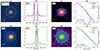Fig. 2. Example of a LyC leaking source (J1243+4646, $f_{\mathrm{esc}}^{\mathrm{LyC}}=0.889$) from our sample observed with KCWI. (a) 5″ × 5″ HST/COS acquisition image (when available) plotted with a power-law stretch. The circle indicates the 2$\stackrel{″}{.}$5 COS spectroscopic aperture (diameter). This aperture is also shown on the white light image e and was used to integrate the spectrum shown in panels b and f for comparison. (b) Observed Mg II line doublet extracted in a 2$\stackrel{″}{.}$5 aperture (units of erg s−1 cm−2 Å−1). The purple areas show the narrow band (NB) image spectral coverage. The vertical lines indicate the systemic redshift from Flury et al. (2022a) and Izotov et al. (2022). (c) 5″ × 5″ Mg II NB image plotted with a power-law stretch. The white contours correspond to Mg II significance levels of 3, 6 and 9σ (solid, dashed, and dotted, respectively). The blue circle shows the PSF FWHM estimated at Mg II wavelengths. The “+” and “x” symbols show the best-fit centroids of the emission line and nearby continuum, respectively. If neighboring sources were masked for the analysis, the mask is shown with an orange contour. (d) Radial surface brightness (SB) profiles of the observed and modeled Mg II emission (purple dots and line, resp.) compared to the modeled continuum (black) and PSF (blue) estimated at Mg II wavelengths. If the source is unresolved, the blue and black lines are under the purple or green line. The 3σ SB limit is shown as a dotted line. The shaded area represents the 1σ uncertainties from bootstrapping analysis. The horizontal error bars corresponds to the annulus width used to build the profiles. (e) IFU white light image. (f) [O II] line doublet (units of erg s−1 cm−2 Å−1). (g) Same as (c) for [O II]. (h) Same as (d) for [O II].

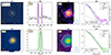Fig. 3. Same as Fig. 2 but showing one object (J1517+3705, $f_{\mathrm{esc}}^{\mathrm{LyC}}=0.04$) observed with LRS2. The size of the images is 10″ × 10″. The white areas are regions on the sky uncovered by our detector.

To determine the 1σ limiting flux value of the LRS2 NB images, we took the standard deviation of the pixels located outside a radius of 4″. This radius is larger than the curve of growth radius of the Mg II and [O II] emission line NB images, ensuring that we only select pixels with noise. The background pixels (r > 4″) were clipped (3σ) to eliminate the very noisy pixels (e.g., at the edges of the cubes). The LRS2 significance maps were then obtained by dividing the NB images by the corresponding 1σ flux limit value.

For the KCWI NB images, we used the variance from the data cubes to estimate the 1σ limiting flux. We checked that the errors from the KCWI error cubes were consistent with the values measured on the data using the same method as for the LRS2 data. We chose to use the values from the error cubes because they contain the pixel-per-pixel error information and therefore limit the impact of very noisy pixels. We note that the LRS2 pixel-per-pixel error information is not provided by the LRS2 data reduction pipeline. The KCWI significance maps were obtained by dividing the NB images by the square root of the corresponding variance images.

The contours in Figs. 2 and 3 show the 3, 6 and 9σ significance levels for the KCWI and LRS2 data. The resulting 1σ Mg II and [O II] limiting surface brightness (SB) values reach on average 8 × 10⁻¹⁸ and 3 × 10⁻¹⁸ erg s⁻¹ cm⁻² arcsec⁻², respectively. This is comparable to the previous KCWI studies (e.g., Burchett et al. 2021).

3.2. Continuum image construction

To compare the extent of the Mg II and [O II] emission to the stellar and nebular continuum and determine whether the metal line emission is more spatially extended than the continuum emission, we also generated continuum images from the data cubes. For Mg II, we averaged over two spectral windows located at ±1200 km s⁻¹ around the line doublet extremities, and that have the same velocity width as the corresponding NB image (on average 800 km s⁻¹ at z = 0.35 corresponding to the median redshift of the sample). These windows are close enough to the lines of interest and avoid the Mg I 2852 Å absorption line. For [O II], we averaged over one spectral window located at −2000 km s⁻¹ of the [O II] line doublet, and that has the same velocity width as the NB image (≈655 km s⁻¹). We refrain from using a window redder than the [O II] lines because of the numerous emission lines detected in this area. We have checked that using continuum windows at different velocities and total velocity widths do not affect the results.

We note that we did not attempt to disentangle the stellar and nebular continuum emission. The nebular continuum can contribute up to 20% to the observed continuum in highly ionized compact galaxies (Amorín et al. 2012). Given that the nebular continuum is generated from the gas surrounding the stars, it is expected to be more extended than the stellar continuum. Including the nebular continuum could thus lead to an overestimation of the size of the stellar continuum. However, this fact actually reinforces our conclusions (see Sect. 3.4).

3.3. Two-dimensional exponential modeling

To characterize the spatial distribution of our sources, we fit the NB images with a two-dimensional exponential distribution following previous studies of extended resonant emission lines (e.g., Lyα, Steidel et al. 2011). We used the python module LMFIT (Newville et al. 2014) and the following equation:

$$\begin{array}{c}\hfill C(r)=[I_{\mathrm{c}}exp(-r/rs)]\otimes {\mathrm{PSF}}_{2\mathrm{D},\mathrm{instr}}({\lambda }_{\mathrm{line}}),\end{array}$$(1)

with I_c and rs the central intensity and exponential scale length, respectively, and $r=\sqrt{{(y-y_0)}^2+{(x-x_0)}^2}$ with [x₀, y₀] the center coordinates. All parameters (center, scale length, and amplitude) are free to vary. The fit takes into account the PSF by convolving the model with the PSF kernel of the instrument (PSF_instr), which depends on the wavelength of interest (λ_line, see Appendix B). This approach holds the advantage to allow the direct comparison of the resulting parameters across different datasets acquired under varying conditions and utilizing different instruments. This particularly applies to our analysis, which involves separate datasets from two distinct instruments (Sect. 2). The neighboring galaxies visible in the NB images were masked to avoid contamination (J0130−0014 and J1256+4509).

We estimated the uncertainties associated with the best-fit parameters using a bootstrap Monte Carlo technique. We generated 100 instances of both the Mg II and [O II] NB images where each spaxel was randomly drawn from a normal distribution centered on the initial spaxel value and with standard deviation derived from the estimated median noise value for LRS2 data and from the variance image for the KCWI data (Sect. 3.1). Each realization of a given NB image set was fit as described above. The final best-fit values and associated errors were determined from the median and standard deviation, respectively, of the resulting parameter distributions.

The accuracy of size measurements for compact objects is impacted by the resolution limit due to the PSF. To establish the threshold scale length below which our measurements become unreliable, we ran our modeling procedure for a range of simulated flux distributions. These were generated using an exponential model combined with a random noise realization that matches our data, and convolved with the appropriate PSF based on the observed wavelength. For every modeled source, our fitting procedure was repeated 100 times using different noise realizations to determine the error on the retrieved scale length. We incrementally decreased the exponential scale length of the modeled source until we could no longer recover the input value. The scale length limit is a function of wavelength due to the PSF dependence on wavelength and thus on redshift. Consequently, we computed the resolution limit separately for each object in our sample, both for the Mg II and [O II] positions, and for each NB and continuum images. The resulting scale length resolution limits range from 0.6 to 1.6 kpc for the LRS2 data and, 0.3 to 1.2 kpc for the KCWI data. If the best-fit scale length fell below this resolution threshold, we considered the value as an upper limit. The spatial measurements and fitting results can be found in Table 2.

The fourth column of Figs. 2 and 3 (panels d) shows the data and best-fit model radial SB profiles obtained for the Mg II and [O II] emission as well as their respective continuum (see Appendix C for all objects). These profiles were computed by azimuthally averaging the flux over the continuum-subtracted NB and continuum images (Sects. 3.1 and 3.2) in concentric 2-pixel wide annuli (or $0\stackrel{″}{.}8$ and $0\stackrel{″}{.}3$ for LRS2 and KCWI data, respectively) centered on the Mg II best-fit centroids.

For most of the objects, the modeled radial SB profiles are a good representation of the observed profiles. We note that object J0130−0014 shows a SB excess at outer radii because of a close neighbor (Fig. C.1). In this case, our one-component model only describes the central object.

3.4. Spatial extent of the Mg II and [O II] emission

Of the 22 galaxies, two objects do not show any Mg II radiation (J0130−0014 and J0804+4726) and one (J1503+3644) lacks [O II] observations (Sect. 2.2.2). From our analysis of the PSF and detection limits (Appendix B and Sect. 3.3), we have identified four objects (J0130−0014, J0804+4726, J1154+2443, and J1256+4509) that have all of their measured scale lengths below their respective detection threshold. These objects are considered as unresolved in our study. Fourteen objects are resolved in Mg II, 13 in [O II] and 12 are resolved both in Mg II and [O II]. The average PSF-corrected Mg II and [O II] scale lengths (without accounting for upper limits) are 1.6 kpc and 1.4 kpc, respectively.

In order to evaluate whether the resolved emission lines are more spatially extended than the continuum, also referred to as “an emission line halo”, we calculated the probability p₀ of the two scale lengths to be identical by running a t-test for the objects without upper limits on their emission and continuum sizes. In case of an upper limit on the continuum scale length, we calculated the probability that the emission scale length is less than or equal to the continuum upper limit by considering a normal distribution. Out of the 14 objects with reliable Mg II scale length measurement, seven have a significant Mg II halo with p₀ < 10⁻⁵ (see Table 2 and left panel of Fig. 4). Among the 13 sources with robust [O II] scale length, ten have their [O II] emission more extended than the continuum with p₀ < 10⁻⁵ (see Table 2 and Fig. 4 middle panel). The Mg II and [O II] extended emissions have median extents being at least ∼1.4 and ∼1.5 times greater than the continuum, respectively. Interestingly, most of the objects with extended Mg II emission also show extended [O II] emission (except J1014+5501; we cannot conclude for J1503+3644 as [O II] observations are not available). Out of this sample of five galaxies that display both Mg II and [O II] extended emission, the Mg II emission is always more extended than [O II] (p₀ < 10⁻⁵) by a median factor of 1.2 (right panel of Fig. 4). The sole exception is potentially observed for J0844+5312, where the likelihood that the Mg II emission extends further than the [O II] emission is lower, but still possible with p₀ = 0.1. Conversely, five objects with extended [O II] emission are not extended in Mg II, suggesting that showing extended [O II] emission does not necessarily imply extended Mg II emission.

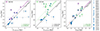Fig. 4. Comparisons of the spatial scale lengths (rs) as measured in Sect. 3.3: Mg II and continuum (left), [O II] and continuum (middle), and Mg II and [O II] (right). Objects with statistically significant Mg II and [O II] extended emission compared to continuum are indicated by large purple and green symbols, respectively (Sect. 3.4). Gray symbols in the right panel result in the overlap of the purple and green symbols and thus indicate that both Mg II and [O II] halos are detected. The dotted lines show by how much on average the emission is statistically more extended compared to the continuum (or emission) scale lengths: median ∼1.4 times for Mg II and ∼1.5 times for [O II] compared to the continuum, and 1.2 for the Mg II/[O II] ratio. The black line shows the 1:1 relation (i.e., no extended emission). Upper/lower limit values are shown with arrows. The Kendall correlation coefficient (τ) for every pair of variables and the corresponding false-positive probability that the correlation is real (p) are given and colored in green if the correlation is > 2σ statistically significant (Akritas & Siebert 1996; Flury et al. 2022b, see Sect. 3.4).

In order to quantify potential correlations with Mg II and [O II] spatial distributions, we computed the Kendall correlation coefficient (τ) following the Akritas & Siebert (1996) prescription for censored data to take into account the upper limits on variables. We used the routine described in Flury et al. (2022b)³ that also provides uncertainties on τ estimated by bootstrapping. Following Amorín et al. (2024) with a similar sample size, we considered correlations to be (i) significant if the false-positive probability (p) that the correlation is real is ≲2.275 × 10⁻² (2σ confidence) and (ii) strong if |τ|≳0.261. The Kendall correlation coefficients and corresponding false-positive probabilities of the tested correlations are reported in Table 3. While there is a 2σ correlation between the extent of the Mg II emission and continuum, we found that the spatial extent of the [O II] halo does not strongly depend on the stellar continuum size. The strongest correlation (> 3σ) is observed between the Mg II and [O II] scale lengths (Fig. 4). We also compared our Mg II scale length measurements with the UV half light radius ($r_{50}^{\mathrm{UV}}$, y-axis) measured in HST/COS data (Flury et al. 2022a; Izotov et al. 2022) and found a tentative < 2σ correlation (see bottom left panel of Fig. 9), suggesting a possible connection between the UV size of the galaxies and their Mg II spatial extent.

3.5. Spatial offset between Mg II, [O II], and the continuum

Our modeling procedure also provides us with centroid measurements for the emission line maps and their respective continua (Δ_{[Mg II]−cont} and Δ_{[O II]−cont} for Mg II and [O II], respectively). Our emission line to continuum spatial offset measurements range from no significant (< 3σ) offset to 2.83 kpc (J0919+4906) for Mg II and 2.16 kpc (J0804+4726) for [O II]. Seven objects have a > 3σ significant Mg II offset to the continuum. Most of our sources show a significant (> 3σ) spatial offsets between the [O II] emission and the continuum. Finally, 14 objects have a significant offset between Mg II and [O II] (see Table 2). The average Δ_{[Mg II]−cont}, Δ_{[O II]−cont} and Δ_{Mg II−[O II]} values (considering significant spatial offsets only) are 1.2, 0.5 and 0.9 kpc, respectively.

We find a tentative (2σ) correlation between the Mg II scale length and Δ_{[Mg II]−cont} (see top left panel of Fig. D.1 and Table 3). We do not observe such a correlation between the [O II] size and offset from the continuum (top right panel). We also report no correlation between the different scale length ratios (rs_Mg II/rs_cont, rs_[O II]/rs_cont, and rs_Mg II/rs_[O II]) and their respective spatial offsets (Δ_{[Mg II]−cont}, Δ_{[O II]−cont} and Δ_{Mg II−[O II]}). The corresponding figures can be found in the bottom panels of Fig. D.1.

We find that the Δ_{[Mg II]−cont} offset correlates with most of the galaxy size measurements (Mg II, [O II], and marginally with the continuum scale lengths, see Fig. D.2), including the half light radius as measured in Flury et al. (2022a) and Izotov et al. (2022) (right panel). This last correlation is weaker but holds, suggesting a tentative relationship between the size of the galaxies and their Mg II spatial offsets (see Table 3).

4. Connecting LyC leakage to gas distribution

Our characterization of the spatial distributions of the neutral and/or low-ionization and ionized gas in our galaxy sample unveils diverse gaseous configurations. Our targets indeed show from very compact (unresolved) to extended Mg II and [O II] emission (up to ∼10 kpc), as well as from significant (up to few kpc) to zero spatial offsets between the nebular gas and the stellar continuum. We now explore the connection between the spatial properties of the emitting gas and the escape of ionizing photons, derived in the literature from fitting the COS UV spectrum (Flury et al. 2022a; Saldana-Lopez et al. 2022; Izotov et al. 2022), using both individual (Sects. 4.1 and 4.2) and stacking measurements (Sect. 4.3).

4.1. Mg II and [O II] spatial extents versus $f_{\mathrm{esc}}^{\mathrm{LyC}}$

Figure 5 shows the connection between the escape of ionizing photons measured using the FUV continuum fits in Flury et al. (2022a) and the different exponential scale lengths from our analysis (Sect. 3.4). We found that most of the strong LyC leakers ($f_{\mathrm{esc}}^{\mathrm{LyC}}>5\%$) are unresolved, and therefore compact (rs ≲ 0.5 kpc), in both Mg II and [O II] emission (first and second panels), whereas the weaker or non leakers show a wider diversity with scale lengths ranging from upper limits (i.e., unresolved) to 3 kpc and 2 kpc for Mg II and [O II], respectively. We compute the fraction of strong LyC leakers (LCE detection fraction) detected in equal size bins of small and large scale lengths. Following Flury et al. (2022a), an object is considered as a strong leaker if $f_{\mathrm{esc}}^{\mathrm{LyC}}>5\%$ with > 5σ significance. The statistical uncertainties for fractions (i.e., Bernoulli trials) are given by a binomial proportion confidence interval using the Wilson approximation formula (Wilson 1927). Our 1σ uncertainties correspond to 68.3% confidence intervals. For Mg II, the LCE detection fraction in the rs_MgII < 1.3 kpc bin is 0.30${}_{-0.18}^{+0.45}$ and 0.10${}_{-0.04}^{+0.23}$ in the rs_MgII > 1.3 kpc bin. For [O II], the LCE detection fraction is 0.30${}_{-0.18}^{+0.46}$ in the rs_MgII < 1 kpc bin, and 0.18${}_{-0.09}^{+0.32}$ in the rs_MgII > 1 kpc bin. The trends with both scale lengths suggest that the LCE detection fraction decreases with increasing Mg II and [O II] spatial extents. We note that such a trend is more significant for Mg II.

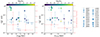Fig. 5. Relation between the LyC escape fraction and the spatial extent of the neutral and/or low-ionization (left panel) and ionized gas (right panel) as traced by the Mg II and [O II] scale lengths, respectively. The points are color-coded by the O32 values measured in Flury et al. (2022a). Objects with undetected Mg II are shown with higher transparency at x = 0. The red squares indicate the fraction of strong LyC leakers (5σ detection and $f_{\mathrm{esc}}^{\mathrm{LyC}}>5\%$ following Flury et al. 2022a) detected in the bin delimited by the horizontal error bars. The errors on the fractions correspond to a 1σ confidence interval (see Sect. 5.1). While weak and non LyC emitters show a wide diversity of Mg II and [O II] spatial extents, the neutral and/or low-ionization and ionized gas of strong leakers is compact (see Sects. 4.1 and 5.3).

Interestingly, J1033+6353 appears like an exception because it is a strong leaker ($f_{\mathrm{esc}}^{\mathrm{LyC}}\sim 30\%$) with large Mg II and [O II] spatial scale lengths (≈2 kpc). We also note that J0804+4726 is a strong leaker ($f_{\mathrm{esc}}^{\mathrm{LyC}}\sim 60\%$) with no Mg II detection and only an upper limit on its [O II] scale length. J0804+4726 has large uncertainties on its stellar continuum fit leading to a poorly constrained LyC escape fraction ($f_{\mathrm{esc}}^{\mathrm{LyC}}\simeq 0.58\pm 0.40$). This object is also our lowest metallicity source (12 + log₁₀(O/H) = 7.5), which might explain its weak Mg II emission. The LyC measurement for J1033+6353 is more reliable. We discuss this last object in Sect. 5.3.

When comparing the ratio between the emission and continuum scale lengths – excluding objects with upper limits on both their emission and continuum size measurements for which we cannot conclude (i.e., most of the strong leakers) – we do not find any strong correlation with $f_{\mathrm{esc}}^{\mathrm{LyC}}$ (Fig. E.1). Mg II and [O II] halos are indeed detected both in weak and non leakers. While J1033+6353 shows significant extended neutral and ionized gas, both Mg II and [O II] halos are less than 1.5 times more extended than the continuum. Objects with larger halos than J1033+6353 are all weak ($f_{\mathrm{esc}}^{\mathrm{LyC}}<3\%$) or non leakers. This is also valid when comparing the neutral and/or low-ionization and ionized gas extents; sources with Mg II more extended than [O II] are non-leakers (right panel). We note that our sample only includes 5 strong LyC leakers ($f_{\mathrm{esc}}^{\mathrm{LyC}}>5\%$) and that therefore larger samples are required to confirm these trends.

4.2. Spatial offsets versus $f_{\mathrm{esc}}^{\mathrm{LyC}}$

We now connect the LyC leakage fraction to the spatial offsets measured between the emission line and continuum centroids (Sect. 3.5). The first panel of Fig. 6 shows that strong leakers have zero or small (< 1 kpc) spatial offset between Mg II and the stellar continuum. We computed the LCE detection fraction similarly as in Sect. 4.1. We found that the LCE detection fraction significantly decreases with increasing Δ_{[Mg II]−cont}: 0.4${}_{-0.3}^{+0.6}$ in the Δ_{[Mg II]−cont} < 0.8 kpc bin and 0.0${}_{-0.0}^{+0.1}$ in the Δ_{[Mg II]−cont} > 0.8 kpc bin. We found a similar trend between $f_{\mathrm{esc}}^{\mathrm{LyC}}$ and the spatial offset between Mg II and [O II] centroids (right panel): the LCE detection fraction is 0.4${}_{-0.3}^{+0.6}$ in the Δ_{Mg II−[O II]} < 0.6 kpc bin, and 0.0${}_{-0.0}^{+0.1}$ in the Δ_{Mg II−[O II]} > 0.6 kpc bin. However, this trend is less significant when considering the spatial offset between [O II] and the continuum (middle panel): LCE detection fraction of 0.3${}_{-0.2}^{+0.4}$ in the Δ_{[O II]−cont} < 0.3 kpc bin, and 0.2${}_{-0.1}^{+0.4}$ in the Δ_{[O II]−cont} > 0.3 kpc bin. The same results are obtained when we normalize the offsets by the $r_{50}^{\mathrm{UV}}$.

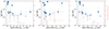Fig. 6. Relation between the LyC escape fraction and the spatial offset of the neutral and/or low-ionization (as traced by Mg II, Δ[Mg II]−cont, left panel) and ionized gas (as traced by [O II], Δ[O II]−cont, middle panel) from the stellar continuum. The right panel shows $f_{\mathrm{esc}}^{\mathrm{LyC}}$ as a function of the Mg II spatial offset relative to the [O II] centroid (ΔMg II−[O II]). The red squares indicate the fraction of strong LyC leakers detected in the bin shown by the horizontal error bars. The errors on the fractions correspond to a 1σ confidence interval (see Sect. 4.1). Symbols legend is the same as Fig. 5. While weak and non LyC emitters show a wide diversity of Mg II and [O II] spatial offset from the continuum, leakers have no/weak offset due to their compact configurations (see Sect. 4.1).

4.3. Mg II, [O II] and, continuum stacks

To increase the signal-to-noise ratio and determine the average SB profile of LyC leakers and weak or non leakers, we adopt a 2D stacking procedure. We only consider the objects with KCWI data because they were observed in very similar conditions (PSF FWHM ≈ 1″) compared to the LRS2 observations (see Table B.1). We exclude J0130−0014 because it has a larger PSF ($\mathit{FWHM}\approx 1\stackrel{″}{.}3$) and a bright neighboring source (see Fig. C.1). J1014+5501 is also excluded because it has a large PSF ($\mathit{FWHM}\approx 1\stackrel{″}{.}5$) and a different pixel scale because it was observed with a different slicer (see Table A.1). J0844+5312 has also been observed under less good conditions ($\mathit{FWHM}\approx 1\stackrel{″}{.}2$) but is included in the stacks. The inclusion of J0844+5312 does not change our conclusions. The KCWI targets used in the stack experiments have very similar redshifts (z = 0.34 − 0.43). We therefore do not rescale the flux of each individual image to correct for the impact of cosmological dimming. This affects individual galaxies at less than the 15% level (7% on average). We also do not normalize the flux of the images before stacking to retain physical units. However, we verify that the brightest sources are not dominating the composite images by ensuring that the normalization does not affect our results. We split our KCWI in two equal size subsamples resulting in five objects with $f_{\mathrm{esc}}^{\mathrm{LyC}}>4\%$ and five objects with $f_{\mathrm{esc}}^{\mathrm{LyC}}<4\%$. The continuum subtracted Mg II and [O II] images, and the continuum images were extracted as detailed in Sects. 3.1 and 3.2 (spatially centered on the continuum peak). Each subsample image was averaged using both median and mean functions for comparison. Figure 7 shows the resulting averaged stacks.

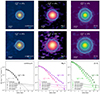Fig. 7. Composite images of our strong ($f_{\mathrm{esc}}^{\mathrm{LyC}}>4\%$, top row) and non and weak ($f_{\mathrm{esc}}^{\mathrm{LyC}}<4\%$, middle row) LyC leakers observed with KCWI (see Sect. 4.3). The UV continuum, Mg II and [O II] mean stacks are shown from left to right, respectively. The contours are spaced logarithmically by 0.2 dex, with the lowest contour level always at 4 × 10−18 erg s−1 cm−2 arcsec−2. The bottom row compares the continuum (left), Mg II (middle) and [O II] (right) radial SB profiles of the two subsets composites images. In each bottom panels, the lighter (darker) colored profiles with square (circle) symbols correspond to the strong (non/weak) LyC leaker subsample. The full and empty markers show the profiles of the median and mean composite images, respectively. The dotted lines correspond to the SB profiles of the median stacked PSF images of the different subsamples. The dashed lines show the 2σ significance levels.

Although our statistics are small, we gain a factor of more than 2.5 in terms of limiting SB levels compared to individual images, reaching levels of ≈1 × 10⁻¹⁸ and 3 × 10⁻¹⁸ erg s⁻¹ cm⁻² arcsec⁻² for the [O II] and Mg II composite images, respectively. We see a trend that both Mg II and [O II] are more extended than the continuum in weak/non LyC leakers ($f_{\mathrm{esc}}^{\mathrm{LyC}}<4\%$) compared to stronger leakers ($f_{\mathrm{esc}}^{\mathrm{LyC}}>4\%$). This is even clearer when comparing the radial SB profiles of the two subsamples (Fig. 7, bottom). While the emission lines are more extended, the continuum sizes are not significantly different, indicating that strong and weak LyC emitters have different nebular gas configurations. In addition of highlighting the compact/extended nature of the strong/weak leakers, the profiles reveal that the Mg II emission around weak/non leakers is more extended than the [O II] emission (Fig. 8 and Sect. 5.1). These stacking results are in good agreement with the trends from our individual analysis (Sects. 4.1 and 4.2). We however remind the reader that the individual measurements reveal a large diversity of spatial properties in the weak/non leakers sample.

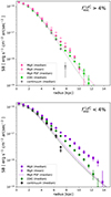Fig. 8. Direct comparison between the radial SB profiles of the strong ($f_{\mathrm{esc}}^{\mathrm{LyC}}>4\%$, top) and weak and non ($f_{\mathrm{esc}}^{\mathrm{LyC}}<4\%$, bottom) LyC leakers composite images. The legend is the same as in Fig. 7.

5. Discussion

Here we first contextualize our study within the broader CGM field by comparing our spatial measurements with previous results from the literature (Sect. 5.1). Then, we discuss the physical properties leading to compact nebular configurations (Sect. 5.2), the connection between spatial compactness and LyC escape fraction (Sect. 5.3), and finally, the impact of our results at high redshift (Sect. 5.4).

5.1. Previous results on extended Mg II and [O II] emission

Thanks to absorption studies (see Tumlinson et al. 2017, for a review), we know that galaxies are surrounded by metal-enriched gaseous halos. However, such pencil-beam surveys do not provide information about the morphology, porosity or global kinematics of the CGM. Detecting gaseous halos directly in emission would be ideal but is challenging because of their low surface brightness (≲10⁻¹⁸ erg s⁻¹ cm⁻² arcsec⁻²). Very recent work by Guo et al. (2023) reported the detection of Mg-enriched gas by stacking MUSE observations of z = 0.7 − 2.3 galaxies. This work revealed that the Mg II emission is statistically more extended than the stellar light and preferentially extends along the minor axis of massive galaxies (M_* > 10^9.5 M_⊙) following a biconical geometry tracing outflowing gas. Lower mass galaxies, resembling our galaxy sample, show rather circular Mg II distribution extending up to 10 kpc. Similarly, Dutta et al. (2023) stacked ≈600 galaxies of median mass M_* ∼ 2 × 10⁹ M_⊙ at z = 0.7 − 1.5 observed with MUSE and found Mg II emission extending up to 25 kpc at a SB level of 10⁻²⁰ erg s⁻¹ cm⁻² arcsec⁻². The ubiquity of Mg II halos is also observed in simulated star-forming galaxies, regardless of the stellar mass or redshift (Nelson et al. 2021). Although we expect Mg II halos to be universal, individual detections are still not very numerous in the literature. The few recent maps of extended Mg II emission around individual galaxies have been built due to sensitive IFUs such as MUSE or KCWI. Burchett et al. (2021) and Zabl et al. (2021) reported Mg II halos around two z ≃ 0.7 star forming galaxies, extending out from the galaxy center to a radius of ≈20 and 25 kpc at 1σ SB limits of 7 × 10⁻¹⁹ and 5 × 10⁻¹⁹ erg s⁻¹ cm⁻² arcsec⁻², respectively. Shaban et al. (2022) recently found patchy extended Mg II emission extending out to a radial distance of 27 kpc around a gravitationally lensed star-forming galaxy at z = 1.7 (1σ detection limit of ≈1 × 10⁻¹⁸ erg s⁻¹ cm⁻² arcsec⁻²). While these galaxies from the literature are at higher redshift and are more massive than our sample (z ∼ 0.35, M_* ∼ 10⁹ M_⊙), our 7 Mg II halos have similar maximal spatial extents (≈10 − 20 kpc at a 1σ SB limit of 8 × 10⁻¹⁸ erg s⁻¹ cm⁻² arcsec⁻²) and comparable Mg II to continuum extent ratios (visually determined from Zabl et al. 2019; Burchett et al. 2021; Shaban et al. 2022 to range from 1.2 to 2.5). This suggests that the Mg II spatial extent does not strongly depend on stellar masses or redshift, in agreement with the simulation work of Nelson et al. (2021). The observed spatial extent values are however more than ten times larger than the simulated spatial extents of Nelson et al. (2021) at a fixed SB of 1 × 10⁻¹⁸ erg s⁻¹ cm⁻² arcsec⁻² in the z ∼ 0.3 redshift bin and the smallest (M_* ∼ 10⁹ M_⊙) mass bin (their Fig. 3). Given that these simulations do not take into account radiative transfer effects, this difference suggests that Mg II resonant scattering has a strong effect on the Mg II halos spatial extents. Larger samples will be needed to understand which galaxy properties drive the size of the Mg II halos and their evolution.

Similarly to our results, most of the studies cited above also report [O II] emission more extended than the stellar continuum when Mg II is extended, both in stacks and individual objects. In particular, our stack experiment reveals for the first time that on average Mg II is statistically more extended than both the continuum and [O II] for objects with $f_{\mathrm{esc}}^{\mathrm{LyC}}<4\%$. This is expected when there are numerous resonant scatterings that propagate Mg II photons out spatially. In individual objects, Mg II also appears more extended than [O II] (see Zabl et al. 2021, and some objects of our study), but we also find a large diversity of configurations with sources showing similar Mg II and [O II] extents or larger [O II] scale lengths. Dutta et al. (2023) found [O II] to be more extended in their composite images of galaxies within large scale groups where environmental effects could be at play. Rupke et al. (2019) also discovered a [O II] nebula that extended 100 kpc around a massive galaxy (M_* ∼ 10¹¹ M_⊙) at z = 0.46 (1σ SB limit of 1 × 10⁻¹⁸ erg s⁻¹ cm⁻² arcsec⁻²), with Mg II emission a lot more compact than [O II]. We find similar objects in our sample, with five galaxies showing ionized [O II] gas but no extended neutral and/or low-ionization gas, as traced by Mg II. We also note that our ground-based data do not resolve some of the most extreme LyC leakers, leaving the full picture for their extent largely unclear. Overall, our Mg II and [O II] halo properties are comparable to previous studies reported in the literature.

Finally, while our metal-enriched emitting halos are ≈10 times less extended than their continuum compared to the high redshift Lyα halos (z > 3, e.g., Wisotzki et al. 2016, 2018; Leclercq et al. 2017; Kusakabe et al. 2020; Claeyssens et al. 2022), we find similar emission to continuum size ratios (rs_Mg II/rs_cont and rs_[O II]/rs_cont ranging from 1 to 3) as for the Lyα and Hα halos reported in nearby galaxies (Hayes et al. 2013; Rasekh et al. 2022). In contrast with the Mg II halos, Rasekh et al. (2022) report a correlation between the size of the Lyα halos and the stellar masses. Larger samples of Mg II halos will be needed to understand this difference.

5.2. Physical properties for compact Mg II and [O II] gas configurations

Here we investigate whether any physical parameters impact the neutral and ionized gas extent. We compare the Mg II exponential scale lengths measured on our statistical sample of 22 objects with their global properties as measured in Flury et al. (2022a), Izotov et al. (2022) and Saldana-Lopez et al. (2022) in Fig. 9. We find significant correlations with the O₃₂ ratio, Hβ equivalent width, metallicity, and marginally with $r_{50}^{\mathrm{UV}}$ and the H I covering fraction C_f(H I) (see Table 3). In other words, compact configurations of the neutral and/or low-ionization gas are preferentially found in galaxies with high ionization parameter, large Hβ equivalent width (EW), low metallicity, low H I covering fraction, and rather compact in UV sizes. The spatial extent of the ionized gas, as traced by [O II], is even more strongly correlated (> 3σ) with these exact same quantities. The fact that we observe weaker correlations for Mg II could be due to the fact that (i) Mg II is intrinsically fainter than [O II] and (ii) Mg II resonant scattering increases the chances for Mg II photons to be absorbed by dust, adding scatter in some correlations. We find no correlations with E(B − V), UV β¹⁵⁰⁰ slope, stellar mass, star formation rate (SFR), SFR surface density, specific SFR, or stellar age. We also report a lack of strong correlation between the Mg II spatial extent and the Lyα equivalent width or escape fraction. While the E(B − V), UV β¹⁵⁰⁰ slope, SFR surface densities, and Lyα escape fraction tend to correlate with $f_{\mathrm{esc}}^{\mathrm{LyC}}$ (e.g., Flury et al. 2022b; Begley et al. 2024), they do not significantly scale with the Mg II spatial extent. Most of these noncorrelations are also observed for the Lyα spatial extents. Rasekh et al. (2022) indeed found no correlation between the dust attenuation and the Lyα halo scale length of their low-z galaxies. Moreover, they only found a weak correlation with the Lyα EW (see also Leclercq et al. 2017 where no correlation is found for galaxies at z > 3), and no trend with the Lyα escape fraction. These results suggest that the relationship between the galaxy properties and their neutral and low ionization gas distribution is complex and underscore the need for larger samples and higher spatial resolution to better understand the physical processes that govern the spatial extent of the neutral gas around galaxies.

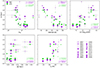Fig. 9. Comparisons of the emission scale lengths (Mg II in purple and [O II] in green) and the O32 ratios (top left), Hβ equivalent widths (top middle), metallicities (top right), UV half-light radii (bottom left), and H I covering fractions (bottom right). Upper limit values are shown with arrows. The Kendall correlation coefficient (τ) for every pair of variables and the corresponding false-positive probability that the correlation is real (p) are given for both emission lines in the top right corners following the same color coding as the data points (Akritas & Siebert 1996; Flury et al. 2022b, see Sect. 3.4).

The inverse correlation between the ionization of the galaxy and the total extent of the neutral and/or low-ionization gas suggests that galaxies that have more compact neutral gas sizes are more highly ionized. This could arise from the stellar populations within the galaxies ionizing most of the neutral gas within the galaxy and halo, such that galaxies with high O₃₂ and large Hβ equivalent widths ionize all of the neutral gas within 1 kpc. The literature has often called this a “density-bounded” ISM configuration (e.g., Jaskot & Oey 2013; Nakajima & Ouchi 2014; Gazagnes et al. 2018, 2020). In other words, such compact objects might have a ISM/CGM with very low H I column density. This is consistent with the low H I covering fraction (0.38 < C_f(H I) < 0.63) measured in Saldana-Lopez et al. (2022) for the objects with compact configurations (< 1 kpc, except for J1033+6353 discussed in Sect. 5.3). Conversely, the most extended objects (rs > 1 kpc) show higher values (0.63 < C_f(H I) < 0.99) indicating the presence of larger amount of neutral gas. The detection of double-peaked Lyα profile with narrow peak separation observed in strong LyC emitting galaxies (e.g., Verhamme et al. 2017; Izotov et al. 2018b, 2021) is also in good agreement with compact objects having low H I column densities. This is also consistent with the results of Kanekar et al. (2021) that report a low H I 21 cm detection rate in local compact galaxies with the high (> 10) O₃₂ ratios. We discuss the relationship between the compactness and the LyC escape in the next section (Sect. 5.3).

5.3. LyC escape and spatial compactness

Flury et al. (2022b) found a scattered but significant correlation between the UV half-light radius measured on the COS acquisition images and $f_{\mathrm{esc}}^{\mathrm{LyC}}$, indicating that strong LyC emitters have compact stellar cores. In this work, we looked at the nebular gas distribution and similarly found that strong leakers have very compact gas distributions. The LCE detection fraction is indeed higher at small Mg II and [O II] spatial extents (Sect. 4 and red points in Fig. 5). This is in agreement with the recent work of Choustikov et al. (2024) where they found that galaxies with high $f_{\mathrm{esc}}^{\mathrm{LyC}}$ tend to have less extended neutral gas (Lyα) halos than non-leaking sources. These results indicate that the CGM of strong leakers has a low H I column density, which would allow the LyC photons that escape the ISM to go through the CGM without being absorbed. These low column densities in the galaxy surroundings can be caused by stellar populations within galaxies ionizing most of the neutral gas in the CGM (see Sect. 5.2) and/or powerful outflows and feedback effects capable of clearing the galaxy surroundings (Chisholm et al. 2017; Trebitsch et al. 2017; Carr et al. 2021, but see Jaskot et al. 2017). Indeed, Amorín et al. (2024) recently found that the strongest LyC emitters show strong indication of ionized outflows and more complex kinematics. We note that we plan to analyze the resolved kinematics of our KCWI sources in future work (Leclercq et al., in prep.) Such effects might be even more important at high redshift with the increase in ionization of galaxies (e.g., Endsley et al. 2021; Rinaldi et al. 2023; Cameron et al. 2023), and the presence of higher velocity (Sugahara et al. 2019, z ∼ 5 − 6) and more frequent spherical outflows (Xu et al. 2023b, z ∼ 3 − 9). Moreover, in the nearby reionization-era analog galaxy Haro 11, Le Reste et al. (2024) showed that merger-driven interactions can induce a significant shift of neutral gas by several kpc from the galaxy center, facilitating LyC escape in our line of sight. The compactness of the nebular gas in strong LyC leakers, coupled with its link to highly ionized and density-bounded interstellar medium configurations (Sect. 5.2), may elucidate the mechanism behind the escape of ionizing photons from these galaxies.

The J1033+6353 galaxy however behaves differently compared to the other strong LyC emitters which might indicate a different leakage mechanism. It is indeed the only strong leaker of the sample with $f_{\mathrm{esc}}^{\mathrm{LyC}}$ ≈ 30% to show Mg II emission, i.e., neutral and/or low-ionization gas, beyond its stellar continuum. Although Mg II is only more extended than the continuum by a factor 1.5, this result suggests that the presence of neutral and/or low-ionization gas in the CGM is not incompatible with strong LyC leakage, which might thus escape anisotropically through ionized channels that go through both the ISM and CGM, as proposed in the literature (Borthakur et al. 2014; Trebitsch et al. 2017; Gazagnes et al. 2018, 2020; Wang et al. 2019; Mauerhofer et al. 2021; Flury et al. 2022b). This scenario is reinforced by the detection of extended [O II] emission that traces the ionized gas. Moreover, Saldana-Lopez et al. (2022) measured a relatively low H I covering fraction of C_f(H I) ≈ 0.6 for J1033+6353 compared to the rest of the sample (0.4 < C_f(H I) < 1) which favors a patchy configuration of the ISM/CGM. Interestingly, J1033+6353 has a lower O₃₂ ratio (≈5) compared to the other strong leakers (> 14). This suggests that LyC photons may escape J1033+6353 through ionized channels that cross through otherwise lower ionization gas (e.g., Flury et al. 2022b).

Finally, it is important to highlight that our study has revealed that weak and non LyC leakers show diverse Mg II and [O II] spatial extents spanning from compact to > 3 times more extended than the stellar continuum (Sect. 4.1). The compact nebular configurations of weak and non LyC leakers indicates that the LyC photons are absorbed within the ISM. Higher spatial resolution data is needed to get better understanding of the physical state of the ISM/CGM and the inner propagation of the LyC photons.

5.4. Using nebular gas extent to infer $f_{\mathrm{esc}}^{\mathrm{LyC}}$ at high redshift

Recent JWST observations reveal that galaxies are compact at z > 6 with effective radii ≲1 kpc (e.g., Naidu et al. 2022a; Yang et al. 2022; Ono et al. 2023; Robertson et al. 2023; Ormerod et al. 2024). Moreover, Mg II has been detected at very high redshift (e.g., GNz11 Bunker et al. 2023; Gazagnes et al., in prep.). Although only few spatial measurements of the nebular gas at such high redshift exist (e.g., Arribas et al. 2024), we discuss the possibility of using the Mg II and [O II] compactness as an indicator of leakage in the EoR. Our study has revealed that the neutral and ionized gas distributions of most LyC emitting galaxies have compact configurations. However, we also found that weak LyC emitters or non leakers are diverse, with some also showing compact configurations. As a consequence, a compactness criterion is not enough to disentangle the population of strong and weak leakers. Figure 5 shows the relation between the spatial extent of the gas and $f_{\mathrm{esc}}^{\mathrm{LyC}}$ with data points color coded by the O₃₂ ratios. Combined with other diagnostics such as strong O₃₂ ratio, high Hβ equivalent width, or low metallicity, Mg II and [O II] spatial compactness (although [O II] is slightly less statistically reliable) appear like good indicators of LyC escape. As an example, we can expect high redshift Mg II and [O II] emitters unresolved in NIRSpec/IFU (≲0.5 kpc at z = 7 considering the spatial scale of $0\stackrel{″}{.}1$) and with high O₃₂ ratios to be leaking ionizing photons.

6. Summary and conclusions

Thanks to our IFU campaigns targeting stringently confirmed LyC emitters and non-emitters with KCWI and LRS2, we characterized the gas distributions of 22 z ≈ 0.35 galaxies and connected their spatial properties to the escape of ionizing photons. We used Mg II as a tracer of neutral and low-ionization gas and [O II] as a tracer of ionized gas. The spatial distributions were parameterized individually using a 2D exponential model. In order to confirm the trends observed for individual objects between the neutral and/or low-ionization and ionized gas distribution properties and the escape of ionizing photons, we performed stacking experiments. Our results can be summarized as follows:

1. The radial surface brightness profiles of the Mg II, [O II], and continuum emission are reasonably well-fit by an single component exponential model (Sect. 3.3). The average Mg II and [O II] exponential scale lengths of our sample (without accounting for upper limits) are 1.6 kpc and 1.4 kpc, respectively. Out of the 14 (13) objects with reliable Mg II ([O II]) scale length measurement, seven (ten) have a significant Mg II ([O II]) halo extending up to > 10 kpc (Sect. 3.4).

2. The Mg II and [O II] extended emission have median extents being at least ∼1.4 and ∼1.5 times greater than the continuum respectively. Most of the objects with extended Mg II emission also show extended [O II] emission (all but one object); in this case, Mg II emission is always more extended than [O II] by a median factor of 1.2. Five objects with extended [O II] emission are not extended in Mg II, suggesting that extended [O II] emission does not necessarily imply Mg II extended emission (Sect. 3.4).

3. We observed a 2σ correlation between the Mg II emission and continuum extents and a > 3σ correlation between the Mg II and [O II] scale lengths (Sect. 3.4).

4. Our emission line to continuum spatial offset measurements range from no significant offset to 2.8 kpc and 2.2 kpc for Mg II and [O II], respectively. The average Δ_{[Mg II]−cont}, Δ_{[O II]−cont} and Δ_{Mg II−[O II]} values are 1.2, 0.5 and 0.9 kpc, respectively (Sect. 3.5).

5. We find that the Mg II offset correlates with the galaxy size measurements (Mg II, [O II], and continuum scale) and NUV half-light radius. We do not observe such a correlation for [O II]. We also report no correlation between the Mg II/continuum, [O II]/continuum and Mg II/[O II] scale length ratios and their spatial offsets (Sect. 3.5).

6. The strong LyC leakers ($f_{\mathrm{esc}}^{\mathrm{LyC}}$ > 5%) are unresolved, and therefore compact (rs ≲ 0.5 kpc), in both Mg II and [O II] emission, whereas the weaker or non leakers show a wider diversity with scale lengths ranging from upper limits (i.e., unresolved) to 3 kpc and 2 kpc for Mg II and [O II], respectively. The LCE detection fraction decreases with increasing Mg II and [O II] spatial extents (Sect. 4.1). The same results are obtained when we normalize the offsets by the $r_{50}^{\mathrm{UV}}$.

7. Strong leakers have zero or small (< 1 kpc) spatial offset between Mg II and stellar continuum. The LCE detection fraction significantly decreases with increasing Mg II-continuum offset. We found a similar trend between $f_{\mathrm{esc}}^{\mathrm{LyC}}$ and the spatial offset between Mg II and [O II] centroids (Sect. 4.2).

8. Stacking experiments of our KCWI reinforce the trends observed for individual objects that the Mg II and [O II] emission are more extended in non/weak LyC leakers than in strong leakers. Independently of $f_{\mathrm{esc}}^{\mathrm{LyC}}$, Mg II is found to be more extended than [O II] on average (Sect. 4.3).

9. Our Mg II and [O II] halos properties are comparable to previous studies. We found significant anticorrelations between the spatial extent of the neutral and/or low-ionization gas and the O₃₂ ratio, and Hβ equivalent width, as well as positive correlations with metallicity, and marginally, the H I covering fraction and UV size, suggesting that galaxies that have more compact neutral gas sizes are more highly ionized (Sect. 5.2). We find no correlations with E(B − V), UV β¹⁵⁰⁰ slope, stellar mass, SFR, SFR surface density, specific SFR, stellar age, EW(Lyα), and Lyα escape fraction.

10. The fact that the LCE detection fraction is higher at small Mg II scale lengths indicates that the CGM of strong leakers has a low H I column density caused by stellar populations ionizing most of the surrounding neutral gas (Sect. 5.3). J1033+6353 is a strong leaker with a lower O₃₂ ratio (≈5) than other strong leakers (> 14) surrounded by a Mg II halo, suggesting a different leakage mechanism where LyC photons escape through ionized channels that go through both the ISM and the CGM (Sect. 5.3).

11. Combined with high ionization diagnostics such as strong O₃₂ ratio, high Hβ equivalent width or low metallicity, Mg II and [O II] spatial compactness appear like good indicators of LyC escape in the EoR (Sect. 5.4).

Our IFU study of the spatial distribution of the neutral and ionized gas around a statistical and robust sample of 22 LyC emitting and non emitting galaxies has revealed a large diversity of gas configurations within the sample, with a trend for strong leakers to be compact. Our findings suggest that highly ionized galaxies are not surrounded by extended gaseous envelopes, implying that LyC photons can escape in many directions due to a widespread ionization and/or due to an ISM with numerous porous lines of sight distributed fairly isotropically. We therefore propose to use the compactness of the neutral and ionized gas around galaxies as an additional LyC leakage indicator. A future paper will delve into the kinematics and resolved properties maps derived from our IFU data, complementing the spatial insights presented in this paper (Leclercq et al., in prep.). Larger samples with deeper and higher resolution IFU observations will be needed to get a deeper understanding of the mechanisms governing ionizing photon escape in galaxies. The Lyα and Continuum Origins Survey (LaCOS) is a 119-orbit HST program (PID 17069) that will obtain spatially resolved images of 41 LzLCS+ galaxies. Simultaneously, we will obtain high resolution Lyα spectra for 15 LzLCS+ galaxies using HST/COS (PID 17153). The Lyα images and spectra will unveil the physical state of the ISM/CGM and its role in regulating LyC escape. Connecting the Lyα properties with the Mg II will help understand how Mg II can be used at the EoR (when Lyα is not observable) to constrain the LyC transmission in the JWST era.

Acknowledgments

We thank the referee for insightful and useful comments that significantly improved the clarity and scope of this paper. This research is based on observations made with the NASA/ESA Hubble Space Telescope obtained from the Space Telescope Science Institute, which is operated by the Association of Universities for Research in Astronomy, Inc., under NASA contract NAS 5–26555. These observations are associated with program 15845. The Low Resolution Spectrograph 2 (LRS2) was developed and funded by the University of Texas at Austin McDonald Observatory and Department of Astronomy and by Pennsylvania State University. We thank the Leibniz-Institut für Astrophysik Potsdam (AIP) and the Institut für Astrophysik Göttingen (IAG) for their contributions to the construction of the integral field units. We would like to acknowledge that the HET is built on Indigenous land. Moreover, we would like to acknowledge and pay our respects to the Carrizo & Comecrudo, Coahuiltecan, Caddo, Tonkawa, Comanche, Lipan Apache, Alabama-Coushatta, Kickapoo, Tigua Pueblo, and all the American Indian and Indigenous Peoples and communities who have been or have become a part of these lands and territories in Texas, here on Turtle Island. We acknowledge the Texas Advanced Computing Center (TACC) at The University of Texas at Austin for providing high performance computing, visualization, and storage resources that have contributed to the results reported within this paper. The authors wish to recognize and acknowledge the very significant cultural role and reverence that the summit of Maunakea has always had within the indigenous Hawaiian community. We are most fortunate to have the opportunity to conduct observations from this mountain. Y.I. acknowledges support from the National Academy of Sciences of Ukraine (Project No. 0121U109612). R.A. acknowledges support from ANID/Fondecyt 1202007. O.B. is supported by the AstroSignals Sinergia Project funded by the Swiss National Science Foundation. M.T. acknowledges support from the NWO grant 016.VIDI.189.162 (“ODIN”).

References

Appendix A: Table of the observations

Appendix B: Point spread function characterization

Here we provide a detailed description of our procedure to characterize the point spread function (PSF) for both our LRS2 (B.1) and KCWI (B.2) observations. The resulting PSF parameters can be found in Table B.1.

B.1. KCWI PSF

To characterize the PSF of the KCWI instrument, we fit standard stars that were observed immediately before or/and after the science observations. Given that one of our primary scientific objectives involves the detection of extended emissions, we devoted particular attention to understanding the wings of the PSF.

The comparison between the Gaussian and Moffat best-fit models, as illustrated in Fig. B.1 indeed reveals that a Gaussian PSF model does not capture the PSF wings. Consequently, utilizing a Gaussian model would artificially lead to the detection of extended emissions. We therefore adopted a Moffat PSF model and fit the standard star observations at the wavelengths pertinent to this study, i.e., Mg II (≈ 3790 Å) and [O II] (≈ 5045 Å) and within a window of ≈ 1000 km s⁻¹ (or 13 Å at z = 0.35). We note that some objects of our sample have two standard stars observations (before and after the science observations). In this case, we consider the average of the two sets of Moffat parameters set as PSF parameter values. The errors on the PSF model parameters were estimated using a bootstrapping Monte Carlo method. Given the brightness of the standard stars, the resulting errors on the PSF parameters are small. The average uncertainties are 0.001″, 0.05, and 0.001 degree for the FWHM, β and ϕ values, respectively. The resulting elliptical Moffat model parameters are compiled in Table B.1.

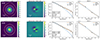Fig. B.1. Characterization of the KCWI point spread function. Example for the standard star (Feige66) where the first and second rows show the size measurement at Mg II (≈ 3790 Å) and [O II] (≈ 5045 Å) wavelengths of the corresponding science object observed (J1256+4509), respectively. First panel: Narrow-band image at the wavelengths of interest (≈ 1000 km s−1 wide or 13 Å at z = 0.35). The white and orange contours corresponds to SB levels of 10−14, 10−13, and 10−12 erg s−1 cm−2 arcsec−2 for the data and Moffat best-fit model, respectively. Second panel: Fit residuals of the Moffat best-fit model. Third panel: Radial SB profiles of the standard star data (black), Gaussian best-fit model (blue) and Moffat best-fit model (orange). The best-fit model parameters are shown in the bottom left. Forth panel: Zoom-in on the inner profiles. A Moffat model better describes both the core and wings of the PSF for our KCWI observations.

B.2. LRS2 PSF

We applied the same fitting process as for the KCWI standard stars (Sect. B.1). We selected standard stars observed on the same night as the science observations and fit them with an elliptical Moffat model. This fitting was performed within a ≈ 1000 km s⁻¹ spectral window around both the Mg II and [O II] wavelengths of the science object, which correspond approximately to 3780 Å and 5030 Å, respectively. Similarly to the KCWI standard stars observations, the core and wings of the LRS2 PSF are better described by a Moffat distribution than a Gaussian model (see Fig. B.2 for the example of BD+210607). Moreover, our measurements show that the LRS2 PSF is consistent with being circular with a mean axis ratio of 0.97 ± 0.08 (Fig. B.3, first panel). Characterizing the PSF of our LRS2 observations is however more challenging than for the KCWI observations. This is because standard stars are not always observed right after our main observations, but at the end of the night when the seeing conditions are not as good as during our main observations. As a result, our PSF size estimates would end up being larger than what it actually is, which would hamper a precise spatial analysis.

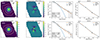Fig. B.2. Same as Fig. B.1 but for the LRS2 PSF characterization. We show the size measurements of the standard star BD+210607 observed at the end of the night of the J0804+4726 observations. We do not include a rotation measurement because most of the standards stars can be considered as circular (see Fig. B.3). The size of the stars as observed with LRS2 and therefore the LRS2 PSF is better described with a Moffat model.

In order to best characterize the PSF of our observations and its evolution with wavelength, we adopt the following approach. The only information that we have about the seeing conditions during the science observations is the DIMM seeing at the telescope which is reported in the observation log. We show in Fig. B.3 (second to fourth panels) that the DIMM seeing size reported during the standard stars observations provides a reasonably good estimation of the PSF FWHM near the central wavelength of LRS2 (≈ 5300 Å), but underestimates the PSF size at Mg II wavelengths (≈ 3780 Å). This discrepancy arises because the PSF shape evolves as a function of wavelength. We measured this evolution for each standard star observation by dividing the datacubes into 14 wavelength slices of 250 Å. The first and second panels of Figure B.4 shows the PSF FWHM as a function of wavelength for the standard star BD+210607 (blue) and all the standard stars observed on the same nights of our science observations, respectively. As expected, we observe a decrease in FWHM with increasing wavelengths. The median slope of this decrease is −9 ± 4 × 10⁻⁵ (third panel). The PSF size at the wavelength of interest can then be estimated using this slope and the DIMM seeing of the observations – under the assumption that the DIMM seeing is a good approximation of the PSF FWHM at 5300 Å which is the case for our data (see second panel of Fig. B.3) – using this equation:

$$\begin{array}{c}\hfill FWH{M}_{\mathrm{PSF},\mathrm{LRS}2}(\lambda )=-9\times {10}^{-5}(\lambda -5300\mathrm{\AA })+\mathrm{DIMMseeing},\end{array}$$(B.1)

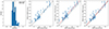Fig. B.3. LRS2 PSF shape and estimation of its FWHM based on the DIMM seeing. Left panel: Distribution of the FWHM PSF ratio, Q(FWHM) = FWHMX/FWHMY, measured on the standard stars observed with LRS2. The PSF is on average consistent with being circular with a mean FWHM ratio of 0.97±0.08. Second left to right: Comparison between the DIMM seeing at the telescope and the FWHM (mean between the x- and y-axis of the elliptical Moffat function, see Fig. B.2) measured on the standard stars (Sect. B.2) at the middle of the LRS2-B wavelength window (∼ 5300 Å), at the Mg II and at the [O II] wavelengths, respectively. The dashed line shows the one-to-one relation. The DIMM seeing provides a relatively good estimation of the PSF FWHM near ∼ 5300 Å but overestimates it at Mg II wavelengths (≈ 3780 Å). The red line shows the estimated PSF FWHM based on the DIMM seeing calculated using Eq. B.1 (see Sect. B.2).

where the wavelength λ is in units of Å and the FWHM and DIMMseeing in arcsec. This relation applied at the observed Mg II and [O II] wavelengths (≈3780 Å) is showed in red in the third and fourth panels of Fig. B.3. The estimated PSF based on the DIMM seeing (Eq. B.1) is now closer to the observed values. We performed the same exercise for the Moffat shape parameter β. The fourth panel of Fig. B.4 shows the individual standard star measurements along with the overall trend of β evolution with wavelength. We highlighted the measurements of BD+210607 as example (blue). While doing this analysis, we found that the individual FWHM(λ) slope and beta values measured for each standard star can be quite different from the average values across all the standard stars. We therefore decided to use the individual slope and β measurements, rather than the average values. These individual measurements are reported in Table B.1. As for KCWI, we note that some objects of our sample have several standard stars observations. In this case, we consider the average of the different sets of Moffat parameters set as PSF parameter values. The errors on the PSF model parameters were estimated using a bootstrapping Monte Carlo method. The average uncertainties are 0.02″ and 0.5 for the FWHM and β values, respectively.

Fig. B.4. First panel: Evolution of the PSF FWHM with wavelength for the standard star BD+210607 observed with LRS2. The vertical dashed line indicate the Mg II and [O II] wavelengths of the science object J080425+472607. The vertical dotted blue line corresponds to the central wavelength of LRS2B (≈ 5300 Å). The solid blue line shows the best first-order polynomial fit to the data. The resulting slope is −9 × 10−5 which is consistent with the average value obtained from all the standard stars (middle and right panels). Second panel: Best first-order polynomial fits of the PSF FWHM – wavelength relation of all the standard stars (gray). The relation resulting from the median slope and the standard deviation is shown with solid and dotted black line, respectively. Third panel: Distribution of the slope measured on the standard stars. The solid and dotted vertical lines indicate the median and standard deviation of the distribution (values on middle right), respectively. Fourth panel: Evolution of the Moffat β parameter with wavelength for all the standard stars (gray). The empty squares and corresponding errorbars give the median value and median absolute deviation in each wavelength bin. The blue dots show the BD+210607 values.

Appendix C: Mg II and [O II] maps and SB profiles

Fig. C.1. Same as Fig. 2 (Part 1/8).

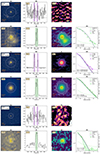Fig. C.1. Continued (2/8).

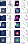Fig. C.1. Continued (3/8).

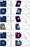Fig. C.1. Continued (4/8).

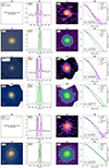Fig. C.1. Continued (5/8).

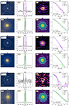Fig. C.1. Continued (6/8).

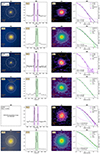Fig. C.1. Continued (7/8).

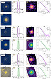Fig. C.1. Continued (8/8).

Appendix D: Correlations between spatial offset and size

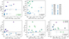Fig. D.1. Relation between the Mg II and [O II] spatial extent and offset measured for our sample. Top left (right): Mg II ([O II]) exponential scale length plotted as a function of the Mg II ([O II]) spatial offset relative to the continuum. Bottom left (middle): Ratio between the Mg II ([O II]) and continuum scale length versus the Mg II ([O II]) spatial offset relative to the continuum. Bottom right: Ratio between the Mg II and [O II] scale length versus the Mg II spatial offset relative to the [O II] emission. The Kendall correlation coefficient (τ) and the corresponding probability that the correlation is real (p) are given and colored in green if the correlation is statistically significant (Akritas & Siebert 1996; Flury et al. 2022b, see Sect. 3.4). Objects with statistically significant Mg II and [O II] extended emission are indicated by large purple and green symbols, respectively (Sect. 3.4).

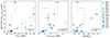Fig. D.2. Relation between the Mg II – continuum spatial offsets and the [O II] (left) and continuum (middle) exponential scale lengths, as well as the UV half-light radii (right). The Kendall correlation coefficient (τ) and the corresponding probability that the correlation is real (p) are given and colored in green if the correlation is statistically significant (Akritas & Siebert 1996; Flury et al. 2022b, see Sect. 3.4).

Appendix E: Correlations between $f_{\mathrm{esc}}^{\mathrm{LyC}}$ and the nebular to continuum scale length ratio

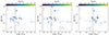Fig. E.1. $f_{\mathrm{esc}}^{\mathrm{LyC}}$ as a function of the ratio of the Mg II ([O II]) scale length to continuum scale length is shown in the left (middle) panel. The right panel shows $f_{\mathrm{esc}}^{\mathrm{LyC}}$ versus the Mg II and [O II] scale length ratio. Objects with upper limits for both scale lengths are shown at x = 0 with red lower limits and higher transparency.

All Tables

All Figures

Fig. 1. Selection of our diverse sample of LyC leakers (pink) from the Izotov et al. (2022, green) and LzLCS+ (black; Izotov et al. 2016a,b, 2018a,b, 2021; Wang et al. 2019; Flury et al. 2022a) samples. The x- and y- axis show the redshift and LyC escape fraction derived in the literature from fitting the COS UV spectrum, respectively (see Sect. 2.1). The triangle symbols show the $f_{\mathrm{esc}}^{\mathrm{LyC}}$ upper limits for the different samples. The dashed and dotted lines indicate the redshift corresponding to the wavelength cutoff of KCWI (λ = 3500 Å) and LRS2 (λ = 3650 Å), respectively. We show the redshift and $f_{\mathrm{esc}}^{\mathrm{LyC}}$ distributions at the top and right of the figure, respectively.

In the text

Fig. 2. Example of a LyC leaking source (J1243+4646, $f_{\mathrm{esc}}^{\mathrm{LyC}}=0.889$) from our sample observed with KCWI. (a) 5″ × 5″ HST/COS acquisition image (when available) plotted with a power-law stretch. The circle indicates the 2$\stackrel{″}{.}$5 COS spectroscopic aperture (diameter). This aperture is also shown on the white light image e and was used to integrate the spectrum shown in panels b and f for comparison. (b) Observed Mg II line doublet extracted in a 2$\stackrel{″}{.}$5 aperture (units of erg s−1 cm−2 Å−1). The purple areas show the narrow band (NB) image spectral coverage. The vertical lines indicate the systemic redshift from Flury et al. (2022a) and Izotov et al. (2022). (c) 5″ × 5″ Mg II NB image plotted with a power-law stretch. The white contours correspond to Mg II significance levels of 3, 6 and 9σ (solid, dashed, and dotted, respectively). The blue circle shows the PSF FWHM estimated at Mg II wavelengths. The “+” and “x” symbols show the best-fit centroids of the emission line and nearby continuum, respectively. If neighboring sources were masked for the analysis, the mask is shown with an orange contour. (d) Radial surface brightness (SB) profiles of the observed and modeled Mg II emission (purple dots and line, resp.) compared to the modeled continuum (black) and PSF (blue) estimated at Mg II wavelengths. If the source is unresolved, the blue and black lines are under the purple or green line. The 3σ SB limit is shown as a dotted line. The shaded area represents the 1σ uncertainties from bootstrapping analysis. The horizontal error bars corresponds to the annulus width used to build the profiles. (e) IFU white light image. (f) [O II] line doublet (units of erg s−1 cm−2 Å−1). (g) Same as (c) for [O II]. (h) Same as (d) for [O II].

In the text

	Fig. 3. Same as Fig. 2 but showing one object (J1517+3705, $f_{\mathrm{esc}}^{\mathrm{LyC}}=0.04$) observed with LRS2. The size of the images is 10″ × 10″. The white areas are regions on the sky uncovered by our detector.
In the text

Fig. 4. Comparisons of the spatial scale lengths (rs) as measured in Sect. 3.3: Mg II and continuum (left), [O II] and continuum (middle), and Mg II and [O II] (right). Objects with statistically significant Mg II and [O II] extended emission compared to continuum are indicated by large purple and green symbols, respectively (Sect. 3.4). Gray symbols in the right panel result in the overlap of the purple and green symbols and thus indicate that both Mg II and [O II] halos are detected. The dotted lines show by how much on average the emission is statistically more extended compared to the continuum (or emission) scale lengths: median ∼1.4 times for Mg II and ∼1.5 times for [O II] compared to the continuum, and 1.2 for the Mg II/[O II] ratio. The black line shows the 1:1 relation (i.e., no extended emission). Upper/lower limit values are shown with arrows. The Kendall correlation coefficient (τ) for every pair of variables and the corresponding false-positive probability that the correlation is real (p) are given and colored in green if the correlation is > 2σ statistically significant (Akritas & Siebert 1996; Flury et al. 2022b, see Sect. 3.4).

In the text

Fig. 5. Relation between the LyC escape fraction and the spatial extent of the neutral and/or low-ionization (left panel) and ionized gas (right panel) as traced by the Mg II and [O II] scale lengths, respectively. The points are color-coded by the O32 values measured in Flury et al. (2022a). Objects with undetected Mg II are shown with higher transparency at x = 0. The red squares indicate the fraction of strong LyC leakers (5σ detection and $f_{\mathrm{esc}}^{\mathrm{LyC}}>5\%$ following Flury et al. 2022a) detected in the bin delimited by the horizontal error bars. The errors on the fractions correspond to a 1σ confidence interval (see Sect. 5.1). While weak and non LyC emitters show a wide diversity of Mg II and [O II] spatial extents, the neutral and/or low-ionization and ionized gas of strong leakers is compact (see Sects. 4.1 and 5.3).

In the text

Fig. 6. Relation between the LyC escape fraction and the spatial offset of the neutral and/or low-ionization (as traced by Mg II, Δ[Mg II]−cont, left panel) and ionized gas (as traced by [O II], Δ[O II]−cont, middle panel) from the stellar continuum. The right panel shows $f_{\mathrm{esc}}^{\mathrm{LyC}}$ as a function of the Mg II spatial offset relative to the [O II] centroid (ΔMg II−[O II]). The red squares indicate the fraction of strong LyC leakers detected in the bin shown by the horizontal error bars. The errors on the fractions correspond to a 1σ confidence interval (see Sect. 4.1). Symbols legend is the same as Fig. 5. While weak and non LyC emitters show a wide diversity of Mg II and [O II] spatial offset from the continuum, leakers have no/weak offset due to their compact configurations (see Sect. 4.1).

In the text

Fig. 7. Composite images of our strong ($f_{\mathrm{esc}}^{\mathrm{LyC}}>4\%$, top row) and non and weak ($f_{\mathrm{esc}}^{\mathrm{LyC}}<4\%$, middle row) LyC leakers observed with KCWI (see Sect. 4.3). The UV continuum, Mg II and [O II] mean stacks are shown from left to right, respectively. The contours are spaced logarithmically by 0.2 dex, with the lowest contour level always at 4 × 10−18 erg s−1 cm−2 arcsec−2. The bottom row compares the continuum (left), Mg II (middle) and [O II] (right) radial SB profiles of the two subsets composites images. In each bottom panels, the lighter (darker) colored profiles with square (circle) symbols correspond to the strong (non/weak) LyC leaker subsample. The full and empty markers show the profiles of the median and mean composite images, respectively. The dotted lines correspond to the SB profiles of the median stacked PSF images of the different subsamples. The dashed lines show the 2σ significance levels.

In the text

	Fig. 8. Direct comparison between the radial SB profiles of the strong ($f_{\mathrm{esc}}^{\mathrm{LyC}}>4\%$, top) and weak and non ($f_{\mathrm{esc}}^{\mathrm{LyC}}<4\%$, bottom) LyC leakers composite images. The legend is the same as in Fig. 7.
In the text

Fig. 9. Comparisons of the emission scale lengths (Mg II in purple and [O II] in green) and the O32 ratios (top left), Hβ equivalent widths (top middle), metallicities (top right), UV half-light radii (bottom left), and H I covering fractions (bottom right). Upper limit values are shown with arrows. The Kendall correlation coefficient (τ) for every pair of variables and the corresponding false-positive probability that the correlation is real (p) are given for both emission lines in the top right corners following the same color coding as the data points (Akritas & Siebert 1996; Flury et al. 2022b, see Sect. 3.4).

In the text

Fig. B.1. Characterization of the KCWI point spread function. Example for the standard star (Feige66) where the first and second rows show the size measurement at Mg II (≈ 3790 Å) and [O II] (≈ 5045 Å) wavelengths of the corresponding science object observed (J1256+4509), respectively. First panel: Narrow-band image at the wavelengths of interest (≈ 1000 km s−1 wide or 13 Å at z = 0.35). The white and orange contours corresponds to SB levels of 10−14, 10−13, and 10−12 erg s−1 cm−2 arcsec−2 for the data and Moffat best-fit model, respectively. Second panel: Fit residuals of the Moffat best-fit model. Third panel: Radial SB profiles of the standard star data (black), Gaussian best-fit model (blue) and Moffat best-fit model (orange). The best-fit model parameters are shown in the bottom left. Forth panel: Zoom-in on the inner profiles. A Moffat model better describes both the core and wings of the PSF for our KCWI observations.

In the text

Fig. B.2. Same as Fig. B.1 but for the LRS2 PSF characterization. We show the size measurements of the standard star BD+210607 observed at the end of the night of the J0804+4726 observations. We do not include a rotation measurement because most of the standards stars can be considered as circular (see Fig. B.3). The size of the stars as observed with LRS2 and therefore the LRS2 PSF is better described with a Moffat model.

In the text

Fig. B.3. LRS2 PSF shape and estimation of its FWHM based on the DIMM seeing. Left panel: Distribution of the FWHM PSF ratio, Q(FWHM) = FWHMX/FWHMY, measured on the standard stars observed with LRS2. The PSF is on average consistent with being circular with a mean FWHM ratio of 0.97±0.08. Second left to right: Comparison between the DIMM seeing at the telescope and the FWHM (mean between the x- and y-axis of the elliptical Moffat function, see Fig. B.2) measured on the standard stars (Sect. B.2) at the middle of the LRS2-B wavelength window (∼ 5300 Å), at the Mg II and at the [O II] wavelengths, respectively. The dashed line shows the one-to-one relation. The DIMM seeing provides a relatively good estimation of the PSF FWHM near ∼ 5300 Å but overestimates it at Mg II wavelengths (≈ 3780 Å). The red line shows the estimated PSF FWHM based on the DIMM seeing calculated using Eq. B.1 (see Sect. B.2).

In the text

Fig. B.4. First panel: Evolution of the PSF FWHM with wavelength for the standard star BD+210607 observed with LRS2. The vertical dashed line indicate the Mg II and [O II] wavelengths of the science object J080425+472607. The vertical dotted blue line corresponds to the central wavelength of LRS2B (≈ 5300 Å). The solid blue line shows the best first-order polynomial fit to the data. The resulting slope is −9 × 10−5 which is consistent with the average value obtained from all the standard stars (middle and right panels). Second panel: Best first-order polynomial fits of the PSF FWHM – wavelength relation of all the standard stars (gray). The relation resulting from the median slope and the standard deviation is shown with solid and dotted black line, respectively. Third panel: Distribution of the slope measured on the standard stars. The solid and dotted vertical lines indicate the median and standard deviation of the distribution (values on middle right), respectively. Fourth panel: Evolution of the Moffat β parameter with wavelength for all the standard stars (gray). The empty squares and corresponding errorbars give the median value and median absolute deviation in each wavelength bin. The blue dots show the BD+210607 values.

In the text

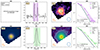	Fig. C.1. Same as Fig. 2 (Part 1/8).
In the text

	Fig. C.1. Continued (2/8).
In the text

	Fig. C.1. Continued (3/8).
In the text

	Fig. C.1. Continued (4/8).
In the text

	Fig. C.1. Continued (5/8).
In the text

	Fig. C.1. Continued (6/8).
In the text

	Fig. C.1. Continued (7/8).
In the text

	Fig. C.1. Continued (8/8).
In the text

Fig. D.1. Relation between the Mg II and [O II] spatial extent and offset measured for our sample. Top left (right): Mg II ([O II]) exponential scale length plotted as a function of the Mg II ([O II]) spatial offset relative to the continuum. Bottom left (middle): Ratio between the Mg II ([O II]) and continuum scale length versus the Mg II ([O II]) spatial offset relative to the continuum. Bottom right: Ratio between the Mg II and [O II] scale length versus the Mg II spatial offset relative to the [O II] emission. The Kendall correlation coefficient (τ) and the corresponding probability that the correlation is real (p) are given and colored in green if the correlation is statistically significant (Akritas & Siebert 1996; Flury et al. 2022b, see Sect. 3.4). Objects with statistically significant Mg II and [O II] extended emission are indicated by large purple and green symbols, respectively (Sect. 3.4).

In the text

Fig. D.2. Relation between the Mg II – continuum spatial offsets and the [O II] (left) and continuum (middle) exponential scale lengths, as well as the UV half-light radii (right). The Kendall correlation coefficient (τ) and the corresponding probability that the correlation is real (p) are given and colored in green if the correlation is statistically significant (Akritas & Siebert 1996; Flury et al. 2022b, see Sect. 3.4).

In the text

	Fig. E.1. $f_{\mathrm{esc}}^{\mathrm{LyC}}$ as a function of the ratio of the Mg II ([O II]) scale length to continuum scale length is shown in the left (middle) panel. The right panel shows $f_{\mathrm{esc}}^{\mathrm{LyC}}$ versus the Mg II and [O II] scale length ratio. Objects with upper limits for both scale lengths are shown at x = 0 with red lower limits and higher transparency.
In the text

References

- Akritas, M. G., & Siebert, J. 1996, MNRAS, 278, 919 [NASA ADS] [CrossRef] [Google Scholar]
- Amorín, R., Pérez-Montero, E., Vílchez, J. M., & Papaderos, P. 2012, ApJ, 749, 185 [CrossRef] [Google Scholar]
- Amorín, R. O., Rodríguez-Henríquez, M., Fernández, V., et al. 2024, A&A, 682, L25 [NASA ADS] [CrossRef] [EDP Sciences] [Google Scholar]
- Arribas, S., Perna, M., Rodríguez Del Pino, B., et al. 2024, A&A, in press, https://doi.org/10.1051/0004-6361/202348824 [Google Scholar]
- Bacon, R., Accardo, M., Adjali, L., et al. 2010, Proc. SPIE, 7735, 773508 [Google Scholar]
- Bañados, E., Venemans, B. P., Mazzucchelli, C., et al. 2018, Nature, 553, 473 [Google Scholar]
- Becker, R. H., Fan, X., White, R. L., et al. 2001, AJ, 122, 2850 [NASA ADS] [CrossRef] [Google Scholar]
- Begley, R., Cullen, F., McLure, R. J., et al. 2024, MNRAS, 527, 4040 [Google Scholar]
- Borthakur, S., Heckman, T. M., Leitherer, C., & Overzier, R. A. 2014, Science, 346, 216 [Google Scholar]
- Bosman, S. E. I., Davies, F. B., Becker, G. D., et al. 2022, MNRAS, 514, 55 [NASA ADS] [CrossRef] [Google Scholar]
- Bouché, N., Murphy, M. T., Péroux, C., Csabai, I., & Wild, V. 2006, MNRAS, 371, 495 [CrossRef] [Google Scholar]
- Bouché, N., Murphy, M. T., Péroux, C., et al. 2007, ApJ, 669, L5 [CrossRef] [Google Scholar]
- Bouché, N., Hohensee, W., Vargas, R., et al. 2012, MNRAS, 426, 801 [CrossRef] [Google Scholar]
- Bouwens, R., Illingworth, G., Oesch, P., et al. 2023, MNRAS, 523, 1009 [NASA ADS] [CrossRef] [Google Scholar]
- Bunker, A. J., Saxena, A., Cameron, A. J., et al. 2023, A&A, 677, A88 [NASA ADS] [CrossRef] [EDP Sciences] [Google Scholar]
- Burchett, J. N., Rubin, K. H. R., Prochaska, J. X., et al. 2021, ApJ, 909, 151 [NASA ADS] [CrossRef] [Google Scholar]
- Cameron, A. J., Saxena, A., Bunker, A. J., et al. 2023, A&A, 677, A115 [NASA ADS] [CrossRef] [EDP Sciences] [Google Scholar]
- Carr, C., Scarlata, C., Henry, A., & Panagia, N. 2021, ApJ, 906, 104 [NASA ADS] [CrossRef] [Google Scholar]
- Casey, C. M., Akins, H. B., Shuntov, M., et al. 2024, ApJ, 965, 98 [NASA ADS] [CrossRef] [Google Scholar]
- Cen, R., & Kimm, T. 2015, ApJ, 801, L25 [Google Scholar]
- Chisholm, J., Orlitová, I., Schaerer, D., et al. 2017, A&A, 605, A67 [NASA ADS] [CrossRef] [EDP Sciences] [Google Scholar]
- Chisholm, J., Prochaska, J. X., Schaerer, D., Gazagnes, S., & Henry, A. 2020, MNRAS, 498, 2554 [CrossRef] [Google Scholar]
- Chonis, T. S., Hill, G. J., Lee, H., et al. 2016, in Ground-based and Airborne Instrumentation for Astronomy VI, eds. C. J. Evans, L. Simard, & H. Takami, SPIE Conf. Ser., 9908, 99084C [NASA ADS] [Google Scholar]
- Choustikov, N., Katz, H., Saxena, A., et al. 2024, MNRAS, submitted [arXiv:2401.09557] [Google Scholar]
- Claeyssens, A., Richard, J., Blaizot, J., et al. 2022, A&A, 666, A78 [NASA ADS] [CrossRef] [EDP Sciences] [Google Scholar]
- Dayal, P., Volonteri, M., Greene, J. E., et al. 2024, A&A, submitted [arXiv:2401.11242] [Google Scholar]
- Dutta, R., Fumagalli, M., Fossati, M., et al. 2020, MNRAS, 499, 5022 [CrossRef] [Google Scholar]
- Dutta, R., Fossati, M., Fumagalli, M., et al. 2023, MNRAS, 522, 535 [NASA ADS] [CrossRef] [Google Scholar]
- Endsley, R., Stark, D. P., Chevallard, J., & Charlot, S. 2021, MNRAS, 500, 5229 [Google Scholar]
- Fan, X., Strauss, M. A., Becker, R. H., et al. 2006, AJ, 132, 117 [NASA ADS] [CrossRef] [Google Scholar]
- Finkelstein, S. L., Ryan, R. E., Papovich, C., et al. 2015, ApJ, 810, 71 [NASA ADS] [CrossRef] [Google Scholar]
- Finkelstein, S. L., D’Aloisio, A., Paardekooper, J.-P., et al. 2019, ApJ, 879, 36 [Google Scholar]
- Finley, H., Bouché, N., Contini, T., et al. 2017, A&A, 608, A7 [NASA ADS] [CrossRef] [EDP Sciences] [Google Scholar]
- Flury, S. R., Jaskot, A. E., Ferguson, H. C., et al. 2022a, ApJS, 260, 1 [NASA ADS] [CrossRef] [Google Scholar]
- Flury, S. R., Jaskot, A. E., Ferguson, H. C., et al. 2022b, ApJ, 930, 126 [NASA ADS] [CrossRef] [Google Scholar]
- Garel, T., Blaizot, J., Rosdahl, J., et al. 2021, MNRAS, 504, 1902 [NASA ADS] [CrossRef] [Google Scholar]
- Gazagnes, S., Chisholm, J., Schaerer, D., et al. 2018, A&A, 616, A29 [NASA ADS] [CrossRef] [EDP Sciences] [Google Scholar]
- Gazagnes, S., Chisholm, J., Schaerer, D., Verhamme, A., & Izotov, Y. 2020, A&A, 639, A85 [NASA ADS] [CrossRef] [EDP Sciences] [Google Scholar]
- Gebhardt, K., Mentuch Cooper, E., Ciardullo, R., et al. 2021, ApJ, 923, 217 [NASA ADS] [CrossRef] [Google Scholar]
- Goulding, A. D., Greene, J. E., Setton, D. J., et al. 2023, ApJ, 955, L24 [NASA ADS] [CrossRef] [Google Scholar]
- Grazian, A., Giallongo, E., Boutsia, K., et al. 2022, ApJ, 924, 62 [NASA ADS] [CrossRef] [Google Scholar]
- Grazian, A., Boutsia, K., Giallongo, E., et al. 2023, ApJ, 955, 60 [NASA ADS] [CrossRef] [Google Scholar]
- Guo, Y., Bacon, R., Bouché, N. F., et al. 2023, Nature, 624, 53 [NASA ADS] [CrossRef] [Google Scholar]
- Hayes, M., Östlin, G., Schaerer, D., et al. 2013, ApJ, 765, L27 [NASA ADS] [CrossRef] [Google Scholar]
- Henry, A., Berg, D. A., Scarlata, C., Verhamme, A., & Erb, D. 2018, ApJ, 855, 96 [Google Scholar]
- Herenz, E. C., & Wisotzki, L. 2017, A&A, 602, A111 [NASA ADS] [CrossRef] [EDP Sciences] [Google Scholar]
- Hill, G. J., Lee, H., MacQueen, P. J., et al. 2021, AJ, 162, 298 [NASA ADS] [CrossRef] [Google Scholar]
- Ho, S. H., Martin, C. L., Kacprzak, G. G., & Churchill, C. W. 2017, ApJ, 835, 267 [NASA ADS] [CrossRef] [Google Scholar]
- Inoue, A. K., Shimizu, I., Iwata, I., & Tanaka, M. 2014, MNRAS, 442, 1805 [NASA ADS] [CrossRef] [Google Scholar]
- Inoue, A. K., Hasegawa, K., Ishiyama, T., et al. 2018, PASJ, 70, 55 [Google Scholar]
- Izotov, Y. I., Orlitová, I., Schaerer, D., et al. 2016a, Nature, 529, 178 [Google Scholar]
- Izotov, Y. I., Schaerer, D., Thuan, T. X., et al. 2016b, MNRAS, 461, 3683 [Google Scholar]
- Izotov, Y. I., Schaerer, D., Worseck, G., et al. 2018a, MNRAS, 474, 4514 [Google Scholar]
- Izotov, Y. I., Worseck, G., Schaerer, D., et al. 2018b, MNRAS, 478, 4851 [Google Scholar]
- Izotov, Y. I., Worseck, G., Schaerer, D., et al. 2021, MNRAS, 503, 1734 [NASA ADS] [CrossRef] [Google Scholar]
- Izotov, Y. I., Chisholm, J., Worseck, G., et al. 2022, MNRAS, 515, 2864 [NASA ADS] [CrossRef] [Google Scholar]
- Jaskot, A. E., & Oey, M. S. 2013, ApJ, 766, 91 [Google Scholar]
- Jaskot, A. E., Oey, M. S., Scarlata, C., & Dowd, T. 2017, ApJ, 851, L9 [NASA ADS] [CrossRef] [Google Scholar]
- Jaskot, A. E., Silveyra, A. C., Plantinga, A., et al. 2024, ApJ, submitted [arXiv:2406.10171] [Google Scholar]
- Kanekar, N., Ghosh, T., Rhoads, J., et al. 2021, ApJ, 913, L15 [NASA ADS] [CrossRef] [Google Scholar]
- Katz, H., Ďurovčíková, D., Kimm, T., et al. 2020, MNRAS, 498, 164 [Google Scholar]
- Kulkarni, G., Keating, L. C., Haehnelt, M. G., et al. 2019a, MNRAS, 485, L24 [Google Scholar]
- Kulkarni, G., Worseck, G., & Hennawi, J. F. 2019b, MNRAS, 488, 1035 [Google Scholar]
- Kusakabe, H., Blaizot, J., Garel, T., et al. 2020, A&A, 638, A12 [NASA ADS] [CrossRef] [EDP Sciences] [Google Scholar]
- Leclercq, F., Bacon, R., Wisotzki, L., et al. 2017, A&A, 608, A8 [NASA ADS] [CrossRef] [EDP Sciences] [Google Scholar]
- Leclercq, F., Bacon, R., Verhamme, A., et al. 2020, A&A, 635, A82 [NASA ADS] [CrossRef] [EDP Sciences] [Google Scholar]
- Leclercq, F., Verhamme, A., Epinat, B., et al. 2022, A&A, 663, A11 [NASA ADS] [CrossRef] [EDP Sciences] [Google Scholar]
- Leitet, E., Bergvall, N., Hayes, M., Linné, S., & Zackrisson, E. 2013, A&A, 553, A106 [NASA ADS] [CrossRef] [EDP Sciences] [Google Scholar]
- Leitherer, C., Hernandez, S., Lee, J. C., & Oey, M. S. 2016, ApJ, 823, 64 [Google Scholar]
- Le Reste, A., Cannon, J. M., Hayes, M. J., et al. 2024, MNRAS, 528, 757 [NASA ADS] [CrossRef] [Google Scholar]
- Lewis, J. S. W., Ocvirk, P., Aubert, D., et al. 2020, MNRAS, 496, 4342 [NASA ADS] [CrossRef] [Google Scholar]
- Lundgren, B. F., Creech, S., Brammer, G., et al. 2021, ApJ, 913, 50 [NASA ADS] [CrossRef] [Google Scholar]
- Madau, P., & Haardt, F. 2015, ApJ, 813, L8 [Google Scholar]
- Marques-Chaves, R., Schaerer, D., Álvarez-Márquez, J., et al. 2021, MNRAS, 507, 524 [NASA ADS] [CrossRef] [Google Scholar]
- Marques-Chaves, R., Schaerer, D., Álvarez-Márquez, J., et al. 2022, MNRAS, 517, 2972 [CrossRef] [Google Scholar]
- Martin, C., Moore, A., Morrissey, P., et al. 2010, in Ground-based and Airborne Instrumentation for Astronomy III, eds. I. S. McLean, S. K. Ramsay, & H. Takami, SPIE Conf. Ser., 7735, 77350M [Google Scholar]
- Mascia, S., Pentericci, L., Calabrò, A., et al. 2023, A&A, 672, A155 [NASA ADS] [CrossRef] [EDP Sciences] [Google Scholar]
- Maseda, M. V., Bacon, R., Lam, D., et al. 2020, MNRAS, 493, 5120 [Google Scholar]
- Mauerhofer, V., Verhamme, A., Blaizot, J., et al. 2021, A&A, 646, A80 [NASA ADS] [CrossRef] [EDP Sciences] [Google Scholar]
- Moffat, A. F. J. 1969, A&A, 3, 455 [NASA ADS] [Google Scholar]
- Morrissey, P., Matuszewski, M., Martin, D. C., et al. 2018, ApJ, 864, 93 [Google Scholar]
- Naidu, R. P., Oesch, P. A., van Dokkum, P., et al. 2022a, ApJ, 940, L14 [NASA ADS] [CrossRef] [Google Scholar]
- Naidu, R. P., Matthee, J., Oesch, P. A., et al. 2022b, MNRAS, 510, 4582 [CrossRef] [Google Scholar]
- Nakajima, K., & Ouchi, M. 2014, MNRAS, 442, 900 [Google Scholar]
- Nelson, D., Byrohl, C., Peroux, C., Rubin, K. H. R., & Burchett, J. N. 2021, MNRAS, 507, 4445 [NASA ADS] [CrossRef] [Google Scholar]
- Newville, M., Stensitzki, T., Allen, D. B., & Ingargiola, A. 2014, https://doi.org/10.5281/zenodo.11813 [Google Scholar]
- Ono, Y., Harikane, Y., Ouchi, M., et al. 2023, ApJ, 951, 72 [NASA ADS] [CrossRef] [Google Scholar]
- Ormerod, K., Conselice, C. J., Adams, N. J., et al. 2024, MNRAS, 527, 6110 [Google Scholar]
- Östlin, G., Hayes, M., Duval, F., et al. 2014, ApJ, 797, 11 [CrossRef] [Google Scholar]
- O’Sullivan, D., & Chen, Y. 2020, arXiv e-prints [arXiv:2011.05444] [Google Scholar]
- Ouchi, M., Mobasher, B., Shimasaku, K., et al. 2009, ApJ, 706, 1136 [NASA ADS] [CrossRef] [Google Scholar]
- Ouchi, M., Harikane, Y., Shibuya, T., et al. 2018, PASJ, 70, S13 [Google Scholar]
- Péroux, C., Rahmani, H., Quiret, S., et al. 2017, MNRAS, 464, 2053 [CrossRef] [Google Scholar]
- Planck Collaboration VI. 2020, A&A, 641, A6 [NASA ADS] [CrossRef] [EDP Sciences] [Google Scholar]
- Rahmani, H., Péroux, C., Augustin, R., et al. 2018, MNRAS, 474, 254 [NASA ADS] [CrossRef] [Google Scholar]
- Ramsey, L. W., Adams, M. T., Barnes, T. G., et al. 1998, in Advanced Technology Optical/IR Telescopes VI, ed. L. M. Stepp, SPIE Conf. Ser., 3352, 34 [NASA ADS] [CrossRef] [Google Scholar]
- Rasekh, A., Melinder, J., Östlin, G., et al. 2022, A&A, 662, A64 [NASA ADS] [CrossRef] [EDP Sciences] [Google Scholar]
- Rinaldi, P., Caputi, K. I., Costantin, L., et al. 2023, ApJ, 952, 143 [NASA ADS] [CrossRef] [Google Scholar]
- Robertson, B. E. 2022, ARA&A, 60, 121 [NASA ADS] [CrossRef] [Google Scholar]
- Robertson, B. E., Ellis, R. S., Furlanetto, S. R., & Dunlop, J. S. 2015, ApJ, 802, L19 [Google Scholar]
- Robertson, B. E., Tacchella, S., Johnson, B. D., et al. 2023, Nat. Astron., 7, 611 [NASA ADS] [CrossRef] [Google Scholar]
- Rosdahl, J., Katz, H., Blaizot, J., et al. 2018, MNRAS, 479, 994 [NASA ADS] [Google Scholar]
- Runnholm, A., Hayes, M. J., Lin, Y.-H., et al. 2023, MNRAS, 522, 4275 [NASA ADS] [CrossRef] [Google Scholar]
- Rupke, D. S. N., Coil, A., Geach, J. E., et al. 2019, Nature, 574, 643 [NASA ADS] [CrossRef] [Google Scholar]
- Saldana-Lopez, A., Schaerer, D., Chisholm, J., et al. 2022, A&A, 663, A59 [NASA ADS] [CrossRef] [EDP Sciences] [Google Scholar]
- Saldana-Lopez, A., Schaerer, D., Chisholm, J., et al. 2023, MNRAS, 522, 6295 [NASA ADS] [CrossRef] [Google Scholar]
- Schroeder, J., Mesinger, A., & Haiman, Z. 2013, MNRAS, 428, 3058 [Google Scholar]
- Schroetter, I., Bouché, N., Wendt, M., et al. 2016, ApJ, 833, 39 [NASA ADS] [CrossRef] [Google Scholar]
- Schroetter, I., Bouché, N. F., Zabl, J., et al. 2019, MNRAS, 490, 4368 [CrossRef] [Google Scholar]
- Shaban, A., Bordoloi, R., Chisholm, J., et al. 2022, ApJ, 936, 77 [NASA ADS] [CrossRef] [Google Scholar]
- Steidel, C. C., Bogosavljević, M., Shapley, A. E., et al. 2011, ApJ, 736, 160 [NASA ADS] [CrossRef] [Google Scholar]
- Steidel, C. C., Bogosavljević, M., Shapley, A. E., et al. 2018, ApJ, 869, 123 [Google Scholar]
- Sugahara, Y., Ouchi, M., Harikane, Y., et al. 2019, ApJ, 886, 29 [Google Scholar]
- Trebitsch, M., Blaizot, J., Rosdahl, J., Devriendt, J., & Slyz, A. 2017, MNRAS, 470, 224 [Google Scholar]
- Trebitsch, M., Dubois, Y., Volonteri, M., et al. 2021, A&A, 653, A154 [NASA ADS] [CrossRef] [EDP Sciences] [Google Scholar]
- Tumlinson, J., Peeples, M. S., & Werk, J. K. 2017, ARA&A, 55, 389 [Google Scholar]
- Verhamme, A., Orlitová, I., Schaerer, D., et al. 2017, A&A, 597, A13 [NASA ADS] [CrossRef] [EDP Sciences] [Google Scholar]
- Wang, B., Heckman, T. M., Leitherer, C., et al. 2019, ApJ, 885, 57 [NASA ADS] [CrossRef] [Google Scholar]
- Wisotzki, L., Bacon, R., Blaizot, J., et al. 2016, A&A, 587, A98 [NASA ADS] [CrossRef] [EDP Sciences] [Google Scholar]
- Wisotzki, L., Bacon, R., Brinchmann, J., et al. 2018, Nature, 563, E31 [NASA ADS] [CrossRef] [Google Scholar]
- Wilson, E. B. 1927, JASA, 22, 209 [Google Scholar]
- Xu, X., Henry, A., Heckman, T., et al. 2022, ApJ, 933, 202 [NASA ADS] [CrossRef] [Google Scholar]
- Xu, X., Henry, A., Heckman, T., et al. 2023a, ApJ, 943, 94 [NASA ADS] [CrossRef] [Google Scholar]
- Xu, Y., Ouchi, M., Nakajima, K., et al. 2023b, ApJ, submitted [arXiv:2310.06614] [Google Scholar]
- Yang, L., Morishita, T., Leethochawalit, N., et al. 2022, ApJ, 938, L17 [NASA ADS] [CrossRef] [Google Scholar]
- Zabl, J., Bouché, N. F., Schroetter, I., et al. 2019, MNRAS, 485, 1961 [NASA ADS] [CrossRef] [Google Scholar]
- Zabl, J., Bouché, N. F., Wisotzki, L., et al. 2021, MNRAS, 507, 4294 [NASA ADS] [CrossRef] [Google Scholar]