| Issue |
A&A
Volume 677, September 2023
|
|
|---|---|---|
| Article Number | A137 | |
| Number of page(s) | 60 | |
| Section | Catalogs and data | |
| DOI | https://doi.org/10.1051/0004-6361/202346759 | |
| Published online | 20 September 2023 | |
Stellar variability in Gaia DR3
I. Three-band photometric dispersions for 145 million sources★
1
Centro de Astrobiología. CSIC-INTA, Campus ESAC,
C. bajo del castillo s/n,
28692
Villanueva de la Cañada, Madrid, Spain
e-mail: jmaiz@cab.inta-csic.es
2
Departamento de Astrofísica y Física de la Atmósfera, Universidad Complutense de Madrid,
28040
Madrid, Spain
Received:
27
April
2023
Accepted:
7
August
2023
Context. The unparalleled characteristics of Gaia photometry in terms of calibration, stability, time span, dynamic range, full-sky coverage, and complementary information make it an excellent choice to study stellar variability.
Aims. We aim to measure the photometric dispersion in the G, GBP, and GRP bands of the 145 677 450 third Gaia data release (DR3) five-parameter sources with G ≤ 17 mag and GBP – GRP between −1.0 and 8.0 mag. We will use that unbiased sample to analyze stellar variability in the Milky Way (MW), Large Magellanic Cloud (LMC), and Small Magellanic Cloud (SMC).
Methods. For each band we convert from magnitude uncertainties to observed photometric dispersions, calculate the instrumental component as a function of apparent magnitude and color, and use it to transform the observed dispersions into the astrophysical ones: sG, SGBP, and SGRP. We give variability indices in the three bands for the whole sample indicating whether the objects are non-variable, marginally variable, or clearly so. We use the subsample established by Rimoldini and collaborators with light curves and variability types to calibrate our results and establish their limitations.
Results. The position of an object in the dispersion-dispersion planes can be used to constrain its variability type, a direct application of these results. We use information from the MW, LMC, and SMC color-absolute magnitude diagrams (CAMDs) to discuss variability across the Hertzsprung-Russell diagram. White dwarfs and B-type subdwarfs are more variable than main sequence (MS) or red clump (RC) stars, with a flat distribution in sG up to 10 mmag and with variability decreasing for the former with age. The MS region in the Gaia CAMD includes a mixture of populations from the MS itself and from other evolutionary phases. Its sG distribution peaks at low values (~1–2 mmag) but it has a large tail dominated by eclipsing binaries, RR Lyrae stars, and young stellar objects. RC stars are characterized by little variability, with their sG distribution peaking at 1 mmag or less. The stars in the pre-main-sequence (PMS) region are highly variable, with a power law distribution in sG with slope 2.75 and a cutoff for values lower than 7 mmag. The luminous red stars region of the Gaia CAMD has the highest variability, with its extreme dominated by AGB stars and with a power law in sG with slope ~2.2 that extends from there to a cutoff of 7 mmag. We show that our method can be used to search for LMC Cepheids. We analyze four stellar clusters with O stars (Villafranca O-016, O-021, O-024, and O-026) and detect a strong difference in sG between stars that are already in the MS and those that are still in the PMS.
Key words: stars: variables: general / techniques: photometric / Galaxy: general / Magellanic Clouds
The main table of this paper, as described in Sect. 2.3, is available at the CDS via anonymous ftp to cdsarc.cds.unistra.fr (130.79.128.5) or via https://cdsarc.cds.unistra.fr/viz-bin/cat/J/A+A/677/A137
© The Authors 2023
 Open Access article, published by EDP Sciences, under the terms of the Creative Commons Attribution License (https://creativecommons.org/licenses/by/4.0), which permits unrestricted use, distribution, and reproduction in any medium, provided the original work is properly cited.
This article is published in open access under the Subscribe to Open model. Subscribe to A&A to support open access publication.
1 Introduction
The Gaia mission (Prusti et al. 2016) is arguably the best example of the paradigm change that large-scale surveys have introduced in astronomy. Not long ago, most astronomical research was carried on by individuals or small groups going on observing runs and conducting analyses of one to several hundreds of objects using their own reduction. Such programs are still carried on today and are useful and necessary, but the weight in astronomy has shifted towards large-scale surveys that cover the whole sky or a significant fraction of it, are conducted by large teams, involve samples several orders of magnitude larger, and are reduced using common procedures that ease calibration.
The (full) third Gaia data release (DR3) provides astrometric, photometric, and spectroscopic data for 1.8 × 10⁹ sources (Vallenari et al. 2023). One of the novelties of DR3 is the inclusion of a significantly larger amount of photometric variability information with respect to previous releases: over 12 million sources (less than 1% of the full sample) in the form of epoch photometry and variability classifications (Eyer et al. 2023). The classifications based on the light curves are given by Rimoldini et al. (2023), from now on R23. For the specific case of the 2+ million eclipsing binaries, see Mowlavi et al. (2023). The R23 sample was selected from sources expected to be variable, so it is biased in that sense, something we will verify in this paper.
The quality and quantity of information provided by Gaia allows for a limited analysis of photometric variability without the use of light curves but based instead on the observed photometric dispersions. Previous papers have done that (Deason et al. 2017; Belokurov et al. 2017; Iorio et al. 2018; Vioque et al. 2020; Guidry et al. 2021; Mowlavi et al. 2021; Andrew et al. 2021; Barlow et al. 2022; Barber & Mann 2023) but they have not exploited the full potential provided by using a large fraction of the Gaia DR3 sample, as some of those use previous data releases and others use relatively small samples. That is the purpose of this paper: to calculate astrophysical photometric dispersions for the majority of Gaia DR3 objects with G ≤ 17 mag. We will follow it up with papers on short-timescale variables (Maíz Apellániz et al., in prep.) and with an analysis of the Gaia DR3 light curves for Galactic O stars (Holgado et al., in prep.). Possible topics for future papers include the photometric variability of massive stars, the study of low-mass stars targeted by radial-velocity planet surveys, and an analysis of luminous red stars in the Magellanic Clouds.
In Sect. 2 we present our sample selection and methodology. In Sect. 3 we give our general results for variability across the Gaia color-absolute magnitude diagram (CAMD), in Sect. 4 we discuss some examples of applications of the data presented in this paper, and we end with a summary in Sect. 5.
2 Data and methods
2.1 Sample selection
We started by querying the Gaia DR3 catalog for all sources with (a) G ≤ 17 mag, (b) five-parameter astrometric solutions, and (c) GBP – Grp between −1.0 and 8.0 mag. The reason for constraining the sample in magnitude is that fainter sources have larger instrumental photometric dispersions (see below), thus limiting the usefulness of a variability analysis. In addition, the primary interest of this analysis is stellar variability and the fainter range sampled by Gaia has a larger fraction of QSOs and galaxies. The exclusion of six-parameter solutions is due to their generally poorer photometric quality and our desire to keep a sample with uniform properties. In any case, the proportion of six-parameter solutions for G ≤ 17 mag is small except for the brightest stars (see Fig. 12 in Lindegren et al. 2021b). The third condition only removes a small number of stars, as bluer stars do not exist in theory (one object excluded) and redder stars are scarce and have in general poor astrometry (74 objects excluded). The query resulted in 145 677 450 objects (8% of the total Gaia DR3 sample) and their density distribution in G vs. GBP – GRP is shown in Fig. 1.
In addition, we also queried the Gaia DR3 catalog for light curve and variability information on the sample. 4 991 335 objects (3.426%) have epoch photometry, 4795431 (3.292%) are tagged as variable, and 4 482 655 (3.077%) have a variability classification by R23. We list in Table 1 the breakdown by variable type and we refer to that table and to R23 for the meaning of the acronyms used for each type.
2.2 Parameter calculation
The published Gaia DR3 magnitudes are the weighted averages of a large number of individual measurements. Two measurements of the same star are not identical due to a combination of instrumental and astrophysical (or intrinsic) variability. The first one can be approximated as a Gaussian distribution, keeping in mind the possibility of outliers (an issue we come back to below). As for the astrophysical variability, the measured magnitudes can have quite different distributions, from symmetrical but non-Gaussian in cases such as ellipsoidal variables to asymmetrical in most eclipsing binaries or bursting sources. However, under the reasonable assumption that both are independent, the relationship between the observed dispersion sX,0 and the astro-physical sX and instrumental sX,ins dispersions for a band X (G, GBP, or GRP) is given by:

where sX,0 itself is the product of the listed magnitude uncertainty σX by  . NX is the number of observations used for photometry, as σX is the (weighted) standard deviation of the mean of the distribution (Eq. (5) in Riello et al. 2021).
The obvious interest is the determination of the astrophys-ical dispersions sG,  , and
, and  , which requires the prior calculation of the instrumental component to be subtracted in quadrature. Those components are primarily a function of magnitude (Riello et al. 2021) but can also depend on other parameters such as color. Given the behavior seen in Fig. 14 of Riello et al. (2021) and our equivalent Fig. 2 (see also the plots in Appendix E of R23), we proceeded in the following way:
We divided the sample in G-magnitude bins between 3 mag and 17 mag in order to capture the trends seen in Fig. 2. In particular, the observed dispersions decrease as G increases for bright stars, then become relatively flat (but with some fine structure) for a range of intermediate values of G (between 7 mag and 13 mag, approximately), and finally increase between G of 13 mag and 17 mag. The behavior in the last section is the typical one caused by an increase in Poisson noise as stars become fainter. The behavior in the first two is caused by the complexities of the Gaia CCD observations, including the use of different gate configurations as a function of magnitude (Carrasco et al. 2016). The 20 magnitude bins are selected to trace the structures seen in Fig. 2.
We also divided the sample in five GBP – GRP bins to capture the differences as a function of color, yielding a total of 100 magnitude-color bins (Fig. 1). We selected the limits at GBP – GRP of 0.2, 1.0, 1.5, and 2.5 mag for several reasons, the main one being that we tested several options and those where the ones that better captured the changes in behavior as a function of color while being representative of the different values of the effective wavenumber that is used for astrometry (see Fig. 2 in Lindegren et al. 2021a). In addition, the five ranges sample different astrophysical populations that are mixed to a degree by extinction. The first range includes OBA stars, subdwarfs, and WDs. We note that most Galactic OB stars are driven out of it by extinction, leaving mostly massive stars in the Magellanic Clouds in it. The second range is dominated by FG stars in the main sequence (MS) and the third one by somewhat later (or more extinguished) MS stars but also a significant fraction of red clump (RC) stars, The fourth and fifth include a mixed bag of extinguished versions of the above, M dwarfs, red giants, AGB stars, and YSOs, with the main difference between the two ranges being caused by extinction.
-
For each of those magnitude-color bins we assumed that the distribution of astrophysical dispersions is given by a functional form:
where A is a normalizing constant, α is the exponent that characterizes a power-law behavior at large values of the dispersion, and sx,c is a characteristic value where the distribution flattens to adjust the proportion between low-dispersion and high-dispersion values. Below we discuss how well this model describes reality.
-
The instrumental dispersion sX,ins in a given magnitude-color bin can be characterized by a Gaussian average value sX,i and a width σΧ,ί. The explanation for such a width is that even if we make the bins relatively small, a given sample is bound to contain objects with a range of magnitudes, colors, and number of observations (among other characteristics) that generate slightly different instrumental effects. We used σX,i as the uncertainty on sX,i when computing sX with Eq. (1). The distribution of total dispersions is formed then by convolving Eq. (2) with the Gaussian distribution in SX,ins:
with sX obtained from Eq. (1) and where we verified that σX,i ≪ sX,i for all magnitude-color bins in order to avoid a significant contribution from the unphysical range sX,ins > sX,0.


The above procedure led us to fit the distribution of observed dispersions in each magnitude-color bin with a function of five parameters: A, sX,c, α, sX,i, and σX,i. We wrote an IDL procedure to do the fits and the results are listed in Tables B.1–B.3, where we give the total number of stars N instead of A as a normalizing constant to ease interpretation. The corresponding plots are shown in Figs. 3 and B.1 (each one of them is a vertical slice of one of the plots in Fig. 2), where we also show the histograms for the three most common variable types and the rest of the variables from R23 in each case, noting that only a fraction of the sample (given in each plot) has a variability type from that paper. The plots are useful to estimate how many of the variable stars are in R23 and which are the dominant types of variables across the Gaia color-magnitude diagram (CMD).
Further below we analyze the distribution of variable stars across the Gaia CAMD but for the time being we stick to the CMD, as our initial purpose is to analyze instrumental effects that depend on magnitude, not on absolute magnitude. We note that the histograms in Fig. B.1 have a constant logarithmic bin size in the x axis. This is done for display purposes but the fits themselves were performed using variable bin sizes that reduce the differences in the number of stars per bin, as using a constant bin size can lead to biases in the fit (Maíz Apellániz & Úbeda 2005), which in this case would affect mostly the value of α.
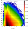 |
Fig. 1 Source density (logarithmic scale) in the color-magnitude plane for the sample in this paper. Dotted black lines indicate the magnitude-color bins used to determine the characteristics of the photometric dispersion. |
Statistics for the stars in the sample with R23 variability classifications.
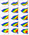 |
Fig. 2 Observed photometric dispersions for G (left column), GBP (center column), and GRP (right column) for the five GBP – GRP ranges used in this work, from top to bottom: −1.0–0.2, 0.2−1.0, 1.0–1.5, 1.5–2.5, and 2.5–8.0 (in mag). The plotted points and error bars are the measurements of the instrumental dispersions sX,i and their widths σX,i for each magnitude bin and the grey line joining them is a cubic spline fit. The horizontal axes are in mag and the vertical ones in mmag. |
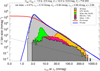 |
Fig. 3 Example of a total dispersion histogram used to calculate the instrumental dispersion as a function of magnitude and color (see Fig. B.1 for the whole set). The histogram has a uniform bin size in logarithmic units (see the text for the bins used for fitting) and both the horizontal and vertical scales are logarithmic. The dotted diagonal line indicates the location of one star per bin to estimate Poisson fluctuations. The light grey histogram shows the total sample, the color histograms the three most common types of variable stars from the R23 data for that magnitude and color ranges, and the dark grey histogram the rest of the R23 variables. The four histograms built from R23 data are cumulative, so the top colored line represents all of the variables. The blue line shows the fit for the total dispersion and the red line the corresponding distribution for the astrophysical (intrinsic) dispersion. The text at the top gives the results of the fits and the percentage of stars with a variability classification from R23. |
2.3 Cataloging
The main result of this paper is a catalog with information on the 145 677 450 Gaia DR3 sources described above that is available through the CDS. Here we describe its content divided in categories:
Gaia DR3 main catalog. For each object we copied directly from the catalog: ID, coordinates, G magnitude, and GBP – GRP color. In addition, we also include the C* photometric contamination parameter defined by Eq. (6) of Riello et al. (2021) that measures the possible discrepancy between G on the one hand and GBP and GRP on the other. That parameter is expected to be close to zero for uncontaminated stars without significant emission lines or anomalous extinction, as the combination of temperature differences and normal extinction defines a stellar locus in Gaia two-color diagrams that is nearly one-dimensional (Figs. 10 and 11 in Maíz Apellániz & Weiler 2018). Stars with C* ≳ 0.1 (Fig. 18 in Riello et al. 2021) are likely to be (partially) blended sources or contaminated by nebulosity (Holl et al. 2023).
Parallaxes and absolute magnitudes. We list the corrected Gaia DR3 parallax ϖc and parallax uncertainty  applying the procedure in Maíz Apellániz et al. (2021b) and Maíz Apellániz (2022). In particular, the zero point for objects with G < 13 mag is significatively different than the one from Lindegren et al. (2021b), uncertainties are considerably larger (by up to a factor of 3) than the ones listed in the Gaia catalog, and an additional correction factor is applied to those objects with RUWE larger than 1.4. In addition, for objects within 10° of the center of the LMC or SMC according to Luri et al. (2021), we substitute their parallaxes and uncertainties by 20.2 ± 0.2 mas and 15.9 ± 0.6 mas, using the values from Pietrzyński et al. (2019) and Cioni et al. (2000), respectively1. To simplify the differentiation between the Milky Way (MW), LMC, and SMC we also generate a column labelled M, L, or S according to the membership to each galaxy, assigning to the MW anything outside of the 10° radius of the Luri et al. (2021) sample. The MW sample defined in that way actually includes some distant members of the Magellanic Clouds and objects from other galaxies such as M31, but those are a small part of the Gaia DR3 sample with G ≤ 17 mag. Finally, for objects with
  (a significantly more restrictive criterion that its equivalent with uncorrected values) we compute the absolute magnitude Gabs using as distance the inverse of the parallax, which may introduce small biases (Maíz Apellániz 2001, !!Maíz Apellániz 2005!!; Luri et al. 2018). There are 105 576 353 such objects (72.47% of the sample), of which 413 462 are in the LMC and 83 025 in the SMC.
Astrophysical dispersions. For each object in each band X (G, GBP, or GRP) we give the sX,0 directly computed from the catalog data and sX,  , and sX,i obtained from the previous subsection. More specifically, we use cubic splines in G for each of the five GBP – GRP bins to calculate the value of sX,i and for each of the objects in the sample (see Fig. 2 for a graphical representation of how this is done). For the regions around the GBP – GRP boundaries (0.2, 1.0, 1.5, and 2.5 mag) we linearly interpolate between the cubic splines for the two color bins, noting that the dependence on G is significantly stronger than that on GBP – GRP. We finally use Eq. (1) to obtain sX and its uncertainty
  by assuming a Gaussian distribution of instrumental uncertainties with mean sX,i and width σX,i as obtained from the interpolation process above. The error propagation has to be done using the whole distribution, as the standard formula that uses only the first derivative breaks down for small values of the dispersion.
Variability information from Gaia DR3. We list three variability-related columns collected from Gaia DR3: two flags from the main catalog, the epoch photometry and the variability tag, and the variable type from R23.
Variability flag. To facilitate the use of the results, we also provide a three-letter variability flag of the type XXX. Each letter corresponds to G, GBP, and GRP, respectively, and X can be one of four options: B(ad), N(on-variable), M(arginal), or V(ariable). A B flag is assigned for the small number of cases where sX,0 < sX,i – 3σ,X,i (discussed below). For the rest, an N is assigned if  , an M is assigned if
  , and a V is assigned if
  . For example, a star with an NMV flag would be non-variable in G, marginally variable in GBP, and variable in GRP. This flag should be interpreted as a measurement of variability within the instrumental capability for that magnitude and color. In this way, an object with an observed sX of 10 mmag would be a V if
  mmag, an M if
  mmag, and an N if
  mmag (all of them reasonable values for certain points in the magnitude-color space of the sample). This is independent of whether the star is really variable or not, as all of the above could correspond to objects with a real astrophysical dispersion of 10 mmag. As a corollary, the fraction of objects with a V flag is expected to diminish for fainter values of G, not because the fraction of real variables is smaller2, but because, for magnitudes fainter than G ≈ 13 mag, sX,i increases with G and Gaia becomes less capable of detecting variability (see Figs. 4 and 5 and next subsection).
SIMBAD information. Finally, we cross-matched the sample with the June 2023 version of SIMBAD by using the Gaia DR3 identifiers and we found 4 721 984 matches. For each we list the SIMBAD ID, spectral type, variability flag, and period. The reader should be aware that the cross-match is done by the CDS and that SIMBAD is a live service that changes continuously, so a future cross-match is likely to be different and to include more sources. The main purpose of providing the SIMBAD ID column is to allow the user to quickly identify already well-known objects, as humans are not at their best when trying to identify objects by their Gaia "telephone numbers". Regarding SIMBAD spectral types, one should keep in mind that they come from many sources of diverse quality and include clear mistakes and non-standard classifications. As an example, Maíz Apellániz et al. (2016) list eleven egregious cases of stars of A, F, G, and even K type that were listed in SIMBAD as being of O type. All of them have been corrected in SIMBAD at this point but certainly other similar examples persist.
2.4 Validation
2.4.1 Model
In this subsection we address several issues to validate the results from our methodology. The first one is the quality of our model: how well is the distribution of astrophysical dispersions characterized by Eq. (2) and how well is the instrumental dispersion described by a Gaussian of mean sX,i and width σX,i. To answer those issues, we provide three types of plots:
Figure B.1 (already discussed above) are histograms plotted in a uniform log-log scale for each combination of 20 mag bins, five color bins, and three filters and they show the total dispersion histograms for (a) the full sample in that magnitude-filter bin and (b) the subsample with R23 variability types, plotting the three most common types of variables and the rest of the types in a cumulative manner. In addition, we also plot the fitted total dispersion and the corresponding astrophysical dispersion. For large values of sX (or sX,0), Eq. (2) becomes a power law, which is a straight line in in a log-log plot.
Figure 4 are selected histograms for the calculated astro-physical dispersion histograms (as opposed to the total dispersion) for three representative ranges of G (low, intermediate, and high) and the three filters G, GBP, and GRP. They also show the dispersion ranges that correspond to the different values of the variability flag. As a comparison, the corresponding total dispersion histogram and the fits to both are also shown. In this case a linear scale is used for the horizontal axis to show the behavior near zero astrophysical dispersion. Note that the B-flag histogram consists of a single (leftmost) bin, when present.
Figure 5 is the equivalent to Fig. 2 for the astrophysical dispersion.
The overall result is that the fitted functions work well. In Fig. B.1 both the instrumental peak at low values of sX,0 and the power-law behavior at large values are well reproduced for the total dispersion in most panels. In addition, the observed distribution in astrophysical dispersions to the left of the instrumental peak is relatively well reproduced by the fitted function. The discrepancies are minor and can be classified into three types.
First, at large values of sX,0, some magnitude-color bins in Fig. B.1 show deviations from the power-law behavior. In general, when the population is dominated by a single type of variable star (as determined by the subsample from R23), the fit is better than when the population is more evenly distributed among variable types. This can be seen by looking at the reddest bins (GBP – GRP of 2.5-8.0 mag, lower row in Fig. B.1): the brightest magnitudes are strongly dominated by luminous red stars, of which the variable stars are classified as LPVs (99% or more of all detected variables) and those bins have excellent fits. However, as we move to fainter magnitudes, populations of lower-luminosity stars appear (as evidenced by the YSOs and solar-like and ellipsoidal variables) and the diversity of subtypes among the LPVs increases. The mixture of populations makes the fits worse as the distribution deviates from a power law. Nevertheless, what should be surprising is that the power-law approximation works so well in general, as it indicates that enough different types of variables behave in a way similar enough to allow for the fits to be acceptable for very different parts of the Gaia color-magnitude diagram. The power-law description is not always valid, though, as some types of variables clearly deviate from that behavior. One example are the RR Lyr in the last page of Fig. B.1 and more are discussed later on.
The second discrepancy arises at the left of the instrumental peak: 265 objects in G, 21 852 in Gbp, and 18 940 in Grp are more than  lower than sX,i and are hence given B flags. The number of such targets is much smaller in G than in GBP or GRP, as seen in in the differences between the histograms of
  and
and  and the fitted functions in either Fig. 4 or Fig. B.1. There is an excess of low
  and
and  values for faint magnitudes which is not seen in sG,0. The effect also appears as a blue region in the lower right corner of the GBP and GRP panels of Fig. 2. We have looked at the characteristics of those sources and the most likely source of this effect is the low number of observations, which apparently distorts the computation of the published magnitude uncertainties. Hence, the label B(ad) in the variability flag to indicate that those values should not be used.
For the third discrepancy, we look at Fig. 5. For GBP and GRP (center and right columns), the astrophysical photometric dispersions follow a smooth distribution where the main trend is the expected one, a relatively flat behavior at bright and intermediate magnitudes and an increasing trend with magnitude beyond G = 13 mag. For G the overall trend is similar but there are significant residual structures, especially for the bluer color bins. They are not too large but may be introducing systematic effects in sG for some specific G magnitudes at the level of 1 mmag for red stars and 2 mmag for blue ones. This effect is a remainder of the existence of uncorrected effects in the G photometry due to the use of electronic gates.
In summary, our model provides a fit accurate enough for our purposes. However, one should not insist in the exactness of Eq. (2), which is an empirical approximation. At large values of sX because of the existence of different types of variables, each one with its distribution, and at low values because slight deviations from the flat character of f(sX) to the left of both sX,i and sX,c are hard to detect.
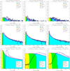 |
Fig. 4 Selected astrophysical dispersion histograms. The three columns show the histograms for G (left), GBP (center) and GRP (right) and the rows show different magnitude ranges: 3.5-5.4 (top), 10.0-10.5 (middle), and 16.5-17.0 (bottom). The GBP – GRP range is always 0.2−1.0 mag. Different colors are used to fill each astrophysical dispersion histogram to show the values of the variability flag for each filter (see text), note that there is one orange bin at most per panel. In addition, an empty histogram shows the corresponding total dispersion histogram. Finally, two lines of different color indicate the fitted function in the form of the astrophysical (pink) and total (purple) dispersions, respectively. The text at the top of each panel gives the results of the fits. |
2.4.2 On the use of the variability flag
We have already introduced the meaning of the variability flag. Figures 4 and 5 can be used to better interpret it. Depending on the G magnitude of the target, one band or another has a better sensitivity in terms of being able to measure its astrophysical dispersion. For the brightest stars GBP is the best band, for intermediate ones GRP is the option of choice, and for the faintest ones G is the preferred one. Taking as an example the magnitude and color ranges in Fig. 4, for G ~ 5 mag the three-sigma limit defined by the V flag is ~4 mmag for GBP, ~6 mmag for G, and ~7 mmag for GRP. Those values improve for G ~ 10 mag, with ~1.2 mmag for GRP, ~1.8 mmag for GBP, and ~2.5 mmag for G. When we go to fainter stars (G ~ 17 mag) the three-sigma limit becomes significantly higher: ~7 mmag for G, ~17 mmag for GRP, and ~23 mmag for GBP. Therefore, the best capabilities of Gaia for determining variability take place at intermediate magnitudes.
Which band is the best one for determining variability? In principle, there is information in all of them but, as we have just seen, the three sigma limit for GBP and GRP for faint stars (the majority of the sample) becomes significantly worse than the equivalent for G. Therefore, sG is the more uniform of the three bands and the first of the three letters in the variability flag is the one that is likely to be able to identify more variables. One can take the safe approach of considering only stars with a VVV flag as objects that are certainly variable but in doing so one would discard a relatively large number of faint objects with a VMM flag that have values of sX in the 10–20 mmag range in all three bands. On the other hand, one should be aware of the differences between G on the one hand and GBP and GRP on the other that appear in Fig. 2 that are propagated to Fig. 5. The sX,0 and sX distributions as a function of G for GBP and GRP are relatively smooth but those for G show discontinuities caused by the onboard data processing. Therefore, one should expect an increase in the number of discrepant sources arising from G due to this effect. Below we address this issue by analyzing the existence of outliers in the dispersion-dispersion planes, which adds information to the cases with variability flags where the three letters are not the same.
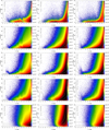 |
Fig. 5 Astrophysical photometric dispersions for G (left column), GBP (center column), and GRP (right column) for the five GBP – GRP ranges used in this work, from top to bottom: −1.0–0.2, 0.2−1.0, 1.0–1.5, 1.5–2.5, and 2.5–8.0 (in mag). The two lines in each plot mark the approximate boundaries between N and M flags (lower one) and between M and V flags (upper one). The horizontal axes are in mag and the vertical ones in mmag. |
2.4.3 Observed dispersion
A third question is whether the value of sX,0 determined from σX corresponds to the real photometric dispersion. The question is analyzed in the second paper of this series by comparing the values calculated here with those determined from the sample with light curves. In summary, the agreement is quite good but there are some details about which points are selected and which are rejected from the light curve and the calculation of final weighted mean magnitude by the Gaia team, as otherwise disagreements can appear in the G band. In Fig. 6 we show some examples of light curves built from Gaia EDR3 epoch photometry and the corresponding (independently obtained) values of sX,0 and sX.
2.4.4 Outliers in the dispersion-dispersion planes
A fourth question is the existence of outliers in the dispersiondispersion planes. In Fig. 7, we show the density diagrams for stars that are clearly variables in the three color combinations and in Figs. 8 and B.2 we show similar plots for the subsamples with R23 variability classifications but using as y axis the ratio of the previous y to x axes. Those figures are discussed below, as the structures seen in them are useful for the identification of different types of variable stars. Here we discuss structures of instrumental origin that appear in them. Comparing the left and center panels of the two bottom rows in Fig. 7, we see that in the left panels a region around (80 mmag, 10 mmag) is significantly more populated in the left panels compared to the center ones. In other words, there is an excess of sources with significantly larger  and
and  with respect to sG when comparing the global sample of this paper with the subsam-ple from R23. As no equivalent structure is seen in the top row, the phenomenon appears to affect
  and
and  simultaneously with respect to sG. We have verified this by selecting that the targets that simultaneously satisfy having the variability flag as VVV, sG < 20 mmag, log sG < log
  , and log sG < log
  are 5 060 097 and the ones that satisfy only the first three conditions are 5 327 967. As the first number is 95% of the second one, that indicates that the last condition introduces little extra restrictions on the selection and that the mentioned regions in the two panels share a large fraction of objects.
In addition to the difference in the previous paragraph between the whole sample and the R23 variables, two others are seen when comparing the left and center panels on Fig. 7. The first one is the extension towards low values of the dispersions (2–3 mmag) seen in the full sample and that is easily explained by the selection biases towards high dispersions in R23. The second one is an extension towards high values of sG (~50 mmag) that maintains low values of  or
or  (≲ 10 mmag) and that is symmetrical with respect to the diagonal with respect to the one in the previous paragraph but with fewer targets involved. In summary, there are targets that have anomalously high values of
  and
and  for a given sG and targets that have anomalously high values of sG for a given
  or
or  .
.
The likely explanation for those effects is given by Holl et al. (2023). In the presence of close companions or nebulosity, the photometric signal detected by Gaia in a given pass depends on the scan angle. In the case of equal-magnitude binaries observed in G (their Fig. 6), which are obtained by PSF fitting, the pair is always unresolved if the separation is less than 200 mas and always resolved if it is more than 400 mas. For the intermediate regime, the pair is resolved depending on the angle formed by the separation vector and the direction of the scan. As it is typical with binary detection using almost any technique, those separation limits become larger if there is a significant magnitude difference between the components (see e.g. Fig. 2 in Maíz Apellániz 2010 and Fig. 7 in Sana et al. 2014). Gbp and GRP observations, on the other hand, are obtained by aperture photometry with a rectangular box of 2."0 × 3."5 (their Fig. 11). In that case, the pair is resolved depending on the angle when the separation is at least 2–3". A working hypothesis is that the outliers in the dispersion-dispersion planes are caused mainly by visual binaries of different separations.
We have investigated this issue and discovered that many of the stars with anomalously large values of  and
and  indeed have companions ~2" away with a relatively small magnitude difference. This can be seen more clearly in the (better studied) bright subsample, as most of those objects have entries in the Washington Double Star catalog (WDS; Mason et al. 2001). With respect to the symmetrical case of high sG and low
  and #
and # , Vinagre Maqueda (2023) identified three systems (RX J0507.2+3731A, G 146–035, and 2MASS J21372900–0555082) with a bright companion separated by 200–500 mas, photometric dispersions in G much larger than in GBP and GRP, and light curves that supported those photometric dispersions. In addition, their ipd_gof_harmonic_amplitude and ipd_frac_multi_peak parameters (Holl et al. 2023) are anomalously high, supporting our idea. Therefore, the hypothesis above is likely to be correct but we cannot discard other effects. For example, stars close in G to one of the magnitudes used as a limit for the choice of electronic gates (e.g. G = 13 mag, see Fig. 2) could also experience spurious high values of sG. In any case, the safest approach for such outliers is to take the lowest dispersion of the three as the one closer to the real one.
Another way to look at this issue is with the average value of C* as a function of each pair of astrophysical dispersions (Fig. 9). There we see that most of the  plane has low averages values of C*, a sign of little contamination as a function of either band, with only very high values of either
  or
or  having high average values of C*. On the other hand, in the two plots where either
  or
or  is combined with sG, the regions occupied by the two types of outliers described above are seen as having high values of C*. Therefore, C* appears to be a good filter to detect cases with contaminated astrophysical dispersions.
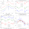 |
Fig. 6 Light curves for four of the targets with epoch photometry. Top left: AG Car, an LBV properly classified in R23. Top right: ALS 12 688, not given a classification type there but classified as an eclipsing binary in paper II of this series (Holgado et al., in prep.). Bottom left: HD 3885, classified as a slowly pulsating B star in R23 and as an α2 CVn variable in SIMBAD. Bottom right: OGLE LMC-CEP-101, classified as a Cepheid in that paper. The last three panels are phased with the best fitting period in each case (2.020 11 d, 1.815 67 d, and 8.190 73 d, respectively). The solid circles with error bars indicate the Gaia DR3 epoch measurements while the open circles with double error bars indicate the average magnitudes and the total and astrophysical dispersions determined in this paper (when both are similar the double error bars overlap). For OGLE LMC-CEP-101 the median magnitudes are subtracted in the vertical axis to allow for a higher dynamical range to be visualized. |
2.4.5 Validation summary
The provided astrophysical dispersions are overall a good description of reality but, as with all massive amounts of data, they have to be used with caution. Be aware of the limitations indicated by the variability flag and on the lookout for cases where one of the dispersions is very different from the other two, as in those cases it is likely that the higher value(s) are not real.
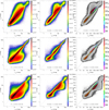 |
Fig. 7 Astrophysical dispersion-dispersion density diagrams for the three color combinations for stars that are classified as VVV here and have dispersion uncertainties |

3 Results
3.1 The dispersion-dispersion planes
We start by looking at the distribution of the sample in the dispersion-dispersion planes, which we already introduced in the previous section to mention the existence of outliers there caused by instrumental issues. The distribution is shown in Fig. 7 for the stars that are clearly variable, which we define as those classified as VVV and with dispersion uncertainties lower than 1 mmag in the three bands. The first column shows the density for all stars that satisfy those conditions and the second one the density for the subsample with R23 variability classifications. The third column is a gray-scale version of the second one with colors used to indicate the density distribution of eight of the most common types of variables, which together comprise almost 99% of all of the R23 sample analyzed here (see Table 1). In addition, in Fig. B.2 we show equivalent plots for each of the variable types in R23 but in this case plotting one astrophysical dispersion in the horizontal axis and the ratio of two in the vertical axis. Finally, Table 2 lists the properties extracted from Fig. B.2.
Figure 7 shows that the three dispersion-dispersion pairs are highly correlated, as expected since stars vary in similar ways in all optical bands to a first approximation. However, there is significant structure within each diagram. For the middle row (sG vs.  ), the correlation between the two dispersions is quite tight with the only exception of the instrumental effect described in the previous section caused by the different nature of the G and GRP photometry. For the other two rows where
  is involved the correlation is not as tight and at least three trends are seen: one close to the diagonal line (with
  slightly larger than
  or sG) that runs for most of the extension of the diagram, a second one with
  significantly larger than the other dispersion, and a third one in between the two that is seen only at large values of
  (200 to 300 mmag). The distinction between the three trends is seen in both the top and bottom rows but is more clear in the top one (
 vs.
vs.  ), as there is a better separation between the two passbands. The right column indicates that different trends correspond to different types of variables: the second trend is dominated by LPVs, the third one by RR Lyrae stars and Cepheids, and the first one by the other five types. In addition, different types have significantly different ranges in dispersion (with some biases that we discuss below). Therefore, our first result is that the location of the targets in the dispersion-dispersion planes, most notable on
  vs.
vs.  , can be used to constrain their variability type. This is a confirmation of what was found by Mowlavi et al. (2021) using Gaia DR2 data and a similar analysis as the one in this paper. The main additions here are: (a) the use of the superior quality DR3 data, (b) the subtraction of the instrumental component of the photometric dispersion, and (c) the inclusion of information from the R23 results.
Before proceeding further with the idea of using the location of the targets in the dispersion-dispersion planes to constrain their variability type, there are two types of biases that have to be considered. The first one is introduced by our criterion that only VVV objects with smaller than 1 mmag are considered. That criterion eliminates low-dispersion targets, especially faint ones. It can be determined from Table 2, where we list the percentage of stars of each type in the R23 sample that pass the criterion.
Types with high typical values of sX are little affected by the criterion, with R CrB stars, the one with the highest values, not having a single target excluded. The exception there are short timescale variables, microlensing events, and AGNs, for which many targets are excluded for being too faint. In general, low-dispersion variables such as solar-like and δ Sct+ stars have a large percentage excluded, indicating that their median values of sX in Table 2 are overestimated. The second type of bias is the selection criterion used by R23 to include stars in their sample. Such a bias is harder to determine but it is present, as seen by comparing the left and center columns in Fig. 7: the second trend mentioned above associated to LPV variables is continuous in the top and bottom panels of the first column but is interrupted around  mmag in their equivalents in the center column. This indicates that LPVs in the R23 sample are biased towards those with large amplitudes, an effect that is also seen in the lower rows of Fig. B.1. Therefore, both biases should be at work in Table 2 and one would expect that the values of sX should be smaller in general.
Looking into the specific variable-type categories in Table 2 and Fig. B.2, there are several interesting results:
Eclipsing binaries have values of nearly 1.0 in the three median dispersion ratios with little scatter. Ideal eclipsing binaries of identical effective temperature for each component should indeed have ratios of 1.0 and if the temperature difference is small they should not stray far away from that. Therefore, this result validates our technique and confirms what was found by Mowlavi et al. (2021) using Gaia DR2 data.
In general, the redder the target class, the larger
 becomes (Fig. 10). This is a expected behavior for intrinsically (not orbitally) variable stars, as in a cool star a small change in temperature has a larger flux effect in the blue than in the red, and in a hot star the effect is reversed. However, the correlation is not perfect due to the biases mentioned above, the presence of extinction confounding intrinsic and observed colors, and the existence of diverse origins and details for the variability of different types (right panel of Fig. 10). For example, M stars located near the ZAMS have significantly larger values of
  than those that have experienced some evolution.
This is consistent with young cool photospheres being more active at shorter wavelengths than older ones. A comparison of the right panel of Fig. 10 with the right panel of Fig. 23 of Mowlavi et al. (2021) shows the improvement from DR2 to DR3, as we are now able to sample the HRD better because of two effects: the better quality of DR3 and the fact that our procedure allows us to reach variables with smaller amplitudes (the sample in Mowlavi et al. 2021 contains only large-amplitude variables).
As a corollary of the previous point, the only two types with median
 lower than 1.0 are Be+ and α Cyg stars, which include most of the massive early-type stars analyzed by R23. They are not the ones with lower value of GBP – GRP in Table 2 due to their higher average extinction (despite the presence of many LMC+SMC stars among them, see below) but they are likely the two types with the lowest unreddened median values of Gbp – Grp.
Cepheids and RR Lyrae stars occupy a relatively distinct (but common for the two types) parameter space around sX of 100-200 mmag and
 around 1.6. That is the same value found by Mowlavi et al. (2021) using Gaia DR2 data.
Some types have complex distributions in Fig. B.2, a likely consequence of the fact that they are a mixture of different subtypes. For example, most of the δ Sct+ stars have values of sX lower than 10 mmag but two tails extend towards higher values with different
 : one around 1.0 and another around 1.3. LPVs have one major concentration around
  of 30–100 mmag and
  of 2.0–2.5 (truncated towards lower values of
  , see above), but with a tail extending towards much larger values of
  and with a distinct group around
  of 500–1000 mmag. The latter are likely highly variable AGB stars. Similar results were found by Mowlavi et al. (2021) using Gaia DR2 data.
The most variable type by far is that of R CrB stars. In addition to the already mentioned RR Lyr, Cepheid, and LPV types, two others that also have large values of sx are CVs and symbiotic stars.
Observed properties for different types of variables selecting stars classified as VVV and with dispersions uncertainties  lower than 1 mmag in the three bands.
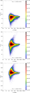 |
Fig. 8 Example of an astrophysical dispersion-dispersion ratio density diagram for the three color combinations for one variable type in R23 selecting stars that are classified as VVV here and have dispersions uncertainties lower than 1 mmag in the three bands. See Fig. B.2 for the whole set. |
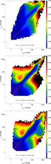 |
Fig. 9 Average C* as a function of the pairs of astrophysical dispersion for stars that are classified as VVV and have dispersion uncertainties lower than 1 mmag in the three bands (left column of Fig. 7). Only cells with at least 5 objects are plotted. |
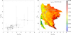 |
Fig. 10 Behavior of |


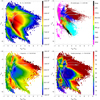 |
Fig. 11 Color-absolute magnitude style diagrams for the sample in this paper with accurate distances. Top left: source density. Top right: variable types from the R23 subsample with classifications. Bottom left: average G astrophysical dispersion. Bottom right: percentage of objects with VVV variability flag. Isochrones for 1 Ma, 10 Ma, 100 Ma, 1 Ga, and 10 Ga (in all cases for solar metallicity) are plotted in grey, with the isochrones being a combination of Geneva (Lejeune & Schaerer 2001) for high-mass stars and Padova (Girardi et al. 2000; Salasnich et al. 2000) for low-mass stars (see Maíz Apellániz 2013). The two black dotted vertical lines in the first panel show the location of the color limits for the calculation of the instrumental dispersion. The discontinuity seen around Gabs = −1.5 mag is caused by the inclusion of the LMC (and, to a lesser degree, the SMC at difference of half a magnitude) stars, which dominate the Gaia luminous star population if one does not correct for extinction (compare with Fig. 14). In the top right panel the number of plotted sources per variable type is capped at 10 000 to allow all types to be seen better. |
3.2 Color-absolute magnitude diagrams
In this subsection we analyze the behavior of Gaia photometric variability across the HR diagram. First, we select the sample of stars with  described above, which automatically excludes QSOs and a small number of luminous Local Group sources not in the LMC and SMC3. The sample of 105 576353 stars is subdivided into Galactic (MW), LMC, and SMC samples. The full sample and the three subsamples are shown in Figs. 11–14, respectively. Each of those figures has four panels: [a] a CAMD (CMD for the LMC and SMC) density plot, [b] the location of the R23 variables (capped at 10 000 stars per type and with the less numerous types grouped in an "other" category), [c] the average sG as a function of color of magnitude for all stars independent of the variability flag, and [d] the percentage of stars with a variability flag of VVV as a function of color and magnitude.
We provide four different figures because each shows different characteristics. The LMC and SMC subsamples have considerably less objects than the Galactic one and they only cover the brightest part of the Hertzsprung-Russell diagram (HRD), but they have two important advantages: their extinction is negligible compared to the Galaxy (hence allowing a straightforward comparison between the CAMD/CMD and the HRD) and the inclusion of two other galaxies allows for the analysis of potential metallicity effects. A comparison between Figs. 11 and 14 reveals that most stars in the full sample with Gabs brighter than −1.5 mag are in the Magellanic Clouds because most of the bright OB stars in the Milky Way have extinctions that move them downward and to the right in the CAMD4. Massive-star astronomers know well that OB stars (even those within a few kpc) are a needle in a Galactic haystack.
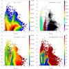 |
Fig. 12 Same as Fig. 11 but only for LMC targets, in the form of color-magnitude diagrams (m – M = 18.473 mag) and showing the isochrones for LMC metallicity for 1 Ma, 10 Ma, 32 Ma, 100 Ma, and 1 Ga. |
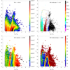 |
Fig. 13 Same as Fig. 11 but only for SMC targets, in the form of color-magnitude diagrams (m – M = 18.993 mag) and showing the isochrones for SMC metallicity for 1 Ma, 10 Ma, 32 Ma, 100 Ma, and 1 Ga. |
3.2.1 The LMC
We start discussing the LMC with Fig. 12. The CMD there is a version of the (top part of the) left panel of Fig. 2 in Luri et al. (2021), which we briefly summarize here. The two most obvious density concentrations are the nearly vertical one on the left (the hot-star MS) and the curved one on the left composed by RGB stars in its nearly vertical part and AGB stars in its nearly horizontal one (see Luri et al. 2021). In addition, there are other interesting structures that deserve attention:
The area termed BL (blue loop) by Luri et al. (2021) is encompassed by two overdensities that originate at GBP – GRP ~ 1.2 mag, G ~ 16.5 mag and extend towards the top. The two overdensities are the two extremes of the blue loop characteristic of 3–10 M⊙ stars, as seen in the 32 Ma and 100 Ma isochrones which indeed span the range between the two overdensities, small for 3 M⊙ stars and increasingly larger with mass. This agreement validates the Padova (100 Ma) and Geneva (32 Ma) isochrones employed. The right overdensity corresponds to the bright red giant (BRG, in luminosity class terms) but extends to the red supergiants (RSGs), as it includes stars above the 32 Ma isochrone5. The left overdensity starts also at a GBP – GRP color that corresponds to the K spectral type but moves towards earlier types as it increases in luminosity until it reaches the A supergiant region.
Crossing the BL region nearly vertically around GBP – GRP ~ 1.0 mag there is a band with large values of sG and a corresponding high percentage of VVV objects. The top right panel indicates that this band is populated mostly by Cepheids, with some RR Lyrae stars near the bottom (but note that Luri et al. 2021 put RR Lyrae stars at fainter magnitudes). The location of this instability strip does not correspond to a source overdensity except at its lower end around G ~ 16 mag. See below for a further analysis of the LMC instability strip. The near absence of differential extinction in the LMC with respect to the MW makes the instability strip significantly more clear than in the equivalent CAMDs for the MW (Fig. 14 here and Fig. 8 in Eyer et al. 2019).
A similar but less marked vertical structure is seen in the bottom panels of Fig. 12, with also larger values of sG and more VVV objects. In this case, it also appears to follow an overdensity, as the MS splits into a "blue branch" and a "red branch" at GBP – GRP ~ −0.2 mag and ~0.0 mag, respectively for G ~ 15 mag. The blue branch is the one with the lower values of sG and the red one the one with the higher values. The top right panel of Fig. 12 indicates that the variable stars in the red branch are classified in R23 as Be+ stars, dominated by Be stars but also including WRs, LBVs (or S Dor stars), and γ Cas stars. Given the location in the HRD, we suspect that most of these objects are indeed Be stars. The blue branch would then be dominated by normal (non-Be) MS stars.
To the right of the instability strip we find a region of low variability that indicates that 3–5 M⊙ stars are photometrically stable during their BRG phases. However, variability increases as we move towards higher luminosities and, especially, towards redder colors. The first trend (in luminosity) shows the largest gradient in the magnitude range of the evolved stars of the 32 Ma isochrone (G from 14 to 12.5 mag), which marks the transition from intermediate to massive stars. Therefore, RSGs are more variable than BRGs (but not extremely so in comparison with other luminous red stars) and that low mass stars are more variable during their AGB phase than in the immediately previous phases. Indeed, the highest values of sG are reached for the reddest stars in Fig. 12, that is, at the end of their AGB phase. The transition to higher values of sG takes place around GBP – GRP = 2.3 mag nearly independently of luminosity, pointing towards a temperature effect as extinction should be of little importance.
As we climb the MS following the non-Be (blue) branch we see an apparently contradictory phenomenon. The average sG remains approximately constant around 10–20 mmag but the percentage of VVV sources increases as we go from B to O stars. This is likely an instrumental effect, as for brighter stars it is easier to classify a target as VVV (Fig. 4).
There are few supergiants to the left of the instability strip, with those of B type appearing to be more variable than those of A and F type. This is likely related to the mass-loss bi-stability jump (Benaglía et al. 2007).
3.2.2 The SMC
Figure 13 shows the SMC equivalents to Fig. 12. Similar patterns are seen there but we point out some differences likely caused by metallicity effects.
The left overdensity of the blue loop is apparently missing. Instead, an overdensity is seen at lower luminosities and GBP – GRP ~ 0.5 mag. This could mean that the blue loop is present at SMC metallicities only for lower masses than for the LMC but we also have to consider that the SMC subsample has significantly less stars than the LMC one.
The separation between the blue (real) and red (Be) branches of the MS is more marked than for the LMC.
The transition to higher values of sG appears at a slightly lower value of GBP – GRP (~2.0 mag versus ~2.3 mag for the LMC) but AGB stars do not reach colors as red as in the LMC.
Similarly the BRGs and RSGs in the SMC are bluer for the same Gabs (Dorda et al. 2016).
3.2.3 The Milky Way
The Milky Way subsample is more than two orders of magnitude larger than those of the Magellanic Clouds combined and covers a much larger range in Gabs. At the same time, the Galactic Gaia CAMD is smeared by the effect of extinction, which moves stars downwards and to the right following curved trajectories (see e.g. Berlanas et al. 2023). As an example, the RC stars would all concentrate in a small region of the CAMD if it were not for extinction but in the upper left panel of Fig. 14 they are spread in a trajectory determined by extinction. In a forthcoming paper (Nogueras Lara et al., in prep.), we will analyze how extinction affects RC stars including non-linear photometric effects (Maíz Apellániz et al. 2020b) and differences in R5495 among sightlines (Maíz Apellániz et al. 2014; Maíz Apellániz & Barbâ 2018). A version of the lower panels of Fig. 14 using DR2 data is shown in Figs. 8 and 9 of Eyer et al. (2019).
To better analyze the different populations seen in Fig. 14, we divide the Galactic CAMD in six different regions: white dwarfs (WD), subdwarfs and cataclysmic variables (sd+CV), main sequence (MS), pre-main sequence (PMS), Cepheids and red clump (Cep+RC), and luminous red stars (LRS) according to the values given in Table 3 and shown in Fig. 15. The name of each region describes its dominant population(s) (with LRS objects encompassing RGBs, AGBs, BRGs, and RSGs) but other populations may be also present. For example, MS stars of different temperatures may be found in the PMS, Cep+RC, or LRS regions due to extinction. Below we analyze each of those six CAMD regions with the help of Figs. 14, 16, and 17 and Table 4. In the last two figures we plot for each region: (a) its sG histogram combining the information from Figs. 4 and B.1, (b) its  density diagram (to be compared with Fig. B.2), and (c) its
  density diagram (to be compared with the lower left plot of Fig. 14).
White dwarfs. This is the region less likely to be contaminated with sources that do not belong to the dominant population, as extinction can only move objects out but not in. The vast majority (99.6%) of the stars given a variable type by R23 receive the correct assignment as WD. White dwarfs have a high degree of variability in comparison to MS or RC stars (to be analyzed later on) with a nearly flat distribution for sG < 10 mmag and a power law with a slope of ~3.0 for sG > 10 mmag (top left panel of Fig. 16). Most of the sample consists of blue (young) WDs with GBP – GRP < 0.2, for which there is a relatively broad distribution in sG (top right panel of Fig. 16). The reddest (i.e. oldest) and less abundant WDs become progressively less variable starting at GBP – GRP ~ 0.2 (bottom left panel of Fig. 14 and upper right panel of Fig. 16). Eyer et al. (2019) did not mention this dependence of variability with color and age for WDs but it is hinted at in their Fig. 10, with the effect not as clear as in our DR3 results with the instrumental dispersion subtracted. R23 selected objects in this region with a bias for the most variable sources but not a strong one. Only a few hundred white dwarfs were previously known to be variable (Córsico 2020) and, to our knowledge, the flat distribution in sG (especially among young WDs) we see here was previously unknown.
Subdwarfs and cataclysmic variables. These two populations are clearly distinguished. sdBs have sG distributions very similar to that of (young) white dwarfs, with a flat distribution for sG < 10 mmag and a decline at higher values. Our sample includes ~8 times more stars than that of R23 but the two distributions are not too different. CVs, on the other hand, have much higher values of sG (reaching ~1 mag) and a narrow distribution of  around 1.0 or slightly higher. A minority of objects in this part of the
  plane are identified as eclipsing binaries. The majority of objects with sG larger than 30 mmag are likely to be CVs but are not identified as such in R23. This is the region with the highest fraction of targets with R23 variability classification (12.27%).
Main sequence. This is the region that includes the majority of the stars in the sample and, as a consequence, it contains a complex mixture of populations in terms of variables. Regarding the R23 sample, a little over half are solar-like (the most common type overall as well), whose distribution peaks around sG ~ 6 mmag. The second most abundant type, δ Sct+, follows a similar distribution with a slightly lower value of the peak in sG. Overall, the main-sequence region is dominated by low-variability stars, with a peak in the lower left panel of Fig. 16 around 1–2 mmag. The real peak could have an even lower value of sG, as such targets have large uncertainties and, hence, the distribution is not well constrained near zero. The third most common type of variables in R23, RS CVn, have typical values of sG around 20–30 mmag and of  around 1.3. Between sG of 3 mmag and 200 mmag the distribution can be approximated by a power law with α around 2.5 (with deviations associated to the different types of variables). At the high end the distribution has a cutoff and the population there is dominated by eclipsing binaries with a contribution from RR Lyr and a small one from YSOs and CVs at the extreme end. The double population of eclipsing binaries and RR Lyr at high values of sG is seen in the lower center panel of Fig. 16 as the two structures at
  and ~1.6, respectively.
Pre-main sequence. Contrary to the previous region, this one is heavily dominated by YSOs (91.2%) in the R23 population, with eclipsing binaries a distant second at 6.4%. The distribution in sG is very well fit by a power law with α = 2.75 that extends from 7 mmag to its high end. There are few objects with low variability in the pre-main sequence region in relative terms with other regions, as expected in a population dominated by YSOs. The high frequency of variable stars seen in the lower right panel of Fig. 14 was hinted at in Fig. 8 of Eyer et al. (2019), who only covered the boundary with the main-sequence region. A comparison between the total distribution and that of YSOs from R23 reveals their selection bias towards high values of sG, both in the slope and the cutoff of the distribution. Together with the white dwarfs region, they appear to be the two regions with the cleanest samples i.e. dominated by a single population.
Cepheids and red clump. This is a rather heterogeneous region defined by the (approximately vertical in the CAMD) Cepheid instability strip at zero extinction6 and by the (diagonal in the CAMD) red-clump extinction track, where the majority of the sample is actually located. Its most outstanding characteristic in terms of variability are its low values: the global distribution peaks around 1 mmag and only 0.59% of the targets have a variability class in R23. As this region is clearly dominated by RC stars (as shown by the density distribution in the CAMD), the conclusion is that those objects form one of the most stable categories among stellar types, another reason besides their well-defined magnitudes and color why they make excellent standard candles. This conclusion was already pointed out by Eyer et al. (2019). The variable minority is dominated by RS CVn stars (69.2% of R23 targets) but other populations are also present. At high values of sG there are also objects classified by R23 as eclipsing binaries, LPVs, YSOs, RR Lyr, and Cepheids.
Luminous red stars. This last region is occupied by luminous stars that appear as red, in most cases because they are intrinsically so (RGB, AGB, BRG, RSG) but in a few cases due to extinction, a phenomenon that significatively affects the majority of the sample. The luminous red stars and pre-main sequence regions are the two with the highest degrees of variability and in both cases they can be characterized by a power law that extends from sG ~ 7 mmag and a decline for sG ≲ 4 mmag. However, there are some differences in the distributions: the power-law fit here is not as good (there appears to be at least two subpopulations within the sample classified as LPVs by R23, something expected from what we saw for the Magellanic Clouds) and the measured α is lower (~2.2). The R23 sample is heavily dominated by LPVs (97.1%), which is actually a catch-all category for variable LRSs. R23 did a relatively complete job in catching the most variable sources: only three of the 40 targets with highest sG are missing in their list. Most of the stars with very high values of sG appear in the AGB catalog of Suh (2022).
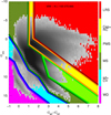 |
Fig. 15 Color-absolute magnitude source density diagram for the Milky Way subsample with the six different regions drawn. The gray scale uses the same values as the upper left panel of Fig. 14 and the background colors are applied only where no sources are found. |
Points used to define the limits for the six CAMD regions of the Milky Way subsample.
Number and percentage by R23 variable type for the six MW CAMD regions.
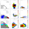 |
Fig. 16 Results for the first three of the six MW CAMD regions. Left column: astrophysical G dispersion histograms. The histograms have a uniform bin size but both the horizontal and vertical scales are logarithmic and the same for all plots to allow for better comparisons. The grey histogram shows the total sample and each panel also shows the histograms for the most common types of variable stars from the R23 data for that CAMD region (each in a different color that is maintained the same throughout this figure and the next for a given variable type) as well as another histogram with the rest of the R23 variables. The histograms built from R23 data are cumulative, so the top colored line represents all of the variables. The text at the top of each panel gives the number of stars and the percentage of stars with a variability classification from R23. The dotted diagonal line indicates the location of one star per bin to estimate Poisson fluctuations. Center column: astrophysical G dispersion-astrophysical GBP to GRP dispersion ratio density diagrams selecting stars that have uncertainties in the y axis lower than 50%. The number of selected stars and the total number are given at the top of each panel. The bin size is adjusted for each region depending on the number of sources. Right column: astrophysical G dispersion–GBP – GRP density diagrams. Note that the left and right columns include all stars in the regions while the center column only has a selection. |
 |
Fig. 18 G histograms for the stars in the LMC instability strip. The filled polygons are cumulative histograms for the full sample, non-RR Lyr non-Cepheid variables from R23, RR Lyr from R23, and Cepheids from R23. The blue unfilled line is an independent histogram containing all stars with sG > 17 mmag. |
4 Example applications
This paper is intended as a first step in the study of stellar variability using Gaia DR3 data. There is just too much information about different types of variables for a single paper. For that reason, here we just analyze three examples of what these results can be used for and leave further studies for future papers.
4.1 Cepheids in the LMC
As a first application, we analyze the objects in the instability strip in the LMC, which we define based on Fig. 12 as the region with:


The instability strip contains 35 956 stars from our sample, of which R23 classified 3947 (10.97%) as Cepheids, 75 (0.21%) as RR Lyr, and 181 (0.50%) as other types of variables. For the whole sample the median sG is 4.4 mmag but for the Cepheids it is 145.8 mmag (minimum of 17.4 mmag) and for the RR Lyr it is 191.0 mmag (minimum of 53.1 mmag). Therefore, the Cepheids and RR Lyr can be distinguished from other stars in principle from their photometric dispersions.
One use of the data in this paper is to search for LMC Cepheids not included in the R23 sample. We do that by selecting all stars in the instability strip with sG > 17 mmag (value selected from the minimum one for a Cepheid in the R23 LMC sample), computing its G-magnitude histogram, and comparing it with those of the different variable types (Fig. 18). We see there that R23 classified most of the stars in the LMC instability strip as Cepheids but that other variability types dominate at the brighter end and that RR Lyr start to make their appearance at the faintest end. A thorough search for Cepheids in the LMC would be the subject of a different paper but here we concentrate just on the brightest stars (G < 12.5 mag), which we list in Table 5, as a proof of concept. There we find 34 stars, of which:
Nine are classified as LPV by R23 so they are expected to be late-type stars. The four brightest have indeed SIMBAD spectral classifications of yellow or red supergiants. The next two have classifications of M0 without a luminosity class and of K2 III. Of the last three, one has no spectral classification but is listed as a long-period variable candidate, another one appears as a B8 Iab but has alternative classifications as a late-type object and an early+late binary, and the last one is listed as Be but has an alternative classification as C: using Gaia data.
Another nine are classified as Be+ by R23 so they are expected to be early-type stars. However, the six brightest appear in SIMBAD as yellow or red supergiants. Only the last three are classified as being of early type.
Another nine are classified as Cepheids by R23, of which six have spectral types in SIMBAD. All six appear as FGK giants or supergiants, as expected for Cepheids. The four objects with the highest values of sG among the list of 34 are listed as Cepheids by R23, indicating that high variability can be a discerning sign for them. Five of the nine have values of
 between 1.4 and 1.9 (that is close to the 1.6 value discussed above) but the other four have significantly higher ones.
The remaining seven are not in the R23 sample. Of those, the one that looks more promising as a Cepheid from our data is SV* HV 2827 in terms of its large value of sG and the closeness of its
 to 1.6. As it turns out, it is a known Cepheid (Martin & Warren 1979), thus showing that these data can find at least some Cepheids. We looked in the Gaia DR3 Cepheid catalog of Ripepi et al. (2023) but none of those seven stars are included.
Stars in the LMC instability strip with sG > 17 mmag and G < 12.5 mag.
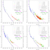 |
Fig. 19 Gaia EDR3 CAMDs/CMDs for four Villafranca clusters: Villafranca O-026 (σ Orionis cluster, top left), Villafranca O-016 (NGC 2264, top right), Villafranca O-021 (NGC 2362, bottom left), and Villafranca O-024 (γ Velorum cluster, bottom right) sorted from youngest to oldest. In each case we use the sample from Fig. 6 in Maíz Apellániz et al. (2022) with G ≤ 17 mag. The purple and green lines show MS isochrones with no extinction and with an average extinction appropriate to the cluster, respectively. Initial masses (in solar units) are labelled along the isochrones and the purple and green text at the right side of each panel gives the age and extinction parameters of the isochrones. The magenta line shows the extinguished PMS isochrone from Baraffe et al. (2015) of the age indicated by the text of the same color at the right side of the panel. The PMS isochrones reach up to 1.4 M⊙. |
4.2 PMS and MS stars in four Villafranca clusters
The Villafranca project (Maíz Apellániz et al. 2020a, 2022) is combining Gaia astrometry and photometry with data from ground-based spectroscopic (Maíz Apellániz et al. 2011, 2019) and photometric (Maíz Apellániz et al. 2021a) surveys to analyze Galactic stellar groups (clusters and subassociations) with massive stars. In Maíz Apellániz et al. (2022) we presented distances and memberships for 26 groups with O stars. Of those, we analyzed four low-foreground-extinction clusters in more detail and we selected the Gaia DR3 objects that have a high probability of membership. As a second application of the results in this paper, we cross-matched the stellar sample for those four clusters with the results here, discarding those objects fainter than G =17 mag or with six-parameter astrometric solutions. The resulting CAMDs/CMDs are plotted in Fig. 19, which is a new version of Fig. 1 in Maíz Apellániz et al. (2022) but now using a color code to place each target in one of four sG bins.
Results show a consistent pattern: a large majority of the stars that have already reached the MS are in the first sG bin (0–10 mmag) and most of the rest are in the second bin (10–30 mmag), with just one single object in the four clusters in the third bin (30–50 mmag). On the other hand, stars that are clearly in the PMS are concentrated in the last three bins, with only a few stars in the first bin. Furthermore, the fraction of objects in the third and fourth (sG > 50 mmag) bins is higher in the two youngest clusters (Villafranca O-026 and Villafranca O-016, PMS ages of ~2 Ma and ~4 Ma, respectively) than in the two oldest clusters (Villafranca O-021 and Villafranca O-024, PMS ages of ~5 Ma and ~8 Ma, respectively), indicating an age effect in the sense that variability decreases with age (see also Barber & Mann 2023).
As the four clusters have similar low extinctions and the transition from high to low variability appears to take place at a similar color (GBP – GRP ~ 0.8 mag), it is possible that the effective temperature of the stars is also playing a role, with hotter PMS stars being less variable than cooler ones. The competition between the two effects could be tested by analyzing massive PMS stars. However, we point out that the two stars with masses below 1 M⊙ in Villafranca O-016 and Villafranca O-021 that are closer to the MS isochrone (either because they are somewhat older or because they are cluster interlopers) have low values of sG, indicating that an age effect has to be present, in line with our comparison above between the MS and PMS regions. Therefore, the results in this paper can be used to characterize PMS populations in clusters.
4.3 The most variable stars in Gaia DR3
As a final application of these results, we list in Table 6 a total of 40 targets. Those are the ten targets each with the highest values of sG (a) overall, (b) without a variability classification in R23, (c) in then LMC, and (d) in the SMC.
The seven targets with the highest values of sG are all identified in R23 as R CrB variables, a rare kind of variable that has the highest average values in all three bands in Table 2 and whose members were individually checked by R23, discarding those that had lower probabilities despite being obviously variable. If we eliminate those, the highest-variability sample is dominated by LPVs. Both types are LRSs and the majority of cases are in the AGB phase. The ten stars with the highest values of sG are in the Milky Way but this is possibly a sample size effect (the LMC+SMC LRS samples are much smaller). LMC and SMC stars can also reach high values of sG but there are two significant differences between the Magellanic and Galactic samples in Table 6: (a) the first ones have extremely red colors (with the exception of one R CrB variable, the rest have all GBP – GRP > 3.5) while the second one is a mixed bag in GBP – GRP and (b) stars in the LMC and SMC have brighter Gabs (though extinction possibly plays a secondary role in that). As Magellanic interstellar extinction is generally low, this means that its highest variability sample is dominated by extreme AGB stars (see Figs. 12 and 13). The Galactic equivalent is more of a mixture.
R23 did a good job in selecting the targets with the highest variability but a significant number is not in their sample, including the second group of ten stars with sG larger than 1200 mmag in Table 6. The left column of Figs. 16 and 17 can be used to estimate the behavior in the different CAMD regions: for example, the LRS region appears to be more complete than the MS one. In particular we point out the case of R Hor (=HD 18 242), a relatively well-known Mira variable of sixth magnitude in G that is missing in the R23 sample. Most of that second group have red colors and are likely to be LPVs but some have GBP – GRP < 1 mag. One of those, HP Nor, is classified as a cataclysmic variable in SIMBAD. Therefore, the results in this paper can be used to select high-variability targets that are not included in R23.
5 Summary
In this paper we have presented the Gaia DR3 three-band photometric dispersions for the 145 million sources brighter than G = 17 mag, normal colors, and 5-parameter astrometric solutions. This work is intended to serve as a complement to R23: the information provided per star is smaller as we do not use epoch photometry but in exchange we use a much larger and unbiased sample. The results are made available so they can be used for future papers or for the preparation of DR4 by Gaia CU7.
Our main scientific results are:
A number of interesting results are observed for the Magellanic Clouds: the two regions in their CMDs with the highest variability are the Cepheid-RR Lyr instability strip and the coolest AGB stars, Be stars form a distinct branch with respect to the real main sequence in the CMD and show higher variability, the two ends of the blue loop are relatively quiet phases in terms of variability, and sG increases as we ascend in luminosity through the BRG-RSG branch without reaching the extreme values of the AGB stars.
Metallicity effects account for differences in some of the structures seen in the LMC and SMC CMDs, with a general displacement towards bluer colors for the position of red stars in the SMC with respect to the LMC, but the overall values of sG do not change much.
White dwarfs and B-type subdwarfs are significantly more variable than main-sequence stars. Most of the exceptions correspond to old WDs, indicating that the cause of the phenomenon becomes less important with age.
Main-sequence stars (and objects that fall in the same region of the CAMD) can show many types of variability but, overall, form one of the most stable regions in the HRD, with a peak in the sG distribution at just 1–2 mmag. This is an important consequence for astrobiology in terms of the stability of the habitable zone in short time scales.
We confirm that young stellar objects, on the other hand, are significantly more variable that MS stars in the optical in time scales of months, that is, what is sampled in Gaia DR3.
Red clump stars are also very stable, even more so than main-sequence stars. This is excellent news for their use as standard candles.
The LRS region of the Gaia CAMD is the most variable of all. The most variable objects are the extreme but uncommon R CrB variables and the more common AGB stars but other types of LRSs also contribute to the high variability.
There is a strong correlation between sG and position in the HRD in the four Villafranca clusters we have analyzed. Stars still in the PMS are significantly more variable than those that are already in the MS.
We plan to follow up this paper with others on variability using the results here. We think these results will be useful to the astronomical community for the analysis of DR3 data and for the preparation for DR4.
Sample stars with very high values of sG.
Acknowledgements
We thank Michael Weiler for the inspiration for this paper and useful comments and Sergio Simon-Diaz, Danny Lennon, Xavier Luri, Lee Patrick, and an anonymous referee for additional comments. J. M. A., G. H., and M. P. G. acknowledge support from the Spanish Government Ministerio de Ciencia e Innovación and Agencia Estatal de Investigación (10.13039/501 100 011033) through grant PGC2018-095 049-B-C22 and from the Consejo Superior de Investigaciones Científicas (CSIC) through grant 2022-AEP 005. J. A. C. acknowledges support from the Spanish Government Ministerio de Ciencia e Innovación and Agencia Estatal de Investigacion (10.13039/501 100011033) through grant PID2019-109522-GB-C51. This work has made use of data from the European Space Agency (ESA) mission Gaia (https://www.cosmos.esa.int/gaia), processed by the Gaia Data Processing and Analysis Consortium (DPAC, https://www.cosmos.esa.int/web/gaia/dpac/consortium). Funding for the DPAC has been provided by national institutions, in particular the institutions participating in the Gaia Multilateral Agreement. The Gaia data are processed with the computer resources at Mare Nostrum and the technical support provided by BSC-CNS. This research has made extensive use of the SIMBAD (http://simbad.u-strasbg.fr/simbad/) and VizieR (https://vizier.u-strasbg.fr/viz-bin/VizieR) databases, operated at CDS (https://cds.u-strasbg.fr), Strasbourg, France.
Appendix A Glossary
We provide a list of acronyms and terms used in this paper. In addition, acronyms for variable types are listed in Table 1.
α: (Modified) power-law slope, see Eqn. (2).
AGB: Asymptotic Giant Branch.
BRG: Bright Red Giant.
C*: Photometric contamination parameter from Eqn. (6) of Riello et al. (2021).
CAMD: Color–Absolute Magnitude Diagram.
CCD: Charged-Coupled Device.
CDS: Centre de Données astronomiques de Strasbourg.
CMD: Color–Magnitude Diagram.
CSIC: Consejo Superior de Investigaciones Cientificas.
CV: Cataclysmic Variable.
ESA: European Space Agency.
Gaia CU7: Gaia Coordination Unit 7 (Variability).
Gaia DPAC: Gaia Data Processing and AnalysisConsortium.
Gaia DR2: Second Gaia Data Release.
Gaia DR3: Third Gaia Data Release.
Gaia DR4: Fourth Gaia Data Release.
HRD: Hertzsprung-Russell Diagram.
LMC: Large Magellanic Cloud.
LRS: Luminous Red Star.
MS: Main Sequence.
MW: Milky Way.
PMS: Pre-main sequence.
QSO: Quasi-Stellar Object.
R23: Rimoldini et al. (2023).
RC: Red Clump.
RGB: Red Giant Branch.
RSG: Red SuperGiant.
sd(B): (B-type) sub dwarf.
SMC: Small Magellanic Cloud.
sX,0: Observed dispersion for band X (G, GBP, or GRP).
sX: Astrophysical dispersion for band X (G, GBP, or GRP), see Eqn. (1).
sX,c: Characteristic dispersion for band X (G, GBP, or GRP), see Eqn. (2).
sX,ins: Instrumental dispersion for band X (G, GBP, or GRP), modelled by a Gaussian of average sX,i and width σX,i
 : Astrophysical dispersion uncertainty for band X (G, GBP, or GRP).
WD: White Dwarf.
WDS: Washington Double Star catalog.
YSO: Young Stellar Object.
Appendix B Additional tables and figures
Fit results for the observed dispersions of G.
Fit results for the observed dispersions of GBP.
Fit results for the observed dispersions of GRP.
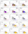 |
Fig. B.1 Total dispersion histograms used to calculate the instrumental dispersion as a function of magnitude and color. Each page shows the 15 plots for a given G magnitude range, starting with 3.0–5.3 mag. The three columns show the histograms for G (left), GBP (center) and GRP (right). The five rows show the GBP – GRP ranges, from top to bottom: −1.0–0.2, 0.2–1.0, 1.0–1.5, 1.5–2.5, and 2.5–8.0 (in mag). The histograms have a uniform bin size in logarithmic units (see the text for the bins used for fitting) and both the horizontal and vertical scales are logarithmic and the same in all plots to allow for better comparisons. The dotted diagonal line indicates the location of one star per bin to estimate Poisson fluctuations. |
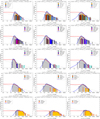 |
Fig. B.1 (continued from previous page). The grey histogram shows the total sample and each panel also shows the histograms for the three most common types of variable stars from the R23 data for that magnitude and color ranges (each in a different color that is maintained the same throughout the figure for a given variable type) as well as a fourth histogram with the rest of the R23 variables. The four histograms built from R23 data are cumulative, so the top colored line represents all of the variables. The blue line shows the fit for the total dispersion and the red line the corresponding distribution for the astrophysical (intrinsic) dispersion. The text at the top of each panel gives the results of the fits and the percentage of stars with a variability classification from R23. |
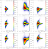 |
Fig. B.2 Astrophysical dispersion–dispersion ratio density diagrams for the three color combinations for each of the variable types in R23 selecting stars that are classified as VVV here and have dispersions uncertainties σSX lower than 1 mmag in the three bands. Each column shows a different variable type sorted as in Table 1 and each row a different color combination. The bin size is adjusted for each variable type depending on the number of sources. |
References
- Andrew, S., Swihart, S. J., & Strader, J. 2021, ApJ, 908, 180 [NASA ADS] [CrossRef] [Google Scholar]
- Baraffe, I., Homeier, D., Allard, F., & Chabrier, G. 2015, A&A, 577, A42 [NASA ADS] [CrossRef] [EDP Sciences] [Google Scholar]
- Barber, M. G., & Mann, A. W. 2023, ApJ, 953, 127 [NASA ADS] [CrossRef] [Google Scholar]
- Barlow, B. N., Corcoran, K. A., Parker, I. M., et al. 2022, ApJ, 928, 20 [NASA ADS] [CrossRef] [Google Scholar]
- Belokurov, V., Erkal, D., Deason, A. J., et al. 2017, MNRAS, 466, 4711 [Google Scholar]
- Benaglía, P., Vink, J. S., Martí, J., et al. 2007, A&A, 467, 1265 [NASA ADS] [CrossRef] [EDP Sciences] [Google Scholar]
- Berlanas, S. R., Maíz Apellániz, J., Herrero, A., et al. 2023, A&A, 671, A20 [NASA ADS] [CrossRef] [EDP Sciences] [Google Scholar]
- Carrasco, J. M., Evans, D. W., Montegriffo, P., et al. 2016, A&A, 595, A7 [NASA ADS] [CrossRef] [EDP Sciences] [Google Scholar]
- Cioni, M. R. L., van der Marel, R. P., Loup, C., & Habing, H. J. 2000, A&A, 359, 601 [Google Scholar]
- Córsico, A. H. 2020, IAUS, 357, 93 [Google Scholar]
- Deason, A. J., Belokurov, V., Erkal, D., Koposov, S. E., & Mackey, D. 2017, MNRAS, 467, 2636 [NASA ADS] [CrossRef] [Google Scholar]
- Dorda, R., Negueruela, I., González-Fernández, C., & Tabernero, H. M. 2016, A&A, 592, A16 [NASA ADS] [CrossRef] [EDP Sciences] [Google Scholar]
- Eyer, L., Rimoldini, L., Audard, M., et al. 2019, A&A, 623, A110 [NASA ADS] [CrossRef] [EDP Sciences] [Google Scholar]
- Eyer, L., Audard, M., Holl, B., et al. 2023, A&A, 674, A13 [NASA ADS] [CrossRef] [EDP Sciences] [Google Scholar]
- Girardi, L., Bressan, A., Bertelli, G., & Chiosi, C. 2000, A&AS, 141, 371 [NASA ADS] [CrossRef] [EDP Sciences] [Google Scholar]
- Guidry, J. A., Vanderbosch, Z. P., Hermes, J. J., et al. 2021, ApJ, 912, 125 [NASA ADS] [CrossRef] [Google Scholar]
- Holl, B., Fabricius, C., Portell, J., et al. 2023, A&A, 674, A25 [NASA ADS] [CrossRef] [EDP Sciences] [Google Scholar]
- Iorio, G., Belokurov, V., Erkal, D., et al. 2018, MNRAS, 474, 2142 [NASA ADS] [CrossRef] [Google Scholar]
- Jiménez-Arranz, Ó., Romero-Gómez, M., Luri, X., & Masana, E. 2023a, A&A, 672, A65 [NASA ADS] [CrossRef] [EDP Sciences] [Google Scholar]
- Jiménez-Arranz, Ó., Romero-Gómez, M., Luri, X., et al. 2023b, A&A, 669, A91 [NASA ADS] [CrossRef] [EDP Sciences] [Google Scholar]
- Lejeune, T., & Schaerer, D. 2001, A&A, 366, 538 [NASA ADS] [CrossRef] [EDP Sciences] [Google Scholar]
- Lindegren, L., Klioner, S. A., Hernández, J., et al. 2021a, A&A, 649, A2 [EDP Sciences] [Google Scholar]
- Lindegren, L., Bastian, U., Biermann, M., et al. 2021b, A&A, 649, A4 [EDP Sciences] [Google Scholar]
- Luri, X., Brown, A. G. A., Sarro, L. M., et al. 2018, A&A, 616, A9 [NASA ADS] [CrossRef] [EDP Sciences] [Google Scholar]
- Luri, X., Chemin, L., Clementini, G., et al. 2021, A&A, 649, A7 [NASA ADS] [CrossRef] [EDP Sciences] [Google Scholar]
- Maíz Apellániz, J. 2001, AJ, 121, 2737 [Google Scholar]
- Maíz Apellániz, J. 2005, in ESA SP, 576, The Three-Dimensional Universe with Gaia, eds. C. Turon, K. S. O’Flaherty, & M. A. C. Perryman, 179 [Google Scholar]
- Maíz Apellániz, J. 2010, A&A, 518, A1 [NASA ADS] [CrossRef] [EDP Sciences] [Google Scholar]
- Maíz Apellániz, J. 2013, in HSA 7, 657 [Google Scholar]
- Maíz Apellániz, J. 2022, A&A, 657, A130 [NASA ADS] [CrossRef] [EDP Sciences] [Google Scholar]
- Maíz Apellániz, J., & Barbâ, R. H. 2018, A&A, 613, A9 [CrossRef] [EDP Sciences] [Google Scholar]
- Maíz Apellániz, J., & Ubeda, L. 2005, ApJ, 629, 873 [CrossRef] [Google Scholar]
- Maíz Apellániz, J., & Weiler, M. 2018, A&A, 619, A180 [Google Scholar]
- Maíz Apellániz, J., Sota, A., Walborn, N. R., et al. 2011, in HSA 6, 467 [Google Scholar]
- Maíz Apellániz, J., Evans, C. J., Barbâ, R. H., et al. 2014, A&A, 564, A63 [NASA ADS] [CrossRef] [EDP Sciences] [Google Scholar]
- Maíz Apellániz, J., Sota, A., Arias, J. I., et al. 2016, ApJS, 224, 4 [CrossRef] [Google Scholar]
- Maíz Apellániz, J., Trigueros Páez, E., Jiménez Martínez, I., et al. 2019, in HSA 10, 420 [Google Scholar]
- Maíz Apellániz, J., Crespo Bellido, P., Barbá, R. H., Fernández Aranda, R., & Sota, A. 2020a, A&A, 643, A138 [NASA ADS] [CrossRef] [EDP Sciences] [Google Scholar]
- Maíz Apellániz, J., Pantaleoni González, M., Barbá, R. H., García-Lario, P., & Nogueras-Lara, F. 2020b, MNRAS, 496, 4951 [Google Scholar]
- Maíz Apellániz, J., Alfaro, E. J., Barbá, R. H., et al. 2021a, MNRAS, 506, 3138 [CrossRef] [Google Scholar]
- Maíz Apellániz, J., Pantaleoni González, M., & Barbá, R. H. 2021b, A&A, 649, A13 [NASA ADS] [CrossRef] [EDP Sciences] [Google Scholar]
- Maíz Apellániz, J., Barbá, R. H., Fernández Aranda, R., et al. 2022, A&A, 657, A131 [NASA ADS] [CrossRef] [EDP Sciences] [Google Scholar]
- Martin, W. L., & Warren, P. R. 1979, South Afr. Astron. Observ. Circ., 1, 98 [Google Scholar]
- Mason, B. D., Wycoff, G. L., Hartkopf, W. I., Douglass, G. G., & Worley, C. E. 2001, AJ, 122, 3466 [Google Scholar]
- Mowlavi, N., Rimoldini, L., Evans, D. W., et al. 2021, A&A, 648, A44 [EDP Sciences] [Google Scholar]
- Mowlavi, N., Holl, B., Lecoeur-Taïbi, I., et al. 2023, A&A, 674, A16 [NASA ADS] [CrossRef] [EDP Sciences] [Google Scholar]
- Pietrzyński, G., Graczyk, D., Gallenne, A., et al. 2019, Nature, 567, 200 [Google Scholar]
- Prusti, T., de Bruijne, J. H. J., Brown, A. G. A., et al. 2016, A&A, 595, A1 [NASA ADS] [CrossRef] [EDP Sciences] [Google Scholar]
- Riello, M., De Angeli, F., Evans, D. W., et al. 2021, A&A, 649, A3 [NASA ADS] [CrossRef] [EDP Sciences] [Google Scholar]
- Rimoldini, L., Holl, B., Gavras, P., et al. 2023, A&A, 674, A14 [NASA ADS] [CrossRef] [EDP Sciences] [Google Scholar]
- Ripepi, V., Clementini, G., Molinaro, R., et al. 2023, A&A, 674, A17 [NASA ADS] [CrossRef] [EDP Sciences] [Google Scholar]
- Salasnich, B., Girardi, L., Weiss, A., & Chiosi, C. 2000, A&A, 361, 1023 [NASA ADS] [Google Scholar]
- Sana, H., Le Bouquin, J.-B., Lacour, S., et al. 2014, ApJS, 215, 15 [Google Scholar]
- Suh, K.-W. 2022, J. Korean Astron. Soc., 55, 195 [NASA ADS] [Google Scholar]
- Vallenari, A., Brown, A. G. A., Prusti, T., et al. 2023, A&A, 674, A1 [NASA ADS] [CrossRef] [EDP Sciences] [Google Scholar]
- Vinagre Maqueda, A. R. 2023, Master’s thesis, CARMENES target characterization: Carmencita and Gaia, Universidad Complutense de Madrid, Spain [Google Scholar]
- Vioque, M., Oudmaijer, R. D., Schreiner, M., et al. 2020, A&A, 638, A21 [NASA ADS] [CrossRef] [EDP Sciences] [Google Scholar]
Subsequent to Luri et al. (2021), Jiménez-Arranz et al. (2023a,b) have produced new membership lists for the LMC and SMC, but for stars within 10° of the respective galactic centers and with G ≤ 17 mag the differences are minor.
We remind the reader that for the Magellanic Clouds we are using the Pietrzyński et al. (2019) and Cioni et al. (2000) values for the distances, which satisfy the equivalent to  .
.
There is confusion in the literature about the nomenclature for luminous red stars, with a mix based on luminosity classes (supergiants or I, bright giants or II, and giants or III) and on evolutionary phases (RGB, RC, AGB, and RSG). Here we call BRGs the stars in the same branch in the LMC CMD as RSGs (massive stars) but below them i.e. of intermediate mass, independently of whether they are in that region on their first pass (before the blue loop) or the second one (after the blue loop).
All Tables
Observed properties for different types of variables selecting stars classified as VVV and with dispersions uncertainties lower than 1 mmag in the three bands.
Points used to define the limits for the six CAMD regions of the Milky Way subsample.
All Figures
|
Fig. 1 Source density (logarithmic scale) in the color-magnitude plane for the sample in this paper. Dotted black lines indicate the magnitude-color bins used to determine the characteristics of the photometric dispersion. |
| In the text | |
|
Fig. 2 Observed photometric dispersions for G (left column), GBP (center column), and GRP (right column) for the five GBP – GRP ranges used in this work, from top to bottom: −1.0–0.2, 0.2−1.0, 1.0–1.5, 1.5–2.5, and 2.5–8.0 (in mag). The plotted points and error bars are the measurements of the instrumental dispersions sX,i and their widths σX,i for each magnitude bin and the grey line joining them is a cubic spline fit. The horizontal axes are in mag and the vertical ones in mmag. |
| In the text | |
|
Fig. 3 Example of a total dispersion histogram used to calculate the instrumental dispersion as a function of magnitude and color (see Fig. B.1 for the whole set). The histogram has a uniform bin size in logarithmic units (see the text for the bins used for fitting) and both the horizontal and vertical scales are logarithmic. The dotted diagonal line indicates the location of one star per bin to estimate Poisson fluctuations. The light grey histogram shows the total sample, the color histograms the three most common types of variable stars from the R23 data for that magnitude and color ranges, and the dark grey histogram the rest of the R23 variables. The four histograms built from R23 data are cumulative, so the top colored line represents all of the variables. The blue line shows the fit for the total dispersion and the red line the corresponding distribution for the astrophysical (intrinsic) dispersion. The text at the top gives the results of the fits and the percentage of stars with a variability classification from R23. |
| In the text | |
|
Fig. 4 Selected astrophysical dispersion histograms. The three columns show the histograms for G (left), GBP (center) and GRP (right) and the rows show different magnitude ranges: 3.5-5.4 (top), 10.0-10.5 (middle), and 16.5-17.0 (bottom). The GBP – GRP range is always 0.2−1.0 mag. Different colors are used to fill each astrophysical dispersion histogram to show the values of the variability flag for each filter (see text), note that there is one orange bin at most per panel. In addition, an empty histogram shows the corresponding total dispersion histogram. Finally, two lines of different color indicate the fitted function in the form of the astrophysical (pink) and total (purple) dispersions, respectively. The text at the top of each panel gives the results of the fits. |
| In the text | |
|
Fig. 5 Astrophysical photometric dispersions for G (left column), GBP (center column), and GRP (right column) for the five GBP – GRP ranges used in this work, from top to bottom: −1.0–0.2, 0.2−1.0, 1.0–1.5, 1.5–2.5, and 2.5–8.0 (in mag). The two lines in each plot mark the approximate boundaries between N and M flags (lower one) and between M and V flags (upper one). The horizontal axes are in mag and the vertical ones in mmag. |
| In the text | |
|
Fig. 6 Light curves for four of the targets with epoch photometry. Top left: AG Car, an LBV properly classified in R23. Top right: ALS 12 688, not given a classification type there but classified as an eclipsing binary in paper II of this series (Holgado et al., in prep.). Bottom left: HD 3885, classified as a slowly pulsating B star in R23 and as an α2 CVn variable in SIMBAD. Bottom right: OGLE LMC-CEP-101, classified as a Cepheid in that paper. The last three panels are phased with the best fitting period in each case (2.020 11 d, 1.815 67 d, and 8.190 73 d, respectively). The solid circles with error bars indicate the Gaia DR3 epoch measurements while the open circles with double error bars indicate the average magnitudes and the total and astrophysical dispersions determined in this paper (when both are similar the double error bars overlap). For OGLE LMC-CEP-101 the median magnitudes are subtracted in the vertical axis to allow for a higher dynamical range to be visualized. |
| In the text | |
|
Fig. 7 Astrophysical dispersion-dispersion density diagrams for the three color combinations for stars that are classified as VVV here and have dispersion uncertainties |
| In the text | |
|
Fig. 8 Example of an astrophysical dispersion-dispersion ratio density diagram for the three color combinations for one variable type in R23 selecting stars that are classified as VVV here and have dispersions uncertainties lower than 1 mmag in the three bands. See Fig. B.2 for the whole set. |
| In the text | |
|
Fig. 9 Average C* as a function of the pairs of astrophysical dispersion for stars that are classified as VVV and have dispersion uncertainties lower than 1 mmag in the three bands (left column of Fig. 7). Only cells with at least 5 objects are plotted. |
| In the text | |
|
Fig. 10 Behavior of |
| In the text | |
|
Fig. 11 Color-absolute magnitude style diagrams for the sample in this paper with accurate distances. Top left: source density. Top right: variable types from the R23 subsample with classifications. Bottom left: average G astrophysical dispersion. Bottom right: percentage of objects with VVV variability flag. Isochrones for 1 Ma, 10 Ma, 100 Ma, 1 Ga, and 10 Ga (in all cases for solar metallicity) are plotted in grey, with the isochrones being a combination of Geneva (Lejeune & Schaerer 2001) for high-mass stars and Padova (Girardi et al. 2000; Salasnich et al. 2000) for low-mass stars (see Maíz Apellániz 2013). The two black dotted vertical lines in the first panel show the location of the color limits for the calculation of the instrumental dispersion. The discontinuity seen around Gabs = −1.5 mag is caused by the inclusion of the LMC (and, to a lesser degree, the SMC at difference of half a magnitude) stars, which dominate the Gaia luminous star population if one does not correct for extinction (compare with Fig. 14). In the top right panel the number of plotted sources per variable type is capped at 10 000 to allow all types to be seen better. |
| In the text | |
|
Fig. 12 Same as Fig. 11 but only for LMC targets, in the form of color-magnitude diagrams (m – M = 18.473 mag) and showing the isochrones for LMC metallicity for 1 Ma, 10 Ma, 32 Ma, 100 Ma, and 1 Ga. |
| In the text | |
|
Fig. 13 Same as Fig. 11 but only for SMC targets, in the form of color-magnitude diagrams (m – M = 18.993 mag) and showing the isochrones for SMC metallicity for 1 Ma, 10 Ma, 32 Ma, 100 Ma, and 1 Ga. |
| In the text | |
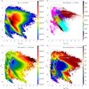 |
Fig. 14 Same as Fig. 11 but the MW subsample, i.e. excluding targets in the LMC and SMC. |
| In the text | |
|
Fig. 15 Color-absolute magnitude source density diagram for the Milky Way subsample with the six different regions drawn. The gray scale uses the same values as the upper left panel of Fig. 14 and the background colors are applied only where no sources are found. |
| In the text | |
|
Fig. 16 Results for the first three of the six MW CAMD regions. Left column: astrophysical G dispersion histograms. The histograms have a uniform bin size but both the horizontal and vertical scales are logarithmic and the same for all plots to allow for better comparisons. The grey histogram shows the total sample and each panel also shows the histograms for the most common types of variable stars from the R23 data for that CAMD region (each in a different color that is maintained the same throughout this figure and the next for a given variable type) as well as another histogram with the rest of the R23 variables. The histograms built from R23 data are cumulative, so the top colored line represents all of the variables. The text at the top of each panel gives the number of stars and the percentage of stars with a variability classification from R23. The dotted diagonal line indicates the location of one star per bin to estimate Poisson fluctuations. Center column: astrophysical G dispersion-astrophysical GBP to GRP dispersion ratio density diagrams selecting stars that have uncertainties in the y axis lower than 50%. The number of selected stars and the total number are given at the top of each panel. The bin size is adjusted for each region depending on the number of sources. Right column: astrophysical G dispersion–GBP – GRP density diagrams. Note that the left and right columns include all stars in the regions while the center column only has a selection. |
| In the text | |
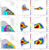 |
Fig. 17 Same as Fig. 16 for the last three of the six MW regions. |
| In the text | |
|
Fig. 18 G histograms for the stars in the LMC instability strip. The filled polygons are cumulative histograms for the full sample, non-RR Lyr non-Cepheid variables from R23, RR Lyr from R23, and Cepheids from R23. The blue unfilled line is an independent histogram containing all stars with sG > 17 mmag. |
| In the text | |
|
Fig. 19 Gaia EDR3 CAMDs/CMDs for four Villafranca clusters: Villafranca O-026 (σ Orionis cluster, top left), Villafranca O-016 (NGC 2264, top right), Villafranca O-021 (NGC 2362, bottom left), and Villafranca O-024 (γ Velorum cluster, bottom right) sorted from youngest to oldest. In each case we use the sample from Fig. 6 in Maíz Apellániz et al. (2022) with G ≤ 17 mag. The purple and green lines show MS isochrones with no extinction and with an average extinction appropriate to the cluster, respectively. Initial masses (in solar units) are labelled along the isochrones and the purple and green text at the right side of each panel gives the age and extinction parameters of the isochrones. The magenta line shows the extinguished PMS isochrone from Baraffe et al. (2015) of the age indicated by the text of the same color at the right side of the panel. The PMS isochrones reach up to 1.4 M⊙. |
| In the text | |
|
Fig. B.1 Total dispersion histograms used to calculate the instrumental dispersion as a function of magnitude and color. Each page shows the 15 plots for a given G magnitude range, starting with 3.0–5.3 mag. The three columns show the histograms for G (left), GBP (center) and GRP (right). The five rows show the GBP – GRP ranges, from top to bottom: −1.0–0.2, 0.2–1.0, 1.0–1.5, 1.5–2.5, and 2.5–8.0 (in mag). The histograms have a uniform bin size in logarithmic units (see the text for the bins used for fitting) and both the horizontal and vertical scales are logarithmic and the same in all plots to allow for better comparisons. The dotted diagonal line indicates the location of one star per bin to estimate Poisson fluctuations. |
| In the text | |
|
Fig. B.1 (continued from previous page). The grey histogram shows the total sample and each panel also shows the histograms for the three most common types of variable stars from the R23 data for that magnitude and color ranges (each in a different color that is maintained the same throughout the figure for a given variable type) as well as a fourth histogram with the rest of the R23 variables. The four histograms built from R23 data are cumulative, so the top colored line represents all of the variables. The blue line shows the fit for the total dispersion and the red line the corresponding distribution for the astrophysical (intrinsic) dispersion. The text at the top of each panel gives the results of the fits and the percentage of stars with a variability classification from R23. |
| In the text | |
|
Fig. B.2 Astrophysical dispersion–dispersion ratio density diagrams for the three color combinations for each of the variable types in R23 selecting stars that are classified as VVV here and have dispersions uncertainties σSX lower than 1 mmag in the three bands. Each column shows a different variable type sorted as in Table 1 and each row a different color combination. The bin size is adjusted for each variable type depending on the number of sources. |
| In the text | |
Current usage metrics show cumulative count of Article Views (full-text article views including HTML views, PDF and ePub downloads, according to the available data) and Abstracts Views on Vision4Press platform.
Data correspond to usage on the plateform after 2015. The current usage metrics is available 48-96 hours after online publication and is updated daily on week days.
Initial download of the metrics may take a while.