| Issue |
A&A
Volume 676, August 2023
|
|
|---|---|---|
| Article Number | A52 | |
| Number of page(s) | 30 | |
| Section | Planets and planetary systems | |
| DOI | https://doi.org/10.1051/0004-6361/202244850 | |
| Published online | 07 August 2023 | |
Revisiting equilibrium condensation and rocky planet compositions
Introducing the ECCOPLANETS code
1
Institut für Astrophysik und Geophysik, Georg-August-Universität Göttingen,
Friedrich-Hund-Platz 1,
37077
Göttingen, Germany
e-mail: t.timmermann@stud.uni-goettingen.de
2
Geowissenschaftliches Zentrum Abteilung Geochemie und Isotopengeologie,
Goldschmidtstraße 1,
37077
Göttingen, Germany
3
Centre for Earth Evolution and Dynamics, University of Oslo,
Sem Salands vei 2A ZEB-bygget
0371
Oslo, Norway
Received:
31
August
2022
Accepted:
13
June
2023
Context. The bulk composition of exoplanets cannot yet be directly observed. Equilibrium condensation simulations help us better understand the composition of the planets’ building blocks and their relation to the composition of their host star.
Aims. We introduce ECCOPLANETS, an open-source Python code that simulates condensation in the protoplanetary disk. Our aim is to analyse how well a simplistic model can reproduce the main characteristics of rocky planet formation. For this purpose, we revisited condensation temperatures (Tc) as a means to study disk chemistry, and explored their sensitivity to variations in pressure (p) and elemental abundance pattern. We also examined the bulk compositions of rocky planets around chemically diverse stars.
Methods. Our T-p-dependent chemical equilibrium model is based on a Gibbs free energy minimisation. We derived condensation temperatures for Solar System parameters with a simulation limited to the most common chemical species. We assessed their change (∆Tc) as a result of p-variation between 10−6 and 0.1 bar. To analyse the influence of the abundance pattern, key element ratios were varied, and the results were validated using solar neighbourhood stars. To derive the bulk compositions of planets, we explored three different planetary feeding-zone (FZ) models and compared their output to an external n-body simulation.
Results. Our model reproduces the external results well in all tests. For common planet-building elements, we derive a Tc that is within ±5 K of literature values, taking a wider spectrum of components into account. The Tc is sensitive to variations in p and the abundance pattern. For most elements, it rises with p and metallicity. The tested pressure range (10−6 − 0.1 bar) corresponds to ∆Tc ≈ +350 K, and for −0.3 ≤ [M/H] ≤ 0.4 we find ∆Tc ≈ +100 K. An increase in C/O from 0.1 to 0.7 results in a decrease of ∆Tc ≈ −100 K. Other element ratios are less influential. Dynamic planetary accretion can be emulated well with any FZ model. Their width can be adapted to reproduce gradual changes in planetary composition.
Key words: planets and satellites: composition / planets and satellites: formation / protoplanetary disks
© The Authors 2023
 Open Access article, published by EDP Sciences, under the terms of the Creative Commons Attribution License (https://creativecommons.org/licenses/by/4.0), which permits unrestricted use, distribution, and reproduction in any medium, provided the original work is properly cited.
This article is published in open access under the Subscribe to Open model. Subscribe to A&A to support open access publication.
1 Introduction
The chemical composition of rocky planets is, among other factors such as the surface temperature or the presence of a magnetic field, an important parameter with respect to the habitability and the potential existence of extraterrestrial life. The bulk composition of a planet can be roughly estimated using density measurements from observational data of radial velocity (planet mass) and planetary transits (planet radius; Fulton & Petigura 2018; Zeng et al. 2019; Fridlund et al. 2020; Otegi et al. 2020a,b; Schulze et al. 2021). Transit spectroscopy is beginning to provide answers regarding the existence of specific molecules in planetary atmospheres (Seager & Sasselov 2000; Brown 2001; Madhusudhan 2019; Brogi & Line 2019; Madhusudhan et al. 2021; Rustamkulov et al. 2022). However, the observational answer to the pivotal question of the composition of rocky planets, in particular the makeup of their interior structure, still remains largely elusive. Currently, the only technique that allows glimpses into solids compositions is the spectroscopic analysis of polluted white dwarfs (Jura & Young 2014; Farihi et al. 2016; Harrison et al. 2018; Wilson et al. 2019; Bonsor et al. 2020; Veras 2021; Xu &Bonsor 2021).
This lack of observational data on planetary compositions is currently bridged by simulations of planet formation. To estimate the elemental composition of a planet, it is common to look to its stellar host. The star’s chemical composition is assumed to approximately represent that of its protoplanetary disk due to the fact that stars and their disks form from the same molecular cloud (Wang et al. 2019a; Adibekyan et al. 2021). Out of such a disk, planetesimals and planet embryos form from locally condensed solid materials, whose atomic and mineralogic makeups depend not only on the bulk proportions of elements available, but also on the local temperature and pressure, as governed by the principles of chemical equilibration. In other words, to the first order, the types of building blocks that comprise a planet are determined by the condensation sequence for a given stellar composition and formation location. Due to the assumption of both (1) a chemical equivalence of the molecular cloud and the protoplanetary disk and (2) a chemical equilibrium within the disk, it is immaterial if planetary building blocks truly develop in situ or are inherited from molecular clouds.
The validity of this paradigm has been well tested within our Solar System (Bond et al. 2010a; Wang et al. 2019a). Information about the composition of the protoplanetary disk of the Solar System has traditionally been inferred from the analysis of meteorites. The carbonaceous chondrites, in particular of the Ivuna-type (CI chondrites), have been found to reflect the elemental abundance of the Sun’s photosphere to a very high degree (Lodders 2003; Asplund et al. 2009) – if one allows for some depletion of volatile elements, especially a deficiency in H, C, N, O, and noble gases (Righter et al. 2006).
Regarding the rocky planets of our Solar System, it has been found that the composition of the Earth conforms very well to expectations (Wang et al. 2019a; Schulze et al. 2021): relative to the composition of the Sun (measured by spectroscopy and approximated by the CI chondrites), the bulk Earth is depleted in moderately volatile elements, that is, elements that condense into mineral dust grains at lower temperatures (Kargel & Lewis 1993; Carlson et al. 2014; Wood et al. 2019; Wang et al. 2019a), but reflects the Sun’s elemental abundance pattern for refractory elements. Much less is known about the composition of the other rocky planets of the Solar System. There are several processes that can modify the bulk composition of a planet. For instance, the planetary material may be taken out of the chemical equilibrium of the disk at some threshold temperature (‘incomplete condensation’), as was likely the case for Earth (Wood et al. 2019; Sossi et al. 2022). Another example is Mercury, with its high density. Mercury has lost about 80 percent of its rocky (low density) mantle via collisional erosion (Benz et al. 1988). In contrast to Mercury, the bulk density of Mars is lower than expected when assuming a CI chondritic bulk composition (Schulze et al. 2021). These findings show the limits of predicting planetary bulk compositions based on the element abundance of their host star alone. Complex processes, such as dynamical interactions, migration, radial mixing, discontinuous distribution of solids, or even giant impact events can offset a planet’s abundance pattern (see e.g. Benz et al. 1988; Clement et al. 2021; Izidoro et al. 2022). The identification of such anomalies, however, requires knowledge of the expected bulk density, which can only be obtained from the bulk chemistry and size of a planet.
It is now becoming possible to investigate how well exoplanet systems conform to this picture, at least indirectly. Schulze et al. (2021) explored the statistical likelihood of rocky planets having the same composition as their host stars, by comparing their expected core mass fraction to the core mass fraction that could be expected given the elemental abundance of the star. Of their sample of eleven planets, only two were found to be incompatible with the null-hypothesis assumption of the planet reflecting the composition of its host star at the 1σ level. Similarly, Plotnykov & Valencia (2020) analysed an ensemble of planets and stars and find that the predicted composition of the population of planets spans an overlapping, yet wider, range with respect to the corresponding host stars, both in terms of the Fe/Si distribution and the core mass fraction (see also Adibekyan et al. 2021).
Given these findings, we can take advantage of the possibility to deduce a star’s composition from its spectrum and assume the same elemental ratios for the protoplanetary disk. The advances in modern spectrographs, coupled with an improved understanding of spectral line characteristics, allows the derivation of precise abundances of major rock-building elements, at least for F, G, and K stars (Adibekyan et al. 2012; Brewer et al. 2016). Despite all the advances in this field, it should be kept in mind that deducing concrete stellar elemental abundances from the depth and width of absorption features in a spectrogram is far from straightforward. As compiled and analysed by Hinkel et al. (2016), there are a multitude of methods that obtain quite different elemental abundances with different error margins, even from the same spectra (see also Bedell et al. 2014).
Using simulations to find the composition of exoplanets depending on the composition of their host star has become a fairly common practice. Apart from trying to recreate the planets of the Solar System in order to test our understanding of planet formation (Raymond et al. 2004; O’Brien et al. 2006; Bond et al. 2010a), there have been great efforts to explore the compositional diversity of exoplanets (Bond et al. 2010b; Johnson et al. 2012; Thiabaud et al. 2015; Dorn et al. 2019), and especially the influence of stellar elemental abundance patterns that deviate significantly from that of our Sun (Bitsch & Battistini 2020; Carter-Bond et al. 2012; Jorge et al. 2022).
Due to its provision of an extensive thermochemical database and its widely applicable general chemical equilibrium computations, the powerful commercial software suite HSC CHEMISTRY1 has been the backbone of many recent studies of exoplanet compositions (for instance, Bond et al. 2010a; Johnson et al. 2012; Thiabaud et al. 2014, Thiabaud et al. 2015; Moriarty et al. 2014; Dorn et al. 2019). There are also several general equilibrium condensation codes that were written specifically for applications in planetary science but which are generally not publicly available, such as the CONDOR code, developed by and described in Lodders & Fegley (1993), and the PHEQ code, developed by and described in Wood & Hashimoto (1993). A freely available Fortran code is GGCHEM (Woitke et al. 2018). This code simulates the equilibrium chemistry in the protoplanetary disk down to 100 K and includes an extensive thermochemical database. Another open-source program is the TEA code by Blecic et al. (2016), which, however, is limited to gas-phase simulations. Originally intended to study geochemical processes, but also usable for planetary simulation, is the SUPCRTBL software package by Zimmer et al. (2016), with its extensive thermochemical database SUPCRT92.
Building on the foundation of results from general equilibrium calculations, additional effects can be included to capture the complexity of the disk evolution process. Examples include: combining a thermochemical equilibrium simulation with a dynamical simulation of disk development (Bond et al. 2010a,b; Moriarty et al. 2014; Thiabaud et al. 2015; Khorshid et al. 2022); including dust enrichment in the composition of the protoplanetary disk to account for deviations of planet compositions from stellar elemental ratios (Ebel & Grossman 2000); adding the notion of the isolation of a fraction of the condensed solids from the chemical equilibrium (Petaev & Wood 1998); and looking into non-ideal solid solutions (e.g. Pignatale et al. 2011). Once the most likely composition of a rocky planet has been found, further simulations can follow to estimate the internal structure of the planet (see e.g. Rodríguez-Mozos & Moya 2022), its geological evolution (Putirka et al. 2021), the development of an atmosphere (Herbort et al. 2020; Spaargaren et al. 2020; Ballmer & Noack 2021; Putirka et al. 2021), and even the formation and composition of clouds (Herbort et al. 2022).
With our ECCOPLANETS2 code, we provide a general equilibrium condensation code as a simplified, open-source Python alternative to use for simulations. The main focus of our code is its ease of use, which allows it to be tailored to specific research questions and extended. As a first application of our code, we show its projection for the composition of exoplanets in different stellar systems and the condensation temperatures of common planet-building molecules and elements. We also study the sensitivity of condensation temperatures to variations in disk pressure and elemental abundance patterns within the protoplanetary disk. With this analysis, we want to highlight the limitations of the application of element volatility, as determined from Solar System parameters, in general theories of planet formation.
In Sect. 2 we describe the underlying thermochemical principles of our simulation. Section 3 deals with the mathematical properties of the thermochemical equations. Our data sources and processing are presented in Sect. 4. The basics of our code are shown in Sect. 5. Finally, we present our simulation results regarding condensation temperatures of certain species and their variability (Sect. 6) and the composition of exoplanets (Sect. 7). Apart from showing our own results, these simulations are used as a benchmark test for our code.
2 Thermochemical basis
A protoplanetary disk, at least during the stage of solid condensation, can be approximated as a closed system, that is, closed with respect to matter but open with respect to heat exchange. The timescale on which the disk cools is generally large compared to the timescale of condensation (Toppani et al. 2006; Pudritz et al. 2018). This is, however, only true for the formation of condensates from the gas phase, not for the rearrangement of the condensates into their thermochemically favoured phases (for estimates of the relevant timescales, see Herbort et al. 2020). Thus, assuming that the disk evolves through a sequence of equilibrium conditions is, to some degree, a simplification, especially for large bodies at low temperatures.
2.1 Chemical equilibrium and Gibbs free energy minimisation
A system is in thermochemical equilibrium when its Gibbs free energy is minimised (White et al. 1958; Eriksson et al. 1971). Accordingly, we can compute the disk’s equilibrium composition at each temperature by minimising its Gibbs free energy.
The Gibbs free energy is an extensive property, that is, the total Gibbs energy of a multi-component system is given by the sum of the Gibbs energies of its constituents (Eriksson et al. 1971):
 (1)
(1)
The Gibbs energy of a substance i is given by its molar amount xi and its chemical potential µi(T), also referred to as its molar Gibbs free energy (Eriksson et al. 1971):
 (2)
(2)
The chemical potential at a temperature T depends on the chemical potential at standard state, µ°i(T), and the natural logarithm of the chemical activity, ai, of the component (Eriksson et al. 1971)
 (3)
(3)
where R is the ideal gas constant.
Regarding the first term of Eq. (3), we use the relation of the standard Gibbs free energy, G°, to the standard enthalpy, H°, and the standard entropy, S°:
 (4)
(4)
If we use these variables as molar quantities, that is, enthalpy and entropy per mole of a substance, this equation holds for the standard chemical potential, µ°(T) (cf. Keszei 2012, Chap. 8.3).
The dependence of the enthalpy and entropy on changes in temperature is defined by the heat capacity, C°p (cf. Keszei 2012, Chaps. 4.4.1, 4.4.2):
 (5)
(5)
 (6)
(6)
The heat capacity, C°p, is well approximated by the Shomate polynomial (Chase 1998; Linstrom & Mallard 1997), allowing us to integrate the differentials analytically. With τ = T × 10−3 it takes the form
 (7)
(7)
The Shomate equation is only valid for temperatures larger than T = 298.15 K. This is also the reference temperature of the standard state of all thermochemical data used in our code. Therefore, it constitutes the lower limit of the integration. The upper limit is given by any temperature, T:
 (8)
(8)
 (9)
(9)
 (10)
(10)
 (11)
(11)
where F and G denote the negative value of the integrated polynomials evaluated at T = 298.15 K. We can rearrange the equations and add the constants H°(298.15 K) and S°(298.15 K) to the constants F and G, respectively, on the right-hand side. The new constants are denoted with a tilde sign3.
Combining the resulting polynomials for H° (T) and S° (T) gives us an equation for the standard chemical potential of each species defined by the Shomate parameters:
 (12)
(12)
![$ = {10^3}\,\left[ {A\,\tau \,\left( {1 - \ln \,\tau } \right) - {{B\,{\tau ^2}} \over 2} - {{C\,{\tau ^3}} \over 6} - {{D\,{\tau ^4}} \over {12}} - {E \over {2\,\tau }} + \tilde F - \tilde G\,\tau } \right].$](/articles/aa/full_html/2023/08/aa44850-22/aa44850-22-eq13.png) (13)
(13)
The usage of τ = T × 10−3 entails that for consistent constants A to G, the enthalpy, H°, is given in units of [kJ mol−1], whereas the heat capacity, C°p, and the entropy, S°, are given in [J mol−1K−1]. The chemical potential, µ°(T), is given in [J mol−1].
In this version of the code, we treat the gas phase as ideal gas and only consider pure solid phases, that is, no solid solutions. We can therefore use a common approximation for the activity of a substance (second term of Eq. (3); see e.g. Eriksson et al. 1971): for solids, the activity is unity; for components in the gas phase, the activity is assumed to equal the partial pressure of this component. This also entails that we do not differentiate between stable and unstable condensed phases on the basis of the activity. The presence of a phase is solely determined by the product of its molar amount and chemical potential at standard state. The gas-phase approximation is valid, as long as deviations from an ideal gas are negligible. This deviation can be quantified with the fugacity coefficient, which depends on the gas in question, the pressure, and the temperature. As a rule of thumb, this approximation of an ideal gas is better the lower the pressure and the higher the temperature (see e.g. Atkins & de Paula 2006, Chap. 1.2), we do not expect significant influences on our result for our parameter range where T > 300 K and p < 1 bar.
The partial pressure of a component, pi, can be expressed as the product of the total pressure with the fraction of the molar amount of the species in question, xi, of the total molar amount of all gaseous species, X. In our case the total pressure is that of the protoplanetary disk pdisk = ptot := p. The activity can be summed up as
 (14)
(14)
By combining Eqs. (1) to (14), and assembling all molar amounts xi in the vector x, we get the Gibbs free energy function of the protoplanetary disk that needs to be minimised in order to find the equilibrium composition (Eriksson et al. 1971):
![${G_{{\rm{sys}}}}\left( {{\bf{x}},T,p} \right) = \sum\limits_i {{x_i}\left[ {\mu _i^ \circ + RT\,\ln \,{a_i}} \right]} $](/articles/aa/full_html/2023/08/aa44850-22/aa44850-22-eq15.png) (15)
(15)
![$ = \sum\limits_{{\rm{gas,i}}} {{x_i}\,\left[ {\mu _i^ \circ + RT\,\left( {\ln \,p + \ln {{{x_i}} \over X}} \right)} \right] + \sum\limits_{{\rm{solid,i}}} {{x_i}\mu _i^ \circ .} } $](/articles/aa/full_html/2023/08/aa44850-22/aa44850-22-eq16.png) (16)
(16)
This equation is a function of the molar amounts xi of all chemical species in the system. The temperature T and disk pressure p can be specified or sequentially varied, all other factors are constants. Accordingly, minimising Eq. (15) means finding the molar amounts xi of all chemical species in chemical equilibrium.
2.2 Constraints
There are two constraints in the minimisation of the Gibbs free energy. The most obvious constraint to our problem is non-negativity, which means that no molar amount can take values below zero:
 (17)
(17)
The second constraint, mass balance, is imposed by the elemental composition of the protoplanetary disk. The amount of any element bound in molecular species cannot exceed the initial molar amount of that element. If we include all possible forms in which an element can occur, we can formulate this requirement as an equality constraint:
 (18)
(18)
where βj is the initial molar amount of element j and αij is the stoichiometric number of element in species i (see the example in Appendix A). It should be noted that our code only considers relative amounts of species, based on relative initial abundance patterns. We specify all molar amounts relative to an initial abundance of 106 Si atoms.
3 Mathematical analysis
We characterise the problem as a constrained, non-linear optimisation of the general form (see e.g. Boyd & Vandenberghe 2004, Chap. 4.1):
 (19)
(19)
 (20)
(20)
 (21)
(21)
where the target function f(x) is the function of the Gibbs free energy of the system, ɡ(x) is the non-negativity constraint and h(x) is the mass balance constraint.
The target function f(x) is mathematically the most complex of the three functions. As shown in the previous section, for n gas-phase species and m solid-phase species, it can be written as
 (22)
(22)
with c, x ∊ ℝn+m and d ∊ ℝ,
 (23)
(23)
As denoted, the function is the sum of a linear and a transcendental function. For the further characterisation of the transcendental term, we use the fact that it is the sum of terms that are identical in mathematical form,
 (24)
(24)
The molar amount xi of any species i has to be between 0 and the total molar amount of all species X. For computational purposes, we use the limit and define
 (25)
(25)
With this definition, ftrans (xi), xi ∊ [0, X], is U-shaped and has zero intercepts at zero and X only. It is convex over its domain. The total transcendental term is the sum of convex functions, and thus convex itself (cf. Boyd & Vandenberghe 2004, Chap. 3.2). Adding the linear term has no influence on this characterisation. So, the target function is convex. The main implication of the convexity of a function is that finding a local minimum is always equivalent to finding a global minimum (cf. Boyd & Vandenberghe 2004, Chap. 4.2.2), that is, our minimisation solution is unique.
The non-negativity constraint can be phrased as an inequality constraint:
 (26)
(26)
with x as defined above.
The equality constraint can be written as
 (27)
(27)
where A ∊ ℕo×p is the stoichiometry-matrix for the number balance of a system composed of initially o elements resulting in a final composition with p = m + n molecular species (see the example in Appendix A), and b ∊ ℝo is the vector containing the total abundances of the elemental components. Typically, p > o because the most common molecular species are only made up of a handful of different elements.
The gradient of the target function is given by
 (28)
(28)
The Hesse matrix of the target function is given by
 (29)
(29)
In summary, our problem can be characterised as a convex minimisation problem subject to two linear constraints. For the numerical minimisation we can make use of the gradient and Hesse matrix of the target function, and can be sure of the uniqueness of a found solution due to the convexity of the target function.
4 Data
4.1 Data types and sources
There are different types of data used in this code. Regarding their function within the code, we can distinguish the thermochemical data of molecules (this term includes minerals; melts were not considered), on the one hand, and the stellar elemental abundance data, on the other hand. In terms of their mathematical usage, the former plays the main role in the target function of the minimisation procedure, whereas the latter is used in the number balance constraint. The thermochemical data describes laboratory-measured properties of molecules and is constant for all simulations; the stellar abundance data were derived from astronomical observations of particular stars and can be varied as an input parameter between simulations. We use ancillary atomic weight data to express the atomic composition of planets in terms of wt − %.
Our thermochemical database is limited to the most common species expected to form in a protoplanetary disk, and does not contain any charged species at the moment. It is likely that the lack of certain molecules and ions increases the expected error of the computed condensation temperatures, especially for high-T condensates containing Mg and Na. For the sake of formal comparability between the thermochemical data of different species (i.e. identical derivation, processing, and presentation of data), we used as few different data sources as possible. Most data, especially the gas-phase data, were taken from the comprehensive NIST-JANAF Thermochemical Tables4. Most of the mineral data were taken from three bulletins of the U.S. Geological Survey (Robie et al. 1978; Robie & Hemingway 1995; Hemingway et al. 1982). The data were extracted from these sources in their given tabulated form. An overview of the included data is shown in Appendix D.
The stellar elemental abundance data are given as the absolute number of atoms of each element, normalised to Nsi = 106. This is an arbitrary scaling commonly used in cosmochemistry (see e.g. Lodders 2003, 2019; Bond et al. 2010b). The exact normalisation is inessential for the code, as we only consider the element ratios in the disk. We included the data of 1617 F, G, and K stars from the Brewer et al. (2016) database in the code.
Further data can easily be added to all databases if considered useful for a simulation.
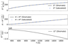 |
Fig. 1 Example of graphical output of the molecule database for corundum (A12O3(s)). Top panel: Entropy. Middle panel: Enthalpy. Bottom panel: Gibbs energy (chemical potential). Blue diamonds show tabulated values (upper two panels) and solid black lines the corresponding fitted Shomate function. |
4.2 Data processing, uncertainties, and extrapolation
The tabulated data are only available at discrete temperatures, with intervals of 100 K. To obtain continuous thermochemical data for any temperature, we used the tabulated enthalpies to fit Shomate parameters A, B, C, D, E, and F, via the respective Shomate equation (cf. Eq. (9)). Subsequently, we use the found values (A to E), the tabulated entropies and the respective Shomate equation (Eq. (11)) to find the last parameter G.
As an example, we show the thermochemical data of Al2O3(S) in Fig. 1. The top and middle panel show the entropy and enthalpy values of the species, respectively. We see that our Shomate fit (black solid line) retraces the tabulated data (blue diamonds) well. The bottom panel shows the Gibbs free energy derived from the other two properties.
In cases where the tabulated data contains discontinuities in the form of jumps at certain temperatures (commonly in reference-state data including multiple phases of a species), we fitted separate Shomate parameters for either side of the discontinuity. If the tabulated data do not span our entire temperature range of 300–6000 K, we applied a linear extrapolation for the Shomate enthalpy equation (parameters A and F) using the last three tabulated enthalpy values. The G parameter was fitted subsequently.
The uncertainty in thermochemical data can be very large, especially for solids. The reason for this is a combination of the limited precision of experimental measurements and errors introduced in the subsequent data processing, for instance by extrapolating measured data beyond the temperature range of the experiment. Regarding the measurement uncertainty, our data sources state an uncertainty of the order of 10% for the entropy at reference state for many minerals; for gases the uncertainty is generally much lower, often below 1% (for the exact values, we refer to the data sources themselves, Sect. 4.1). This uncertainty is propagated to the other values in the tables. Regarding the data processing uncertainty, Worters et al. (2018) and Woitke et al. (2018) studied the deviations between the thermochemical equilibrium constants of the species (kp) as stated in different data collections as a function of temperature. They found that only for 65% of the species the agreement between different sources is good over the entire temperature range, that is, better than 0.1 dex at high temperatures and better than 0.4 dex at low temperatures.
We did not take the uncertainty in the thermochemical data into account in the assembling of our thermochemical database, and it is not considered in any way in our simulations. It should, therefore, be kept in mind for the interpretation of our simulation results.
There are also uncertainties in the stellar elemental abundance data. For most rock-building elements, the estimated error of the given abundances is smaller than ±0.03 dex for the stars in our database (Brewer et al. 2016). We discuss the implications of these uncertainties in Sect. 6.2.3.
5 Computational solution
Our computational solution to the chemical equilibrium problem is provided as an open-source software on GITHUB5. It is written in Python and only relies on the standard Python libraries numpy, scipy and pandas6. Both the databases and minimisation code can be easily expanded to include more species or integrate a more sophisticated scientific approach, for instance by including an isolation fraction for the simulated solids or a thermochemical activity model.
5.1 Scope of our simulation
We limited the scope of our simulation in several areas. Most importantly, it is a purely thermochemical simulation. We do not consider disk profiles, disk dynamics, dynamical planet formation models or planet migration. The temporal development of the disk is only considered indirectly, in that we simulate a decrease in temperature, but do not set an absolute timescale for its evolution. The thermochemical approach is limited to equilibrium condensation, that is, we assume that all components of the system stay in chemical equilibrium for the whole temperature range of 6000–300 K, or, in any case, down to the temperature at which the planet is extracted from the disk. This is a twofold approximation: firstly, we assume that the cooling timescale of the disk is large compared to the thermochemical equilibration timescale, and secondly, we assume that no part of the condensates becomes isolated from the equilibration process, for instance, by being integrated into larger bodies. Furthermore, our model only includes ideal gases and solids. We do not include the condensation of trace elements.
Our scientific objective is the analysis of the composition of rocky planets; thus, it is limited to the solid materials found after condensation. While we do simulate the evolution of gas-phase species in the disk, they are not considered to be part of a forming planet. We only look at relative amounts of species and make no assumptions regarding absolute planet sizes.
5.2 Condensation simulation
The code’s main function is to compute the temperature-dependent equilibrium composition of a protoplanetary disk and to allow for the subsequent analysis of the results. This is realised by performing a sequence of Gibbs free energy minimisations at decreasing temperatures. As a result, the minimisation routine returns the relative amounts of each species – gaseous and solid – at each temperature step. This result matrix allows the inference of the temperature ranges in which a species is stable, and, therefore, expected to be present in the protoplanetary disk.
The code requires the specification of a start and end temperature, as well as the temperature increment, the disk pressure, the elemental abundance pattern in the disk, and the list of molecular species to be considered. The start and end temperature, as well as the temperature increment have no physical meaning; their computational impact is discussed in Appendix C.
The disk pressure is kept constant for the entire simulation, which means it is not automatically adapted to a decrease of gaseous material or temperature. Its value should be chosen in accordance with disk profiles. The elemental abundance pattern needs to be specified in terms of the normalised absolute number of atoms per element (see Sect. 4.1).
5.2.1 Molecule selection
A meaningful selection of the species to be included in the simulation is the most important, albeit most complex, aspect of the simulation. Our ideal is to include as few species as possible, in order to make the minimisation problem as numerically easy to solve as possible, thereby reducing the expected computation time and the likelihood of numerical errors. On the other hand, one wishes to find a stable mineral assemblage and hence would like to include all phases where thermodynamic data are available. Currently, there are >5000 minerals known to occur in nature; including all would likely lead to computational problems. The difficulty is determining the set of crucial species, that is, those that have a notable influence on the thermochemistry of the disk, for instance, by controlling the total pressure or otherwise determining condensation temperatures.
The total pressure is generally controlled by He and H2. On top of that, the simulation results will only be reliable if we include the most stable species at any sampled (T,p)-tuple for each element contained in the simulation. The most stable species carrying a particular element at a given (T,p)-value depends on the overall elemental abundance pattern; thus, compiling the list of species is typically an iterative process. The starting point of this process can be based on the extensive simulations of the Solar System, for instance by Lodders (2003), Woitke et al. (2018), and Wood et al. (2019).
5.2.2 Minimisation procedure
The minimisation at each temperature step is done using a trust region method, due to its known stability when solving bounded and constrained non-linear problems (Conn et al. 2000). The Gibbs function G(x, T, p), as defined in Eq. (15), is passed to the minimisation function as the target function, in combination with the non-negativity and number-balance constraints, the gradient (Eq. (28)) and Hessian matrix (Eq. (29)) in their respective capacity.
We derive the initial starting point x0 for the minimisation at the highest temperature of the simulation by solving the linear part of the Gibbs equation (Eqs. (22) and (23)) with a simplex method. We ignore the transcendental part of the function, but respect non-negativity and number-balance.
The vector c, as defined in Eq. (23), is constructed from the Shomate parameters of all included species, the specified temperature, and disk pressure. In all subsequent temperature steps, the solution at the previous temperature step is used as the initial guess input of the minimisation procedure.
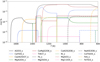 |
Fig. 2 Example of the progression of solid species of a simulation. The molar amount relative to the total molar content of the disk of each of the condensates included in the simulation is shown as a function of decreasing temperature in different line colours and styles, as denoted in the legend. See Appendix D for details on the included species. The simulation was run at a constant disk pressure of p = 10−4 bar and is based the solar elemental abundance pattern recommended by Lodders (2003). See Table B.2 for a summary of the simulation parameters. |
5.3 Simulation analysis and definition of the condensation temperature
We provide several functions to analyse the results of the condensation simulation. These analysis functions roughly fall into three categories. First, the basic parameters of the simulation (temperature range, included molecules, abundance pattern, and disk pressure) can be retrieved. Second, temperature progression curves of species can be plotted to analyse their amounts as a function of temperature and, in the case of solid species, their condensation behaviour. And third, the projected composition of a rocky planet as a function of its formation temperature can be studied.
Temperature progression curves are a powerful tool for analysing different aspects of planet formation. As an example, we show a plot of the relative molar amounts (mol − %)7 of all the solid species included in a simulation as a function of decreasing temperature in Fig. 2. The amounts are relative to the total molar content of the disk, that is, both gas- and solid-phase species  . From this figure, we can gather various information. For instance, the temperature of the first onset of condensation, the approximate total proportion of solids in the disk as a function of temperature, and the dominant contributors to a planet’s bulk composition at any given temperature, especially the distribution between typical planetary metal-core and silicate mantle components.
We implemented a computation of the condensation temperature of elements, as a common parameter to assess planet compositions. This is defined as the temperature at which 50% of the total amount of an element is bound in solid-phase species. As an example, we show the condensation of Ca in Fig. 3. The dark blue line denotes the fraction of Ca-atoms bound in gasphase species,  , in %, the light blue line the fraction bound in solid-phase species,
  The curves intersect at T = 1512 K, signalling the 50% condensation temperature of Ca.
Additionally, we define a ‘condensation temperature’ of specific solid-phase molecules (synonymously used for minerals) in order to analytically assess the appearance of condensates and sequences of phases containing specific elements. This value is, however, far less distinct than the condensation temperature of an element. There are two reasons for this: firstly, the maximum amount of a particular phase is not known a priori and depends on the temperature range considered; secondly, phases often disintegrate at lower temperatures in favour of more stable phases. This behaviour is exemplified in the left panel of Fig. 4 for perovskite (CaTiO3(s)), which is superseded by Ti4O7(s). Some species show even more complex condensation behaviours, involving successions of increases and decreases in their relative amounts. This is demonstrated in the right panel of Fig. 4 for forsterite (Mg2SiO4(s)), which is part of the intricate Mg-Si-chemistry in the protoplanetary disk. Irrespective of the precise curve shape, we only compute one condensation temperature per species, based on the 50% level of the local maximum closest to the first onset of condensation. If a species is present in such small quantities that it cannot be distinguished from numerical noise, it is assumed to not have condensed in the simulation, and therefore no condensation temperature is reported.
For the analysis of the composition of an exoplanet itself, we use the code’s output of relative molar amounts of the chemical species that are stable in chemical equilibrium as a function of temperature. We convert this information into the relative amounts of the individual elements bound in solid species, using the structural formulae of the species. This procedure results in a temperature-series of the elemental composition of solid material in the disk. As default, we give the resulting composition in units of wt − %, meaning the total mass of one element bound in solid species relative to the total mass of all elements in solid species, using the atomic weights data specified in Sect. 4.1. To get the composition of an individual planet out of the temperature series, we have to specify its ‘formation temperature’. This temperature defines the point, at which the planetary material is taken out of the chemical equilibrium of the disk. This does not necessarily mean that the planet is fully formed at this temperature, nor that it corresponds to the final disk temperature at the location of the planet. It is sufficient that the planetesimals have become so large that their interiors are effectively shielded from the disk chemistry. For instance, the depletion pattern of volatile elements in the Earth suggests a formation temperature between 1100 and 1400 K (Wang et al. 2019a; Sossi et al. 2022). We discuss our different models connecting the formation temperature to the planet’s composition in Sect. 7.1.
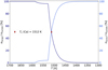 |
Fig. 3 Example of the condensation curve and condensation temperature of a specific element, here Ca. The dark blue curve shows the fraction of Ca atoms bound in gas-phase species, the blue line shows the fraction of Ca atoms bound in solid-phase species. The T-value of the intersection at 50% of atoms in gas- and solid-phase signifies the 50% condensation temperature. |
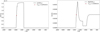 |
Fig. 4 Examples of different types of condensation behaviours of solid species. We show the relative molar amount of the species present in the protoplanetary disk as a function of decreasing temperature to demonstrate our definition of 50% condensation temperatures. Red diamonds show the computed 50% condensation temperatures. Left panel: progression of perovskite CaTiO3(s) (condensation and subsequent disintegration). Right panel: progression of forsterite Mg2SiO4(s) (varying relative amounts). |
6 Condensation temperatures and their dependence on pressure and element abundance
We used our code to look at condensation temperatures and their variability. The condensation temperatures of rocky species give a first idea of the building blocks of a planet, because only material that has condensed at the formation temperature of a planet can be accreted from the protoplanetary disk. The condensation temperature of elements takes this idea to a slightly more abstract level, as we are not looking at the specific material that can be accreted onto a planet anymore, but rather think about the final elemental composition of the planet, even after the original planetesimals have undergone chemical changes in the formation and consolidation of the planet, for instance due to thermal processes. This relies on the assumption that while the specific molecules that have been accreted might not be found in the final planet in their original form, their elemental proportions will be retained. Finally, the variability of the condensation temperatures gives an indication as to how applicable our understanding of the connection between the formation and composition of the Earth is to different planet formation regions in the disk and to exoplanetary systems.
To validate the results of our code externally, we compared them against benchmark results from the literature. In Sect. 6.1 we show our computed condensation temperatures of common rocky species (Sect. 6.1.1) and of elements (Sect. 6.1.2) for a Solar System elemental abundance pattern at a constant pressure, and compare them against the results by Lodders (2003) and Wood et al. (2019). In Sect. 6.2 we explore the variability of the condensation temperatures of elements as a function of the disk pressure and the stellar elemental abundance pattern.
6.1 Condensation temperatures for a solar elemental abundance pattern and constant pressure
First, we analyse the condensation temperatures of species and elements that can be derived for the solar elemental abundance pattern at the disk pressure associated with the formation of Earth. In order to also use our results as a benchmark test for our code, we used the same system parameters that were used in the studies we compare our results against, even if these values are not necessarily in line with the currently most accepted ones.
Namely, we used the Solar System elemental abundances pattern as reported by Lodders (2003) and a disk pressure of 1 × 10⁻⁴ bar, which was found to represent the total pressure in the solar nebula near 1 AU by Fegley (2000), and which was also used for the simulations of Lodders (2003) and Wood et al. (2019). Our simulation covered a temperature range from 2000 to 300 K, with a resolution of 1 K. The number of species included in our simulation (47 gases + 25 solids) was much smaller than in the comparison studies. The simulation parameters are summarised in Table B.2.
We estimate very conservatively that different codes should return condensation temperatures of molecules within 100 K of each other and condensation temperatures of elements within 20 K for a given disk pressure and abundance pattern. This presumes that the most common elements and the majority of the most stable molecules are included in the simulation. This estimate is based on our experience regarding the response of our own code to variations in the molecule selection, the thermochemical data, and the definition of the condensation temperatures, in the case of molecular species.
6.1.1 Condensation temperatures of rocky species
For the validation of our simulated condensation temperatures of common rocky species, we used the benchmark results of the seminal work by Lodders (2003). Their results have been computed with the CONDOR-code, which is not publicly available. Their thermochemical database contains 2000 gas-phase species and 1600 solids, which are all considered for the simulation. In their code, the chemical equilibration is based on equilibrium constants of formation, rather than Gibbs free energy, and the reported condensation temperatures pertain to the point at which the computed activity of a solid species reaches unity (Lodders 2003). Visually, this point would typically correspond to the onset of condensation, that is, the initial sharp change in gradient seen in our condensation curves of molecules (see Fig. 4 as an example). Depending on the slope of the curve, this temperature might easily be 20 K higher than our 50% condensation temperature, as defined in Sect. 5.3.
Keeping this in mind, we found a high degree of agreement between the two sets of values, as shown in Table 1. Our condensation temperatures are mostly within ±50 K of the literature values. Our values are on average lower than those of (Lodders 2003), confirming our expectation based on the different definitions of the condensation temperature.
Regarding condensation sequences, we found that the order in which the molecules are expected to condense has been reproduced well with our code. The slight observed differences, as well as our failure to condense grossite (CaA14O7), are likely due to the fact that our code does not include solid solutions. The solid solutions of the olivine and pyroxene mineral groups especially will lead to a shift in the Mg budget, potentially affecting the condensation of most of the shown species.
In conclusion, the found agreement between the two codes is much better than our conservative estimate. The combination of vagueness of the definition of the condensation temperature of a molecule and the large uncertainty in the thermochemical data itself (see Sect. 4.2) suggests that one should not attach great meaning to their exact simulated values.
Comparison of condensation temperatures of some common planetary species.
6.1.2 Condensation temperatures of elements
In contrast to the condensation of a rocky species, the 50% condensation temperature of the elements (the temperature at which 50% of the element is bound in solid species) is very sharply defined, since its maximum amount is known a priori from the given elemental abundance (cf. Sect. 5.3). Additionally, the selection of species is less influential in the equilibrium computation, since the elements tend to only be exchanged between different solid-phase species after the initial onset of condensation, but do not return to gas-phase species. Accordingly, not including a particular species does not affect the amount of the element being bound in solid-phase species, and consequently the 50% condensation temperature.
Furthermore, the condensation temperatures of elements enable us to easily estimate the composition of a rocky planet. Most elements condense (10-90%) within a T-interval smaller than 100 K. This implies that there is hardly any of the element in solid form at temperatures above the 50% condensation temperature, whereas all of it is in solid form at temperatures below. Hence, if the formation temperature of a planet is above the 50% condensation temperature of an element, it will not contain significant amounts of this element. Otherwise, the element will have a similar relative abundance in the planet as in its host star. If the formation temperature of the planet is close to the condensation temperature of an element, this element will likely be depleted to some degree in the planet.
For the comparison, we again used Lodders (2003), as well as the more recent study of Wood et al. (2019). The latter applied the PHEQ code, developed by and described in Wood & Hashimoto (1993), which is very similar in its thermochemical approach to our code.
The agreement with Lodders (2003) and Wood et al. (2019) for the condensation temperatures of major rock-forming elements are excellent, as shown in Table 2. The average discrepancy from the mean condensation temperature of each element is below 5 K and the largest deviation is below 15 K (cf. Fig. 5).
We conclude that the 50% condensation temperatures of the most common planet-building elements are not sensitive to details of the used condensation algorithm. In other words, even our very simplistic approach with only a few included species, will return results with a projected error below ± 10 K, for a given elemental abundance pattern and disk pressure.
Comparison of 50% condensation temperatures of major rock-forming elements.
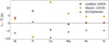 |
Fig. 5 Graphical comparison of deviation of 50% condensation temperatures of the major rock-forming elements, minus the mean over the three values for each element. |
6.2 Dependence of the condensation temperatures of elements on system parameters
We explored the variability of the condensation temperature of elements as a function of disk pressure and elemental abundance pattern. While it has been widely acknowledged that the chemical processes in the protoplanetary disk are controlled by its elemental composition and especially its C/O and Mg/Si ratio (Bond et al. 2010b; Carter-Bond et al. 2012; Thiabaud et al. 2014; Moriarty et al. 2014; Dorn et al. 2019; Bitsch & Battistini 2020), the condensation temperatures of the elements are sometimes implicitly treated almost as material constants, at least within certain limits of system parameters (see e.g. Wang et al. 2019a,b; Spaargaren et al. 2020).
In Sect. 6.2.1 we explore the influence of the disk pressure, and in Sect. 6.2.2 we analyse the effect of a variation in the elemental abundance pattern. In Sect. 6.2.3 we briefly discuss implication of our findings.
6.2.1 Dependence on disk pressure
The condensation temperatures of elements are often reported for a total disk pressure of 1 × 10⁻⁴ bar. In general, however, the disk pressure depends both on the radial distance from the central star, the vertical distance from the mid-plane, and the total material within the system (Fegley 2000).
We varied the disk pressure logarithmically between 1 × 10⁻⁶ bar and 1 × 10⁻¹ bar, while keeping all other parameters of the simulation constant. Depending on the disk model, this range of pressure values might correspond to a radial distance range from 0.1 to 5 AU in a Solar-System-like disk (Fegley 2000), that is, distances within the water snow line, where we expect to find rocky planets.
As shown in the top panel of Fig. 6, we found an overall trend of a higher disk pressure corresponding to a higher condensation temperature of the elements. Raising the pressure in a system where nothing else is changed, is equivalent to increasing the particle concentration. This implies an increase in the reaction rates. Since the pressure raises the effective concentration of all species equally, we found a quantitatively very similar relation between the disk pressure and the condensation temperature for all analysed elements, except for S.
This can be seen particularly clearly in the bottom panel of Fig. 6, where we show the deviation of the condensation temperature of an element at a given disk pressure from the element’s mean condensation temperature within the analysed pressure range. For the analysed pressure range all species have their mean condensation temperature at roughly the same pressure (between 4 × 10⁻⁴ bar and 5 × 10⁻⁴ bar). Also, the deviation from this mean is similar for all elements at each disk pressure. On average, the condensation temperature of all elements except for S increases by (357 ± 57) K over the analysed five orders of magnitude in disk pressure. S behaves differently, its condensation temperature does not change at all over the pressure range8.
The consistency in pressure versus condensation temperature relations between the different elements has implications for the analysis of planet formation at different radial locations within the protoplanetary disk. In disk models, both the mid-plane temperature and the disk pressure decrease with increasing distance from the central star. Generally, when simulating planet formation, both pressure and temperature are considered in combination. However, since the disk pressure affects the condensation temperatures of all elements very similarly, the variation in disk pressure does not change the equilibrium chemistry and equilibrium composition as a function of temperature qualitatively, but only shifts the equilibrium composition to higher temperatures (for an increased pressure) or to lower temperatures (for a decreased pressure). The small variations in the pressure response of the elements’ condensation temperature will likely be rendered insignificant by the fact that a planet does not comprise material of one specific (T-p)-equilibrium condition but rather a mixture over a range of conditions. As shown in Fig. 6, the greater the change in pressure, the larger the difference in Tc between the elements. Our argument is therefore only valid for small pressure ranges.
6.2.2 Dependence on the elemental abundance pattern
There have been many studies assessing the diversity of exoplanetary compositions as a result of the changed equilibrium chemistry in a protoplanetary disk, due to variations in its elemental abundance pattern (e.g. Bond et al. 2010b; Carter-Bond et al. 2012; Thiabaud et al. 2014; Moriarty et al. 2014; Dorn et al. 2019; Bitsch & Battistini 2020; Jorge et al. 2022). Certain element ratios control which molecular species will form out of the available elements. Different molecules can have vastly different condensation temperatures even if they consist of similar elements. The species in which an element is predominantly bound, generally determines its 50% condensation temperature.
To systematically analyse the influence of the elemental abundance pattern on the condensation temperatures of the elements, we ran condensation simulations for synthetic abundance patterns, only varying one key element ratio at a time. We explored the role of the overall metallicity and the element ratios C/O, Mg/Si, Fe/O, and Al/Ca. We specify metallicities logarithmically and normalised to solar values:
![$\left[ {{{\rm{M}} \mathord{\left/ {\vphantom {{\rm{M}} {\rm{H}}}} \right. \kern-\nulldelimiterspace} {\rm{H}}}} \right] = \log \,{\left( {{{{N_{\rm{M}}}} \over {{N_{\rm{H}}}}}} \right)_{{\rm{star}}}} - \log \,{\left( {{{{N_{\rm{M}}}} \over {{N_{\rm{H}}}}}} \right)_{{\rm{sun}}}}, $](/articles/aa/full_html/2023/08/aa44850-22/aa44850-22-eq33.png) (30)
(30)
where NM is the sum of the relative number of atoms in the system of all elements larger than He, and NH the relative number of H atoms. All other element ratios are given as non-normalised number ratios, for instance, ‘C/O’ means
 (31)
(31)
As a basis for our analysis, we used the Brewer et al. (2016) catalogue of 1617 F, G, and K stars. To ensure the reliability of the abundance data, we only took stars into account whose spectra have a signal-to-noise ratio (S/N) larger than 100. Furthermore, to avoid giant stars, we excluded all stars with log ɡ ≤ 3.5 (compare Harrison et al. 2018). We used the remaining 964 stars to (1) generate a representative abundance pattern as a starting point for the element ratio variations, (2) determine the parameter ranges of the element ratios we were interested in, and (3) pick roughly 100 stars, covering the whole parameter space, to verify that any trends found in the analysis of the synthetic data are also followed by the real stellar data. Figure 7 shows the parameter ranges (Teff versus metallicity, C/O versus Al/Ca, and Mg/Si versus Fe/O) covered by the Brewer et al. (2016) stars, and the distribution of the sample of comparison stars.
For most variations of the element ratios, we kept the abundance of one element constant in our representative abundance pattern, and only varied the other. For the overall metallicity, only the H abundance was changed. For the Al/Ca, Mg/Si, and Fe/O ratios, Al, Mg, and Fe were varied, respectively. The C/O ratio was treated differently. In the studied stellar sample, there is a strong correlation between the C/O ratio and the ratio of O to the sum of other abundant elements, such as Mg, Si, and Fe. In order to avoid a distortion of the analysis due to an unrealistic abundance pattern of the synthetic data, we approximated this correlation with a parabola, as shown in Fig. 8, and adapted both the C and O abundance accordingly.
Our tests show that an element ratio can affect the condensation temperatures in different ways. We can differentiate the effects in terms of the number of affected elements, and the curve shape of the correlation between the ratio and condensation temperature. Table 3 shows the summary of our findings. The overall metallicity and C/O ratio have the most profound impact on the condensation temperatures. These two variations stand out, because (1) they affect a large number of elements, (2) the magnitude of change in condensation temperatures is high, and (3) the correlation between the ratio and the condensation temperature of all affected elements is systematic. We therefore limit our discussion to these two parameters and only cover the others in a cursory fashion.
In Fig. 9, we show the influence of the overall metallicity of the system on the condensation temperatures of a selection of common elements. The coloured foreground markers represent the simulation result for the synthetically varied metallicity, the grey background markers show the simulation results of the random sample of comparison stars. The figure clearly demonstrates a linear correlation between the logarithmic metallicity and condensation temperature for all elements. We found an increase in condensation temperature between 52 K (Fe) and 117 K (Al) over the covered metallicity range. Despite the fact that the abundance patterns of the comparison stars are quite diverse (cf. Fig. 7), the log-linear correlation between metallicity and condensation temperatures can also be found there9. The median deviation of the condensation temperatures from the interpolation curve of the synthetic simulation results is below 20 K for all the elements.
The effect of the overall metallicity is reminiscent of the effect of disk pressure variations, seen in Sect. 6.2.1. This is unsurprising as both variations effectively change the relative number of rock-building particles per volume, that is, the chemical reaction rates.
We have found a similar log-linear correlation for the Fe/O ratio, which does, however, only affect the condensation temperature of Fe itself. Again, we suspect this to be explainable by the fact that we increased the partial pressure of Fe. Since its dominant solid species in our simulation is pure solid iron, this increased partial pressure does not shift the balance of any other chemical reaction. The result would apply analogously to similar condensation patterns, where the dominant solid species do not include any other elements, such as the Ni condensation.
In Fig. 10, we show the influence of the C/O ratio on the condensation temperature of some common elements. Again, the synthetic simulation results are depicted with coloured foreground markers, the comparison stars with grey background markers. It is important to note that in this figure the effect of the metallicity, as described above, has already been removed from the results. The order of magnitude of the change in condensation temperature caused by the variation of the C/O ratio is similar to that of the metallicity. There are, however, also several qualitative differences. The most obvious difference is that an increase in the C/O ratio causes a decrease in condensation temperatures, in contrast to the increase caused by a higher metallicity. Also, while there certainly seems to be a systematic effect of the C/O ratio on all condensation temperatures, the correlation is not log-linear. Finally, while the metallicity affected all condensation temperatures, the C/O ratio only affects elements whose dominant species contain O, for instance, the condensation of Fe and Ni are unaffected.
The expected correlation mapped out by the synthetic data is followed exceptionally well by the real data simulations, especially for the range 0.3 ≤ C/O ≤ 0.7. For the whole parameter range, the median deviation from the expected curve is below 10 K for all elements. For C/O values below 0.3, the real data condensation temperatures of Al and Ca do not follow the synthetic data well. This is caused by the superposition of the influence of the Al/Ca ratio. The diverging systems coincidentally all feature a particularly low Al/Ca ratio. Our tests with synthetically varied Al/Ca ratios have shown that it causes a roughly log-linear increase of the Al condensation temperatures and a step-function increase for Ca (see Fig. 11, left panel). This explains why the condensation temperatures of Al shown in Fig. 10 gradually taper off from the expectation curve, whereas the Ca condensation temperatures suddenly jump to values more than 100 K below the expectation.
These differences between the effect of the variations in metallicity and in the C/O ratio allude to different underlying mechanisms. We have argued that an increase in metallicity implies increasing the number of all reactants per volume, thereby increasing all reaction rates. In contrast, changing the C/O ratio tilts the reaction balances in the formation of many major species, by only changing the availability of one of the reactants or by changing them to different degrees. The effect of a changed reaction balance is far more difficult to predict than the effect of globally increased reaction rates. Reaction balances are particularly strongly affected when the involved element ratios in a system are typically close to unity, because then a change in the ratio can imply that the availability one of the reactants is exhausted before the other, inhibiting this reaction. This is the case for the C/O, Mg/Si, and Al/Ca ratios.
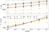 |
Fig. 6 Dependence of the 50% condensation temperature (Tc) of elements on the disk pressure. Markers represent simulated condensation temperatures, and corresponding dashed lines are only to guide the eye. Colours, as denoted in the legend, are the same for both panels. All simulations use the solar elemental abundance pattern recommended by Lodders (2003). Top panel: 50% condensation temperature of major planet-building elements as a function of different disk pressures. Bottom panel: deviation of the 50% condensation temperature from the respective mean condensation temperature. |
Summary of the influence of the variation in different element ratios on the condensation temperature of elements.
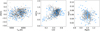 |
Fig. 7 Parameter range of the Brewer et al. (2016) stellar database. Grey background markers represent all stars with logɡ > 3.5 and S/N > 100 of the database, and light blue foreground markers represent the stellar sample studied here. Left panel: effective temperature versus metallicity. Middle panel: C/O ratio versus Al/Ca ratio. Right panel: Mg/Si ratio versus Fe/O ratio. |
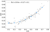 |
Fig. 8 Correlation between the C/O and Σ/Ο, where Σ = NMg + NSi + NFe, + NCa + NAl. Grey background markers represent the studied stellar sample, and the dotted line shows the fit quadratic fit to the data. The light blue foreground markers show the synthetic data for the C/O analysis. |
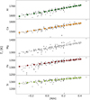 |
Fig. 9 Correlation between the overall metallicity of the system and the condensation temperature of some major planet-building elements. The coloured circles in the foreground show the simulation results of the synthetic abundance patterns, and the grey circles in the background show the simulation results of a representative subset of approximately 100 stars from the Brewer et al. (2016) database. All simulations were run at a constant disk pressure of p = 10−4 bar. |
6.2.3 Implications of the variability in condensation temperatures
Our findings regarding the variation of the condensation temperatures of elements have several implications. Most importantly, a combination of variations in pressure and elemental abundance pattern, even over a moderate parameter range, can easily change the condensation temperatures of elements by more than 100 K. This needs to be taken into account, when they are used to estimate planet compositions in other stellar system, for instance when applying the elemental devolatilization pattern of the Earth to exoplanets (Wang et al. 2019b; Spaargaren et al. 2023) or in the context of white dwarf pollution (Jura & Young 2014; Farihi et al. 2016; Harrison et al. 2018; Wilson et al. 2019; Bonsor et al. 2020; Veras 2021; Xu & Bonsor 2021).
We have, however, seen that the overall metallicity and the disk pressure affect all elements very similarly. Neglecting those will likely not be of great consequence to any derived exoplanetary compositions. That is to say, the computed element ratios would agree well with a model taking these parameters into account over the whole simulation range, but these ratios would be predicted for shifted radial distances.
Other variations in the elemental abundance pattern, however, cause more unpredictable changes to the condensation temperatures of some elements. As a result, both the sequence in which the elements condense, as well as the difference in their condensation temperatures can be significantly altered. These changes entail substantial qualitative deviations in the most likely composition of a planet expected to form in a given system compared to its Solar System analogue. We explore this point further in Sect. 7.
Furthermore, our findings give us an idea of the potential influence of the uncertainty of stellar abundance measurements. While the uncertainties of the abundances of most planet-building elements might be lower than ±0.03 dex for many well-studied F, G, and К stars (Brewer et al. 2016), and even an uncertainty at the ±0.01 dex level seems feasible for these stars (Bedell et al. 2014), the situation is generally much worse. For M-dwarfs, where abundance measurements are in their infancy, typical errors exceed ±0.1 dex (Souto et al. 2017). As we see in Fig. 10, a difference of ±0.1 dex in the C/O ratio can signify a difference of some tens of Kelvins in the condensation temperature of certain elements, at least at the upper end of our tested range, that is, C/O ≥ 0.5. An in-depth analysis of the impact of uncertainty is available in Hinkel & Unterborn (2018).
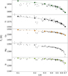 |
Fig. 10 Correlation between the C/O ratio and the condensation temperature of some major planet-building elements, corrected for the metallicity effect. The coloured circles in the foreground show the simulation results of the synthetic abundance patterns, and the grey circles in the background show the simulation results of a representative subset of approximately 100 stars from the Brewer et al. (2016) database. All simulations were run at a constant disk pressure of p = 10−4 bar. |
 |
Fig. 11 Correlation between element ratios and the condensation temperatures, corrected for the metallicity and C/O effect. The coloured circles in the foreground show the simulation results of the synthetic abundance patterns, and the grey circles in the background show the simulation results of a representative subset of approximately 100 stars from the Brewer et al. (2016) database. All simulations were run at a constant disk pressure of p = 10−4 bar. Left panel: influence of the Al/Ca ratio on the condensation temperature of Al and Ca. Right panel: influence of the Mg/Si ratio on the condensation temperature of Mg and Si. |
7 Exoplanet compositions
We now look at the bulk composition of rocky planets around chemically different stars. To emulate the dynamical formation of planets we compare different methods of assembling the solid material from our equilibrium condensation simulation. To externally validate our results and qualitatively assess the merits of our composition models, we compare them against the n-body simulations of Bond et al. (2010b; hereafter B10).
7.1 Derivation of planet compositions
Our underlying disk model is vastly simplified. The only parameter changing within our disk is the temperature, which is a proxy for distance from the central star. For our study, we are not interested in an exact temperature-distance relation but only in qualitative tendencies. We keep the pressure constant at a value of 1 × 10⁻⁴ bar. This pressure value is often assumed for the formation of Earth (Fegley 2000; Lodders 2003; Wood et al. 2019). In this context, however, the choice was arbitrary. As shown above in Sect. 6.2.1, variations in disk pressure affect the condensation of all species very similarly, especially if the expected variation in pressure is small10.
To derive the bulk composition of a planet for any given formation temperature (see above, Sect. 5.3), we use three different methods of assembling planetary material to emulate planet formation via accretion. While our models are loosely rooted in the idea of planetary accretion from within the planet’s Hill sphere (see e.g. Pollack et al. 1996; Kley 1999), we only use them to bypass computationally expensive n-body simulations. That means there is no correspondence between the expected physical size of the planet and the diversity of the material assembled in our code; we instead made the latter match the results of the и-body simulation. As illustrated in Fig. 12, we compare two differently shaped planetary feeding zones (FZs) to a model without a FZ.
In the simplest approach, the planet is only made up of the solid material that is stable at the planet’s formation temperature, with the relative amounts dictated by the thermochemical equilibrium at that temperature. This approach corresponds to taking an infinitesimally thin section of the elements-temperature-progression described in Sect. 5.3. It is illustrated in the bottom panel of Fig. 12, where the x-axis represents the temperature decreasing with distance from the central star, all material except that at Τ = Tcentral is discarded.
The first FZ is an equal weights temperature band, illustrated in the middle panel of Fig. 12, later referred to as ‘boxcar FZ’. We specify the width of the temperature band, add up the elemental equilibrium compositions within the temperature range, and normalise the result. This normalised result is taken to be the planetary composition at the central temperature of the band. Since a lower temperature generally entails a higher total amount of solids in the equilibrium, it follows that the lower-temperature edge of the band effectively has a stronger influence on the resulting planetary composition than the higher-temperature edge.
The second type of FZ is a Gaussian profile, as illustrated in the top panel of Fig. 12. Here, the total material at each temperature is first multiplied by a normal distribution with a specified standard deviation, σ, and subsequently added up. The argument regarding more solid material being present at lower temperatures also applies to this FZ. The width of the FZ is given by 2σ. The location of the peak of the normal distribution gives the planetary formation temperature.
For both of these types of FZ, the effect of a ring geometry on the amount of available material is not taken into consideration for the final planetary make-up. That means we neglected the fact that a lower temperature corresponds to a greater distance from the star. A larger radius of the ring implies more material with that particular composition being available for accretion onto the planet. To quantify this geometric effect, we would have to connect our temperature profile to specific distances, which is not part of our simplified model.
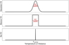 |
Fig. 12 Illustration of the three different FZ models for creating a planet’s composition at a given temperature. The x-axis denotes the temperature, or equivalently the distance from the star. Top panel: Gaussian profile. Middle panel: Boxcar profile. Bottom panel: No FZ model. |
7.2 Application and comparison study
Following the approach of В10, we analyse the predicted planetary compositions with our simplified disk model for chemically diverse stars, delineated primarily by differences in their C/O ratios. In particular, we explore the simulated compositions of a rocky planet formed around a low-carbon star (HD 27442), around a medium-carbon star (HD 17051), and around a high-carbon star (HD 19994), using the three different planetary FZ models described above. The physical properties of the stars are listed in Table 4. We use the elemental abundances of these stars as reported by В10, in order to facilitate the comparison of the results. It should be noted, though, that these abundances have later been found to be inaccurate, especially the C/O ratios are vastly overestimated (Fortney 2012; Nissen 2013; Teske et al. 2014; Brewer & Fischer 2016). Based on more recent studies of stars in the solar neighbourhood (e.g. Brewer et al. 2016), all of the C/O ratios analysed in this section would be classified as moderately high or high.
We compare our results against the results of В10. They simulated the composition of rocky planets by combining a chemical equilibrium condensation with a dynamical accretion simulation. The chemical equilibrium condensation was done with the HSC suite. The T-p input parameters were based on the Hersant et al. (2001) temperature-pressure-profile for the mid-plane of the protoplanetary disk11. The solids formed in equilibrium at the specified temperature and pressure constitute the planetary building blocks for the dynamical n-body simulation, which was done using the SYMBA integrator (Duncan et al. 1998). They ran four accretion simulations for each of the studied stars, slightly varying the initial distribution of planetesimals, and recorded the composition of the final planets as the sum of all accreted material. Each simulation run returned between zero and three planets per star. For each star, we show the planet compositions in order of formation distance across the whole set of the B10 simulations. This illustrates representative compositional patterns as a function of distance, and captures their variability due to dynamics.
Physical parameters of stars analysed in this section.
7.3 Results for chemically diverse systems
Figures 13 to 15 show the comparisons among our results of planet compositions for the three stars and to the B10 results. We describe them in more detail in the following subsections. Each figure contains four panels, showing the bulk composition of a planet (in wt – %) simulated to form around the respective star. The top panel shows the discrete results of the B10 simulation as a function of distance, the second panel from the top shows our composition for a Gaussian FZ, the third panel shows our simulation for a boxcar FZ, and the bottom panel shows the composition without any FZ. Where possible, we group the B10 planets with similar composition and indicate roughly which section of our simulation best corresponds to them with arrows between the top most and second panel.
7.3.1 Low carbon abundance
In Fig. 13 we show the system of HD27442, which has the lowest carbon abundance of the three analysed systems (C/O = 0.61). The elemental abundance pattern of this star is similar to the solar values. This implies that the simulated planets can be expected to also resemble the inner planets of the Solar System in bulk composition. No S abundance is reported for HD 27442. Since its C/O ratio is far below 1, S species are not expected to play a major role in the equilibrium chemistry (see footnote 8 and Sect. 7.3.3). We therefore excluded all species containing S from the simulation of this system.
Starting closest to the central star, two planets from the B10 simulations formed at 0.33 and 0.35 AU with similar compositions of mostly O and Al, significant amounts of Mg, Ca, and Si. We find a very similar composition in our simulation without a FZ at or slightly below 1400 K. The boxcar FZ, with a width of 100 K, produces a slightly different composition for this formation temperature, with a reduced Mg-content. This is caused by mixing in material from the higher-temperature regions, where only Al-Ca-O species have condensed. We cannot reproduce the composition of the two innermost planets with our Gaussian profile, because it does not create a region that contains Mg but no Fe.
At intermediate distances, we find a group of five planets in the B10 simulation with similar O and Si contents as the innermost planets, but with ever increasing Fe amounts. These planets formed between 0.36 and 0.52 AU, which seems to correspond to the location Fe snow line in the B10 simulation. Due to the very abrupt condensation of Fe at T ≈ 1360 K, we cannot reproduce this planetary composition without resorting to a FZ. The gradual change in planet composition can be reproduced with both FZ models. The boxcar model would profit from a larger FZ width than the one used here, though.
At greater distances, we find a group of three planets in the B10 simulation that can be characterised by their large content of Fe, Mg, O, and Si. These planets formed between 0.52 and 0.77 AU. As shown in our continuous simulations, the composition of the solids in the disk converges to these specific ratios, which are in accordance with the stellar elemental abundance ratios. This is due to the fact that we now look at planetary formation temperatures below the condensation temperatures of the main planetary components. Once we enter this region, the FZ model becomes obsolete, as the material to either side of the central temperature is identical.
There is one final planet left in the B10 simulation that has no correspondence with our continuous simulation. It formed at the greatest distance from the star, but its composition rather resembles the second group of planets. The formation of this planet requires substantial dynamical processes, likely in the form of planet migration, which cannot be emulated by our simple FZ model.
7.3.2 Medium carbon abundance
In Fig. 14 we show the planets simulated to form around the star HD17051, which has an intermediate carbon abundance among the analysed systems (C/O = 0.87). Closest to the central star, we see five B10 planets with almost identical compositions. They formed between approximately 0.3 AU and 0.4 AU. They contain a large fraction of O, similar amounts of Al and Ca, and a small amount of Si. We find the same composition in our simulation for all three types of FZs between roughly 1500 and 1400 K. For the Gaussian FZ, though, the region corresponding to the composition of the B10 planets is very narrow, which is difficult to reconcile with the consistent compositions returned by the n-body simulation. The model without a FZ has a broad plateau of the same composition as the B10 planets. The boxcar FZ does not have such a broad plateau, but shows a section with a sufficiently constant composition to be compatible with the formation of similar planets over an extended range of distances.
At greater distances, we identify two B10 planets with very similar composition that are vastly different from the first group. These planets are dominated by their high Fe content, exceeding 50% of the total weight of the planet, and suggesting a very extensive planetary core. The remaining composition is made up of O, Mg, and Si, with only small contributions of Ni, Ca, and Al. In contrast to the HD 27442 system, this group of planets has not formed in region of the convergence composition of the disk. We can clearly see in our simulations that the composition changes significantly all the way down to approximately 600 K, when S condenses.
Both the high similarity of composition over a fairly large distance range, as well as the deviation from it in the form of a slight increase in Mg, O, and Si can be seen in our three continuous models in the temperature range from approximately 1300 – 1200 K. Both the Gaussian and the boxcar profile reproduce the gradual changes in the composition of the B10 planets. The composition without a FZ compares less favourably, because at the onset of the Mg and Ni condensation, it changes are very rapidly and strongly, and at lower temperatures, it stays constant.
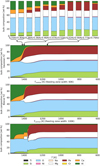 |
Fig. 13 Predicted bulk composition (in wt – %) of a rocky planet simulated for the elemental abundance of HD 27442 (low carbon system). Top panel: B10 planet composition results from four separate simulation runs. We also show our simulations: with a Gaussian FZ (second panel), a boxcar FZ (third panel), and no FZ (bottom panel). The arrows between the first two panels indicate roughly the location of the best correspondence between the Bond simulation and ours. |
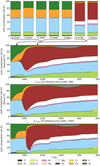 |
Fig. 14 Predicted bulk composition (in wt-%) of a rocky planet simulated for the elemental abundance of HD 17051 (medium carbon system). Top panel: B10 planet composition results from four separate simulation runs. We also show our simulation: with a Gaussian FZ (second panel), with a boxcar FZ (third panel), and with no FZ (bottom panel). The arrows between the first two panels indicate roughly the location of the best correspondence between the Bond simulation and ours. |
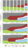 |
Fig. 15 Predicted bulk composition (in wt-%) of a rocky planet simulated for the elemental abundance of HD 17051 (high carbon system). Top panel: B10 planet composition results from four separate simulation runs. We also show our simulation with a Gaussian FZ (second panel), with a boxcar FZ (third panel), and with no FZ (bottom panel). The arrows between the first two panels indicate roughly the location of the best correspondence between the Bond simulation and ours. |
7.3.3 High carbon abundance
Finally, we show the planets simulated to form around the highcarbon star HD 199944 in Fig. 15. Based on the elemental abundance data we use for this simulation, the star has the exceptional C/O ratio of 1.26. We expect a completely altered disk chemistry for systems with C/O ratios exceeding unity. All O-atoms are bound to C-atoms to form highly stable CO gas molecules (Mollière et al. 2015; Woitke et al. 2018). Accordingly, O is no longer available for the solid-phase chemistry, inhibiting the condensation of some of the most common species in planet formation, such as Al2O3, CaAl12O19, and MgSiO3. Because all O is bound to CO, no O is available to bind with H2 to form H2O and the system becomes highly reducing. This means that all Fe is in reduced state and that some Si occurs in metal instead of silicates. A C/O ratio exceeding 1 also means that free C is available to form exotic phases like SiC or free C in form of, for example, graphite. In high C/O systems, S replaces O as anion, which leads to a much higher condensation temperature of S as it condenses with Ca into refractory phases like oldhamite (CaS). Although the solar C/O is approximately 0.5, some portions of the early Solar System apparently had C/O ratios close to 1 as it is evident from the presence of CaS in reduced enstatite chondrites or exotic elemental ratio patterns of the rare Earth elements in ordinary chondrite chondrules (Pack et al. 2004). A planet with a bulk C/O > 1 would certainly not allow the presence of liquid water and thus would likely be hostile for life.
From a practical, computational point of view, it should be noted that not many S species are taken into account in condensation simulations, due to their limited importance in solar-like systems. For instance, B10 only considers the solid S species FeS, MgS, and CaS; we only added Al2S3 to this selection12. This means that the simulations likely do not reflect the true disk chemistry of a C-rich system.
As expected, the composition of the simulated planets is completely different from the planets discussed so far. Starting again closest to the central star, we find two B10 planets only containing C and Si. They formed at 0.31 and 0.33 AU. In all our models, the same composition can be found for a large range of temperatures. The condensation of C and SiC in this system occurs at a much higher temperature than any of the other species, and in combination with the suppression of the Al-CaO species, this C-Si composition of solids is very stable in the disk for an extended temperature range. This implies that the FZ type has hardly any influence on the predicted composition of the innermost planets in the system.
At intermediate distances, we find two B10 planets with a small fraction of Fe. They formed at 0.35 and 0.37 AU. We cannot reproduce this composition without using a FZ. The very rapid condensation of Fe means that the disk composition changes from no Fe in solid form to all Fe in solid form within a few kelvins. This makes it difficult to form a planet with a small amount of Fe.
The next two B10 planets in the sequence, formed at 0.45 and 0.46 AU, show increasing amounts of Fe and traces of other elements. Despite their almost identical distance from the central star, the ratios of these elements are substantially different. While we can identify a section in our FZ models, in which the Fe fraction increases rapidly, we do not find these exact compositions in any of our models. Especially the Al traces cannot be reproduced, as we found Al to condense at a temperature that is too low to allow for mixing of the material into the region in which Fe has not yet fully condensed. One reason for this deviation might be the geometric effect we described in Sect. 7.1. This would increase the relative amount of the lower-temperature material, making it available for a redistribution to the higher-temperature regions. It is also possible that this composition requires a more dynamical accretion of different types of materials than we can emulate with our FZ models.
The most distant B10 planet, at 0.7 AU, has a much more diverse composition. This planet formed at a temperature at which CO starts to lose its role as the dominant C gas phase and is replaced by CH4, removing C from the solid phase and freeing O for the condensation of more common rocky species. Accordingly, the relative C and Si contents are significantly reduced, but there is also a large fraction of the typical rock components of O and Mg. Additionally, S becomes a more abundant trace element. Qualitatively, we find this composition in all our models, the only difference seems to be that our models predict a much lower relative S abundance at the location at which there is still a significant amount of C in solids.
7.4 Implication for simplified planet formation models
We learned several things in the comparison between combined thermochemical-dynamic model of B10 and our simplified continuous planet composition models, where the only free parameter was the disk temperature.
Firstly, since the analysed B10 planets were confined to a radial distance between approximately 0.3 and 0.8 AU from their central star, the variations in disk pressure in these simulations is only about one order of magnitude. As we show in Sect. 6.2.1, the condensation temperatures of the elements do not change significantly within one order of magnitude in pressure. This makes it unsurprising that we can recreate the B10 results so easily without a variable pressure input.
Regarding the emulation of dynamical planet formation, a FZ is generally able to reproduce the results of an n-body simulation. The continuum compositions of all three systems show that we can distinguish sections in which the element ratios are fairly constant over a large temperature range, and section with rapid changes. The greatest variability in composition occurs in the vicinity of the condensation temperatures of the major planet-building elements Mg, Si, and Fe. At these temperatures, using a FZ is crucial to reproduce the gradual variations in planet composition found in n-body simulations. In regions where the element ratios are constant over a large temperature range, using a FZ is less relevant, or, in the case of the convergence composition, completely obsolete.
The exact shape of the FZ does not seem to be particularly significant, as their width can be adapted to generate the required effect on the final composition. For instance, Sossi et al. (2022) has shown that the measured elemental depletion pattern of Earth compared to the Sun can be achieved by using a Gaussian FZ with a standard deviation of approximately σ ≈ 216 K, whereas that of Vesta, with its mass of 4 × 10⁻⁵ M⊕, requires a standard deviation of σ ≈ 57 K. There are, however, some arguments in favour of the boxcar model. On the one hand, it seems to be better at reproducing the composition of the innermost planets formed in the n-body simulation. At the onset of condensation, when there is no solid material at higher temperatures, a Gaussian profile results in a very asymmetric assemblage of material that is skewed towards low-temperature material. On the other hand, a boxcar profile seems to be more compatible with the physical concept of accretion from a region within the gravitational influence of the forming planet. This could also be achieved by cutting off the wings of the Gaussian profile, for example at 2 or 3σ.
We have, however, seen some deviations from our continuum composition in the B10 planets, which we could not reproduce with any of our FZ models, and which must therefore be a result of the dynamical accretion simulation. This shows the limitation of our simplistic model. N-body simulations can help us explore the extent to which processes that entail large displacements of planetary building blocks from their formation region might affect the final composition of a planet. Taking this idea even further, these simulations would also allow us to study the composition of planets that are partly formed by accreting material from remote reservoirs (‘pebble accretion’; see e.g. Kleine et al. 2020; Schneeberger et al. 2023; Gu et al. 2023).
8 Summary and conclusions
ECCOPLANETS is a simple, accessible, and versatile Python code that can be used to simulate the equilibrium condensation of the main building blocks of rocky planets in the protoplan-etary disk of stars, as a function of the elemental abundance pattern and disk pressure, based on a Gibbs free energy minimisation. The performance of our code is stable and robust for a variety of starting conditions. The software package, which we make publicly available, includes a limited built-in (and extendable) library of thermochemical data representative of common problems in exoplanet formation.
In this paper we have used our code for two typical applications in planetary science: finding the condensation temperature of elements and condensates, and deriving the composition of rocky planets as a function of the stellar abundance pattern. Both these analyses were also used as a benchmark test for the results of our code against literature values.
The computed condensation temperature of a condensate is very sensitive to its exact definition and to the selection of molecules included in the simulation. In combination with the uncertainty in thermochemical data, this suggests that the exact value of simulated molecular condensation temperatures is not very meaningful. Nevertheless, under reasonably simple assumptions, we have shown that our code outputs condensation temperatures within 50 K of accepted literature values for most tested species.
The derived 50% condensation temperatures of elements are a far more robust measure of disk chemistry. They are unambiguously defined and less sensitive to the selection of molecules. Here, the agreement between our results and the literature values is of the order of 5 K. The condensation temperatures of elements are highly sensitive to physical variations in the system, that is, the disk pressure and elemental abundance pattern.
The disk pressure affects the condensation temperature of all elements in a similar way, with higher pressures corresponding to higher condensation temperatures. Over the analysed range 10−6−10−1 bar, we find an average increase in condensation temperatures of (357 ± 57) K for the studied elements.
To understand the influence of variations in the elemental abundance pattern, we performed simulations with synthetically altered key element ratios and compared them to a representative selection of stars. We identified different groups of systematic variations to the condensation temperatures, which hint at different underlying chemical processes. Regarding the number of affected elements and the magnitude of the change in condensation temperature, the metallicity and C/O ratio have the greatest impact. An increase in metallicity results in a log-linear increase in elemental condensation temperatures; in contrast, an increase in C/O lowers the condensation temperature exponentially. While not all elements are affected to the same degree, the condensation temperatures can easily vary by more than 100 K for the sampled parameter ranges of 4 × 10⁻⁴–2 × 10⁻³ in metallicity and 0.1–0.7 in C/O.
We conclude that the combined effect of the pressure and elemental abundance pattern on the condensation temperature of elements limits the applicability of the values derived in the context of the formation of the Earth to other planet formation locations within the Solar System, and especially other stellar systems.
Finally, we studied the composition of rocky planets forming around three exemplary stars, delineated by their C/O ratio. To explore the effects of profoundly limited model assumptions, we used a one-parameter (T) disk model and only emulated planetary accretion with FZ models. We compared our results against a study using a (T-p) disk model in a combined thermochemical and n-body simulation.
Our simple model was able to reproduce almost all compositions of the combined thermochemical-dynamical simulation. This serves as a further confirmation that the disk pressure has an almost uniform influence on the whole condensation regime, and that neglecting it does not affect the results qualitatively for small pressure ranges. It also provides insights into the effects of dynamical accretion. Dynamical accretion leads to gradual changes in the planetary composition as a function of distance from the star. As most elements condense abruptly, these gradual changes require the mixing of condensates from the equilibrium conditions of a large temperature range, that is, a FZ. The shape of the FZ appears to be insignificant, as any FZ can be tailored to achieve the required degree of redistribution of material by adjusting its width.
We conclude that the most likely main characteristics of rocky planet compositions can be determined with very simplified model assumptions. Adding further model parameters can give us invaluable insights into the variability and deviations from equilibrium conditions to be expected in a real exoplanet population.
Appendix A Example of a stoichiometry matrix
We consider a system only containing the elements H, O, C. The initial amount of each element i is denoted as bi. We assume that these elements can only form the molecules H2, O2, H2O, C, CO2, and CH4. The amount of each of the molecules i is denoted as xi. Then, the number balance of the system requires

Alternatively, this equation can be written in vector notation as


Appendix B Simulation parameters
Simulation parameters for performance and stability tests.
Simulation parameters for literature comparisons.
Appendix C Stability and performance tests
We performed several simulations to assess the robustness and internal consistency of our results. In particular, we investigated in the influence of (1) the starting temperature, Tstart, (2) the temperature resolution, ΔT, and (3) he scaling of the elemental abundance pattern of the system.
The less noticeable the influence of these variations on the simulation result, the more reliable we judge them to be. In general, the quality of a simulation can be assessed by comparing the computed condensation temperatures against literature values, checking the smoothness of the condensation curves, that is, the lack of numerical errors.
We tested the starting temperatures Tstart = [6000, 4000, 2000, 1700] K, that is, only temperature above the expected onset of condensation at T ≈ 1670 K for this simulation. The temperature resolutions covered the values ΔT = [0.1, 1, 5, 10] K. For the abundance scaling, we normalised all elements to the abundance of Si, with nSi = [105, 106, 107]. If not otherwise specified, the simulations were run with a resolution of ΔΤ = 1 K and a start temperature of Tstart = 4000 K.
Our test problem includes 33 common species, divided into 15 solid-phase species and 18 gas-phase species, made out of the elements Fe, O, Al, Ca, Si, Ti, Mg, C, and H. These elements, except for C and H, are the major constituents of the rocky planets in the Solar System. For the sake of simplicity, Ni, which behaves similar as metallic Fe and S, which mainly occurs in the outer core, have been neglected here. We use both the Solar System relative elemental ratios and the presumed disk pressure at 1 AU of 1 × 10⁻⁴ bar reported by Lodders (2003).13 The simulation parameters are summarised in Table B.1.
We used two types of simulation results to quantitatively assess the robustness of the simulation: (1) the 50% condensation temperature of elements and (2) the elemental composition of the solids in the system at three different temperatures (T = [1600, 1400, 1200] K).
50% condensation temperature of different elements for variations in the T parameter.
Elemental composition of solids at different temperatures as a function of variations in the T parameter.
In Table C.1, we summarise the result of our tests with regard to the condensation temperatures of elements. It is clear that neither the starting temperature, Tstart, nor the temperature resolution, ΔΤ, have an effect on the simulation. The only deviations we observe are due to the reduced/increased temperature sampling that is entailed by changing the temperature resolution of the simulation. In Table C.2 we summarise the second type of results: the relative elemental composition of solids at sample temperatures. The results were identical irrespective of the simulation parameters.
We did observe some qualitative differences when examining the temperatures progressions of the test simulations, though. The chosen temperature resolution ΔΤ was most influential in this regard. The higher the resolution, the more stable the simulation’s response to abrupt changes in gradients of the curves. Our simulations with low resolutions (ΔΤ > 1 K) showed a tendency to overshoot significantly at these locations. Regarding the starting temperature, we found that irrespective of Tstart, the simulations usually need a few temperature steps as a ‘burn in’ period, in which the simulation results are unreliable. This suggests that a simulation should always be started at a temperature at least 20 K above the temperature range of interest. There were almost no differences in the simulation results as a function of the abundance scaling. Only for the normalisation nSi = 107 we found some isolated numerical errors (overshoots at sharp gradient changes), which we cannot explain.
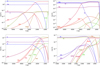 |
Fig. C.1 Benchmark test results of a gas-phase simulation. Light solid lines show GGCHEM output. Dash-dotted lines show our output. Both simulations were run at a constant pressure of p = 10−4 bar, from Τ = 6000 K to Τ = 600 K. The GGCHEM simulation included 120 gas-phase species; our simulation included 40. There were slight differences in the elemental abundance pattern assumed in the two simulations. |
Additionally, we perform a pure gas-phase benchmark test against the open-source condensation code GGCHEM by Woitke et al. (2018), which itself is benchmarked against the open-source gas-phase code TEA by Blecic et al. (2016). In this test, we run both codes ‘as is’, that is, we do not try to make the simulations as similar as possible, but use them in their default configuration, with regards to solar abundance pattern14 and included number of species. We set the disk pressure to the same value in the two simulations and restrict both to the same set of elements.15
The gas-phase benchmark test against GGCHEM shows an overall good agreement (see Fig C.1). The curve shapes are identical for all species included in both simulations, despite the large difference in the total number of included molecules. Most deviations in the relative amounts are explained by differences in the assumed elemental abundance pattern. We consider the found accuracy sufficient for all intended uses of our code.
While the results of the stability tests are all in good agreement, the simulation parameters obviously affect the computation time of the simulation. As shown in Table C.3, the computation time per temperature step is very similar for all test except the lowest resolution of ΔΤ = 10 K. Disregarding this simulation, we find a computation time per temperature step of t = (0.52 ± 0.01) s. Accordingly, the total runtime scales linearly with the number of temperature steps to be calculated.
Comparison of run times for different tests.
Appendix D Included molecule data
Included solid-phase data.
Included gas-phase molecule data.
Included reference state molecule data.
References
- Adibekyan, V. Z., Sousa, S. G., Santos, N. C., et al. 2012, A&A, 545, A32 [NASA ADS] [CrossRef] [EDP Sciences] [Google Scholar]
- Adibekyan, V., Dorn, C., Sousa, S. G., et al. 2021, Science, 374, 330 [NASA ADS] [CrossRef] [Google Scholar]
- Allibert, M., Chatillon, C., Jacob, K. T., & Lourtau, R. 1981, J. Am. Ceramic Soc., 64, 307 [CrossRef] [Google Scholar]
- Asplund, M., Grevesse, N., Sauval, A. J., & Scott, P. 2009, ARA&A, 47, 481 [NASA ADS] [CrossRef] [Google Scholar]
- Atkins, P., & de Paula, J. 2006, Physical Chemistry, 8th edn. (New York: W.H. Freeman & Company) [Google Scholar]
- Ballmer, M. D., & Noack, L. 2021, Elements, 17, 245 [NASA ADS] [CrossRef] [Google Scholar]
- Bedell, M., Meléndez, J., Bean, J. L., et al. 2014, ApJ, 795, 23 [Google Scholar]
- Benz, W., Slattery, W. L., & Cameron, A. G. W. 1988, Icarus, 74, 516 [NASA ADS] [CrossRef] [Google Scholar]
- Bitsch, B., & Battistini, C. 2020, A&A, 633, A10 [NASA ADS] [CrossRef] [EDP Sciences] [Google Scholar]
- Blecic, J., Harrington, J., & Bowman, M. O. 2016, ApJS, 225, 4 [CrossRef] [Google Scholar]
- Bond, J. C., Lauretta, D. S., & O’Brien, D. P. 2010a, Icarus, 205, 321 [NASA ADS] [CrossRef] [Google Scholar]
- Bond, J. C., O’Brien, D. P., & Lauretta, D. S. 2010b, ApJ, 715, 1050 [Google Scholar]
- Bonsor, A., Carter, P. J., Hollands, M., et al. 2020, MNRAS, 492, 2683 [NASA ADS] [CrossRef] [Google Scholar]
- Boyd, S., & Vandenberghe, L. 2004, Convex Optimization (New York, New York, USA: Cambridge University Press), 1 [Google Scholar]
- Brewer, J. M., & Fischer, D. A. 2016, ApJ, 831, 20 [CrossRef] [Google Scholar]
- Brewer, J. M., Fischer, D. A., Valenti, J. A., & Piskunov, N. 2016, ApJS, 225, 32 [Google Scholar]
- Brogi, M., & Line, M. R. 2019, AJ, 157, 114 [Google Scholar]
- Brown, T. M. 2001, ApJ, 553, 1006 [NASA ADS] [CrossRef] [Google Scholar]
- Carlson, R. W., Garnero, E., Harrison, T. M., et al. 2014, Ann. Rev. Earth Planet. Sci., 42, 151 [CrossRef] [Google Scholar]
- Carter-Bond, J. C., O’Brien, D. P., Delgado Mena, E., et al. 2012, ApJ, 747, L2 [NASA ADS] [CrossRef] [Google Scholar]
- Chase, M. W. 1998, Am. Inst. Phys., 1, 1 [Google Scholar]
- Clement, M. S., Raymond, S. N., & Chambers, J. E. 2021, ApJ, 923, L16 [NASA ADS] [CrossRef] [Google Scholar]
- Conn, A. R., Gould, N. I. M., & Toint, P. L. 2000, Trust Region Methods (USA: Society for Industrial and Applied Mathematics) [CrossRef] [Google Scholar]
- Dorn, C., Harrison, J. H. D., Bonsor, A., & Hands, T. O. 2019, MNRAS, 484, 712 [Google Scholar]
- Duncan, M. J., Levison, H. F., & Lee, M. H. 1998, AJ, 116, 2067 [Google Scholar]
- Ebel, D. S., & Grossman, L. 2000, Geochim. Cosmochim. Acta, 64, 339 [NASA ADS] [CrossRef] [Google Scholar]
- Eriksson, G., Lützow Holm, J., Welch, B. J., et al. 1971, Acta Chem. Scandin., 25, 2651 [CrossRef] [Google Scholar]
- Farihi, J., Koester, D., Zuckerman, B., et al. 2016, MNRAS, 463, 3186 [NASA ADS] [CrossRef] [Google Scholar]
- Fegley, Bruce, J. 2000, Space Sci. Rev., 92, 177 [NASA ADS] [CrossRef] [Google Scholar]
- Fortney, J. J. 2012, ApJ, 747, L27 [NASA ADS] [CrossRef] [Google Scholar]
- Fridlund, M., Livingston, J., Gandolfi, D., et al. 2020, MNRAS, 498, 4503 [NASA ADS] [CrossRef] [Google Scholar]
- Fulton, B. J., & Petigura, E. A. 2018, AJ, 156, 264 [Google Scholar]
- Gebek, A., & Matthee, J. 2022, ApJ, 924, 73 [NASA ADS] [CrossRef] [Google Scholar]
- Gu, J. T., Fischer, R. A., Brennan, M. C., et al. 2023, Icarus, 394, 115425 [NASA ADS] [CrossRef] [Google Scholar]
- Harrison, J. H. D., Bonsor, A., & Madhusudhan, N. 2018, MNRAS, 479, 3814 [NASA ADS] [CrossRef] [Google Scholar]
- Hemingway, B., Haas, J., & Robinson, G. 1982, Thermodynamic properties of selected minerals in the system Al2O3-CaO-SiO2-H2O at 298.15 K and 1 bar (10’5 Pascals) pressure and at higher temperatures, Tech Rep. [Google Scholar]
- Herbort, O., Woitke, P., Helling, C., & Zerkle, A. 2020, A&A, 636, A71 [EDP Sciences] [Google Scholar]
- Herbort, O., Woitke, P., Helling, C., & Zerkle, A. L. 2022, A&A, 658, A180 [NASA ADS] [CrossRef] [EDP Sciences] [Google Scholar]
- Hersant, F., Gautier, D., & Huré, J.-M. 2001, ApJ, 554, 391 [NASA ADS] [CrossRef] [Google Scholar]
- Hinkel, N. R., & Unterborn, C. T. 2018, ApJ, 853, 83 [NASA ADS] [CrossRef] [Google Scholar]
- Hinkel, N. R., Young, P. A., Pagano, M. D., et al. 2016, ApJS, 226, 4 [CrossRef] [Google Scholar]
- Izidoro, A., Dasgupta, R., Raymond, S. N., et al. 2022, Nat. Astron., 6, 357 [NASA ADS] [CrossRef] [Google Scholar]
- Johnson, T. V., Mousis, O., Lunine, J. I., & Madhusudhan, N. 2012, ApJ, 757, 192 [NASA ADS] [CrossRef] [Google Scholar]
- Jorge, D. M., Kamp, I. E. E., Waters, L. B. F. M., Woitke, P., & Spaargaren, R. J. 2022, A&A, 660, A85 [NASA ADS] [CrossRef] [EDP Sciences] [Google Scholar]
- Jura, M., & Young, E. D. 2014, Ann. Rev. Earth Planet. Sci., 42, 45 [CrossRef] [Google Scholar]
- Kargel, J. S., & Lewis, J. S. 1993, Icarus, 105, 1 [NASA ADS] [CrossRef] [Google Scholar]
- Keszei, E. 2012 Chemical Thermodynamics (Springer Berlin Heidelberg) [CrossRef] [Google Scholar]
- Khorshid, N., Min, M., Désert, J. M., Woitke, P., & Dominik, C. 2022, A&A, 667, A147 [NASA ADS] [CrossRef] [EDP Sciences] [Google Scholar]
- Kleine, T., Budde, G., Burkhardt, C., et al. 2020, Space Sci. Rev., 216, 55 [CrossRef] [Google Scholar]
- Kley, W. 1999, MNRAS, 303, 696 [NASA ADS] [CrossRef] [Google Scholar]
- Linstrom, P. J., & Mallard, W. G. 1997, NIST Chemistry WebBook, NIST Standard Reference Database 69 [Google Scholar]
- Lodders, K. 2003, ApJ, 591, 1220 [Google Scholar]
- Lodders, K. 2019, ArXiv e-prints [arXiv:1912.00844] [Google Scholar]
- Lodders, K., & Fegley, B. 1993, Earth Planet. Sci. Lett., 117, 125 [CrossRef] [Google Scholar]
- Madhusudhan, N. 2019, ARA&A, 57, 617 [NASA ADS] [CrossRef] [Google Scholar]
- Madhusudhan, N., Piette, A. A. A., & Constantinou, S. 2021, ApJ, 918, 1 [NASA ADS] [CrossRef] [Google Scholar]
- Mollière, P., van Boekel, R., Dullemond, C., Henning, T., & Mordasini, C. 2015, ApJ, 813, 47 [Google Scholar]
- Moriarty, J., Madhusudhan, N., & Fischer, D. 2014, ApJ, 787, 81 [NASA ADS] [CrossRef] [Google Scholar]
- Nissen, P. E. 2013, A&A, 552, A73 [NASA ADS] [CrossRef] [EDP Sciences] [Google Scholar]
- Oberg, N., Kamp, I., Cazaux, S., Woitke, P., & Thi, W. F. 2022, A&A, 667, A95 [NASA ADS] [CrossRef] [EDP Sciences] [Google Scholar]
- O’Brien, D. P., Morbidelli, A., & Levison, H. F. 2006, Icarus, 184, 39 [CrossRef] [Google Scholar]
- Otegi, J. F., Bouchy, F., & Helled, R. 2020a, A&A, 634, A43 [NASA ADS] [CrossRef] [EDP Sciences] [Google Scholar]
- Otegi, J. F., Dorn, C., Helled, R., et al. 2020b, A&A, 640, A135 [NASA ADS] [CrossRef] [EDP Sciences] [Google Scholar]
- Pack, A., Shelley, J. M. G., & Palme, H. 2004, Science, 303, 997 [NASA ADS] [CrossRef] [Google Scholar]
- Petaev, M. I., & Wood, J. A. 1998, Meteor. Planet. Sci., 33, 1123 [NASA ADS] [CrossRef] [Google Scholar]
- Pignatale, F. C., Maddison, S. T., Taquet, V., Brooks, G., & Liffman, K. 2011, MNRAS, 414, 2386 [NASA ADS] [CrossRef] [Google Scholar]
- Pinte, C., Harries, T. J., Min, M., et al. 2009, A&A, 498, 967 [NASA ADS] [CrossRef] [EDP Sciences] [Google Scholar]
- Plotnykov, M., & Valencia, D. 2020, MNRAS, 499, 932 [CrossRef] [Google Scholar]
- Pollack, J. B., Hubickyj, O., Bodenheimer, P., et al. 1996, Icarus, 124, 62 [NASA ADS] [CrossRef] [Google Scholar]
- Portegies Zwart, S. 2020, Nat. Astron., 4, 819 [Google Scholar]
- Pudritz, R. E., Cridland, A. J., & Alessi, M. 2018, in Handbook of Exoplanets, eds. H. J. Deeg, & J. A. Belmonte (Berlin: Springer), 144 [Google Scholar]
- Putirka, K. D., Dorn, C., Hinkel, N. R., & Unterborn, C. T. 2021, Elements, 17, 235 [NASA ADS] [CrossRef] [Google Scholar]
- Raymond, S. N., Quinn, T., & Lunine, J. I. 2004, Icarus, 168, 1 [NASA ADS] [CrossRef] [Google Scholar]
- Righter, K., Drake, M. J., & Scott, E. R. D. 2006, in Meteorites and the Early Solar System II, eds. D. S. Lauretta, & H. Y. McSween (Tucson: University of Arizona Press), 803 [CrossRef] [Google Scholar]
- Robie, R. A., & Hemingway, B. S. 1995, Thermodynamic properties of minerals and related substances at 298.15 K and 1 bar (105 pascals) pressure and at higher temperatures, US Geol. Surv. Bull. 2131 [Google Scholar]
- Robie, R. A., Hemingway, B. S., & Fisher, J. R. 1978, Thermodynamic proper- ties of minerals and related substances at 298.15 K and 1 bar (10’5 pascals) pressure and at higher temperatures, US Geol. Surv. Bull. 1452 [Google Scholar]
- Rodríguez-Mozos, J. M., & Moya, A. 2022, A&A, 661, A101 [NASA ADS] [CrossRef] [EDP Sciences] [Google Scholar]
- Rustamkulov, Z., Sing, D. K., Liu, R., & Wang, A. 2022, ApJ, 928, L7 [CrossRef] [Google Scholar]
- Schneeberger, A., Mousis, O., Aguichine, A., & Lunine, J. I. 2023, A&A, 670, A28 [NASA ADS] [CrossRef] [EDP Sciences] [Google Scholar]
- Schulze, J. G., Wang, J., Johnson, J. A., et al. 2021, Planet. Sci. J., 2, 113 [NASA ADS] [CrossRef] [Google Scholar]
- Seager, S., & Sasselov, D. D. 2000, ApJ, 537, 916 [Google Scholar]
- Sossi, P. A., Stotz, I. L., Jacobson, S. A., Morbidelli, A., & O’Neill, H. S. C. 2022, Nat. Astron., 6, 951 [NASA ADS] [CrossRef] [Google Scholar]
- Souto, D., Cunha, K., García-Hernández, D. A., et al. 2017, ApJ, 835, 239 [Google Scholar]
- Spaargaren, R. J., Ballmer, M. D., Bower, D. J., Dorn, C., & Tackley, P. J. 2020, A&A, 643, A44 [NASA ADS] [CrossRef] [EDP Sciences] [Google Scholar]
- Spaargaren, R. J., Wang, H. S., Mojzsis, S. J., Ballmer, M. D., & Tackley, P. J. 2023, ApJ, 948, 53 [CrossRef] [Google Scholar]
- Teske, J. K., Cunha, K., Smith, V. V., Schuler, S. C., & Griffith, C. A. 2014, ApJ, 788, 39 [CrossRef] [Google Scholar]
- Thiabaud, A., Marboeuf, U., Alibert, Y., et al. 2014, A&A, 562, A27 [NASA ADS] [CrossRef] [EDP Sciences] [Google Scholar]
- Thiabaud, A., Marboeuf, U., Alibert, Y., Leya, I., & Mezger, K. 2015, A&A, 580, A30 [NASA ADS] [CrossRef] [EDP Sciences] [Google Scholar]
- Toppani, A., Libourel, G., Robert, F., & Ghanbaja, J. 2006, Geochim. Cosmochim. Acta, 70, 5035 [NASA ADS] [CrossRef] [Google Scholar]
- Turnbull, M. C. 2015, ArXiv e-prints [arXiv:1510.01731] [Google Scholar]
- Veras, D. 2021, in Oxford Research Encyclopedia of Planetary Science (UK: Oxford University Press), 1 [Google Scholar]
- Wang, H. S., Lineweaver, C. H., & Ireland, T. R. 2019a, Icarus, 328, 287 [NASA ADS] [CrossRef] [Google Scholar]
- Wang, H. S., Liu, F., Ireland, T. R., et al. 2019b, MNRAS, 482, 2222 [NASA ADS] [CrossRef] [Google Scholar]
- White, W. B., Johnson, S. M., & Dantzig, G. B. 1958, J. Chem. Phys., 28, 751 [Google Scholar]
- Wilson, T. G., Farihi, J., Gänsicke, B. T., & Swan, A. 2019, MNRAS, 487, 133 [CrossRef] [Google Scholar]
- Woitke, P., Kamp, I., & Thi, W. F. 2009, A&A, 501, 383 [NASA ADS] [CrossRef] [EDP Sciences] [Google Scholar]
- Woitke, P., Helling, C., Hunter, G. H., et al. 2018, A&A, 614, A1 [NASA ADS] [CrossRef] [EDP Sciences] [Google Scholar]
- Wood, J. A., & Hashimoto, A. 1993, Geochim. Cosmochim. Acta, 57, 2377 [NASA ADS] [CrossRef] [Google Scholar]
- Wood, B. J., Smythe, D. J., & Harrison, T. 2019, Am. Mineral., 104, 844 [NASA ADS] [CrossRef] [Google Scholar]
- Worters, M., Millard, D., Hunter, G., Helling, C., & Woitke, P. 2018, Comparison Catalogue of Gas-Equilibrium Constants, Kp, University of St Andrews [Google Scholar]
- Xu, S., & Bonsor, A. 2021, Elements, 17, 241 [NASA ADS] [CrossRef] [Google Scholar]
- Zeng, L., Jacobsen, S. B., Sasselov, D. D., et al. 2019, Proc. Natl. Acad. Sci., 116, 9723 [Google Scholar]
- Zimmer, K., Zhang, Y., Lu, P., et al. 2016, Comput. Geosci., 90, 97 [NASA ADS] [CrossRef] [Google Scholar]
Equilibrium Condensation & Composition Of planets, or in Italian roughly ‘There you have it: planets’. Available at https://github.com/AninaTimmermann/ECCOplanets
This is a slight deviation from the definition of the constants in the NIST-JANAF web-book (Linstrom & Mallard 1997).
We acknowledge the fact that Python is not a particularly efficient coding language (see our performance test in Table C.3 and compare to e.g. Woitke et al. (2018), who use Fortran-90 in their GGCHEM-code), and understand the growing concern about the ecological impact of computational astrophysics (Portegies Zwart 2020). Our choice is motivated by the conjecture that Python is most commonly taught and used in physics, astronomy, and geosciences, and our aim to also make our code accessible to an audience with limited coding experience.
The deviation of the Fe condensation temperatures at low metallicities is caused by the superposition of the effect of disproportionately low Fe-abundances in the stellar sample (‘α-enhancemenť; see e.g. Gebek & Matthee 2022).
The Hersant et al. (2001) disk profile is not considered state-of-the-art anymore, as it is a purely diffusive model. It has been shown that introducing radiative transfer to the model inverses the vertical temperature profile of the disk (i.e. T increases for increasing z) compared to a purely diffusive model in which the temperature decreases with distance from the midplane, and a shadowing effect results in an overall cooler mid-plane (Pinte et al. 2009; Woitke et al. 2009; Oberg et al. 2022). However, for the purpose of our analysis, the only essential aspect of the diskprofile is that the midplane temperature decreases with distance from the star.
The GGCHEM code (Woitke et al. 2018), on the other hand, contains thermochemical data of 12 different solid S species.
GGCHEM uses the solar abundance pattern as reported by Asplund et al. (2009).
All Tables
Summary of the influence of the variation in different element ratios on the condensation temperature of elements.
50% condensation temperature of different elements for variations in the T parameter.
Elemental composition of solids at different temperatures as a function of variations in the T parameter.
All Figures
|
Fig. 1 Example of graphical output of the molecule database for corundum (A12O3(s)). Top panel: Entropy. Middle panel: Enthalpy. Bottom panel: Gibbs energy (chemical potential). Blue diamonds show tabulated values (upper two panels) and solid black lines the corresponding fitted Shomate function. |
| In the text | |
|
Fig. 2 Example of the progression of solid species of a simulation. The molar amount relative to the total molar content of the disk of each of the condensates included in the simulation is shown as a function of decreasing temperature in different line colours and styles, as denoted in the legend. See Appendix D for details on the included species. The simulation was run at a constant disk pressure of p = 10−4 bar and is based the solar elemental abundance pattern recommended by Lodders (2003). See Table B.2 for a summary of the simulation parameters. |
| In the text | |
|
Fig. 3 Example of the condensation curve and condensation temperature of a specific element, here Ca. The dark blue curve shows the fraction of Ca atoms bound in gas-phase species, the blue line shows the fraction of Ca atoms bound in solid-phase species. The T-value of the intersection at 50% of atoms in gas- and solid-phase signifies the 50% condensation temperature. |
| In the text | |
|
Fig. 4 Examples of different types of condensation behaviours of solid species. We show the relative molar amount of the species present in the protoplanetary disk as a function of decreasing temperature to demonstrate our definition of 50% condensation temperatures. Red diamonds show the computed 50% condensation temperatures. Left panel: progression of perovskite CaTiO3(s) (condensation and subsequent disintegration). Right panel: progression of forsterite Mg2SiO4(s) (varying relative amounts). |
| In the text | |
|
Fig. 5 Graphical comparison of deviation of 50% condensation temperatures of the major rock-forming elements, minus the mean over the three values for each element. |
| In the text | |
|
Fig. 6 Dependence of the 50% condensation temperature (Tc) of elements on the disk pressure. Markers represent simulated condensation temperatures, and corresponding dashed lines are only to guide the eye. Colours, as denoted in the legend, are the same for both panels. All simulations use the solar elemental abundance pattern recommended by Lodders (2003). Top panel: 50% condensation temperature of major planet-building elements as a function of different disk pressures. Bottom panel: deviation of the 50% condensation temperature from the respective mean condensation temperature. |
| In the text | |
|
Fig. 7 Parameter range of the Brewer et al. (2016) stellar database. Grey background markers represent all stars with logɡ > 3.5 and S/N > 100 of the database, and light blue foreground markers represent the stellar sample studied here. Left panel: effective temperature versus metallicity. Middle panel: C/O ratio versus Al/Ca ratio. Right panel: Mg/Si ratio versus Fe/O ratio. |
| In the text | |
|
Fig. 8 Correlation between the C/O and Σ/Ο, where Σ = NMg + NSi + NFe, + NCa + NAl. Grey background markers represent the studied stellar sample, and the dotted line shows the fit quadratic fit to the data. The light blue foreground markers show the synthetic data for the C/O analysis. |
| In the text | |
|
Fig. 9 Correlation between the overall metallicity of the system and the condensation temperature of some major planet-building elements. The coloured circles in the foreground show the simulation results of the synthetic abundance patterns, and the grey circles in the background show the simulation results of a representative subset of approximately 100 stars from the Brewer et al. (2016) database. All simulations were run at a constant disk pressure of p = 10−4 bar. |
| In the text | |
|
Fig. 10 Correlation between the C/O ratio and the condensation temperature of some major planet-building elements, corrected for the metallicity effect. The coloured circles in the foreground show the simulation results of the synthetic abundance patterns, and the grey circles in the background show the simulation results of a representative subset of approximately 100 stars from the Brewer et al. (2016) database. All simulations were run at a constant disk pressure of p = 10−4 bar. |
| In the text | |
|
Fig. 11 Correlation between element ratios and the condensation temperatures, corrected for the metallicity and C/O effect. The coloured circles in the foreground show the simulation results of the synthetic abundance patterns, and the grey circles in the background show the simulation results of a representative subset of approximately 100 stars from the Brewer et al. (2016) database. All simulations were run at a constant disk pressure of p = 10−4 bar. Left panel: influence of the Al/Ca ratio on the condensation temperature of Al and Ca. Right panel: influence of the Mg/Si ratio on the condensation temperature of Mg and Si. |
| In the text | |
|
Fig. 12 Illustration of the three different FZ models for creating a planet’s composition at a given temperature. The x-axis denotes the temperature, or equivalently the distance from the star. Top panel: Gaussian profile. Middle panel: Boxcar profile. Bottom panel: No FZ model. |
| In the text | |
|
Fig. 13 Predicted bulk composition (in wt – %) of a rocky planet simulated for the elemental abundance of HD 27442 (low carbon system). Top panel: B10 planet composition results from four separate simulation runs. We also show our simulations: with a Gaussian FZ (second panel), a boxcar FZ (third panel), and no FZ (bottom panel). The arrows between the first two panels indicate roughly the location of the best correspondence between the Bond simulation and ours. |
| In the text | |
|
Fig. 14 Predicted bulk composition (in wt-%) of a rocky planet simulated for the elemental abundance of HD 17051 (medium carbon system). Top panel: B10 planet composition results from four separate simulation runs. We also show our simulation: with a Gaussian FZ (second panel), with a boxcar FZ (third panel), and with no FZ (bottom panel). The arrows between the first two panels indicate roughly the location of the best correspondence between the Bond simulation and ours. |
| In the text | |
|
Fig. 15 Predicted bulk composition (in wt-%) of a rocky planet simulated for the elemental abundance of HD 17051 (high carbon system). Top panel: B10 planet composition results from four separate simulation runs. We also show our simulation with a Gaussian FZ (second panel), with a boxcar FZ (third panel), and with no FZ (bottom panel). The arrows between the first two panels indicate roughly the location of the best correspondence between the Bond simulation and ours. |
| In the text | |
|
Fig. C.1 Benchmark test results of a gas-phase simulation. Light solid lines show GGCHEM output. Dash-dotted lines show our output. Both simulations were run at a constant pressure of p = 10−4 bar, from Τ = 6000 K to Τ = 600 K. The GGCHEM simulation included 120 gas-phase species; our simulation included 40. There were slight differences in the elemental abundance pattern assumed in the two simulations. |
| In the text | |
Current usage metrics show cumulative count of Article Views (full-text article views including HTML views, PDF and ePub downloads, according to the available data) and Abstracts Views on Vision4Press platform.
Data correspond to usage on the plateform after 2015. The current usage metrics is available 48-96 hours after online publication and is updated daily on week days.
Initial download of the metrics may take a while.