| Issue |
A&A
Volume 694, February 2025
|
|
|---|---|---|
| Article Number | A303 | |
| Number of page(s) | 21 | |
| Section | Planets, planetary systems, and small bodies | |
| DOI | https://doi.org/10.1051/0004-6361/202451070 | |
| Published online | 21 February 2025 | |
The compositional diversity of rocky exoplanets around K-dwarf stars
1
Centre for Planetary Habitability (PHAB), Department of Geosciences, University of Oslo,
PO Box 1028
Blindern,
0315
Oslo,
Norway
2
Department of Earth Sciences, University College London,
Gower Street,
London
WC1E 6BT,
United Kingdom
3
Konkoly Observatory, HUN-REN CSFK, MTA Centre of Excellence ;
Konkoly Thege Miklos St. 15–17,
1121
Budapest,
Hungary
★ Corresponding author; petra.hatalova@geo.uio.no
Received:
11
June
2024
Accepted:
16
December
2024
Context. The mass-radius distribution of currently known exoplanets suggests a fascinating variety in terms of their chemical compositions. Still, the interior structures and compositions of rocky exoplanets are essentially inaccessible to observations. Here, we present a model that combines planet formation simulations with equilibrium condensation models to estimate the interior composition and structure of exoplanets around K-dwarf stars.
Aims. In a previous study, we reproduced the observed population of close-in super-Earths around K-dwarf stars with suitable initial conditions. However, the masses and radii of these simulated planets are not self-consistent, since the radius information is postprocessed based on an assumed constant average density (3 g cm−3). In this work, we have incorporated compositions into the N-body simulations using the chemistry of the protoplanetary disk from equilibrium condensation sequences, together with thermodynamics of the various mineral phases. This has allowed us to develop models of likely interior structures, bulk densities, and, thus, radii for rocky exoplanets.
Methods. We selected the outcomes of ten N-body simulations around a 0.8 M⊙ star that best reproduced the observed population. We employed stellar abundances from six K-dwarf stars with a range of metallicities. Based on the condensation sequence and the temperature-pressure profile of a disk, we assigned bulk elemental compositions to planetesimals and then tracked materials accreted onto planets during their formation.
Results. We have obtained a set of planets with more realistic radii determinations than those purely based on one preset density for all bodies. We formed various types of planets: i) Ca- and Al-rich(er), ii) Mg-depleted, iii) fully oxidized core-less planets, iv) planets similar to Earth or Mars in composition and core size, and v) planets with different core mass fractions (from significantly smaller than the Martian core to significantly larger than the Earth’s core); however, we do not have Mercury-like planet with a huge core.
Key words: planets and satellites: composition / planets and satellites: formation / planets and satellites: interiors
© The Authors 2025
 Open Access article, published by EDP Sciences, under the terms of the Creative Commons Attribution License (https://creativecommons.org/licenses/by/4.0), which permits unrestricted use, distribution, and reproduction in any medium, provided the original work is properly cited.
This article is published in open access under the Subscribe to Open model. Subscribe to A&A to support open access publication.
1 Introduction
One of the main goals in the detection and characterization of exoplanets is to recognize rocky exoplanets that are similar to Earth in size and mass and that are potentially even habitable. This is a difficult task as the stability of Earth’s environment, crucial for sustaining life, is determined by the planet’s bulk composition, internal structure, and dynamic processes (Shahar et al. 2019; Van Hoolst et al. 2019), all of which are currently inaccessible to our observations. Previous studies used mass–radius models to estimate the composition of small exoplanets by comparing a planet’s measured density to the density predicted by interior models with the mass/radius as input (e.g., Seager et al. 2007; Valencia et al. 2007; Howard et al. 2013; Dressing et al. 2015; Dorn et al. 2015; Unterborn et al. 2016; Zeng et al. 2016,2019). However, it has been shown that multiple different compositions are capable of producing the same total mass and radius (Seager et al. 2007), so that only an approximate planetary composition can be determined from mass and radius measurements alone, as the problem is highly underconstrained (Rogers & Seager 2010). The stellar elemental abundances of the host stars have been added as another important constraint. To first order, the stars can be used as proxies of planetary abundances, at least for refractory elements, because stars and planets are made of the same material from the stellar nebulae. Exoplanetary bulk compositions of the major planet-building elements Mg, Si, Al, Ca, and Fe are often assumed to match the host star abundances exactly (e.g., Dorn et al. 2015; Thiabaud et al. 2015; Unterborn et al. 2016).
However, to make better estimates, we also need also to consider the devolatilization process that actually produces the rocky planets from the nebulae. The differences in the elemental abundances of volatiles in the Sun versus the abundances in the Earth and chondritic meteorites, which appear to be most representative of the material that formed the Earth, can be explained by the different condensation temperatures of the various volatile elements (Lodders 2003). This implies that we can estimate where planetary bodies formed in a disk by analyzing the depletion in the abundances of certain species with respect to the host star’s abundances. Wang et al. (2019a) quantified the devolatilization pattern for the Earth based on a combination of solar photospheric abundances and CI chondritic abundances. Their study established a devolatilization factor of 10–20% for the main planet-building elements of rocky planets such as Si, Mg, Fe, and Ni; whereas elements like O, S, and C could be devolatilized by more than 80–90%. Additionally, Sossi et al. (2022) has proposed that the Earth did not form only from chondrites, but by the stochastic accretion of numerous precursor bodies, each with its own varying composition reflecting the temperatures during their formation. We could argue that the depletion of volatiles is not exclusive to our Solar System and should be expected to be a common occurrence during the formation of rocky planets, both within and beyond our planetary system. Devolatilized host stellar abundances have been already used in several studies, albeit only for the so-called “exo-Earths” or habitable-zone terrestrial exoplanets (Wang et al. 2019b, 2022a,b); this is because the employed devolatilization pattern was determined for the Earth (Wang et al. 2019a) and it remains uncertain to what extent it can be applied more broadly to exoplanets.
The increasingly accurate measurements of planetary masses and radii (e.g., Weiss et al. 2016; Stassun et al. 2017; Fulton et al. 2017; Fulton & Petigura 2018; Fridlund et al. 2020; Otegi et al. 2020), together with high-precision stellar abundances of the elements obtained from stellar photospheres (e.g., Nissen 2015; Brewer & Fischer 2016; Brewer et al. 2016; Liu et al. 2015; Delgado Mena et al. 2017; Bedell et al. 2018; Adibekyan et al. 2021) have been used in various models that predict interior structure and/or composition of exoplanets or their building blocks (e.g. Bond et al. 2010b; Carter-Bond et al. 2012b; Thiabaud et al. 2014; Dorn et al. 2019; Bitsch & Battistini 2020; Wang et al. 2022b; Unterborn et al. 2023). Additionally, as planet composition is inherently tied to its formation (e.g., Bond et al. 2006,2010b; Elkins-Tanton & Seager 2008; Thiabaud et al. 2015; Dorn et al. 2015; Unterborn et al. 2018), obtaining a better understanding of the formation of the Solar System and other planetary systems is crucial. This can be achieved, for example, by studying chondrites, along with the specific processes that occurred in the primordial planet-building material (e.g., Ireland & Fegley Jr 2000; Kwok 2016; Norris & Wood 2017), or via planet formation simulations (e.g., Raymond et al. 2007; Brasser et al. 2016a,b; Izidoro et al. 2017; Raymond et al. 2018; Miguel et al. 2020; Woo et al. 2022; Hatalova et al. 2023).
The interiors of rocky exoplanets may remain largely inaccessible for our telescopes. After all, our current knowledge of the bulk chemical compositions of planets in our own system, including the Earth, is still limited, even though it has been immensely expanded during the last decades (e.g., McDonough & Sun 1995; Ireland & Fegley Jr 2000; McDonough 2003; Palme & Zipfel 2017; Yoshizaki & McDonough 2020; McDonough & Yoshizaki 2021; Khan et al. 2022). Currently, the most direct technique providing information about the composition of exoplanetary building blocks is the spectroscopic analysis of polluted white dwarfs exhibiting heavy elements such as Mg, Fe, and Ca in their atmospheres (e.g., Jura & Young 2014; Farihi et al. 2016; Harrison et al. 2018; Wilson et al. 2019; Bonsor et al. 2020). However, observations and characterizations of exoplanets and their atmospheres with the James Webb Space Telescope (JWST; Morley et al. 2017; Gialluca et al. 2021), as well as other, mostly space-based missions such as Ariel (Tinetti et al. 2018; Turrini et al. 2022) or PLATO (Rauer et al. 2014; Nascimbeni et al. 2022), will certainly reveal new details of the surface and interior characteristics of rocky exoplanets.
In this work, we focus on close-in super-Earths orbiting K-dwarf stars. K dwarfs are main-sequence stars with masses and radii a bit smaller than our Sun, which are of particular interest in the search for extraterrestrial life (e.g., Arney 2019). It has been estimated that at least 30–50% of the FGK spectral-type stars host super-Earths with orbital periods shorter than 100 days (e.g., Mayor et al. 2011; Howard et al. 2012; Fressin et al. 2013; Mulders et al. 2018), so they make up one of the largest populations of known exoplanets. The distribution of observed exoplanets on the mass-radius diagram indicates a fascinating diversity in their bulk chemical compositions (Fortney et al. 2007; Howard et al. 2013). This gives rise to several factors, including differences in the metallicities of their host stars or the accretion of material at different locations in disks surrounding young stars with similar compositions. Planets form in a compositional gradient dictated by thermodynamic equilibrium in the protoplanetary disk and the chemical composition and temperature of the young central star (Berg et al. 2009). In order to constrain the bulk compositions and interior structures of the planets, we have built upon our previous study (Hatalova et al. 2023), where we reproduced the observed exoplanetary systems (often containing multiple super-Earths) around this type of star. On the basis of dynamical simulations, the resulting planets could be characterized only by mass, with an assigned average density for the apparent radius. Here, we implement the composition for deriving a planet’s density and, consequently, its corresponding radius. Depending on the appropriate core mantle fraction, the compression has a variable impact on the final radius of a planet.
First, we implemented equilibrium condensation simulations for rocky planets produced from stellar abundances using the ECCOplanets code (Timmermann et al. 2023) into our initial bodies (planetesimals and planetary embryos) based on a chosen protoplanetary disk model (Chambers 2009). We also used the database of thermochemical data and the database of stellar abundance patterns included in the code. Afterward, we tracked the dynamical evolution of our planetary bodies for 100 million years, which allowed us to predict the final bulk composition of each of the planets in an ensemble of different possible planetary systems. We then used ExoPlex code (Unterborn et al. 2023) to calculate a planet’s radius, density, core mass fraction, and interior composition from its simulated bulk elemental composition and mass.
This paper is structured as follows. In Sect. 2, we introduce our sample of the simulated planetary systems, and describe the protoplanetary disk model we applied, together with stellar abundances and the employed equilibrium chemistry condensation model. In Sect. 3, we present the results of simulated systems with their predicted chemical compositions and interior structures. In Sect. 4, we discuss our model and results, along with their significance and implications. Finally, in the last section we present the main conclusions of our study.
2 Methods
2.1 Planet formation simulations
The sample of simulated planetary systems used in this study was published in Hatalova et al. (2023). The N-body simulations were run using the GENGA software (Grimm & Stadel 2014; Grimm et al. 2022), which is a a GPU implementation of a hybrid symplectic N-body integrator for simulating planetary dynamics in the final stages of planet formation, and the evolution of planetary systems. Each simulation began with 12 000 bodies with radii of between 200 and 2000 km, and initial locations between 0.2 to 2 AU from the star. Our model included mass growth by planetesimal accretion and mergers (no fragmentation), type-I migration, and eccentricity and inclination dampening from gas drag. We followed the dynamical evolution of the planetary bodies for 100 million years, and tracked the initial locations of the planetesimals and planetary embryos, the mergers, and the locations of the planets they ended up in.
For this study, we specifically selected the outcomes of ten simulations around a star with a mass of 0.8 M⊙ (see Fig. 1) that best reproduce the currently known population of planets observed around K-dwarf stars and their system characteristics. Table 1 presents the main input parameters, specifically the variations in dynamical parameters, corresponding to the ten selected sets of simulation outcomes. All other input parameters remain fixed. As illustrated in Fig. 1, the increasing initial disk mass (or the solid surface density) with the simulation number typically produces more massive inner planets. On the other hand, the variations in gas surface density do not result in any significant differences in the simulation outcomes. The formation, evolution, and main characteristics of these systems are documented in detail in Hatalova et al. (2023).
The observed population consists of 46 multi-planet systems retrieved from the NASA Exoplanet Archive1 in January 2024. The systems contain at least two planets each and there are 139 planets in total (only planets with known masses are considered). A typical known K-dwarf planetary system does not contain giant planets, but it comprises (on average) three planets, mostly super-Earths or sub-Neptunes with very short semimajor axes (typically shorter than the semimajor axis of Mercury). This characteristic is in large part due to observational biases. It is very likely that at least some of the systems in the retrieved sample are not complete, as suggested by studies of completeness of Kepler systems (e.g., Petigura et al. 2013; Zink et al. 2019; Bryson et al. 2020).
Our simulated sample, in accordance with the observed population, does not contain giant planets and our systems typically contain more planets than the known systems. The individual simulations were started with slightly different initial disk masses and gas and planetesimal surface densities to explore the diversity of possible terrestrial planets around this type of star. The sample includes 10 planetary systems with 70 planets together, from 5 to 9 planets per system, with masses between 0.5 and ~12 M⊕, and semimajor axes approximately between 0.06 and 1.8 AU. We excluded all planets with masses above 7 M⊕ from the original sample for some of the analyses because those would have probably accreted substantial amounts of gas during their formation, however, the model used in Hatalova et al. (2023) did not include gas accretion.
Main dynamical input parameters of the selected simulation outcomes.
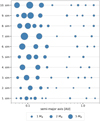 |
Fig. 1 Outcomes of ten planet formation simulations around a 0.8 M⊙ star (Hatalova et al. 2023) that best reproduce the currently known population of planets observed around K-dwarf stars and their system characteristics, after 100 million years of dynamical evolution. |
All possible gaseous (top) and solid (bottom) species.
2.2 Stellar abundances and equilibrium condensation simulations
The chemical conditions in our disk were computed using the ECCOplanets code (Timmermann et al. 2023). The code calculates 50% condensation temperatures of the most common planet-building rocky species based on Gibbs energy minimization. The calculated condensation temperature values are in an excellent agreement with the other commonly used condensation temperatures (Lodders 2003; Wood et al. 2019). All the possible gaseous and solid species that could form in our equilibrium condensation simulations are listed in Table 2. Although the list is limited, these elements and molecular species are the most abundant in the rocky debris of the Solar System, and we assume that the list is sufficient because the stellar sample used in this study is not that different compared to the Sun, as will be demonstrated in Sect. 2.4 and 3.1. Our list of possible species is nearly identical to that used in Dorn et al. (2019) for K- and G-dwarf stars, with the exception of a few species that are not included in the ECCOplanets code. Figure 2 shows the condensation sequences for Kepler-94 and Kepler-62, where the dust species from Table 2 condense out of the disk. Based on the sequences, the predicted elemental bulk compositions of the planetary bodies formed at different temperatures (for the same star) and are presented in Fig. 3. The disk pressure in these equilibrium condensation simulations is 4.2 × 10⁻⁴ bar (constant throughout the disk). For the simulations in this work, the pressure was chosen in accordance with the disk profile described in the next subsection. For comparison, the value usually assumed for the formation of the Earth is 10−4 bar (Fegley 2000; Lodders 2003; Wood et al. 2019).
As discussed in Sect. 1, a devolatilization process needs to be taken into account when using the host star’s composition as a proxy for planet composition. In the ECCOplanets code, the devolatilization pattern is connected to the condensation temperatures of the elements; that is, if an element has not (fully) condensed at a certain temperature, it will automatically be relatively depleted compared to the host star. This approach is similar to the one reported in Sossi et al. (2022).
We use stellar abundance measurements from Brewer et al. (2016). Specifically, we have used abundances from six smaller K-dwarf stars with a range of metallicities ([M/H] = −0.33 to +0.33 dex) and reported values for all the 10 major rock-forming elements: Mg, Si, Fe, Ni, Al, Ca, Na, O, C, and S. Sulfur is actually not reported in Brewer et al. (2016), probably because it is difficult to measure, particularly for the smaller stars such as K and M dwarfs. Cooler stars have more complex molecular spectra and the known sulfur lines become very weak at lower temperatures (Silva et al. 2020). However, as [S/H] and [Fe/H] are well correlated for smaller stars, we estimated the S abundances for our stars based on their measured [Fe/H] values. The [S/H]-[Fe/H] correlation plot is included in Appendix A. We used [Fe/H] for the scaling instead of, for example, [Si/H] that has been well shown in the observations (e.g., Chen et al. 2002). This was because we employed the database of stellar abundances included in the ECCOplanets code (Timmermann et al. 2023), and the code only considers relative amounts of species, with all molar amounts specified relative to an initial abundance of 106 Si atoms. Also, during nucleosynthesis, iron primarily comes from silicon burning, albeit indirectly. Silicon burning leads to the creation of nickel, which then decays into iron, establishing a nucleosynthetic correlation between Si and Fe. Nevertheless, for stars with C/O ratio below 0.8, which are all the stars used in this work (see Sect. 3.1), S species are not expected to play a major role in the equilibrium chemistry (Timmermann et al. 2023), at the temperature range relevant to this study.
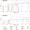 |
Fig. 2 Condensation sequences of all possible solid species (Table 2) in the equilibrium condensation simulations for Kepler-94 (the most metalrich) and Kepler-62 (the most metal-poor) stars computed using ECCOplanets code (Timmermann et al. 2023). The molar amount relative to the total molar content in the disk for each of the condensates is displayed as a function of decreasing disk temperature at a constant disk pressure of 4.2 × 10⁻⁴ bar. Stellar abundances are from Brewer et al. (2016), with S abundances estimated based on [Fe/H] values. |
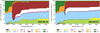 |
Fig. 3 Predicted bulk compositions (in wt%) of rocky planetary bodies as a function of temperature based on the condensation sequences computed using ECCOplanets code (Timmermann et al. 2023) for Kepler-94 metal-rich and Kepler-62 metal-poor stars (see Fig. 2). Stellar abundances are from Brewer et al. (2016), with S abundances estimated based on [Fe/H] values. |
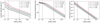 |
Fig. 4 Radial profiles of surface density, mid-plane temperature, and pressure at various times throughout the evolution of the protoplanetary disk. The dashed brown lines at 0.2 and 2 AU illustrate the range of initial locations of planetesimals in our disk. The disk model is described in detail in Appendix B and its parameters are outlined in the text. |
2.3 Temperature–pressure profile of the protoplanetary disk
To determine the temperature as a function of distance from the star, we employed the temperature profile from the commonly used protoplanetary disk model of Chambers (2009), which describes a viscously heated and irradiated disk. The model was also used to calculate the surface density as a function of the distance and, on that basis, the pressure profile of the disk as well. Chambers (2009) divided the disk into three regions according to what is the main source of heating at that distance from the star: an inner viscous evaporating region, intermediate viscous region, and outer irradiated region. The transition radii between the individual regions move inwards as the disk cools down. As we focus particularly on the inner part of a very young disk, only the two first regions are important for us. The model and all the necessary analytical expressions are described in detail in Appendix B. As it is a simple model, such processes as vertical or radial mixing, which may be very important in a real disk, are not considered and all the calculated values are mid-plane values. This limitation is partially compensated by integrating the model into our dynamical simulations.
The radial profiles of surface density, mid-plane temperature and pressure at various times throughout the evolution of the protoplanetary disk are presented in Fig. 4. We used the following disk parameters to compute the profiles: the initial radial extent of the disk, s0 = 33 AU; its initial solid (dust) mass, M0 = 0.1 M*; the opacity, κ0 = 3 cm2 g−1; and M*, R*, and T* (see Table 3), which are the mass, radius, and temperature of the star. The viscosity alpha parameter is α = 0.001, which is a commonly assumed value used in similar studies. Other parameters are introduced in Appendix B. Utilizing these values corresponds to the second example in Stepinski (1998), which is consistent with a planetesimal-forming disk around a solar mass star, with some of the values modified to reflect a typical K-dwarf star. The disk mass of 0.1 M* can be determined by employing the commonly used 1:100 dust-to-gas ratio in a disk (Bohlin et al. 1978) and the following relation:
 (1)
(1)
where 0.2 to 33 AU represent the initial radial extent of the disk, while Σsolid is the solid surface density taken from the planet formation simulations in Hatalova et al. (2023).
As the pressure and temperature in the disk are a function of time and the radial location, so is the composition of the initial bodies. In our model, the planetesimals formed at the distances between 0.2 and 2 AU from the star under conditions at a specific time since the formation of the disk. Since according to the condensation sequences in Fig. 2, the first solids in the disk formed at temperatures of approximately 1650 K, we chose the location corresponding to this temperature as the location of the closest planetesimal (at 0.2 AU) from the star. This way we determined that a planetesimal formation time of t = 0.2 megayears (Myr) or later is reasonable for our model. At earlier formation times, there would be no solids available to form the planetesimals closest to the star due to very high temperature. For example, Bond et al. (2010a) found that using disk conditions obtained for t = 0.5 Myr gave the best fit for the compositions of Venus, Earth, and Mars, and therefore for the formation time of the building blocks for the rocky planets in the Solar System. Alternatively, according to Matsumura et al. (2016) the formation time of approximately t = 0.2 Myr is most preferable for the Solar System using a comparable methodology. In addition, multiple Solar System studies have shown that planetesimals formed rapidly within the first megayear (Halliday & Kleine 2006; Kruijer et al. 2014; Schiller et al. 2015; Morbidelli et al. 2022; Sossi et al. 2022). A planet-sized body probably accumulated material from a range of formation locations and times, primarily due to orbital migration. In this study, the formation location range covers almost 2 AU, as planetary building blocks are sourced from throughout the disk, and we assume that all building blocks in a system formed at the same time.
One of the key properties of a protoplanetary disk is the location of the snow line, which determines the potential water content of rocky planets, particularly in the habitable zone. It is usually defined as the point where the temperature T = 160 K (Min et al. 2011). The temperature range in the part of our disk where the planetesimals are located initially is approximately between 1650–1500 K and 350–250 K, depending on the simulation and the planetesimal formation time (the later the formation, the cooler the disk). Additionally, the condensation sequence model can generate bulk composition estimates down to 300 K (the lowest limit, see Fig. 3). Therefore, the location of the snow line is beyond the edge of the planetesimal disk, and the planetary building blocks are assumed to be quite dry. The temperature range, together with the edge of the planetesimal disk, could be extended in a future study in order to explore the potential water content of the simulated planets.
Stellar physical parameters.
2.4 Chemical composition of planetesimals and final planets
To model the bulk compositions of the initial bodies in our N-body simulations, we employed a simple assumption that rocky planets form via aggregation of rocky planetesimals that have condensed out of a protoplanetary disk in a chemical equilibrium. This model has been demonstrated to reproduce, to first order, the bulk compositions of the terrestrial Solar System bodies (Moriarty et al. 2014; Harrison et al. 2018), and it has been also used to estimate the elemental bulk compositions of rocky exoplanets (Bond et al. 2010b; Carter-Bond et al. 2012b). The initial elemental composition of the disk was assumed to be identical to the undevolatilized stellar nebula, but the elemental compositions of the planetesimals were computed from the devolatilized stellar nebula (i.e., the fraction of condensates relative to the initial stellar nebula) based on their “formation temperature. This is the temperature at which the planetary material decouples from the chemical equilibrium of the disk, corresponding to their initial distance from the star. Basically, we assigned each planetesimal (or planetary embryo) its elemental composition based on where they formed in the disk as displayed in Fig. 3. From the figure, it is evident that planetesimals that formed at very high temperatures (> 1200 K) will have significantly different compositions compared to the bodies formed at lower temperatures, where most solids are condensed out. At the lower temperatures, the differences between the assigned compositions are generally smaller. When the planetesimals fall outside the lower limit, they are assigned the formation temperature of 300 K. Figure 3 presents two examples of stars with very different metallicities, demonstrating that varying stellar abundances are expected to result in different bulk compositions. We chose six smaller stars with stellar abundances (see Table 4) and various metallicities (see Table 3) for this study.
The elemental bulk compositions of the final simulated planets are the sum of each object that they accreted. Phase changes and outgassing were not considered, and all collisions were assumed to lead to perfect accretion, meaning no fragmentation or mass loss occurred, and all buildings blocks contributed equally with their compositions to the bulk composition of the final rocky planet.
The next step was to calculate the equilibrium interior composition (i.e., mantle oxide composition and core composition) of the planets based on their elemental compositions. For that purpose, we utilized the ExoPlex code (Unterborn et al. 2023), which allows us to determine a planet’s radius, density, core mass fraction, and the mantle and core chemistry from its bulk composition and mass. However, as the mass fraction of FeO in a mantle is a free parameter, we first estimated its value for our planets. This was done by balancing all the available oxygen in a planet with all the available cations, such as Mg, Si, Al, Na, etc., to produce oxides in the mantle following an oxidation sequence. The remaining oxygen then formed FeO. The left over Fe was assumed to be in the core. A few different oxidation sequences of major elements have been used in recent studies. SiO2–CaO–Na2O–MgO–Al2O3–FeO–NiO–SO3 was applied in Wang et al. (2019b) and later modified by Wang et al. (2022b) to Na2O–CaO–MgO–Al2O3–SiO2–FeO– NiO–SO3–CO2–C(graphite/diamond)-metals. The modification was implemented to allow for the potential partial oxidation of Si in case of a reduced mantle, as Si can be an important light element occurring it metallic cores (McDonough 2003; Hirose et al. 2013; Li & Fei 2014; Wang et al. 2018). We employed the oxidation sequence as described in Wang et al. (2022b), and then found solutions for a two-layer model of our planets consisting only of a core and a mantle by running the ExoPlex code.
We also tested the effect of adjusting core chemistry by adding variable amounts of light elements, specifically O, Si and S, to the core. This acts to lower the density of the core, compared to a pure Fe core, and potentially increase its size. The Earth’s core also contains other elements besides Fe (Birch 1952), the most abundant of these elements being Ni at ~5 wt% (McDonough 2003). Additionally, it contains ~8 wt% of lighter elements (e.g., McDonough 2003; Badro et al. 2015; Li et al. 2019). Nevertheless, what exactly these light elements are remains a topic of ongoing debate.
Stellar elemental abundances in differential logarithmic units (dex) from Brewer et al. (2016).
3 Results
3.1 Key stellar geochemical ratios
As noted earlier in this paper, the stellar sample used in this work is based on planet-hosting K-dwarf stars, with masses less than 1 M⊙ and metallicities covering the range from approximately −0.3 to +0.3 dex. Each of the stars has been confirmed to host at least one potential super-Earth with a maximum mass of ~10 M⊕.
The most important stellar elemental ratios to determine the interior composition of a rocky exoplanet are C/O and Mg/Si (the elemental number ratios). If the values of C/O are larger than 0.8, then carbide planets may form around the star (Bond et al. 2010b; Teske et al. 2014; Brewer & Fischer 2016). Nevertheless, this is not the case for any of our stars (see Fig. 5), therefore we did not expect to form planets deviating from the standard silicate chemistry. Additionally, Mg/Si ratio controls the mineralogy in the mantle of a silicate planet. If Mg/Si < 1, pyroxene (MgSiO3) and various silicate species, such as feldspars, should be the dominant mineral phases, whereas if 1 < Mg/Si < 2, a mixture of olivine (Mg2SiO4) and pyroxene assemblages are expected, and for Mg/Si > 2, olivine with other Mg-rich species, like MgO or MgS, should be the most abundant in the mantle (Bond et al. 2010b; Suárez-Andrés et al. 2018). As shown in Fig. 5, according to the Mg/Si values in our sample, the mantles of the rocky exo-planets orbiting HD 18143 and HD 97658 are expected to consist of a mixture of olivine and pyroxene assemblages similar to the Earth; whereas the rocky planet mantles around the rest of the stars should be enriched in pyroxenes and other silicate species, such as feldspars (no olivine). Nevertheless, it should be noted that the error bars for the solar C/O and Mg/Si ratios should also propagate to the stellar ratios, as the stellar elemental abundances are normalized to the solar values.
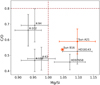 |
Fig. 5 C/O versus Mg/Si, the abundance ratios by number, for our sample of stars. The critical value of Mg/Si = 1.0 and C/O = 0.8 (Bond et al. 2010b; Suárez-Andrés et al. 2018) are indicated by the vertical and horizontal brown dashed lines, respectively. The stellar abundances (and their statistical uncertainties) are from Brewer et al. (2016), and the solar ratios (and their error bars) from Asplund et al. (2021), referred to as ‘Sun A21’, are shown for reference. The solar ratios based on abundances from Brewer et al. (2016), referred to as ‘Sun B16’, are also shown, as they are this catalog’s intrinsic solar abundances used to convert differential abundances to absolute abundances in Timmermann et al. (2023). |
3.2 Bulk elemental planetary compositions
Using the stellar composition together with the temperature-pressure profile of the disk, the condensation sequence, and our planetary accretion model, we can predict the bulk elemental compositions of the simulated planets. These estimates also depend on the timing of planetesimal formation as well as the stellar abundance pattern. As a protoplanetary disk evolves with time, the temperature and pressure in the disk decrease, and condensation fronts migrate closer to the star. As such, planetesimals forming at different times will have different compositions, even if they formed at the same distance from their star. Therefore, an important consideration is the formation time of the initial planetesimals. By a “formation time”, we refer to the timing of the thermodynamic conditions within the disk during which the planetesimals condensed out. As discussed in Sect. 2.3, formation times of 0.2 and 0.5 Myr have been suggested for the building blocks of the Solar System terrestrial planets. We do not have the necessary data to test what timing applies to our simulated systems, hence we provide results for three representative formation ages of 0.2, 0.5 and 0.8 Myr.
Figure 6 shows bulk elemental compositions (in wt%) of planets formed in five of our planet formation simulations assuming a protoplanetary disk around Kepler-62 star (the lowest metallicity star in the sample) and the formation time of planetes-imals of 0.2 Myr. Only the planets within 0.25 AU from the star are displayed as the variations between the more distant planets are very small, at the level of a few percent. The outcomes of the other simulations for this star are very similar. As we can see, the abundances approximately reflect the bulk compositions for this star in Fig. 3. The planets closest to the central star (at ~0.07 AU) contain much more Ca and Al, much less Fe and almost no Mg compared to the rest of the planets as they are mostly made of planetesimals formed at distances where Ca and Al are abundant, but Fe and Mg are almost absent. However, due to migration in the planet formation simulations, Fe and Mg are always present in those planets even if to a very small extent (particularly Mg). Not every system actually includes such a planet. For instance, simulations 1. and 4. probably lost them because they got too close to the star and were absorbed. We will discuss these so-called “Ca- and Al-rich planets”, or “Ca- and Al-rich(er)” given the high variability in their Ca and Al contents, in Sect. 4.1. The rest of the planets in each system comprise gradually less and less Ca and Al, and much more Mg, Si and Fe. Once all the solids have condensed out from the nebula, the variations in bulk elemental compositions among the planetesimals (and therefore the final planets) are not that significant and they are quite similar to the stellar abundances of the host star.
Figure 7 shows mass fractions of iron in the planetary sample depending on the distance from the host star for the highest and the lowest metallicity star, and all three formation times. As expected, planets from high metallicity stars (Kepler-94) generally have higher Fe contents than those from the lower metallicity stars, and at distances outside of 0.1 AU, the Fe content reflects the Fe abundance of their stars. However, this figure also shows that the Fe content is highly variable for the planets within ~0.1 AU from the star. For instance, The range of Fe content within ~0.1 AU ranges from nearly 0, indicating essentially coreless planets, to around 40 wt%. This wide range reflects the highly stochastic nature of planetesimal migration into the inner region of the stellar system.
In addition, the planetesimal formation time also affects the Fe mass fraction. Outside of 0.1 AU, the effect of formation time on planetary Fe composition is similar for both types of stars, with shorter formation times producing slightly more Fe-rich planets (Fig. 7), as expected from nebula temperature and condensation sequences. However, within 0.1 AU, differences between the two stars exist. For instance, in the case of the lowest metallicity star (Kepler-62), the Fe mass fractions simply increase with distance, starting lowest for the earliest formation time as the sequence begins with the highest temperatures, and then becomes constant further from the star. Overall, the highest Fe-content planets are furthest from the star. On the other hand, in the highest metallicity case (Kepler-94) the behavior is more complicated. For the earliest formation time (0.2 Myr), the Fe mass fraction first increases up to very high Fe-content planets of 40 wt%, then drops, and finally levels off, following the trend shown in Fig. 3. In contrast, for the latest formation time (0.8 Myr), there is no increase; instead, the iron mass fractions just drop with distance as the disk is cooler and the sequence begins with lower temperatures (Fig. 3). Nevertheless, regardless of formation time, the highest Fe-content planets (and largest cores) will be found nearer to the star, in stark contrast to the low-metallicity stars.
Figure 8 presents the mass of oxygen (wt%) of the planetary sample as a function of the distance from the star. The plot only shows values for one star, but the trend is representative for the whole sample. We see that again the very close planets within ~0.1 AU from the host star have a wide range of oxygen contents, showing a steep decline with the distance. The largest range again corresponds to the shortest formation time. This is also apparent in Fig. 9, which displays bulk elemental compositions generated using stellar abundances of one star and one planet formation simulation, but three different formation times. This trend is consistent across all stars and simulations, and it also shows that the innermost planets, which are richer in Ca and Al than the rest of the planets, are highly dependent on the formation time, while the other planets are affected to a much lesser extent. We also present the effect of metallic-ity for two extreme cases in Fig. 10. Here too, the difference between near and far planets is clearly visible, and metallicity only really affects the composition of near-in planets. Additionally, in case of the more distant planets (beyond ~0.1 AU), Fig. 8 initially exhibits an ascending trend as distance from the central star increases, with a sharper incline observed for later formation times. This upward trend is followed by a plateau, succeeded by another slight increase for the later formation times. The overall behavior in Fig. 8 quite accurately reflects the predicted bulk compositions, specifically the mass fraction of oxygen, as shown in Fig. 3 for this star. At first, Ti and Si appearing at around 1600 K and the Fe and Mg feature occurring at ~ 1400 K both reduce the O mass fraction, then it increases at around 1300 K and stays approximately constant until a slight increase further at much lower temperatures. This Fe and Mg feature is less prominent for lower metallicity stars. The later formation time, the cooler the disk will be and the higher oxygen content should be expected in the planetesimals, particularly in more distant regions of the disk. The scenario would differ if the location of the snow line was within of the range of planetesimals; in such a case, a rapid surge in oxygen content would be anticipated beyond the line.
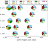 |
Fig. 6 Bulk elemental planetary compositions (in wt%) of rocky planets formed in five of our planet formation simulations assuming a proto-planetary disk around Kepler-62 star (the lowest metallicity star in the sample) and the formation time of planetesimals of 0.2 Myr. Only the planets within 0.25 AU from the star are displayed as the variations between the more distant planets are insignificant. Size of bodies is not to scale. The Earth values taken from McDonough (2014) are shown for comparison (in the upper right corner). |
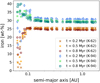 |
Fig. 7 Mass fractions of Fe in the planetary sample versus their respective semimajor axes using disk conditions around Kepler-94 (K-94; the highest metallicity star) and Kepler-62 (K-62; the lowest metallicity star) at three different formation times. |
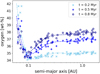 |
Fig. 8 Mass fractions of O in the planetary sample versus their respective semi-major axes using disk conditions around Kepler-62 at three different formation times. The dashed lines correspond to the polynomial fit of degree 6. |
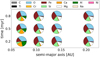 |
Fig. 9 Bulk elemental planetary compositions (in wt%) of rocky planets formed using the stellar abundances of Kepler-102. The outcome of the same planet formation simulation is shown for three different planetesimal formation times of 0.2, 0.5 and 0.8 Myr. Only the planets within 0.25 AU from the star are displayed as the variations between the more distant planets are insignificant. Size of bodies is not to scale. |
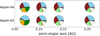 |
Fig. 10 Bulk elemental planetary compositions (in wt%) of rocky planets formed around Kepler-62 star (the lowest metallicity star), and Kepler-94 star (the highest metallicity star in the sample) assuming the same planetesimal formation time of 0.2 Myr. The outcome of the same planet formation simulation is shown in both cases. Only planets with semi-major axes within 0.25 AU are displayed. |
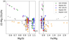 |
Fig. 11 (O–Mg–2Si)/Fe vs. Mg/Si and (O–Mg–2Si)/Fe versus Fe/Mg plots for the sample of the simulated planets around four different stars. The dashed black lines divide the planets into different types predicting different interior properties. On the left, Mg/Si = 1.0 is the division between more pyroxene-rich (Mg/Si < 1.0) and olivine–pyroxene mixed (Mg/Si > 1.0) mantles. On the right, the Fe/Mg = 0.9 line separates the planets with potentially smaller cores (Fe/Mg < 0.9) and potentially bigger cores (Fe/Mg > 0.9). Above the horizontal line at (O–Mg–2Si)/Fe = 1, the planets are expected to be more oxidized, and below typically less oxidized. The values for the Earth (Wang et al. 2018) and Mars (Yoshizaki & McDonough 2020) are shown for reference. The planetesimal formation time of 0.8 Myr is assumed here. |
3.3 Key planetary geochemical ratios
The most important elemental ratios to determine the first order mineralogy and interior structure (i.e., core mass fraction) of a rocky planet are C/O, Mg/Si and Fe/Mg. By calculating the C/O and Mg/Si ratios for our star sample, we have already shown that the simulated planets should be dominated by silicates (not carbides), produced with either SiO44− or SiO2 as building blocks, since the C/O ratios are under 0.8 for all the stars (see Sect. 3.1).
Figure 11 presents (O–Mg–2Si)/Fe versus Mg/Si and (O–Mg–2Si)/Fe versus Fe/Mg plots for the sample of the simulated planets around five of our stars. We omitted Kepler-113 here because it overlaps with other values and does not provide new information. Planetary Mg/Si values match their respective stellar Mg/Si ratios for majority of the planets, and imply a potentially Earth-like olivine-pyroxene mixed mantle compositions for most of the planets formed around HD 97658 and HD 18143. However, in some cases these ratios are significantly different, indicating the existence of Mg-depleted (compared to Earth) planets as predicted already in Carter-Bond et al. (2012a). For the Mg-depleted planets orbiting HD 97658 and HD 18143, the disparity should even lead to differences in the dominant mineral compositions in their mantles, potentially favoring pyroxene over olivine-pyroxene assemblages, which are expected for the rest of the planets around these two stars. The Fe/Mg ratio, on the other hand, is often used as an indicator of the degree of core-mantle fractionation, so it can provide us with a very rough estimate of the size of a planetary iron core. Additionally, the bulk (O–Mg–2Si)/Fe of rocky exoplanets was proposed as an indicator of a mantle oxidation state (i.e., an alternative to oxygen fugacity, fO2; Wang et al. 2022b), as the data required to calculate fO2 for exoplanets are not available. Knowing the oxidation state of a planet can also help us to estimate the core size of the planet, with more oxidized mantles typically resulting in smaller iron cores (oxidized Fe is locked in the mantle) and vice versa, as well as initial atmospheric formation conditions.
Considering solely (O–Mg–2Si)/Fe, we would expect almost all the displayed planets to be more oxidized than the Earth, and therefore have core mass fractions smaller than the Earth, and in many cases comparable to Mars or even smaller. Whereas based on the Fe/Mg ratio, the planets orbiting the Kepler-102 and Kepler-94 stars are anticipated to develop bigger cores than the Earth, although not by much. Both of these stars have higher metallicity than the Sun, however Kepler-102 only slightly. Several planets exhibit very high Fe/Mg values, but those are the already mentioned Mg-depleted planets, so their high Fe/Mg ratios are actually due to very low Mg content and not due to high Fe content. Nevertheless, the apparent inconsistency in the implications of (O–Mg–2Si)/Fe versus Fe/Mg can be explained by the fact that these two ratios have slightly different meanings. Fe/Mg is less powerful than (O–Mg–2Si)/Fe in indicating core mass fraction, as the former only works well if the oxygen fugacity of a planet is not significantly different from Earth’s. Otherwise, the Fe/Mg ratio is less sensitive in indicating core mass fraction due to the discrepancy in partitioning Fe between FeO and metallic iron. However, this can be well represented in the (O–Mg–2Si)/Fe ratio, as it contains information on both the silicate portion and oxygen fugacity (its proxy). This also applies to Mg-depleted cases, as long as the planets are silicate, but it may not work for the Ca- and Al-rich planetary bodies, which partially overlap with Mg-depleted planets. For Fig. 11, we assumed the planetesimal formation time of 0.8 Myr. Generally, with later formation the (O–Mg–2Si)/Fe values of the formed planets are higher, since more O is available (shown already in Sect. 3.2).
Figure 12 shows Mg/Si versus Al/Si for the same sample of stars/planets as in Fig. 11. The plot illustrates a steady transition in composition, but with a clear division between the ratios comparable to the Earth/Mars ratios (in the upper left quarter), and the higher Al/lower Mg ratios (in the lower right quarter). In the plot, a significant proportion exceeding 80% of the data points with Al/Si closest to 0 for each star actually overlap. The planetesimal formation time of 0.8 Myr is assumed here, but the diagram is representative for all three formation times. However, when sooner formation times are selected, the dataset extends to the right towards even higher Al and lower Mg values, particularly in case of these Al-enriched planets, reaching the maximum of Al/Si ~4 and minimum Mg/Si close to 0. This plot illustrates that these Mg-depleted planets (already shown in Fig. 11) are the same objects as the innermost Ca- and Al-rich(er) planets displayed here and already in Fig. 6. Further in the paper, the analyses made in this section will be confirmed through more detailed modeling of the interiors.
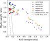 |
Fig. 12 Mg/Si versus Al/Si weight ratios for the sample of the simulated planets around four different stars. In the plot, more than 80% of the data points with Al/Si closest to 0 for each star actually overlap, so only the planets with higher Al/Si are fully and individually displayed. The values for the Earth (McDonough 2014) and Mars (Yoshizaki & McDonough 2020) are shown for reference, together with their frac-tionation lines (the gray dashed lines). The planetesimal formation time of 0.8 Myr is assumed here. |
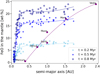 |
Fig. 13 Mass fractions of FeO in the mantle in the planetary sample versus their respective semimajor axes using disk conditions around Kepler-102 – whose metallicity is closest to the Sun’s – at three different formation times, with varying shades of blue indicating the progression of time. The blue dashed lines correspond to the polynomial fit of degree 3. In contrast, the purple squares denote the FeO mass fractions of terrestrial Solar System bodies (Trønnes et al. (2019), Table 2) as a function of their distances from the Sun. The purple dashed line represents the best fit for better visualization. |
3.4 Mass fraction of FeO in the mantle
Based on the oxidation sequence described in Sect. 2.4, we estimated the mass fraction of FeO in the mantles of the simulated planets. Figure 13 shows these mass fractions versus their respective semimajor axes using disk conditions around Kepler-102 at three different formation times, together with the mass fractions of the terrestrial Solar System bodies. As expected, the figure demonstrates a pattern similar to Fig. 8, since the values depend primarily on the available amount of oxygen in a planet. The other stars display similar trends, but with generally lower FeO fractions for lower metallicity stars and higher FeO fractions for higher metallicity stars. We chose Kepler-102 stellar abundances for this plot to be able to compare the fractions to the mass fractions of mantle FeO in the terrestrial Solar System bodies. In the case of asteroid Vesta, which is a much less massive body than all the rest (with approximately 0.4% of a lunar mass), the value should be interpreted with caution as partitioning of oxygen between the mantle and core in such a small object can happen a bit differently. Kepler-102 is the closest star to our Sun in terms of metallicity, and we can see that the FeO mass fractions in Fig. 13 for this star are comparable to the values in our Solar System, if we consider all three formation times. This aligns with the assumption that building blocks of planets likely formed from material from a range of formation locations and times. In general, planetary bodies that formed at lower temperatures (i.e., later or further from the star) exhibit higher percentages of oxidized iron in their mantles. This figure suggests that the simulated systems are oxidized similarly to the rock-forming materials in the Solar System. However, their distances from the Sun/star may not be directly comparable, as the bodies orbit stars of different masses and spectral types.
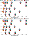 |
Fig. 14 Interior composition (in wt%) of the simulated planets in five different systems around Kepler-62 (the lowest metallicity star). The planetesimal formation times of 0.2 Myr (the top five simulations) and 0.8 Myr (the bottom five simulations) are assumed. Only planets with semimajor axes within 0.4 AU are displayed. The Earth values taken from McDonough (2014) are shown for comparison (the upper right corner). |
3.5 Interior composition and structure
Interior composition of the final bulk planets was computed using the oxidation sequence: Na2O–CaO–MgO–Al2O3– SiO2–FeO–NiO–SO3–CO2–C(graphite/diamond)-metals, and it is presented in Figs. 14 and 15. All Fe, Ni and S that are not oxidized (i.e., they are reduced) are included in the core. Figure 14 shows the simulated planets in five different systems around Kepler-62 (the lowest metallicity star) assuming the planetesimal formation times of 0.2 Myr (the top five simulations) and 0.8 Myr (the bottom five simulations). Obvious radial compositional variations can be seen in all simulated systems, which show very similar pattern when applying the same stellar abundances. Later formation time typically results in more oxidized planets, particularly in case of the more distant planets (as shown already in Sect. 3.4), and in compositions of the odd innermost planets that are less extreme compared to Earth’s. If formed quickly (i.e., 0.2 Myr), these Ca- and Al-rich(er) planets exhibit very small, or basically no core at all. Their interiors are dominated by CaO and Al2O3 and completely depleted in MgO. The bulk composition of the more distant planets is not that different from the composition of the Earth, except for the mass fractions of the core and SiO2, at least in case of the shorter formation time. This is due to the fact that Kepler-62 has lower metallicity and more Si (compared to the other main rock-forming elements) in comparison to the Sun. Only planets with semimajor axes within 0.4 AU are displayed in the plots as the more distant planets follow the same trend with minimal further variations. This outcome is anticipated. Generally, volatile budgets can vary significantly among planets formed in the same disk (e.g., Öberg & Bergin 2016), but the planets have usually quite similar budgets of relatively refractory elements (e.g., Sotin et al. 2007; Bond et al. 2010a; Thiabaud et al. 2014). Figure 15 displays four different systems assuming the stellar abundances of Kepler-94 (the highest metallicity star). The pie charts illustrate generally larger cores, especially in case of the shorter formation time. The Ca- and Al-rich(er) planet is not core-less in this instance, but it is MgO depleted and its core is smaller than in the rest of the system’s planets. We also predict a high degree of oxidization for the more distant planets formed on 0.8 Myr timescales. Figures 14 and 15 would display similar oxide fractions for the other stars as well, with the largest differences occurring in their core fractions, depending on the stellar metallicities.
Figure 16 depicts three core mass fraction plots, computed using ExoPlex (Unterborn et al. 2023), for the whole simulated planetary sample around Kepler-94 and Kepler-62 (highest and lowest metallicity star) as a function of their distance from the star. The lower and upper limits correspond to the planetesimal formation time of 0.8 and 0.2 Myr, respectively, with a few exceptions in the case of the Ca- and Al-rich(er) planets when the two values are switched. The behavior illustrated in the plots is similar to the trends in Fig. 7, which shows only the Fe abundance with the distance from the star. Again, we see that core mass fractions typically increase with distance for the lowest metallicity star (Kepler-62), and mostly decrease with distance for the highest metallicity star (Kepler-94). Also, it is obvious and expected that higher metallicity produces larger cores. The same is generally true for shorter formation times as well. Here, we present two extreme cases of largest and smallest core mass fractions around Kepler-94 and Kepler-62, respectively, while the systems around the rest of the stars lie somewhere between the two extremes. Plot A presents core mass fractions (wt%) of the planets, where the cores contain only pure Fe. It is evident that with only Fe, we are able to produce planets with core mass fractions of the Earth or higher only close to the star and assuming a high metallicity star. We can form planets with core mass fractions of Mars at all distances, but mostly only in case of the metal-rich star. It seems that the simulated planets are generally more oxidized than the Earth, and consequently have smaller cores. Decreasing the amount of oxygen in their bulk compositions by approximately 5% would enlarge their cores to around Earth’s iron core mass fraction, for the metal-rich star Kepler-94. In Plot B, we plotted core mass fractions (wt%) of the cores containing Fe and reduced Ni and S in the oxidation sequence, similarly as in Figs. 14 and 15. All core mass fractions naturally increase compared to the pure iron scenario, but the core mass fractions of the planets located further out (> ~0.1 AU) increase much more than in case of the closer planets. This is due to the temperatures being cool enough for solid S to occur further out from the host star. As recommended in Wang et al. (2019b), the upper limit of the Ni and S content in the core are their abundances in the bulk planet; as for the Earth more than 90% of Ni and 95% of S are in the Earth’s core (McDonough 2014; Wang et al. 2018). The lower limit is nil, such as in a rare scenario when all metals including Fe are fully oxidized resulting in core-less planets (Elkins-Tanton & Seager 2008). Figure 16 shows several such planets in all three plots around Kepler-62 very close to the star. The upper limit of the Ni and S content can in some cases be quite high, when compared to the values from the Solar System. For example, 14 wt% of the Earth’s core (McDonough 2014), 20 wt% of the Mars’ core (Yoshizaki & McDonough 2020) and 14 wt% of the Mercury’s core (McDonough & Yoshizaki 2021) are believed to be composed of elements other than Fe (Ni and the lighter elements), whereas in some of the simulated planets the number is up to 30–35 wt%, resulting in the increase of core mass fractions of up to around 6–7% if all Ni and S in a bulk planet (not oxidized in the oxidation sequence) are incorporated into the core. It seems that in contrast to the equilibrium chemistry, where S species are not expected to play a major role for our stars (see Sect. 2.2), S is quite important in planetary geochemistry for the interior composition. In Plot C, we see core mass fractions (wt%) of the cores containing Fe and reduced Ni and S, and in addition reduced Si. In this scenario, we allowed for the potential partial oxidation of Si (as mentioned in Sect. 2.4), and reduced Si ended in the core. The core mass fractions are now a bit higher, typically between 1 and 2%, than in the plot B as the cores contain even more of lighter elements. Now, the planets have mostly up to 5–6 wt% of Si in their cores, however, in some of these exotic innermost planets the percentage can be much higher. In comparison, Earth contains approximately 4 wt% (McDonough 2014) and Mercury 4.1 wt% (McDonough & Yoshizaki 2021) of Si in their cores.
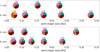 |
Fig. 15 Interior composition (in wt%) of simulated planets in four different systems around Kepler-94 (the highest metallicity star). The formation times of 0.2 (6. and 7. sim) and 0.8 Myr (8. and 9. sim) are assumed. Only planets with semimajor axes within 0.4 AU are displayed. The legends from Fig. 14 also apply to this figure. |
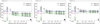 |
Fig. 16 Core mass fractions, computed using ExoPlex (Unterborn et al. 2023), for the simulated planets around Kepler-94 and Kepler-62 as a function of their distance from the star. The lower and upper limits are calculated for the planetesimal formation time of 0.8 and 0.2 Myr, respectively. Plot A: Core mass fractions (wt%) of the planets, if the cores contain only pure Fe. Plot B: Core mass fractions (wt%) of the cores containing Fe, and reduced Ni and S. Plot C: Core mass fractions (wt%) of the cores containing Fe, and reduced Ni and S, and in addition reduced Si. The core mass fractions for our terrestrial planets, Mercury = 68 wt% (Smith et al. 2012), Earth = 32.5 wt% (Wang et al. 2018), and Mars = 25 wt% (Khan et al. 2022), are shown for comparison. |
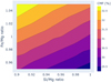 |
Fig. 17 Core mass fraction versus Fe/Mg and Si/Mg molar ratios, where the ranges reflect the uncertainties in the stellar abundances. The core mass fractions, computed using ExoPlex (Unterborn et al. 2023), are of a typical simulated planet of 1 M⊕ around Kepler-94 assuming the planetesimal formation time of 0.2 Myr. |
3.6 Sensitivity to uncertainties in stellar abundance measurements
Additionally, to illustrate how core mass fraction values are influenced by the uncertainties in stellar elemental abundances, Fig. 17 displays a plot with core mass fractions of a typical simulated planet of 1 M⊕ (however, a different mass would not change the core mass fraction values) around Kepler-94 assuming a planetesimal formation time of 0.2 Myr. The core mass fraction versus Fe/Mg and Si/Mg molar ratios show the variations in the core mass fraction up to 3%. The ranges of ratios are determined by the uncertainties in stellar abundances that are all around 0.01 dex in case of Fe, Si and Mg (Brewer et al. (2016), Table 6). The uncertainties are then propagated to the core mass fraction uncertainties of ±3%. Naturally, this applies specifically to the catalog used in this study and would vary for other catalogs of stellar abundances.
Altogether, Figs. 14, 15, and 16 cover all possible types of planets that emerged from our simulations, namely: Ca- and Al-rich(er) planets, Mg-depleted, fully oxidized core-less planets, planets similar to Earth or Mars in composition and core size, and planets with different core mass fractions (from significantly smaller than the Martian core to significantly larger than the Earth’s core), but no Mercury-like planets with a huge iron core. In addition, we managed to form planets with extremely small cores, such as our Moon, with a core mass fraction <2 wt% (Viswanathan et al. 2019); however, those are the Ca- and Al-rich(er) planets with very different compositions compared to the Earth or Moon. For a silicate planet, such as our own, MgO and SiO2 are the foremost mineral oxides in the mantle, but this is not always the case for these odd innermost planets. Throughout the study, the code was executed consistently with a constant mantle potential temperature of 1600 K, as the test runs with temperatures of 1500 and 1900 K, a typical range used in similar studies (e.g., Hinkel & Unterborn 2018), yielded no significant variations.
Even though, our model does not generate previously proposed higher-mass analogs of Mercury, so-called “superMercuries” (e.g., Marcus et al. 2010; Adibekyan et al. 2021), it does form planets with larger cores (up to ∼50 wt%) compared to the rest of the system, which are always the innermost planets. We managed to form them around the stars with the metallicity similar to the Sun’s metallicity and higher. This suggests that a giant impact is still necessary to explain the high density of a super-Mercury.
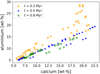 |
Fig. 18 Mass fractions of Al versus Ca in the planetary sample using disk conditions around all six stars at three different formation times. Only bodies with both values above 5 wt% are displayed. For comparison, bulk Earth contains 1.59 and 1.71 wt% (McDonough 2014), and bulk Mars 1.56 and 1.69 wt% of Al and Ca, respectively (Yoshizaki & McDonough 2020). |
4 Discussion
4.1 Ca- and Al-rich(er) planetary bodies
In this section, we discuss the Ca- and Al-rich(er) bodies introduced in Sect. 3.2. These are the innermost objects occurring in around 40% of our planet formation simulations, with masses roughly between 1.5 and 2.5 M⊕. They are found within approximately 0.07 AU from their host star, however, as the planetary Ca and Al mass fractions decrease gradually as a function of distance from the star, some simulated bodies with higher Ca and Al fractions than the rest of the planets in a system can be found to about ∼0.1 AU (see Fig. 6). The interiors of these objects are built from high-temperature condensates (>1200 K), therefore they are rich in Ca, Al and O, and often low at Mg, Si and/or Fe, depending on the simulation, selected formation time and elemental abundances of the host star.
Figure 18 shows the mass fractions of Al versus Ca in the planetary sample around all six stars at three different formation times. Earlier formation time (and therefore hotter disk) results in more planetary bodies enriched in Ca and Al being produced in the sample, and they typically contain higher Ca and Al abundances than those formed later. Maximum mass fractions for Ca are between 19 and 23 wt% and for Al from 15 to 29 wt%, depending on the formation time. The existence of such objects was already predicted in Carter-Bond et al. (2012a), also with N-body simulations, and in Thiabaud et al. (2014). Both studies, like ours, assumed chemical equilibrium in the disk. However, Thiabaud et al. (2014) estimated much greater elemental compositions for Al (40–50 wt%) than for Ca (7–9 wt%). Our work suggests that these objects should actually have similar weight fractions for these two elements due to migration and radial mixing of planetary building blocks, something not taken into account by the other study. In addition, Thiabaud et al. (2014) found Ca- and Al-rich planets within 0.3 AU, while we found them closer to their host stars (<0.1 AU). This is not unexpected since their planets formed in solar nebula, whereas we focused on less massive stars and more compact systems. Thiabaud et al. (2014) found Ca- and Al-rich objects with masses ofup to 3 M⊕, which agrees with our findings. Simulations of Carter-Bond et al. (2012a) generated bodies with similar percentages of Ca and Al to ours, but within 0.5 AU, as they also studied more massive stars than this work.
The unusual bulk composition of these objects should result in their bulk density being lower in comparison to other planets within their respective systems. Dorn et al. (2019) explored a possibility of this new class of super-Earths to explain several examples of observed exoplanets with lower bulk densities than expected, and demonstrated that planetary bodies made of high-temperature condensates and depleted in Fe (possibly even core-less) would be about 10–20% less dense than Earth-like compositions. Of course, volatile-rich interiors could also be the reason of lower density of the objects, however very close proximity to their host stars makes it less likely. We will look more into this in Sect. 4.2. Before proceeding to the next section, it is important to address one more issue.
A protoplanetary disk is affected by stellar activity, such as stellar winds and photoevaporation. Stellar winds can gradually strip away gas and dust from the disk, while photoevaporation, caused by high-energy radiation from the star, can heat and disperse the gas disk. This can influence masses and compositions of the planets, particularly those forming closest to the star. In our simulations, the innermost Ca- and Al-rich(er) objects have masses of a several M⊕, but due to these processes, there might not be that much mass available so close to the star as the high- temperature condensates might be partially re-distributed into the disk. Particles similar to Calcium-Aluminum-rich Inclusions (CAIs) have been found in materials originating from various parts of the Solar System, including the outer regions (e.g., Davis 2005; Sunshine et al. 2008). However, the processes would mainly reduce the in-situ amount of mass in the stellar proximity, whereas our innermost planets have these ‘high’ masses as a consequence of orbital migration, mergers and giant impacts. They are the natural outcomes of our planet formation simulations, where compositions were included during post-processing. In summary, the existence of Ca- and Al-rich(er) bodies with planetary masses may be uncertain, but for the purpose of this study, we refer to them as planets. It would be interesting to address this issue in a future study.
4.2 Comparison to the known systems
Based on the composition of the bulk planets presented in Sect. 3.5, we calculated the planetary radii using ExoPlex and compared the simulated systems to the observed systems. Although we have an observed sample of 139 planets orbiting K dwarfs described in detail (in Sect. 2.1), for this analysis we only consider presumably rocky planets with masses of ∼7 M⊕ or less, as we did for the simulated population, therefore the final observed sample contains only 40 known planets. Figure 19 displays the mass-radius relationship showing the simulated planetary sample, assuming a formation time of 0.2 Myr (later formation times do not change the plot significantly), together with the observed population. Both the simulated planets with compositions similar to Earth and some of the simulated Ca- and Al-rich(er) planets are displayed. For many of these innermost Ca- and Al-rich(er) planets, we were not able to compute radii and densities, as their compositions are way too different from the Earth’s composition and the code is not designed to accommodate this. Hence, the densities and radii of the Ca- and Al-rich(er) bodies could be examined in future research. As can be clearly seen, the observed population exhibits a much greater range of mass to radius than our simulated planets, which presumably reflects a much larger variation in chemical compositions, particularly, in their volatile content. However, the limited compositional range of our planets was anticipated as we are currently focused only on rocky silicate planets without tracking the volatiles. Nevertheless, we found that according to the mass-radius relationship the majority of the simulated planets are not very unlike the terrestrial Solar System planets, with the variations being mostly within the 20 to the 30%Fe curves, or slightly over. Typically, the planets are compositionally like more or less massive versions of Earth and Venus. This aligns with the elemental abundances observed in polluted white dwarfs, suggesting that most exoplanetary systems likely produce rocky bodies with compositions similar to chondritic meteorites in our Solar System (Hinkel & Young 2024). The more exotic innermost planets almost reach the rock and the 50%Fe curves, corresponding to the (almost) core-less planets and the planets with relatively large cores, respectively.
Table 5 contains the data for several examples of the Ca- and Al-rich(er) planets (some of the light-green circles in Fig. 19), assuming the formation time of 0.2 Myr. The properties are computed for pure Fe cores and ordered by the increasing distance from the host star. The asterisk(*) is used to denote the radii of planets as homogeneous spheres calculated based on the mass from the dynamical simulations and the density of 3 g cm–3 for each planet. This value is commonly assumed for rocky planetesimals formed in the inner part of a protoplanetary disk. Due to the gravitational effects compressing the mantle, the radii computed using ExoPlex are always smaller and densities higher than 3 g cm–3. For comparison, Earth has the highest bulk density of any planet in the Solar System at 5.51 g cm–3, and iron density is 7.87 g cm–3. The more massive planet the more compression is expected. The first two planets, even though being somewhat more massive than the Earth, have densities lower than our planet due to their very small cores. On the other hand, the last two planets with masses of ∼6 and 7 M⊕ have very high bulk densities, even higher than iron, without having super large iron cores. This might seem a bit odd; however, these planets are much more massive than Earth, so their high densities can be attributed to a combination of composition (heavy metals, compressed phases) and extreme gravitational compression. Also, incorporating volatiles into the compositions of our simulated planets would at least slightly decrease their densities. Table 5 presents the characteristics of the same planet 1. Sim b (the innermost planet in one of the planet formation simulations) assuming the abundances of three different stars. This illustrates potential variations in the planets formed around the stars with different metallicities; for instance, comprising up to 20 wt% in their core mass fractions. Yet, these variations have minimal impact on the radii of the planets (about 2–3%) and are basically undetectable at the moment, as the current distribution of radius uncertainties for exoplanets peaks at around 8% (Otegi et al. 2020).
The final comparison of the simulated versus observed planet population around K dwarfs is shown in Fig. 20. Here, our focus is again only on the known planets with a super-Earth mass of ∼7 M⊕ or less (so without substantial amounts of accreted gas), although the simulations also produced several planets with higher masses. We display both the simulated population with the radii of planets as homogeneous spheres with one preset average density (3 g cm–3) for all bodies, and the simulated population with compressed radii and individual ρ. The latter population exhibits smaller radii, as expected. There is a significant region where the observed and simulated samples overlap, which shows that we managed to reproduce the observed population at least partially. However, ExoPlex can model planetary characteristics only up to ∼2 R⊕, therefore we do not see any planets with compressed radii in the upper region of the plot. Additionally, as explained in detail in Hatalova et al. (2023), our planet formation simulations were limited by an inner truncation radius of 0.05 AU due to computational constraints, even though many known systems around K dwarfs contain planets with shorter orbital distances. Therefore, for some analyses of the previous study we moved all the simulated planets closer to the star by this distance, as was also done in Fig. 20. Our simulated systems also contain many small planets mostly at larger distances, which are basically undetectable by the current methods. These are located in the bottom right corner of the plot, where no observed planets have been found so far. Therefore, studies like this are important for the design of surveys searching for terrestrial planets in exoplanetary systems.
 |
Fig. 19 Mass-radius diagram (on the left) showing the simulated planetary sample (black circles, often partially overlapping), assuming the formation time of 0.2 Myr, together with the observed K-dwarf population (blue circles with gray error bars), and the terrestrial Solar System planets for comparison (red circles). Some of the simulated Ca- and Al-rich(er) planets are also displayed (light-green circles). The compositional curves are from Zeng et al. (2016). The plot on the right is just a zoomed-in version of the gray dashed region in the left diagram. |
Data of some of the Ca- and Al-rich(er) planets computed using the ExoPlex code assuming the formation time of 0.2 Myr.
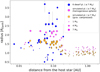 |
Fig. 20 Radii versus semimajor axes of our simulated planetary systems, both the radii of planets as homogeneous spheres calculated based on ρ = 3 g cm–3 (in magenta), and the compressed radii with individual ρ (in orange), compared to the currently known systems around K dwarfs (in blue). Only planets with known masses of 7 M⊕ or less are presented. The point size indicates the masses in M⊕ of the planets. |
4.3 Study limitations
One of the limitations inherent in this study is the fact that in condensation equilibrium simulations the pressure is kept constant during the entire simulation. The pressure was chosen in accordance with the disk profile and planetesimal formation time, as described in Sect. 2.3. Specifically, we selected the maximum pressure value in the disk profile (the value closest to the star) as the constant for the whole disk. However in a real disk, the disk pressure would be reduced with the decreasing temperature and gas surface density as a function of time and distance from the central star. Nevertheless, as disk pressure affects the condensation temperatures of all studied elements in a similar way (Timmermann et al. 2023), it is anticipated that variations in pressure would simply move the equilibrium composition to higher temperatures with increased pressure and vice versa. They should not lead to any qualitative changes in the estimated composition.
Another important limitation is that a planet probably accumulated material from a range of locations and times during its formation due to orbital migration, an aspect that is only partially integrated into this study. The possible formation location range is between 0.2 and 2 AU from the star, which means that planets that formed close to the outer edge would probably have grown larger if there was an influx of material from larger distances (> 2 AU) inwards. It is evident that more distant planets are less massive than those closer to the star (see again Fig. 1). For the same reason, their compositions could have been a bit different as well. Even more importantly, we assume that all building blocks in a system formed at the same time, which is clearly not realistic. The formation timing affects the temperature profile of the disk, as shown in Appendix B, and therefore also bulk composition of planetary building blocks and the resulting planets.
One more issue related to the planetesimal formation time is that we modeled planetesimal compositions based on the chemical equilibrium in the disk at three distinct times, meaning all planetesimals formed instantaneously at one of these times. These condensation simulations were not done sequentially over time, which would be more realistic, namely, the condensation at later time is not impacted by the condensation that occurred earlier. However, planetesimals form over an extended time period during which elements sequentially condense out from the gas as the disk cools and are subsequently accreted onto the planetesimals. We did not account for the evolution of the disk during planetesimal formation in this study. This simplified one-time condensation should limit the diversity of the condensates (and thus planetary building blocks) over time. However, including the sequential condensation would make our post-processing much more complicated, as the software we used is not designed to accommodate it.
An additional consideration is the disk temperature profile. We employed the profile of Chambers (2009), which has been previously used in similar studies (e.g., Moriarty et al. 2014; Alessi et al. 2017; Harrison et al. 2018; Dorn et al. 2019).
However, researchers studying protoplanetary disks and planet formation typically prefer generally colder temperature profiles (e.g., Ida et al. 2016), where the temperature at 1 AU can be up to several hundred Kelvin lower depending on the time in the disk’s evolution. However, this cool temperature is difficult to reconcile with the estimated Earth’s formation temperature, which is between 1100 K and 1400 K, based on the depletion pattern of volatile elements in the Earth (Wang et al. 2019a; Sossi et al. 2022). This issue deserves further attention.
In future research, it would be beneficial to address these limitations, together with the issue regarding the likelihood of the existence of Ca- and Al-rich planets discussed in Sect. 4.1, and incorporate additional factors to the simulations, such as the contribution of volatiles to estimates of planetary compositions, or the formation and migration of giant planets, which are expected to alter the composition of final rocky planets.
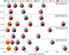 |
Fig. 21 Interior compositions (in wt%) of the simulated planets in eight different systems around Kepler-62 (the lowest metallicity star) and Kepler-94 (the highest metallicity star) assuming the planetesimal formation times of 0.2 Myr (the earliest formation time) and 0.8 Myr (the latest formation time). The systems are grouped in pairs and selected to showcase all possible categories of planets that emerged from our simulations. Only planets with semimajor axes within 0.4 AU are displayed. The Earth values taken from McDonough (2014) are shown for comparison (lower right corner). |
5 Conclusions
We incorporated stellar abundances from six K-dwarf stars with different metallicities into our N-body simulations around a 0.8 M⊙ star based on a chemical equilibrium in a protoplanetary disk. We then developed models of likely compositions and radii of rocky exoplanets using the condensate composition as a proxy for planet composition. Our conclusions are given below:
Condensation sequence based on chemical abundance pattern of a star and equilibrium chemistry in a protoplanetary disk is reflected in the planetary geochemical ratios of the simulated systems and, hence, in their compositions and interior structures;
The simulated planets located within the innermost region around a star (< ~0.1 AU) have Al/Si and Ca/Si ratios well above the Solar System terrestrial planet values, whereas Mg/Si is typically well under. The planets located further out (> ~0.1 AU) have strongly homogeneous bulk planetary compositions, which still reflect their host star chemical abundances. In this region, the planetary Mg/Si, Al/Si, and Ca/Si values are comparable to Earth values. There is a smooth transition in composition between these two regions;
Figure 21 displays all possible planet categories that emerged from our simulations assuming different formation times and stellar metallicities. The dynamical input parameters (initial disk mass and surface density values) do not have significant impact on the planetary compositions for the purpose of this study; therefore they are not taken into account in the plot. These categories are: Ca- and Al-rich(er) planets, Mg-depleted planets (compared to Earth; consisting of silicate species such as pyroxene and various feldspars), fully oxidized core-less planets, planets similar to Earth or Mars in composition and core size, and planets with different core mass fractions (from significantly smaller than the Martian core to significantly larger than the Earth’s core), but no Mercury-like planets with a huge iron core. In addition, we managed to form planets with extremely small cores, but those are the Ca- and Al-rich planets with very different compositions, as compared to the Earth or Moon;
The majority of simulated exoplanets seem geophysically and geochemically similar to Earth or Mars. The largest variations in the compositions of the planets come from radial compositional variations in the protoplanetary disk, as well as in the inner regions of the systems, and from the differences in the chemical abundances of the host stars, in the outer regions of the systems;
The simulated planets have generally smaller core mass fractions compared to the Earth, but whether the oxidation of rocks in the Earth can be assumed for rocky planets in other planetary systems is unknown. Losing some amount of oxygen during the accretion process could increase our estimates. In this study, we do not consider volatile loss during accretion, which is assumed to be quite significant for Solar System evolution. Alternatively, the devolatilization pattern has been quantified for the Earth, but it is uncertain to what degree it can be extended to exoplanets. Since this process depletes oxygen more than any other major rockforming element included in this work, it could also affect our estimates.
Acknowledgements
We thank the editors and the anonymous reviewer for their constructive comments, which have helped improve this paper. This study is supported by the Research Council of Norway through its Centres of Excellence funding scheme, project No. 332523 PHAB. It has been done at the Centre for Planetary Habitability (PHAB) at the University of Oslo. Our numerical simulations have been performed on the Norwegian supercomputer Betzy operated by Sigma2 as a part of Stephanie C. Werner’s project NN9010K. The authors would like to thank Simon Grimm and Joachim Stadel for allowing them to utilize their software GENGA, Anina Timmermann for her software ECCOplanets, and Cayman Unterborn for providing significant assistance with the use of his software ExoPlex. The study has made use of the NASA Exoplanet Archive operated by the California Institute of Technology, and The Extrasolar Planets Encyclopaedia (exoplanet.eu). Additionally, the authors acknowledge the help from the members of the Earth and Beyond group at PHAB.
Appendix A [S/H]-[Fe/H] correlation
Sulfur is easier to measure in FG-dwarfs than in cooler stars. To estimate the sulfur abundances of our K-dwarf stellar hosts (Sect. 2.2), we examined the correlation between [S/H] and [Fe/H] for a sample of FG-dwarf stars in the solar neighborhood. We obtained [S/H] and [Fe/H] abundances for all stars with Teff between 5500 and 6500 K and log(𝑔) > 4.0 from the Hypatia Catalog2 (Hinkel et al. 2014), shown in Fig. A.1. Since they exhibit a strong linear correlation. we fitted a simple linear model uses a robust least absolute deviation method with the IDL ladfit routine. The best-fit relation is given by:
![$[{\rm{S}}/{\rm{H}}] = - 0.018 + 0.73[{\rm{Fe}}/{\rm{H}}]$](/articles/aa/full_html/2025/02/aa51070-24/aa51070-24-eq2.png) (A.1)
(A.1)
as shown in Fig.A.1. This relation has a mean absolute deviation of 0.092 dex. Assuming chemical abundance patterns for K-dwarfs are similar to that for FG-dwarfs, Eqn. A.1 can be used to approximate S abundances for cool dwarfs whose Fe abundances are known.
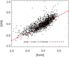 |
Fig. A.1 Sulfur vs. iron abundances for a sample of nearby FG dwarfs. Data taken from the Hypatia Catalog (Hinkel et al. 2014). The red dashed line shows the best-fit and is used to approximate sulfur abundances for our K-dwarf stellar hosts. |
Appendix B Protoplanetary disk model
The temperature profile of the protoplanetary disk together with the pressure and surface density are calculated using an established theoretical model with an alpha parameterization derived in Chambers (2009), which describes an evolving viscously heated and irradiated disk. The model divides the disk into three regions: an inner viscous evaporating section, an intermediate viscous section, and an outer irradiated section. In the inner and intermediate regions the disk is heated primarily by viscous dissipation, whereas in the outer region it is the stellar irradiation that dominates the heating of the disk, as viscous dissipation does not generate significant amounts of energy in this section. Here, t is the time since the formation of the disk, r is the distance from the star (radius), M0, s0 and Ω0 are the initial mass, radial extend of the disk, and the orbital angular velocity, respectively. M*, R*, and T* are the mass, radius and temperature of the star. The viscosity parameter α = 0.001, which is a commonly assumed value used in similar studies.
In the inner viscous evaporating region of the disk, the temperature is given by
 (B.1)
(B.1)
where Tvis is the viscous heating temperature constant defined as
 (B.2)
(B.2)
and Te = 1380 K according to Stepinski (1998), which is the temperature at which most solids evaporate. The viscous timescale τvis equals
 (B.3)
(B.3)
where Σvis is a constant
 (B.4)
(B.4)

In these formulas, kB is the Boltzmann’s constant, σ is the Stefan-Boltzmann constant, γ = 1.4 is the adiabatic index, mH is the mass of a hydrogen atom, and µ = 2.4 is the mean molecular weight. In this innermost region where T > Te, the opacity κ follows the power law from Stepinski (1998) and is expected to be much lower than in the rest of the disk as most solids cannot condense out at these temperature, therefore
 (B.6)
(B.6)
while at lower temperatures κ is assumed to be basically constant κ0 = 3 cm2/𝑔. The transition radius between the inner and the intermediate viscous regions is
 (B.7)
(B.7)
where Σevap is another constant
 (B.8)
(B.8)
The surface density in the region follows
 (B.9)
(B.9)
In the intermediate viscous region of the disk, the temperature is given by
 (B.10)
and the surface density equation is
 (B.11)
The temperature in the outer irradiated region is
 (B.12)

The transition radius between the intermediate viscous region and the outer irradiated region is given by
 (B.14)

The surface density equation is
 (B.16)
At last, using the ideal gas equation of state we can obtain the mid-plane pressure from the surface density and mid-plane temperature as follows:
 (B.17)
where ρM is the mid-plane density
 (B.18)
and H represents the scale-height of the disk
 (B.19)
Here, we assume that the disk consists of an ideal gas with a Gaussian density profile
 (B.20)
The final relationship between the pressure profile, and the surface density and temperature profiles can then be written as
 (B.21)
The complete derivation of the formula can be found in, e.g., Harrison et al. (2018).
References
- Adibekyan, V., Dorn, C., Sousa, S. G., et al. 2021, Science, 374, 330 [NASA ADS] [CrossRef] [Google Scholar]
- Alessi, M., Pudritz, R. E., & Cridland, A. J. 2017, MNRAS, 464, 428 [NASA ADS] [CrossRef] [Google Scholar]
- Arney, G. N. 2019, ApJ, 873, L7 [NASA ADS] [CrossRef] [Google Scholar]
- Asplund, M., Amarsi, A., & Grevesse, N. 2021, A&A, 653, A141 [NASA ADS] [CrossRef] [EDP Sciences] [Google Scholar]
- Badro, J., Brodholt, J. P., Piet, H., Siebert, J., & Ryerson, F. J. 2015, PNAS, 112, 12310 [NASA ADS] [CrossRef] [Google Scholar]
- Bedell, M., Bean, J. L., Meléndez, J., et al. 2018, ApJ, 865, 68 [Google Scholar]
- Berg, T., Maul, J., Schönhense, G., et al. 2009, ApJ, 702, L172 [NASA ADS] [CrossRef] [Google Scholar]
- Birch, F. 1952, J. Geophys. Res., 57, 227 [NASA ADS] [CrossRef] [Google Scholar]
- Bitsch, B., & Battistini, C. 2020, A&A, 633, A10 [NASA ADS] [CrossRef] [EDP Sciences] [Google Scholar]
- Bohlin, R. C., Savage, B. D., & Drake, J. 1978, ApJ, Part 1. Research supported by the Lockheed Independent Research Program, 224, 132 [NASA ADS] [CrossRef] [Google Scholar]
- Bond, J., Tinney, C., Butler, R. P., et al. 2006, MNRAS, 370, 163 [NASA ADS] [CrossRef] [Google Scholar]
- Bond, J. C., Lauretta, D. S., & O’Brien, D. P. 2010a, Icarus, 205, 321 [NASA ADS] [CrossRef] [Google Scholar]
- Bond, J. C., O’Brien, D. P., & Lauretta, D. S. 2010b, ApJ, 715, 1050 [Google Scholar]
- Bonsor, A., Carter, P. J., Hollands, M., et al. 2020, MNRAS, 492, 2683 [NASA ADS] [CrossRef] [Google Scholar]
- Brasser, R., Matsumura, S., Ida, S., Mojzsis, S., & Werner, S. 2016a, ApJ, 821, 75 [NASA ADS] [CrossRef] [Google Scholar]
- Brasser, R., Mojzsis, S., Werner, S., Matsumura, S., & Ida, S. 2016b, EPSL, 455, 85 [NASA ADS] [CrossRef] [Google Scholar]
- Brewer, J. M., & Fischer, D. A. 2016, ApJ, 831, 20 [CrossRef] [Google Scholar]
- Brewer, J. M., Fischer, D. A., Valenti, J. A., & Piskunov, N. 2016, ApJS, 225, 32 [Google Scholar]
- Bryson, S., Coughlin, J., Batalha, N. M., et al. 2020, AJ, 159, 279 [NASA ADS] [CrossRef] [Google Scholar]
- Carter-Bond, J. C., O’Brien, D. P., Mena, E. D., et al. 2012a, ApJ, 747, L2 [NASA ADS] [CrossRef] [Google Scholar]
- Carter-Bond, J. C., O’Brien, D. P., & Raymond, S. N. 2012b, ApJ, 760, 44 [NASA ADS] [CrossRef] [Google Scholar]
- Chambers, J. 2009, ApJ, 705, 1206 [NASA ADS] [CrossRef] [Google Scholar]
- Chen, Y., Nissen, P., Zhao, G., & Asplund, M. 2002, A&A, 390, 225 [NASA ADS] [CrossRef] [EDP Sciences] [Google Scholar]
- Davis, A. M. 2005, Meteorites, Comets, and Planets: Treatise on Geochemistry, 1 (Elsevier) [Google Scholar]
- Delgado Mena, E., Tsantaki, M., Adibekyan, V. Z., et al. 2017, A&A, 606, A94 [NASA ADS] [CrossRef] [EDP Sciences] [Google Scholar]
- Dorn, C., Khan, A., Heng, K., et al. 2015, A&A, 577, A83 [NASA ADS] [CrossRef] [EDP Sciences] [Google Scholar]
- Dorn, C., Harrison, J. H., Bonsor, A., & Hands, T. O. 2019, MNRAS, 484, 712 [NASA ADS] [CrossRef] [Google Scholar]
- Dressing, C. D., Charbonneau, D., Dumusque, X., et al. 2015, ApJ, 800, 135 [NASA ADS] [CrossRef] [Google Scholar]
- Elkins-Tanton, L. T., & Seager, S. 2008, ApJ, 688, 628 [NASA ADS] [CrossRef] [Google Scholar]
- Farihi, J., Koester, D., Zuckerman, B., et al. 2016, MNRAS, 463, 3186 [NASA ADS] [CrossRef] [Google Scholar]
- Fegley, B. 2000, Space Sci. Rev., 92, 177 [NASA ADS] [CrossRef] [Google Scholar]
- Fortney, J. J., Marley, M. S., & Barnes, J. W. 2007, ApJ, 659, 1661 [Google Scholar]
- Fressin, F., Torres, G., Charbonneau, D., et al. 2013, ApJ, 766, 81 [NASA ADS] [CrossRef] [Google Scholar]
- Fridlund, M., Livingston, J., Gandolfi, D., et al. 2020, MNRAS, 498, 4503 [NASA ADS] [CrossRef] [Google Scholar]
- Fulton, B. J., & Petigura, E. A. 2018, AJ, 156, 264 [Google Scholar]
- Fulton, B. J., Petigura, E. A., Howard, A. W., et al. 2017, AJ, 154, 109 [Google Scholar]
- Gialluca, M. T., Robinson, T. D., Rugheimer, S., & Wunderlich, F. 2021, PASP, 133, 054401 [NASA ADS] [CrossRef] [Google Scholar]
- Grimm, S. L., & Stadel, J. G. 2014, ApJ, 796, 23 [NASA ADS] [CrossRef] [Google Scholar]
- Grimm, S. L., Stadel, J. G., Brasser, R., Meier, M. M., & Mordasini, C. 2022, ApJ, 932, 124 [NASA ADS] [CrossRef] [Google Scholar]
- Halliday, A. N., & Kleine, T. 2006, Meteorites and the early solar system II, 775 [CrossRef] [Google Scholar]
- Harrison, J. H., Bonsor, A., & Madhusudhan, N. 2018, MNRAS, 479, 3814 [NASA ADS] [CrossRef] [Google Scholar]
- Hatalova, P., Brasser, R., Mamonova, E., & Werner, S. 2023, A&A, 676, A131 [NASA ADS] [CrossRef] [EDP Sciences] [Google Scholar]
- Hinkel, N. R., & Unterborn, C. T. 2018, ApJ, 853, 83 [NASA ADS] [CrossRef] [Google Scholar]
- Hinkel, N. R., & Young, E. D. 2024, arXiv e-prints [arXiv:2405.05324] [Google Scholar]
- Hinkel, N. R., Timmes, F., Young, P. A., Pagano, M. D., & Turnbull, M. C. 2014, AJ, 148, 54 [NASA ADS] [CrossRef] [Google Scholar]
- Hirose, K., Labrosse, S., & Hernlund, J. 2013, Annu. Rev. Earth Planet. Sci., 41, 657 [CrossRef] [Google Scholar]
- Howard, A. W., Marcy, G. W., Bryson, S. T., et al. 2012, ApJS, 201, 15 [Google Scholar]
- Howard, A. W., Sanchis-Ojeda, R., Marcy, G. W., et al. 2013, Nat, 503, 381 [NASA ADS] [CrossRef] [Google Scholar]
- Ida, S., Guillot, T., & Morbidelli, A. 2016, A&A, 591, A72 [NASA ADS] [CrossRef] [EDP Sciences] [Google Scholar]
- Ireland, T. R., & Fegley Jr, B. 2000, Int. Geol. Rev., 42, 865 [NASA ADS] [CrossRef] [Google Scholar]
- Izidoro, A., Ogihara, M., Raymond, S. N., et al. 2017, MNRAS, 470, 1750 [Google Scholar]
- Jura, M., & Young, E. 2014, Annu. Rev. Earth Planet. Sci., 42, 45 [CrossRef] [Google Scholar]
- Khan, A., Sossi, P. A., Liebske, C., Rivoldini, A., & Giardini, D. 2022, EPSL, 578, 117330 [NASA ADS] [CrossRef] [Google Scholar]
- Kruijer, T., Touboul, M., Fischer-Gödde, M., et al. 2014, Science, 344, 1150 [NASA ADS] [CrossRef] [Google Scholar]
- Kwok, S. 2016, A&AR, 24, 8 [NASA ADS] [CrossRef] [Google Scholar]
- Li, J., & Fei, Y. 2014, Treatise Geochem., 3, 527 [CrossRef] [Google Scholar]
- Li, J., Chen, B., Mookherjee, M., & Morard, G. 2019, Carbon versus other Light Elements in Earth’s Core (Cambridge: Cambridge University Press), 40 [Google Scholar]
- Liu, F., Yong, D., Asplund, M., et al. 2015, MNRAS, 456, 2636 [Google Scholar]
- Lodders, K. 2003, ApJ, 591, 1220 [Google Scholar]
- Marcus, R. A., Sasselov, D., Hernquist, L., & Stewart, S. T. 2010, ApJ, 712, L73 [Google Scholar]
- Matsumura, S., Brasser, R., & Ida, S. 2016, ApJ, 818, 15 [NASA ADS] [CrossRef] [Google Scholar]
- Mayor, M., Marmier, M., Lovis, C., et al. 2011, arXiv e-prints [arXiv:1109.2497] [Google Scholar]
- McDonough, W. 2003, Treatise Geochem., 2, 568 [NASA ADS] [Google Scholar]
- McDonough, W. 2014, Treatise Geochem., 559 [CrossRef] [Google Scholar]
- McDonough, W. F., & Sun, S.-S. 1995, Chem. Geol., 120, 223 [Google Scholar]
- McDonough, W. F., & Yoshizaki, T. 2021, PEPS, 8, 1 [NASA ADS] [Google Scholar]
- Miguel, Y., Cridland, A., Ormel, C., Fortney, J., & Ida, S. 2020, MNRAS, 491, 1998 [NASA ADS] [Google Scholar]
- Min, M., Dullemond, C., Kama, M., & Dominik, C. 2011, Icarus, 212, 416 [NASA ADS] [CrossRef] [Google Scholar]
- Morbidelli, A., Baillie, K., Batygin, K., et al. 2022, Nat. Astron., 6, 72 [Google Scholar]
- Moriarty, J., Madhusudhan, N., & Fischer, D. 2014, ApJ, 787, 81 [NASA ADS] [CrossRef] [Google Scholar]
- Morley, C. V., Kreidberg, L., Rustamkulov, Z., Robinson, T., & Fortney, J. J. 2017, ApJ, 850, 121 [Google Scholar]
- Mulders, G. D., Pascucci, I., Apai, D., & Ciesla, F. J. 2018, AJ, 156, 24 [Google Scholar]
- Nascimbeni, V., Piotto, G., Börner, A., et al. 2022, A&A, 658, A31 [NASA ADS] [CrossRef] [EDP Sciences] [Google Scholar]
- Nissen, P. E. 2015, A&A, 579, A52 [NASA ADS] [CrossRef] [EDP Sciences] [Google Scholar]
- Norris, C. A., & Wood, B. J. 2017, Nature, 549, 507 [NASA ADS] [CrossRef] [Google Scholar]
- Öberg, K. I., & Bergin, E. A. 2016, ApJ, 831, L19 [Google Scholar]
- Otegi, J., Bouchy, F., & Helled, R. 2020, A&A, 634, A43 [NASA ADS] [CrossRef] [EDP Sciences] [Google Scholar]
- Palme, H., & Zipfel, J. 2017, in Assessment and Mitigation of Asteroid Impact Hazards: Proceedings of the 2015 Barcelona Asteroid Day (Springer), 33 [CrossRef] [Google Scholar]
- Petigura, E. A., Howard, A. W., & Marcy, G. W. 2013, PNAS, 110, 19273 [NASA ADS] [CrossRef] [Google Scholar]
- Rauer, H., Catala, C., Aerts, C., et al. 2014, Exp. Astron., 38, 249 [Google Scholar]
- Raymond, S. N., Scalo, J., & Meadows, V. S. 2007, ApJ, 669, 606 [Google Scholar]
- Raymond, S. N., Boulet, T., Izidoro, A., Esteves, L., & Bitsch, B. 2018, Mon. Not. R. Astron. Soc. Lett., 479, L81 [CrossRef] [Google Scholar]
- Rogers, L. & Seager, S. 2010, ApJ, 712, 974 [NASA ADS] [CrossRef] [Google Scholar]
- Schiller, M., Connelly, J. N., Glad, A. C., Mikouchi, T., & Bizzarro, M. 2015, EPSL, 420, 45 [NASA ADS] [CrossRef] [Google Scholar]
- Seager, S., Kuchner, M., Hier-Majumder, C., & Militzer, B. 2007, ApJ, 669, 1279 [Google Scholar]
- Shahar, A., Driscoll, P., Weinberger, A., & Cody, G. 2019, Science, 364, 434 [NASA ADS] [CrossRef] [Google Scholar]
- Silva, A. C., Mena, E. D., & Tsantaki, M. 2020, A&A, 634, A136 [NASA ADS] [CrossRef] [EDP Sciences] [Google Scholar]
- Smith, D. E., Zuber, M. T., Phillips, R. J., et al. 2012, Science, 336, 214 [NASA ADS] [CrossRef] [Google Scholar]
- Sossi, P. A., Stotz, I. L., Jacobson, S. A., Morbidelli, A., & O’Neill, H. S. C. 2022, Nat. Astron., 6, 951 [NASA ADS] [CrossRef] [Google Scholar]
- Sotin, C., Grasset, O., & Mocquet, A. 2007, Icarus, 191, 337 [Google Scholar]
- Stassun, K. G., Collins, K. A., & Gaudi, B. S. 2017, AJ, 153, 136 [Google Scholar]
- Stepinski, T. F. 1998, Icarus, 132, 100 [NASA ADS] [CrossRef] [Google Scholar]
- Suárez-Andrés, L., Israelian, G., Hernández, J. G., et al. 2018, A&A, 614, A84 [NASA ADS] [CrossRef] [EDP Sciences] [Google Scholar]
- Sunshine, J., Connolly Jr, H., McCoy, T. J., Bus, S., & La Croix, L. 2008, Science, 320, 514 [NASA ADS] [CrossRef] [Google Scholar]
- Teske, J. K., Cunha, K., Smith, V. V., Schuler, S. C., & Griffith, C. A. 2014, ApJ, 788, 39 [CrossRef] [Google Scholar]
- Thiabaud, A., Marboeuf, U., Alibert, Y., et al. 2014, A&A, 562, A27 [NASA ADS] [CrossRef] [EDP Sciences] [Google Scholar]
- Thiabaud, A., Marboeuf, U., Alibert, Y., Leya, I., & Mezger, K. 2015, A&A, 580, A30 [NASA ADS] [CrossRef] [EDP Sciences] [Google Scholar]
- Timmermann, A., Shan, Y., Reiners, A., & Pack, A. 2023, A&A, 676, A52 [NASA ADS] [CrossRef] [EDP Sciences] [Google Scholar]
- Tinetti, G., Drossart, P., Eccleston, P., et al. 2018, Exp. Astron., 46, 135 [NASA ADS] [CrossRef] [Google Scholar]
- Trønnes, R. G., Baron, M. A., Eigenmann, K. R., et al. 2019, Tectonophysics, 760, 165 [CrossRef] [Google Scholar]
- Turrini, D., Codella, C., Danielski, C., et al. 2022, Exp. Astron., 53, 225 [CrossRef] [Google Scholar]
- Unterborn, C. T., Dismukes, E. E., & Panero, W. R. 2016, ApJ, 819, 32 [Google Scholar]
- Unterborn, C. T., Desch, S. J., Hinkel, N. R., & Lorenzo, A. 2018, Nat. Astron., 2, 297 [NASA ADS] [CrossRef] [Google Scholar]
- Unterborn, C., Desch, S., Haldemann, J., et al. 2023, ApJ, 944, 42 [Google Scholar]
- Valencia, D., Sasselov, D. D., & O’Connell, R. J. 2007, ApJ, 665, 1413 [Google Scholar]
- Van Hoolst, T., Noack, L., & Rivoldini, A. 2019, Adv. Phys. X., 4, 1630316 [NASA ADS] [Google Scholar]
- Viswanathan, V., Rambaux, N., Fienga, A., Laskar, J., & Gastineau, M. 2019, Geophys. Res. Lett., 46, 7295 [NASA ADS] [CrossRef] [Google Scholar]
- Wang, H. S., Lineweaver, C. H., & Ireland, T. R. 2018, Icarus, 299, 460 [CrossRef] [Google Scholar]
- Wang, H. S., Lineweaver, C. H., & Ireland, T. R. 2019a, Icarus, 328, 287 [NASA ADS] [CrossRef] [Google Scholar]
- Wang, H. S., Liu, F., Ireland, T. R., et al. 2019b, MNRAS, 482, 2222 [NASA ADS] [CrossRef] [Google Scholar]
- Wang, H. S., Lineweaver, C. H., Quanz, S. P., et al. 2022a, ApJ, 927, 134 [CrossRef] [Google Scholar]
- Wang, H. S., Quanz, S. P., Yong, D., et al. 2022b, MNRAS, 513, 5829 [NASA ADS] [Google Scholar]
- Weiss, L. M., Rogers, L. A., Isaacson, H. T., et al. 2016, ApJ, 819, 83 [NASA ADS] [CrossRef] [Google Scholar]
- Wilson, T. G., Farihi, J., Gänsicke, B. T., & Swan, A. 2019, MNRAS, 487, 133 [CrossRef] [Google Scholar]
- Woo, J. M. Y., Brasser, R., Grimm, S. L., Timpe, M. L., & Stadel, J. 2022, Icarus, 371, 114692 [NASA ADS] [CrossRef] [Google Scholar]
- Wood, B. J., Smythe, D. J., & Harrison, T. 2019, Am. Min., 104, 844 [NASA ADS] [CrossRef] [Google Scholar]
- Yoshizaki, T., & McDonough, W. F. 2020, GCA, 273, 137 [NASA ADS] [Google Scholar]
- Zeng, L., Sasselov, D. D., & Jacobsen, S. B. 2016, ApJ, 819, 127 [Google Scholar]
- Zeng, L., Jacobsen, S. B., Sasselov, D. D., et al. 2019, PNAS, 116, 9723 [Google Scholar]
- Zink, J. K., Christiansen, J. L., & Hansen, B. M. 2019, MNRAS, 483, 4479 [NASA ADS] [CrossRef] [Google Scholar]
https://hypatiacatalog.com/. Retrieved 12 January 2024, 1926 stars in total.
All Tables
Stellar elemental abundances in differential logarithmic units (dex) from Brewer et al. (2016).
Data of some of the Ca- and Al-rich(er) planets computed using the ExoPlex code assuming the formation time of 0.2 Myr.
All Figures
|
Fig. 1 Outcomes of ten planet formation simulations around a 0.8 M⊙ star (Hatalova et al. 2023) that best reproduce the currently known population of planets observed around K-dwarf stars and their system characteristics, after 100 million years of dynamical evolution. |
| In the text | |
|
Fig. 2 Condensation sequences of all possible solid species (Table 2) in the equilibrium condensation simulations for Kepler-94 (the most metalrich) and Kepler-62 (the most metal-poor) stars computed using ECCOplanets code (Timmermann et al. 2023). The molar amount relative to the total molar content in the disk for each of the condensates is displayed as a function of decreasing disk temperature at a constant disk pressure of 4.2 × 10⁻⁴ bar. Stellar abundances are from Brewer et al. (2016), with S abundances estimated based on [Fe/H] values. |
| In the text | |
|
Fig. 3 Predicted bulk compositions (in wt%) of rocky planetary bodies as a function of temperature based on the condensation sequences computed using ECCOplanets code (Timmermann et al. 2023) for Kepler-94 metal-rich and Kepler-62 metal-poor stars (see Fig. 2). Stellar abundances are from Brewer et al. (2016), with S abundances estimated based on [Fe/H] values. |
| In the text | |
|
Fig. 4 Radial profiles of surface density, mid-plane temperature, and pressure at various times throughout the evolution of the protoplanetary disk. The dashed brown lines at 0.2 and 2 AU illustrate the range of initial locations of planetesimals in our disk. The disk model is described in detail in Appendix B and its parameters are outlined in the text. |
| In the text | |
|
Fig. 5 C/O versus Mg/Si, the abundance ratios by number, for our sample of stars. The critical value of Mg/Si = 1.0 and C/O = 0.8 (Bond et al. 2010b; Suárez-Andrés et al. 2018) are indicated by the vertical and horizontal brown dashed lines, respectively. The stellar abundances (and their statistical uncertainties) are from Brewer et al. (2016), and the solar ratios (and their error bars) from Asplund et al. (2021), referred to as ‘Sun A21’, are shown for reference. The solar ratios based on abundances from Brewer et al. (2016), referred to as ‘Sun B16’, are also shown, as they are this catalog’s intrinsic solar abundances used to convert differential abundances to absolute abundances in Timmermann et al. (2023). |
| In the text | |
|
Fig. 6 Bulk elemental planetary compositions (in wt%) of rocky planets formed in five of our planet formation simulations assuming a proto-planetary disk around Kepler-62 star (the lowest metallicity star in the sample) and the formation time of planetesimals of 0.2 Myr. Only the planets within 0.25 AU from the star are displayed as the variations between the more distant planets are insignificant. Size of bodies is not to scale. The Earth values taken from McDonough (2014) are shown for comparison (in the upper right corner). |
| In the text | |
|
Fig. 7 Mass fractions of Fe in the planetary sample versus their respective semimajor axes using disk conditions around Kepler-94 (K-94; the highest metallicity star) and Kepler-62 (K-62; the lowest metallicity star) at three different formation times. |
| In the text | |
|
Fig. 8 Mass fractions of O in the planetary sample versus their respective semi-major axes using disk conditions around Kepler-62 at three different formation times. The dashed lines correspond to the polynomial fit of degree 6. |
| In the text | |
|
Fig. 9 Bulk elemental planetary compositions (in wt%) of rocky planets formed using the stellar abundances of Kepler-102. The outcome of the same planet formation simulation is shown for three different planetesimal formation times of 0.2, 0.5 and 0.8 Myr. Only the planets within 0.25 AU from the star are displayed as the variations between the more distant planets are insignificant. Size of bodies is not to scale. |
| In the text | |
|
Fig. 10 Bulk elemental planetary compositions (in wt%) of rocky planets formed around Kepler-62 star (the lowest metallicity star), and Kepler-94 star (the highest metallicity star in the sample) assuming the same planetesimal formation time of 0.2 Myr. The outcome of the same planet formation simulation is shown in both cases. Only planets with semi-major axes within 0.25 AU are displayed. |
| In the text | |
|
Fig. 11 (O–Mg–2Si)/Fe vs. Mg/Si and (O–Mg–2Si)/Fe versus Fe/Mg plots for the sample of the simulated planets around four different stars. The dashed black lines divide the planets into different types predicting different interior properties. On the left, Mg/Si = 1.0 is the division between more pyroxene-rich (Mg/Si < 1.0) and olivine–pyroxene mixed (Mg/Si > 1.0) mantles. On the right, the Fe/Mg = 0.9 line separates the planets with potentially smaller cores (Fe/Mg < 0.9) and potentially bigger cores (Fe/Mg > 0.9). Above the horizontal line at (O–Mg–2Si)/Fe = 1, the planets are expected to be more oxidized, and below typically less oxidized. The values for the Earth (Wang et al. 2018) and Mars (Yoshizaki & McDonough 2020) are shown for reference. The planetesimal formation time of 0.8 Myr is assumed here. |
| In the text | |
|
Fig. 12 Mg/Si versus Al/Si weight ratios for the sample of the simulated planets around four different stars. In the plot, more than 80% of the data points with Al/Si closest to 0 for each star actually overlap, so only the planets with higher Al/Si are fully and individually displayed. The values for the Earth (McDonough 2014) and Mars (Yoshizaki & McDonough 2020) are shown for reference, together with their frac-tionation lines (the gray dashed lines). The planetesimal formation time of 0.8 Myr is assumed here. |
| In the text | |
|
Fig. 13 Mass fractions of FeO in the mantle in the planetary sample versus their respective semimajor axes using disk conditions around Kepler-102 – whose metallicity is closest to the Sun’s – at three different formation times, with varying shades of blue indicating the progression of time. The blue dashed lines correspond to the polynomial fit of degree 3. In contrast, the purple squares denote the FeO mass fractions of terrestrial Solar System bodies (Trønnes et al. (2019), Table 2) as a function of their distances from the Sun. The purple dashed line represents the best fit for better visualization. |
| In the text | |
|
Fig. 14 Interior composition (in wt%) of the simulated planets in five different systems around Kepler-62 (the lowest metallicity star). The planetesimal formation times of 0.2 Myr (the top five simulations) and 0.8 Myr (the bottom five simulations) are assumed. Only planets with semimajor axes within 0.4 AU are displayed. The Earth values taken from McDonough (2014) are shown for comparison (the upper right corner). |
| In the text | |
|
Fig. 15 Interior composition (in wt%) of simulated planets in four different systems around Kepler-94 (the highest metallicity star). The formation times of 0.2 (6. and 7. sim) and 0.8 Myr (8. and 9. sim) are assumed. Only planets with semimajor axes within 0.4 AU are displayed. The legends from Fig. 14 also apply to this figure. |
| In the text | |
|
Fig. 16 Core mass fractions, computed using ExoPlex (Unterborn et al. 2023), for the simulated planets around Kepler-94 and Kepler-62 as a function of their distance from the star. The lower and upper limits are calculated for the planetesimal formation time of 0.8 and 0.2 Myr, respectively. Plot A: Core mass fractions (wt%) of the planets, if the cores contain only pure Fe. Plot B: Core mass fractions (wt%) of the cores containing Fe, and reduced Ni and S. Plot C: Core mass fractions (wt%) of the cores containing Fe, and reduced Ni and S, and in addition reduced Si. The core mass fractions for our terrestrial planets, Mercury = 68 wt% (Smith et al. 2012), Earth = 32.5 wt% (Wang et al. 2018), and Mars = 25 wt% (Khan et al. 2022), are shown for comparison. |
| In the text | |
|
Fig. 17 Core mass fraction versus Fe/Mg and Si/Mg molar ratios, where the ranges reflect the uncertainties in the stellar abundances. The core mass fractions, computed using ExoPlex (Unterborn et al. 2023), are of a typical simulated planet of 1 M⊕ around Kepler-94 assuming the planetesimal formation time of 0.2 Myr. |
| In the text | |
|
Fig. 18 Mass fractions of Al versus Ca in the planetary sample using disk conditions around all six stars at three different formation times. Only bodies with both values above 5 wt% are displayed. For comparison, bulk Earth contains 1.59 and 1.71 wt% (McDonough 2014), and bulk Mars 1.56 and 1.69 wt% of Al and Ca, respectively (Yoshizaki & McDonough 2020). |
| In the text | |
|
Fig. 19 Mass-radius diagram (on the left) showing the simulated planetary sample (black circles, often partially overlapping), assuming the formation time of 0.2 Myr, together with the observed K-dwarf population (blue circles with gray error bars), and the terrestrial Solar System planets for comparison (red circles). Some of the simulated Ca- and Al-rich(er) planets are also displayed (light-green circles). The compositional curves are from Zeng et al. (2016). The plot on the right is just a zoomed-in version of the gray dashed region in the left diagram. |
| In the text | |
|
Fig. 20 Radii versus semimajor axes of our simulated planetary systems, both the radii of planets as homogeneous spheres calculated based on ρ = 3 g cm–3 (in magenta), and the compressed radii with individual ρ (in orange), compared to the currently known systems around K dwarfs (in blue). Only planets with known masses of 7 M⊕ or less are presented. The point size indicates the masses in M⊕ of the planets. |
| In the text | |
|
Fig. 21 Interior compositions (in wt%) of the simulated planets in eight different systems around Kepler-62 (the lowest metallicity star) and Kepler-94 (the highest metallicity star) assuming the planetesimal formation times of 0.2 Myr (the earliest formation time) and 0.8 Myr (the latest formation time). The systems are grouped in pairs and selected to showcase all possible categories of planets that emerged from our simulations. Only planets with semimajor axes within 0.4 AU are displayed. The Earth values taken from McDonough (2014) are shown for comparison (lower right corner). |
| In the text | |
|
Fig. A.1 Sulfur vs. iron abundances for a sample of nearby FG dwarfs. Data taken from the Hypatia Catalog (Hinkel et al. 2014). The red dashed line shows the best-fit and is used to approximate sulfur abundances for our K-dwarf stellar hosts. |
| In the text | |
Current usage metrics show cumulative count of Article Views (full-text article views including HTML views, PDF and ePub downloads, according to the available data) and Abstracts Views on Vision4Press platform.
Data correspond to usage on the plateform after 2015. The current usage metrics is available 48-96 hours after online publication and is updated daily on week days.
Initial download of the metrics may take a while.