| Issue |
A&A
Volume 693, January 2025
|
|
|---|---|---|
| Article Number | A61 | |
| Number of page(s) | 14 | |
| Section | Extragalactic astronomy | |
| DOI | https://doi.org/10.1051/0004-6361/202243713 | |
| Published online | 03 January 2025 | |
The evolution of the radio luminosity function of group galaxies in COSMOS
1
IAASARS, National Observatory of Athens, Lofos Nymfon, 11852 Athens, Greece
2
Thüringer Landessternwarte, Sternwarte 5, 07778 Tautenburg, Germany
3
Department of Computer Science, Aalto University, PO Box 15400 Espoo FI-00076, Finland
4
Department of Physics, University of Helsinki, PO Box 64 FI-00014 Helsinki, Finland
5
Max-Planck-Institut für Astronomie, Königstuhl 17, D-69117 Heidelberg, Germany
6
School of Astronomy, Institute for Research in Fundamental Sciences (IPM), PO Box 1956836613 Tehran, Iran
⋆ Corresponding author; This email address is being protected from spambots. You need JavaScript enabled to view it.
Received:
5
April
2022
Accepted:
2
May
2024
Abstract
To understand the role of the galaxy group environment on galaxy evolution, we present a study of radio luminosity functions (RLFs) of group galaxies based on the Karl G. Jansky Very Large Array-COSMOS 3 GHz Large Project. The radio-selected sample of 7826 COSMOS galaxies with robust optical and near-infrared counterparts, excellent photometric coverage, and the COSMOS X-ray galaxy groups (M200c > 1013.5 M⊙) enables us to construct the RLFs of group galaxies (GGs) and their contribution to the total RLF since z ∼ 2.3. Using the Markov chain Monte Carlo algorithm, we fitted a redshift-dependent pure luminosity evolution model and a linear and power-law model to the luminosity functions. We compared it with past RLF studies from VLA-COSMOS on individual populations of radio-selected star-forming galaxies (SFGs) and galaxies hosting active galactic nuclei (AGN). These populations are classified based on the presence or absence of a radio excess concerning the star formation rates derived from the infrared emission. We find that the density of radio galaxies in groups is low compared to the field at z ∼ 2 down to z ∼ 1.25, followed by a sharp increase at z ∼ 1 by a factor of six, and then a smooth decline towards low redshifts. This trend is caused by both a decrease in the volume abundance of massive groups at high-z and the changes in the halo occupation of radio AGN, which are found by other studies to reside at smaller halo mass groups. This indicates that the bulk of high-z log10(M200c/M⊙) > 13.5 groups must have formed recently, and so the cooling has not been established yet. The slope of the GG RLF is flatter compared to the field, with excess at high radio luminosities. The evolution in the GG RLF is driven mainly by satellite galaxies in groups. At z ∼ 1, the peak in the RLF, coinciding with a known overdensity in COSMOS, is mainly driven by AGN, while at z > 1 SFGs dominate the RLF of group galaxies. A drop in the occurrence of AGN in groups at z > 1 by a factor of six results in an important detail for the processes governing galaxy evolution.
Key words: galaxies: active / galaxies: evolution / galaxies: groups: general / radio continuum: galaxies
© The Authors 2024
 Open Access article, published by EDP Sciences, under the terms of the Creative Commons Attribution License (https://creativecommons.org/licenses/by/4.0), which permits unrestricted use, distribution, and reproduction in any medium, provided the original work is properly cited.
This article is published in open access under the Subscribe to Open model. This email address is being protected from spambots. You need JavaScript enabled to view it. to support open access publication.
1. Introduction
The properties and evolution of galaxies are known to be strongly linked to their external environment. Massive halos are found to play a key role in galaxy evolution. At low redshifts, it has been found that clusters of galaxies are mostly dominated by early-type galaxies composed of old stellar populations, while low-density environments typically host late-type galaxies with younger and bluer stars, producing the star formation (SF) density distance to cluster centre relations and affecting the morphology of galaxies (e.g. Oemler 1974; Dressler 1980). We expect that galaxies in dense regions experience various physical processes such as tidal forces, mergers, high-speed interactions, harassment, and gas stripping, which in turn contribute to dramatic morphological changes and the quenching of star formation (e.g. Larson 1980; Byrd & Valtonen 1990). However, these physical processes’ precise timing and relative importance are not yet well understood.
The environmental processes that affect galaxy evolution could directly or indirectly influence the accretion onto the central black hole in galaxies, notably those with a stellar bulge (Magorrian et al. 1998). Both local and large-scale processes, which may affect cluster galaxies, also have the potential to affect the gas distribution in the galaxies and hence may trigger or suppress active galactic nuclei (AGN) activity.
Apart from the role of the galaxy group and cluster environment on radio emission of the brightest galaxy of the group, Khosroshahi et al. (2017) suggested that the radio luminosity of the brightest group galaxy (BGG) also depends on the group dynamics, in a way that BGGs in groups with a relaxed, virialised morphology are less radio luminous than the BGG with the same stellar mass but in an evolving group. This was supported numerically by a semi-analytic approach (Raouf et al. 2018), where they predicted the radio power for the first time. However, the numerical models cannot be constrained without an observational constraint reaching high redshift.
Many radio studies (Best et al. 2002; Barr et al. 2003; Miller & Owen 2003; Reddy & Yun 2004) showed an increase in radio-loud AGN activity in galaxy clusters, at a range of redshifts, and in both relaxed and merging systems. The radio emission (< 30 GHz) in galaxies is dominated by synchrotron radiation from accelerating relativistic electrons, with a fraction of free-free emission (e.g. Sadler et al. 1989; Condon 1992; Clemens et al. 2008; Tabatabaei et al. 2017). The feedback from supernovae explosions in star-forming galaxies (SFGs) and that from the growth of the central supermassive black hole (SMBH) in AGN are two main sources of acceleration of cosmic electrons.
To use radio emission as a proxy for measuring star formation rates (SFRs) or AGN feedback, it is important to estimate which process dominates the radio emission: star formation processes or SMBH accretion. We follow the method demonstrated in Delvecchio et al. (2017), who measured the radio excess compared to the total star formation-based infrared (IR) emission. Objects that exhibit radio excess above what is expected from star formation alone, as calculated from their infrared emission, are deemed AGN, and the rest are SFGs. These populations contribute different percentages to the energy budget. In the radio, this is quantified by calculating the radio luminosity function (RLF). Novak et al. (2018) studied the 3 GHz VLA-COSMOS RLF and calculated the relative contributions to the RLF from the AGN and SFG populations down to submicrojansky levels. AGN and SFGs contribute differently to the RLF. AGN are known to dominate the bright part of the RLF, and SFGs dominate the faint part. In particular, 90% of the population at the faint end (< 0.1 mJy) is linked to SFGs. In clusters of galaxies, Yuan et al. (2016) who studied the RLF of the brightest cluster galaxies (BCGs) up to z = 0.45 found no evolution and a dominant population of AGN, as most of their BCGs are associated with AGN. Branchesi et al. (2006) compared clusters at 0.6 < z < 0.8 to the local Abell clusters and found very different RLFs. These studies target populations dominated by AGN and thus probe the high end of the radio luminosity function. The question arises as of how much smaller mass environments, those of groups of galaxies, and their members contribute to the observed radio source population.
In this work, we investigated the population of galaxies inside X-ray galaxy groups in the COSMOS field (Gozaliasl et al. 2019) to quantify their contribution to the RLF at 3 GHz VLA-COSMOS (Novak et al. 2018; Smolčić et al. 2017a). Section 2 describes the X-ray and radio data used throughout this work. Section 3 focuses on methods for deriving the RLF and its evolution through cosmic time. In Section 4, we present and discuss the results on the RLF of group galaxies and calculate their contribution to the total RLF at 3 GHz. We further separate the galaxies into BGGs and satellites (SGs). We also use the radio excess parameter and the presence of jets/lobes to disentangle AGN and SFGs in the radio and provide the relative contributions of these populations to the group galaxies (GG) RLF and the total RLF. This is presented in Section 5. Finally, in Section 6, we provide a summary. The tables with the analysis results can be found in the appendix tables (Table A.1 is available at the CDS and Tables A.2–A.9 are available on Zenodo).
We assumed flat concordance Lambda cold dark matter (ΛCDM) cosmology defined with a Hubble constant of H0 = 70 km s−1 Mpc−1, dark energy density of ΩΛ = 0.7, and matter density of Ωm = 0.3. For the radio spectral energy distribution, we assumed a simple power law described as Sν ∝ ν−α, where Sν is the flux density at frequency ν, and α is the spectral index. If not explicitly stated otherwise, α = 0.7 is assumed.
2. Data
The Cosmic Evolution Survey (COSMOS) is a deep multi-band survey covering a 2 deg2 area, thus offering a comprehensive data set to study the evolution of galaxies and galaxy systems. The full definition and survey goals can be found in Scoville et al. (2007). The sample selection for this study is described below.
2.1. Radio selected galaxies
We used radio-selected samples of galaxies cross-matched with multiwavelength optical/near-infrared (NIR) and value-added catalogues in the COSMOS field. The radio data were selected from the VLA-COSMOS 3 GHz Large Project (Smolčić et al. 2017a), with a median sensitivity of 2.3 μJy beam−1 and resolution of 0.75 arcsec. The cross-correlation of the radio and multiwavelength sources can be found in Smolčić et al. (2017b). Only sources within the COSMOS2015 catalogue (Laigle et al. 2016) or with i-band counterparts were given the availability of reliable redshift measurements. The COSMOS2015 catalogue contains the high-quality multiwavelength photometry of ∼800 000 sources across more than 30 bands from near-ultraviolet (NUV) to near-infrared (NIR) through several surveys and legacy programmes (see Laigle et al. 2016, for a detailed description).
2.2. X-ray galaxy groups catalogue
Finoguenov et al. (2007) and George et al. (2011) presented primary catalogues of the X-ray galaxy groups in COSMOS. These catalogues combined the available Chandra and XMM-Newton data (with improvements in the photometric data sets) used to identify galaxy groups, with secure identification reaching out to z ∼ 1.0. On completion of the visionary Chandra programme (Elvis et al. 2009; Civano et al. 2016), high-resolution imaging across the full COSMOS field became available. Furthermore, more reliable photometric data provided a robust identification of galaxy groups at a higher redshift, thus resulting in a revised catalogue of extended X-ray sources in COSMOS (Gozaliasl et al. 2019), which was obtained by combining both the Chandra and XMM-Newton data for the COSMOS field.
The COSMOS galaxy group catalogue that we used in this study relies on a combination of an updated version of the initial group catalogues with 183 groups and a new catalogue of 73 groups described in Gozaliasl et al. (2019, and in preparation), which combines data of all X-ray observations from Chandra and XMM-Newton in the 0.5−2 keV band with robust group identification up to z ∼ 2.0. It reaches an X-ray limit of 3 × 10⁻¹⁶ erg cm−2 s−1 in the 0.5−2 keV range and contains groups with M200c = 8 × 10¹² − 3 × 10¹⁴ M⊙.
Group halo mass is the total mass (commonly called M200c) that was determined using the scaling relation LX − M200c with weak-lensing mass calibration as presented by Leauthaud et al. (2010). The radius of the group R200 is defined as the radius enclosing M200c with a mean overdensity of Δ ∼ 200 times the critical background density. Gozaliasl et al. (2019) discussed the mass completeness of the group sample given the surface brightness limitation of the X-ray data set. Over the 0.5 < z < 1.2 redshift range, the evolution of the group mass limit is weak and lies within the observational uncertainties, which are around log(Mgroup/M⊙)∼13.38 at z ∼ 0.5 and log(Mgroup/M⊙)∼13.5 at z > 0.5.
The redshift of the group is the redshift of the peak of the galaxy distribution within the group radius while slicing the light cone with a redshift step of 0.05. In most cases, this redshift determination is strengthened by the presence of spectroscopic galaxy redshifts. The brightest group galaxy (BGG) is detected from the COSMOS2015 photometry as the most massive galaxy within R200, with a redshift that matches that of the hosting group (Gozaliasl et al. 2019). More than ∼80% of the BGGs have robust spectroscopic redshifts. The centre of groups from the X-ray emission is determined with an accuracy level of ∼5″, using the smaller scale emission detected by Chandra data. The BGGs do not always locate at the peak of the X-ray centre emission. As described in Gozaliasl et al. (2019), the off-central BGG probably resides in groups more likely to have experienced a recent halo merger. The rest of the group galaxies (GGs) are called satellite galaxies (SGs).
A quality flag has been assigned to groups depending on the robustness of the extraction and the potential availability of spectroscopic redshift (Gozaliasl et al. 2019). In our study, we only kept the groups with flags 1, 2, and 3. We only considered groups with BGG galaxies more massive than log M*/M⊙ = 10. We refer the reader to Gozaliasl et al. (2019) for further information on identifying groups. Within the virial radius of these groups, the above selection criteria resulted in a total of 306 objects distributed in the galaxy groups. In Fig. 1, we present the data for the group galaxies used in our analysis. The spectroscopic redshifts are available for 35% of our sources, and the median accuracy of the photometric redshifts is Δz/(1 + zspec) = 0.007 (Laigle et al. 2016).
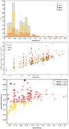 |
Fig. 1. Top: Number of sources per redshift. The bin size is 0.1. Middle: Radio luminosity at 1.4 GHz versus redshift. The redshift plotted is that of the galaxy groups. The radio luminosity is calculated from the 1.4 GHz flux density for the redshift of the object. Black represents all group galaxies, red is for BGGs, and yellow is for SGs (see Sect. 2 for clarification on the classification). Bottom: Halo mass versus redshift. Pink filled squares denote log10(M200/M⊙) > 13.5 and yellow open circles log10(M200/M⊙) < 13.5, which we refer to as log10(M200/M⊙)≈13.3 in the rest of the paper. The divide shows our adopted halo mass cut to account for sample completeness (Sect. 2.2). |
2.3. Sample of group galaxies used in this analysis
To analyse the radio luminosity function of group galaxies in COSMOS, we cross-matched the galaxy group catalogue and the 3 GHz VLA-COSMOS data (Smolčić et al. 2017a) within a 0.8″ radius. We furthermore used the 3 GHz VLA-COSMOS data presented by Novak et al. (2018), who constructed RLFs up to z ∼ 5.5, to compare to the total RLF in COSMOS up to z ∼ 2.3. Additionally, Novak et al. (2018) separated objects in SFGs and AGN following the radio excess prescription of Delvecchio et al. (2017). This method is based on the excess radio emission expected from star formation alone. Delvecchio et al. (2017) fitted the infrared spectral energy distribution of radio sources at 3 GHz VLA-COSMOS and calculated the contribution of the 3 GHz VLA-COSMOS radio sources to the radio luminosity by applying a conservative cut. Galaxies that exhibit an excess in radio emission above 3σ from what is expected from SF alone were deemed AGN, with the rest being SFGs. This method was used to separate the Novak et al. (2018) sample, which we use here for comparison, in SFGs and AGN. Finally, Novak et al. (2018) described possible biases and uncertainties associated with the data sample selection, and thus we refer the reader to this reference.
3. Methods and analysis
We describe the process of calculating the RLF for galaxies in groups in COSMOS (Gozaliasl et al. 2019) using the VLA-COSMOS 3 GHz data. We applied a cut in group mass, M200c > 1013.5 M⊙, to account for a difference in the limiting mass of the group catalogue with redshift (Sect. 2.2). This cut is demonstrated in the bottom frame of Fig. 1. We further separated group galaxies into BGGs and SGs. We compared the RLF of the population of SFGs and AGN at 3 GHz VLA-COSMOS in the same redshift bins to the total RLF calculated from the 3 GHz data (Novak et al. 2017; Smolčić et al. 2017a). We fitted linear and power-law models to the RLFs of GGs and compare them to the total RLF to obtain the contribution of GGs to the total RLF at 3 GHz VLA-COSMOS, something that has not been shown before in COSMOS.
3.1. Measuring the radio luminosity function
To obtain the total RLFs for GGs, SFGs, and AGN, we followed the method adopted by Novak et al. (2017) (see their Sect. 3.1). They computed the maximum observable volume Vmax, for each source (Schmidt 1968) and simultaneously applied completeness corrections that take into account the nonuniform rms noise and the resolution bias (see Sect. 3.1 in Novak et al. 2017). Then, the RLF is
 (1)
(1)
where L is the rest-frame luminosity at 1.4 GHz, derived using the radio spectral index of a source calculated between 1.4 GHz (Schinnerer et al. 2010) and 3 GHz (Smolčić et al. 2017a), and Δlog L is the width of the luminosity bin. The radio spectral index should remain unchanged between frequencies and is only available for a quarter of the 3 GHz VLA-COSMOS sample. For the rest of the sources detected only at 3 GHz, we assumed α = 0.7. The latter corresponds to the average spectral index of the entire 3 GHz population (see Sect. 4 in Smolčić et al. 2017a). Vmax is the maximum observable volume given by
![Mathematical equation: $$ \begin{aligned} V_{\mathrm{max},i} = \sum _{z=z_{\rm min}}^{z_{\rm max}} [V(z + \Delta z) - V(z)] C(z), \end{aligned} $$](/articles/aa/full_html/2025/01/aa43713-22/aa43713-22-eq2.gif) (2)
(2)
where the sum starts at zmin and adds co-moving spherical shells of volume ΔV = V(z + Δz)−V(z) in small redshift steps Δz = 0.01 until zmax. C(z) is the redshift-dependent geometrical and statistical correction factor. This takes into account sample incompleteness. For a thorough description of the biases, see Section 6.4 in Novak et al. (2017). The correction factor is given by
 (3)
(3)
where Aobs = 1.77 deg2 is the effective unflagged area observed in the optical-to-NIR wavelengths, Cradio is the completeness of the radio catalogue as a function of the flux density S3 GHz, and Copt is the completeness owing to radio sources without an assigned optical-NIR counterpart. Completeness corrections are shown in Smolčić et al. (2017a) in their Fig. 16 and Table 2, and in Novak et al. (2017) in their Fig. 2.
The redshift bins are large enough not to be severely affected by photometric redshift uncertainty and follow the selection of Novak et al. (2017) to allow comparisons. Luminosity bins in each redshift bin span the data’s observed luminosity range. To eliminate possible issues due to poorer sampling, the lowest luminosity ranges from the faintest observed source to the 5σ detection threshold at the upper redshift limit (corresponding to 5 × 2.3 μJy beam−1 at 3 GHz). The reported luminosity for each RLF is the median luminosity of the sources within the bin. The RLFs for all group galaxies are shown in Figs. 2 and 3 (black points) and are also listed in Table A.2. The RLFs for the BGGs and SGs are also shown in Figs. 2 and 3 (red squares/yellow stars) and are listed in Tables A.3 and A.4, respectively. The z bins in Figs. 2 and 3 are split in two halo mass M200c bins, above and below 1013.5 M⊙, and for our further analysis, we used the values above. We note that at 1.6 < z < 2.3 we do not have SGs above our halo-mass cut (M200c > 1013.5 M⊙). This is related to limits in the radio power that are probed at those redshifts, leading to low statistics and a scarcity of less massive groups. As discussed in Novak et al. (2018), there is only a 5−10% loss of completeness on the optical/NIR counterparts above z ∼ 2.
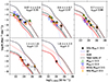 |
Fig. 2. Total radio luminosity functions of galaxies in groups. Black points indicate the RLFs for galaxy groups GGs derived using the Vmax method (see Sect. 3.1). Red squares and yellow stars mark the brightest group galaxies and satellites, respectively. The blue and red shaded areas show the ±3σ ranges of the best-fit evolution for the individual SFG and AGN populations, respectively (outlined in Section 3.2). The black dashed line is the fit to the total RLF at 3 GHz VLA-COSMOS (Novak et al. 2017; Smolčić et al. 2017c). For the z < 1 sub-samples (z < 0.4), the halos are split into massive (M200c > 1013.5 M⊙) and low-mass halos (M200c ≈ 1013.3 M⊙); the latter are shown for completion but not used in the analysis. For the rest of the redshift bins, all samples have M200c > 1013.5 M⊙. A halo mass cut, M200c > 1013.5 M⊙, was applied to the GGs, BGGs, and SGs. The solid black line is the scaled fit to the group galaxies’ RLFs, and the red solid line is the scaled fit for BGGs, as explained in Section 3.3.1. The scaled fit can be found in Fig. 2, and we do not show it here for SGs for clarity. The black line for the scaled fit for GGs in the last redshift bin is hidden by the red line for BGGs, because there are no SGs in that bin. |
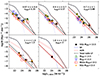 |
Fig. 3. Same as Fig. 2, but for the power-law fit. Total radio luminosity functions of galaxies in groups. Black points indicate the RLFs for GGs derived using the Vmax method (see Section 3.1). Red squares and yellow stars mark the brightest GGs and satellites, respectively. The blue and red shaded areas show the ±3σ ranges of the best-fit evolution for the individual SFG and AGN populations, respectively (outlined in Section 3.2). The black dashed line is the fit to the total RLF at 3 GHz VLA-COSMOS (Novak et al. 2017; Smolčić et al. 2017c). For the z < 1 subsamples (z < 0.4), the halos have been split into massive (M200c > 1013.5 M⊙) and low-mass halos (M200c ≈ 1013.3 M⊙); the latter are shown for completion but not used in the analysis. For the rest of the redshift bins, all samples have M200c > 1013.5 M⊙. A halo mass cut, M200c > 1013.5 M⊙, was applied to the GGs, BGGs, and SGs. The black solid line is the fit to the GGs’ RLF, and the red solid line is the best fit for BGGs, as explained in Section 3.3.2. We do not show the best fit for SGs for clarity. The black line for the linear regression fit for GGs in the last redshift bin is hidden by the red line for BGGs, because there are no SGs in that bin. |
3.2. The total RLF at 3 GHz VLA-COSMOS
We used the total RLF derived from the SFG and AGN populations at 3 GHz VLA-COSMOS (Novak et al. 2017, 2018; Smolčić et al. 2017c) to compare to the RLF values derived for the group galaxies in COSMOS. The RLFs of the SFG and AGN populations are calculated similarly for the same redshift bins as those described above and for the same area coverage as the galaxy groups in COSMOS. To fit the RLF, two models are used in the literature (e.g. Condon 1984; Sadler et al. 2002; Gruppioni et al. 2013): the pure luminosity evolution (PLE) and the pure density evolution (PDE). The RLF is fit, assuming its shape remains unchanged at all observed cosmic times. Only the position of the turnover and normalisation can change with redshift. This corresponds to the translation of the local LF in the log L − logΦ plane (Condon 1984) and can be divided into pure luminosity evolution (horizontal shift) and pure density evolution (vertical shift).
To describe an RLF across cosmic time, the local RLF is evolved in luminosity or density, or both (e.g. Condon 1984). This is parametrised (Novak et al. 2018) using two free parameters for density evolution (αD, βD), and two for luminosity evolution (αL, βL) to obtain
 (4)
(4)
where Φ0 is the local RLF. Since the shape and evolution of the RLF depend on the galaxy population type, Novak et al. (2017) used a power-law plus log-normal shape of the local RLF for SFGs. They used the combined data from Condon et al. (2002), Best et al. (2005), and Mauch & Sadler (2007) to obtain the best fit for the local value:
![Mathematical equation: $$ \begin{aligned} \Phi _0^{\mathrm{SF}}(L) = \Phi _\star \left(\frac{L}{L_\star }\right)^{1-\alpha } \exp \left[-\frac{1}{2\sigma ^2}\log ^2\left(1+\frac{L}{L_\star }\right)\right], \end{aligned} $$](/articles/aa/full_html/2025/01/aa43713-22/aa43713-22-eq5.gif) (5)
(5)
where Φ⋆ = 3.55 × 10⁻³ Mpc−3 dex−1, L⋆ = 1.85 × 10²¹ W Hz−1, α = 1.22, and σ = 0.63.
It was noted by Novak et al. (2017) that the PDE of SF galaxies would push the densities to very high numbers, thus making them inconsistent with the observed cosmic star formation rate densities. This is a consequence of the fact that our data can only constrain the bright, log-normal part of the SF RLF. For AGN, it was shown by Smolčić et al. (2017c) that the PDE and PLE models are similar, mostly because the shape of the RLF does not deviate strongly from a simple power law at the observed luminosities. Considering the above reasoning, while also trying to keep the parameter space degeneracy to a minimum, we decided to only use the PLE for our analysis. Thus, we adopted the approach of Novak et al. (2018), who fitted the total RLF for SFG and AGN populations by constructing a four–parameter redshift-dependent, pure-luminosity evolution model with two parameters for the SFG and AGN populations of the following form:
 (6)
(6)
where  is the local RLF for SFGs as in Eq. (5); for the nonlocal Universet it is a function of the quantity in parentheses, namely
  .
.  is the local RLF for AGN of the following form:
 (7)
(7)
where  , L⋆ = 1024.59 W Hz−1, α = −1.27, and β = −0.49 (Smolčić et al. 2017c; Mauch & Sadler 2007); for the nonlocal Universe it is a function of the quantity
  .
.
Novak et al. (2018) used the Markov chain Monte Carlo (MCMC) algorithm, available in the Python package EMCEE (Foreman-Mackey et al. 2013), to perform a multivariate fit to the data. The redshift dependence of the total evolution parameter α + z ⋅ β (see Eq. (6)) is necessary to describe the observations at all redshifts. The best-fit values for SFGs, based on the results of Novak et al. (2018), are  and
and  , and for AGN are
  and
and  . The αL and βL values for both SFGs and AGN are valid for z < 5.5 and within the redshift range of our sample of group galaxies. We used these values to plot the fit to the RLF for SFGs and AGN in Fig. 3, shown with blue and red lines, respectively. The total RLF (including all SFGs and AGN) is shown as a dashed black line in Fig. 3.
3.3. Fitting the RLF of group galaxies and comparing to the total 3 GHz RLF
Fitting the GG RLF is not a simple task. Performing an MCMC fit to the GG data with four free parameters (αSF, βSF, αAGN, and βAGN), similarly to what was done in Novak et al. (2018), is proven to be problematic, and the MCMC does not converge. Below, we investigate whether the functional form of the RLF, as presented above, can fit the GG RLF.
3.3.1. Scaled fit
We scaled the total 3 GHz RLF to fit the GG RLF using a MCMC method. The resulting GG RLF is shown in Fig. 2. There is a large deviation in the RLF values of GGs compared to the scaled fit, especially above luminosities of 1026 W Hz−1. We performed a χ2 test for the goodness of the fit between the GG values and the predicted scaled fit. The results are shown in Table A.9 in the appendix. The χ2 is large for most redshift bins, suggesting the model is not a good fit to the data. Additionally, we plot the ratio between data and model (see Fig. 4). It is evident that for the redshift bins with zmed = 0.35 and 1.2 the model under-fits the data in the high-luminosity bins by up to ∼2 orders of magnitude, suggesting that the functional form of the RLF does not work well in the case of group galaxies. Hence, we explored an alternative method for fitting the GG RLF.
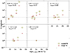 |
Fig. 4. Ratio of Φ GG RLF data points in adopted luminosity range and in each redshift bin, and the corresponding model value. Open olive circles denote the scaled fit method (Sect. 3.3.1) and brown crosses denote the linear-regression fit method (Sect. 3.3.2). The dotted gray line shows a perfect agreement between data and model. |
3.3.2. Power-law fit
We fitted a power law (linear regression fit in log-log) to the radio luminosity function of the group galaxies and, separately, of the BGGs and SGs, from redshifts 0.07 to 2.3 of the following form:
 (8)
(8)
where L⋆ is arbitrarily chosen to be 1024 W Hz−1, and Φ⋆ is the density at L⋆. Table A.5 shows the results for each fit. The best-fit model for the GGs is shown in Fig. 3, where we also compare the radio luminosity function of group galaxies to the total radio luminosity function of radio galaxies in the 3 GHz VLA-COSMOS survey and the radio luminosity function of AGN and the star-forming population. We also present the linear regression fit for BGGs, but exclude the one for SGs for clarity. The radio emission due to the star formation outweighs that from the AGN in lower redshifts, i.e., at z < 1, except at high-radio-luminosity bins where the AGN contribution dominates. This behaviour has been described in Novak et al. (2017) and Smolčić et al. (2017a), and agrees with other surveys. Adopting a fit similar to the total RLF used in Novak et al. (2018) provides a very poor fit to the GG data, particularly in the high-luminosity bins. Similarly, allowing both luminosity and Φ* to be free parameters resulted in the slope fit being dominated by two points with the smallest error. These tell us the GGs do not necessarily follow the shape of the total 3 GHz RLF, particularly at high luminosities, where we see increased radio activity of GG member galaxies.
3.3.3. Methods comparison
To investigate which method fits the GG RLF best, we compared the predicted to the real values. As mentioned earlier, we performed a χ2 test for the goodness of the fit between the GG values and the predicted ones (Table A.9). The test yields similar results for both methods, where the linear regression fit gives slightly better results, but neither of the models is a good fit to the data.
Furthermore, we visually inspect the RLF grid plots in Figs. 2 and 3. Both methods provide fairly good fits to the data. Should we use these fit lines to predict a value, it would not necessarily agree with the observed values in some areas of the parameter space. In particular, as seen in Fig. 2 for the scaled RLF, it does not fit the GGs above a radio luminosity of 1025 W Hz−1 well in all redshift bins, i.e. the part that can be dominated by AGN contribution (based on the 3 GHz RLF). In Fig. 3, for the power-law RLF, we also see the fit is not good for GGs above radio luminosity 1025 W Hz−1, but this is mainly in the redshift bins z ∼ 0.35 and z ∼ 1.2. From the ratio between data and model in Fig. 4, we see that the linear regression fit deviates less, on average, than the scaled fit from the observational data at all luminosities and redshifts.
To sum up, the χ2 test suggests neither of the fitting methods fits the data well. By visual inspection and from the ratio between data and model (Fig. 4), we see that we under-fit the GG RLF when using either of the two fitting methods for radio luminosities above 1025 W Hz−1 in the redshift bins zmed = 0.35 and 1.2. Below this value, there is a good rough agreement, with marginally better fits for the power-law RLF. The ratio between data and model in Fig. 4 aids us in selecting a method, i.e. the power-law, linear-regression fit. Thus, for the remainder of this analysis, we used the power-law fit method, but also present results of the scaled method for completeness (see Table A.6).
3.3.4. GG contribution to the total RLF
We calculate fractions obtained by the different methods we examined, the fraction of GG RLF to the total RLF if we apply the power-law, linear-regression fit (Sect. 3.3.2) and the fraction of GG RLF to the total RLF if we apply the scaled RFL (Sect. 3.3.1).
To quantify the contribution of the RLF of group galaxies to the total RLF of the 3 GHz population, we divide the power-law RLF of GGs, assuming a fixed slope of γ = −0.75, with the total RLF from the 3 GHz sample for each redshift bin. This gives the fractional contribution of group galaxies to the total RLF. In the top panel of Fig. 5, we plot the fraction with respect to the radio luminosity at 1.4 GHz up to 1025 W Hz−1. The reason for that is the RLF of 3 GHz VLA-COSMOS observations is not well constrained above that luminosity (Novak et al. 2018). Furthermore, we should consider that our model might be a good representation of the universe at L > 1025 W Hz−1, and the COSMOS is not suited for low-z studies due to the small volume coverage at low redshifts. Because of the different total RLF shapes per redshift bin, there is a bump in the curve, as expected. Using a fixed slope of γ = −0.75 does not impact our calculations as the value is within the errors for the fitted γ values presented in Table A.5.
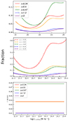 |
Fig. 5. Top: Fraction for group galaxies showing their contribution to the total 3 GHz radio-luminosity function at different epochs using the power-law, linear-regression fit method presented in Sect. 3.3.2 versus radio luminosity at 1.4 GHz. Colours represent different redshift bins. Middle: Same as above, but for all massive galaxies (M* > 1011.2 M⊙) with radio emission at 3 GHz (Smolčić et al. 2017b; Laigle et al. 2016). Bottom: Fraction using scaled fit method presented in Sect. 3.3.1. A halo mass cut above 1013.5 M⊙ was applied to all plots. |
We also calculated the RLFs of all massive galaxies with M* > 1011.2 M⊙, which are 3 GHz sources, and compared them to the total RLF. This fraction is shown in the middle panel of Fig. 5. We see an increase in the contribution to the total RLF at zmed = 0.3, and at higher redshifts it is similar to that of GGs. The choice of this stellar-mass cut, as a comparison, was motivated by the study of Smolčić et al. (2017c) in order to select massive galaxies across all redshifts. We discuss this further in the next section.
The bottom panel of Fig. 5 presents fractions using the scaled fit method presented in Sect. 3.3.1. The fraction is the same across the adopted luminosity range, as expected for a scaled fit. In Fig. 6, we plot the radio luminosity function and the fraction, for the scaled and power-law fits, in relation to redshift for the GGs, BGG, and SGs, and discuss this in the following section.
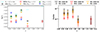 |
Fig. 6. Left: Radio luminosity function versus redshift for the group galaxies (black circles), brightest group galaxies BGGs (red squares), and satellite galaxies SGs (yellow stars). Cyan lines show the Φ* values at log |
4. Evolution of the RLF in galaxy groups
The top panel of Fig. 5 shows that the contribution of GGs to the total RLF increases from z ∼ 2 to 0.07, in particular for objects above radio luminosities at 1023 W Hz−1. This picture suggests an evolutionary scenario for the RLF of galaxy groups. We investigated this further by plotting the RLF of GGs, BGGs, and SGs (left panel) in Fig. 6, as well as their relative contribution to the total 3 GHz RLF as a function of redshift (right panel). The GG RLF has a low value at ∼2 down to z ∼ 1.25, followed by a sharp increase in the GG RLF at z ∼ 1 by a factor of six. After this, there is a smooth decline, mimicking a mild evolution by a factor of two. This is an interesting trend, which is not observed in the total RLF. As seen by the normalisation value of the total Φ* for a fixed radio luminosity at 1024 W Hz−1 (shown in cyan), galaxies in the 3 GHz sample display a decrease in their RLF with redshift across all redshifts, while the RLF of GGs increases at z ∼ 1 (left panel of Fig. 6); the peak at zmed ∼ 0.9 coincides with known overdensities in the COSMOS field. Interestingly, Smolčić et al. (2017c) showed that a similar trend can be reproduced with galaxies. In their Fig. 1, they present a slight increase in the median values of M* in their radio excess sample up to redshift z = 1, and the depletion of massive galaxies above z > 1, which we also see in the X-ray groups. We observed this at a median value of ∼1011.2 M⊙. In the middle panel of Fig. 5, we see that massive galaxies above 1011.2 M⊙ contribute a large fraction to the total 3 GHz RLF below z < 1. This suggests that not all massive galaxies are in groups, but those that are remain radioactive (Fig. 5). The GG contribution to the RLF shows a nearly flat, but slightly enhanced, behaviour below z < 0.75, while the GGs’ RLF does not exhibit a large contribution of radio emission at the lowest redshift bin as the massive galaxies’ RLF does. This suggests those massive galaxies are either in the field or occupy halo masses below our adopted cut at log10(M200c/M⊙) > 13.5.
The RLF of SGs dominates the RLF of group galaxies up to a redshift of zmed ∼ 1.2, with overdensities below z = 1 (Fig. 6–right). The fraction for the linear-regression fit method is a range of values that correspond to the adopted luminosity range (see also Fig. 5), plotted as violin plots. Both fractions follow the mild evolutionary trend we observe in the left panel. Scoville et al. (2013) studied the large-scale structure (LSS) in COSMOS and also report a statistically significant overdensity at z = 0.93. Additionally, the strongest density peaks, where we have massive clusters in COSMOS, are at redshifts 0.37, 0.73, and 0.83. Our 0.4 < z < 0.7 bin misses LSS on both ends. Above z ∼ 2 we do not currently have enough SGs to perform a robust analysis. This is likely to improve with future observations. The relative contribution of the SGs to the RLF of group galaxies is higher by a factor of two than that of BGGs below z ∼ 1. Additionally, BGGs contribute a small amount to the RLF of GGs, as seen in the left panel of Fig. 6, despite them being the most massive galaxies of the group. This is a very interesting result highlighting the importance of identifying the member group galaxies within a group and the need for high-sensitivity and high-resolution observations.
For reference, we split the redshift bins into low- and high-halo-mass objects. Objects with group masses below 1013.5 M⊙ contribute significantly to the lowest redshift bins and are linked to SGs, but this contribution was not taken into account in our analysis in order to ensure our sample is complete (see Sect. 2). The low-halo-mass points (Table A.5 and Fig. 3) show a faster turnover as we do not expect to detect many low-mass, high-luminosity objects.
Yuan et al. (2016), who studied BCGs, found that RLFs of 7138 BCGs in the 0.05 < z < 0.45 range do not show significant evolution with redshift. This no-evolution pattern of BCGs agrees with our results for BGGs in COSMOS. In the left panel of Fig. 6, we see that the RLF of BGGs fluctuates slightly with redshift, but it is the RLF of satellites that drives the redshift evolution.
Novak et al. (2018) discussed possible biases that could affect the calculations. These include the assumed shape of the radio SED being a power law and the radio excess criterion being too conservative and thus excluding low-luminosity AGN from the sample. We refer the reader to their discussion (see their Section 3.4). Furthermore, Novak et al. (2018) discussed possible biases that affect the RLF of the high-luminosity bin, i.e., bright radio but faint in the near-infrared sources (K = 24.5 mag). We constrained our sample to halo masses above 1013.5 M⊙ in order to perform an unbiased analysis. Incidentally, after the halo-mass cut, the remaining group galaxies in our sample are brighter than K = 24.5 mag.
In summary, we observe a nearly flat, but slightly enhanced, behaviour of the contribution of X-ray galaxy groups to the 3 GHz RLF up to z ∼ 0.75, driven by SGs and AGN (see Sect. 5) in GGs; this is followed by an increase and then a sharp drop. This agrees with past studies of the COSMOS field, and in particular with the study of Hale et al. (2018), who in their Fig. 10 showed that the AGN bias starts to deviate from values close to 5 × 10¹³ M⊙ at z < 1 toward 1 × 10¹³ M⊙ at z > 1. This explains the sharp drop we observe at z > 1, since we are probing halo masses > 1013.5 M⊙ (see bottom panel of Fig. 1).
5. The AGN and SFG contribution to the GG RLF
The group galaxy population has a mixture of contributions from AGN and SFGs. To explore how much these populations contribute to the GG RLF, we cross-correlated the X-ray galaxy group catalogue with the sample of Vardoulaki et al. (2021), which is a value-added catalogue at 3 GHz VLA-COSMOS, and it includes 130 FR-type radio sources (FRI, FRII; Fanaroff & Riley 1974, and hybrids FRI/FRII), 1818 jet-less compact radio AGN (COM AGN), and 7232 SFGs (see Table 1). Radio AGN in the Smolčić et al. (2017b) sample were selected on the basis of their radio excess, as mentioned above. This criterion, due to the 3σ cut applied, excludes several FR-type radio AGN, which were identified in Vardoulaki et al. (2021) and classified as radio AGN because they exhibit jets/lobes. SFGs are objects that do not display radio excess.
AGN and SFGs inside X-ray galaxy groups. Data from (Vardoulaki et al. 2021), cross-correlated with the X-ray galaxy group catalogue (Gozaliasl et al. 2019, and in prep.).
To separately quantify the contribution of these populations to the group RLF and to the total RLF, we calculated their RLFs as described in Sect. 3, using the Vmax method. All AGN and SFGs are in groups with halo masses of M200c > 1013.5 M⊙. The results for the AGN and SFG populations inside galaxy groups are shown in Fig. 7, where we also plot the RLF of AGN and SFGs from the sample of Novak et al. (2018), as in Fig. 3, and the total RLF at 3 GHz. In order to compare the RLF of AGN and SFGs that are GGs and the total RLF, we followed the analysis in Sect. 3.3.2. We fitted a linear regression and normalised it to 1024 W Hz−1 by applying Eq. (8) for γ = −0.75. The results are shown in Fig. 7.
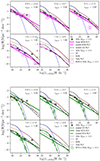 |
Fig. 7. Total radio luminosity functions of galaxies in groups, as in Figs. 2 and 3, including RLFs for different populations: radio AGN inside galaxy groups as magenta hexagons (top) and SFGs inside galaxy groups as green stars (bottom). To compare to the GG sample, we normalised the fit to the AGN and SFGs inside groups to L1.4 GHz = 1024 W Hz−1 and normalised a slope of γ = −0.75. For comparison, we show the GG sample (black circles for data, and a black solid line with a slope γ = −0.75 for the fit). We also plot the scaled AGN and SFG RLF (dashed-dotted lines), as reference. The red solid line shows the RLF for all AGN, the blue solid line shows it for all SFGs, and the dotted black line is the total RLF. A halo mass cut of M200c > 1013.5 M⊙ was applied. We note that the green solid line at the last bin of the SFG sample is forced to go though the two green stars. |
For completeness and to enable comparisons between the methods, we also present the scaled AGN and SFG parts of the total RLF to the GG data and overplot it in Fig. 7. In Table 2, we give the scaling coefficients used in Fig. 2 at the five redshift bins (separately for the AGN and SFG scaled fits). Visually, we see that the scaled RLF is not a good fit to the SFG at z < 0.4 and to the AGN at z < 1.6, inside X-ray galaxy groups. We performed a χ2 test for the AGN and SFGs, at all redshift bins, and present the results in Table A.9. The results show that neither of the fitting methods fits the data well.
Scaling coefficients for functional form of RLF (scaled fit) for AGN and SFG populations.
We further calculated and plot the fractional contribution of AGN and SFGs that lie inside groups to the total RLF at 3 GHz (Fig. 8) by replicating Fig. 5. The fraction was calculated by dividing the RLF of AGN and of SFGs inside galaxy groups by the total 3 GHz RLF. The fractions per redshift bin are curved lines due to the total RLF being curved. We find that there is a significant contribution from group AGN and SFGs at redshifts z < 1.6, and very little contribution above that. We present the values for these fractions in Table 3. For completeness, we calculated the fractional contribution of the AGN and SFG RLF to the GG and total RLFs in the case where the scaled fit method is used. The fractions are also presented in Table 1. In Fig. 8, we overplot the fraction of AGN and SFG RLFs to the GG RLF, where both RLFs were calculated using the scaled fit method. The respective lines follow the scaled AGN and SFG distributions, where AGN contribute more to the total RLF at higher luminosities, while SFGs dominate at lower luminosities. We stress that the scaled method for AGN and SFGs inside galaxy groups in COSMOS, and given the current dataset, is an approximation. It assumes the total 3 GHz RLF fits the subpopulations of AGN and SFGs inside galaxy groups. The reason for using a scaled fit is the smaller numbers of objects in galaxy groups compared to the total 3 GHz sample. Ideally, with a larger sample of AGN and SFGs inside groups, an MCMC procedure can provide a good fit to the subpopulations. Our analysis suggests that the total 3 GHz RLF is not a good fit for individual populations inside galaxy groups and that the picture is more complicated than that.
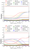 |
Fig. 8. Fractional contribution to total radio luminosity function at different epochs versus radio luminosity at 1.4 GHz for GGs (solid lines as in Fig. 5) and for different populations (dotted lines): AGN (top; labelled AGN v tot) and SFGs (bottom; labelled SFG v tot). Dotted-dashed lines show the fractional contribution of an AGN (labelled AGN v GG) and SFG (labelled SFG v GG) to the GG RLF. For reference, we plot the fraction of scaled AGN RLF (top) and scaled SFG RLF (bottom) to scaled GG RLF with dashed lines. Different colours represent different redshift bins as in Fig. 5. A halo mass cut of M200c > 1013.5 M⊙ was applied. |

For the linear-regression fit method, we obtain a constant value across all luminosities in Fig. 8 because the divided fits are both linear. The contribution of AGN RLF to the GG RLF is significant at the redshift bin zmed = 0.6 of around 56% and at zmed = 0.8 with fraction around 33%, and dominates the GG RLF. The fraction in SFGs is around 20% for zmed = 0.6 and zmed = 0.8, while at zmed = 1.2 the SFGs are dominating the GG RLF, with a fraction of 52%. At zmed = 0.3 we also see enhanced contribution in both AGN and SFGs compared to the GG RLF. This can be explained by the linear regression fit being normalised to 1024 W Hz−1 and forced to have a slope of γ = −0.75. For z > 1.6, the contribution of SFGs to the GG RLF drops sharply and below 1%, while we do not have AGN above z > 1.6. These findings suggest that both AGN and SFGs contribute to the GG RLF, with the AGN contribution peaking around z ∼ 1.
There are 67 AGN associated with BGGs and 71 with SGs, as shown in Table 1. For SFGs, we obtain 47 BGGs and 193 SGs. Due to the small number of sources per bin, we cannot replicate Fig. 6 by splitting the AGN and SFGs’ RLF inside groups in BGGs and SGs and calculating their RLF. Fig. 6 suggests the evolution of the GG RLF is driven by satellites. Based on our results from Fig. 8, at the zmed = 0.3 redshift bin, the SG AGN or SFGs are responsible for the peak of the GG RLF, while at zmed = 0.8 the increase is mainly driven by AGN.
How much of the AGN contribution to the GG RLF comes from extended radio emission, given the capabilities of the 3 GHz VLA-COSMOS survey, is not easy to estimate due to sample size limitations. From Table 1, we see that ∼82% of AGN inside galaxy groups are jet-less AGN. However, in order to robustly answer this question we need to separate FRs and COM AGN inside groups and calculate their RLFs per redshift bin, as above, which we cannot do given the small number of FRs per redshift bin. To have an idea of how extended the FRs within the AGN sample are, we look at the linear projected sizes D of FRs in Vardoulaki et al. (2021). The sensitivity and resolution of the 3 GHz VLA-COSMOS survey are 2.3 μJy/beam and  , respectively. This means that we are able to resolve and disentangle structures of ∼6 kpc at z ∼ 2. The smallest FR reported in Vardoulaki et al. (2021) has D = 8.1 kpc at z = 2.467, just above the resolution limit, and the smallest edge-brightened FR has D = 24.3 kpc at z = 1.128, where the lobes are separated by 8 kpc. Inside X-ray galaxy groups, the smallest FR has D = 13.37 kpc at z = 0.38 with the most extended having D = 608.4 kpc and z = 1.168; this is also the most extended object in the Vardoulaki et al. (2021) FR sample. Future surveys with increased sensitivity and resolution will be able to resolve jets and lobes in AGN that appear compact at 3 GHz VLA-COSMOS. With future observations at larger sky areas and improved statistics, we will be in a better position to resolve this issue.
Nobels et al. (2022) showed, via hydrodynamical simulations of galaxy groups/clusters with masses above M200c > 1013.5 M⊙ (as the ones studied here), a cyclical behaviour of AGN quenching and star formation activity: long periods where star formation is quenched by the AGN are followed by shorter periods of star formation and black hole accretion. This is because the reduction of AGN feedback makes the ICM unstable to precipitation and thus initiating a new episode of intense star formation. Furthermore, Pasini et al. (2020) reported that feedback mechanisms in groups and clusters of galaxies are similar. In our study, we find that the AGN contribution to the galaxy group’s RLF dominates at redshifts up to zmed = 0.8. The hosts of these AGN at 3 GHz VLA-COSMOS are quenched, based on the study of Vardoulaki et al. (2021). AGN at zmed = 0.8 show low star formation rates (SFRmed ∼ 8 M⊙/yr) compared to SFGs at similar redshifts (SFRmed ∼ 24 M⊙/yr). At lower redshifts (zmed = 0.3), both AGN and SFG populations show low median SFRs (∼1.2 and ∼3.4 M⊙/yr, respectively). The median SFR in the field shows similar median values compared to the one inside galaxy groups for zmed = 0.3 & 0.8, for both AGN and SFGs.
To verify the cyclical behaviour presented in Nobels et al. (2022), a study of the duty cycle of individual objects is needed, which is beyond the scope of this analysis. A thorough analysis comparing AGN and SFGs in relation to a large-scale environment is presented in Vardoulaki et al. (2021), and we refer the reader to that study. A detailed investigation of AGN feedback since z5 at 3 GHz COSMOS is presented in the studies of Smolčić et al. (2017c) and Ceraj et al. (2018).
Our analysis suggests that the bulk of high-z log10(M200c/M⊙) > 13.5 groups must have formed recently, and so the cooling has not been established. This is linked to the drop in occurrence of AGN in groups at high z by a factor of six, suggesting that AGN feedback is lower by a factor of six at high redshifts. Hence, AGN feedback in the groups we are studying (log10(M200c/M⊙) in the range 13.5−14.5) must be a recent phenomenon. There seems to be a change in the way groups operate above z > 1, with a faster evolution. Mass changes quickly, and there is not enough time to virialise. Due to the lack of virialisation, the cooling does not start, and the AGN activity is suppressed. This change can be triggered by (1) high thermalisation of matter, which is not sufficient in this case; or (2) dynamically young groups where gas cooling does not happen. On the other hand, low-mass groups form at z = 6. These are found to host radio AGN and have time to virialise, cool, and provide feedback. Additionally, cooling times for energetic electrons are much lower at high-z.
6. Summary and conclusions
We present a study of radio luminosity functions, RLFs, of group galaxies in the COSMOS field based on data from the VLA-COSMOS 3 GHz Large Project (Smolčić et al. 2017a) and the X-ray galaxy groups catalogue (Gozaliasl et al. 2019, and in prep.). The X-ray galaxy groups cover halo masses in the M200c = 8 × 10¹² − 3 × 10¹⁴ M⊙ range and the 0.07 < z < 2.3 redshift range. To probe the same group population at all redshifts, we applied a halo-mass cut and only selected groups with halo masses of M200c > 1013.5 M⊙. Furthermore, we applied completeness corrections to the calculation of the RLF (Novak et al. 2017), and all galaxy-group members are brighter than K = 24.5 mag, which allows for an unbiased analysis.
We calculated the RLF of group galaxies based on the Vmax method and compared it to the 3 GHz RLF from Novak et al. (2018), who fit the total RLF with pure-luminosity evolution models that depend on redshift. The AGN and SFG populations, characterised by the radio-excess parameter, were fit with an MCMC algorithm. We fitted the group galaxies’ (GGs) RLFs using two methods: (a) scaling the total 3 GHz RLF and (b) using a linear (power-law) fit and estimating the contribution to the total RLF. We also studied how much satellites (SGs), brightest group galaxies (BGGs), AGN, and SFGs contribute to the RLF of galaxy groups and to the total 3 GHz RLF. The two fitting methods provide similar results, with the ratio between data and model (Fig. 4) suggesting the power-law fit was slightly better for the GG RLF. The linear regression fit is the adopted method for the interpretation of the results.
Our main results are summarised below:
-
The relative contribution of the group galaxies to the total 3 GHz radio luminosity function in galaxies in the COSMOS field generally decreases with increasing redshift, from 4% at low z to 1% at z > 1, with an overdensity below z < 1; this is in line with large-scale structure studies of the COSMOS field.
-
The GG RLF has a low value at ∼2 down to z ∼ 1.25, followed by a sharp increase in the GG RLF at z ∼ 1 by a factor of six. This is followed by a smooth decline, which is driven mainly by satellite GGs. The latter suggests a mild evolution in the RLF of GGs from z ∼ 1 to 0.07 by a factor of three.
-
The RLF of SGs dominates the RLF of group galaxies up to a redshift of z ∼ 1.2, where we observe a drop in the RLF of both BGGs and SGs.
-
The AGN dominate the GG RLF at z ∼ 1, while the SFGs dominate the GG RLF at zmed = 1.2.
In summary, we observed a nearly flat, but enhanced, behaviour of the contribution of galaxy groups to the total 3 GHz RLF up to z ∼ 0.75, driven by SGs and AGN in GGs. This is followed by an increase and then a sharp drop, which agrees with the literature and is related to AGN occupying less massive halos above z > 1. The enhanced contribution and sharp drop are not driven by a possible sensitivity drop at high redshifts, but by the actual abundance of massive groups, which is enhanced in high-density peaks with regard to normal galaxies and creates an enhancement of the fractional contribution of radio galaxies. In a case where all the galaxies are groups of similar masses, but we detect only some with X-rays, the ratio would have stayed the same, independent of the density of the field.
Another important result of this analysis is the RLF itself for group galaxies, as well as the contribution of the satellites and BGGs in group environments, which is a major observational constraint for tuning the models. Our study provides an observational probe for the accuracy of the numerical predictions of the radio emission in galaxies in a group environment. Finally, our results show a drop in the occurrence of AGN in groups at high z by a factor of six, suggesting that AGN feedback is lower by a factor of six at high redshifts. The bulk of high-z log10(M200c/M⊙) > 13.5 groups must have been formed recently, and so the cooling has not been established. AGN at high-z occupy low-halo-mass systems (≈1013.3 M⊙), revealing the details on the processes accountable for the galaxy evolution in massive environments.
Data availability
Table A.1 is available at the CDS via anonymous ftp to cdsarc.cds.unistra.fr (130.79.128.5) or via https://cdsarc.cds.unistra.fr/viz-bin/cat/J/A+A/693/A61
Tables A.2–A.9 have been uploaded to Zenodo https://zenodo.org/records/14192888
Acknowledgments
We would like to thank Aritra Basu for useful discussions. We would like to thank the anonymous referee for a constructive report which significantly improved our manuscript. EV acknowledges support from Carl Zeiss Stiftung with the project code KODAR.
References
- Barr, J. M., Bremer, M. N., Baker, J. C., & Lehnert, M. D. 2003, MNRAS, 346, 229 [NASA ADS] [CrossRef] [Google Scholar]
- Best, P., Lehnert, M., Röttgering, H., & Miley, G. 2002, ASP Conf. Ser., 268, 19 [NASA ADS] [Google Scholar]
- Best, P. N., Kauffmann, G., Heckman, T. M., & Ivezić, Ž. 2005, MNRAS, 362, 9 [Google Scholar]
- Branchesi, M., Gioia, I. M., Fanti, C., Fanti, R., & Perley, R. 2006, A&A, 446, 97 [NASA ADS] [CrossRef] [EDP Sciences] [Google Scholar]
- Byrd, G., & Valtonen, M. 1990, ApJ, 350, 89 [NASA ADS] [CrossRef] [Google Scholar]
- Ceraj, L., Smolčić, V., Delvecchio, I., et al. 2018, A&A, 620, A192 [NASA ADS] [CrossRef] [EDP Sciences] [Google Scholar]
- Civano, F., Marchesi, S., Comastri, A., et al. 2016, ApJ, 819, 62 [Google Scholar]
- Clemens, M. S., Vega, O., Bressan, A., et al. 2008, A&A, 477, 95 [NASA ADS] [CrossRef] [EDP Sciences] [Google Scholar]
- Condon, J. J. 1984, ApJ, 287, 461 [Google Scholar]
- Condon, J. J. 1992, ARA&A, 30, 575 [Google Scholar]
- Condon, J. J., Cotton, W. D., & Broderick, J. J. 2002, AJ, 124, 675 [Google Scholar]
- Delvecchio, I., Smolčić, V., Zamorani, G., et al. 2017, A&A, 602, A3 [NASA ADS] [CrossRef] [EDP Sciences] [Google Scholar]
- Dressler, A. 1980, ApJ, 236, 351 [Google Scholar]
- Elvis, M., Civano, F., Vignali, C., et al. 2009, ApJS, 184, 158 [Google Scholar]
- Fanaroff, B. L., & Riley, J. M. 1974, MNRAS, 167, 31P [Google Scholar]
- Finoguenov, A., Guzzo, L., Hasinger, G., et al. 2007, ApJS, 172, 182 [Google Scholar]
- Foreman-Mackey, D., Hogg, D. W., Lang, D., & Goodman, J. 2013, PASP, 125, 306 [Google Scholar]
- George, M. R., Leauthaud, A., Bundy, K., et al. 2011, ApJ, 742, 125 [Google Scholar]
- Gozaliasl, G., Finoguenov, A., Tanaka, M., et al. 2019, MNRAS, 483, 3545 [Google Scholar]
- Gruppioni, C., Pozzi, F., Rodighiero, G., et al. 2013, MNRAS, 432, 23 [Google Scholar]
- Hale, C. L., Jarvis, M. J., Delvecchio, I., et al. 2018, MNRAS, 474, 4133 [NASA ADS] [CrossRef] [Google Scholar]
- Khosroshahi, H. G., Raouf, M., Miraghaei, H., et al. 2017, ApJ, 842, 81 [NASA ADS] [CrossRef] [Google Scholar]
- Laigle, C., McCracken, H. J., Ilbert, O., et al. 2016, ApJS, 224, 24 [Google Scholar]
- Larson, R. B. 1980, Phil. Trans. Roy. Soc. London Ser. A, 296, 299 [Google Scholar]
- Leauthaud, A., Finoguenov, A., Kneib, J.-P., et al. 2010, ApJ, 709, 97 [Google Scholar]
- Magorrian, J., Tremaine, S., Richstone, D., et al. 1998, AJ, 115, 2285 [Google Scholar]
- Mauch, T., & Sadler, E. M. 2007, MNRAS, 375, 931 [Google Scholar]
- Miller, N. A., & Owen, F. N. 2003, AJ, 125, 2427 [NASA ADS] [CrossRef] [Google Scholar]
- Nobels, F. S. J., Schaye, J., Schaller, M., Bahé, Y. M., & Chaikin, E. 2022, MNRAS, 515, 4838 [CrossRef] [Google Scholar]
- Novak, M., Smolčić, V., Delhaize, J., et al. 2017, A&A, 602, A5 [NASA ADS] [CrossRef] [EDP Sciences] [Google Scholar]
- Novak, M., Smolčić, V., Schinnerer, E., et al. 2018, A&A, 614, A47 [NASA ADS] [CrossRef] [EDP Sciences] [Google Scholar]
- Oemler, A. 1974, ApJ, 194, 1 [Google Scholar]
- Pasini, T., Brüggen, M., de Gasperin, F., et al. 2020, MNRAS, 497, 2163 [NASA ADS] [CrossRef] [Google Scholar]
- Raouf, M., Khosroshahi, H. G., Mamon, G. A., et al. 2018, ApJ, 863, 40 [NASA ADS] [CrossRef] [Google Scholar]
- Reddy, N. A., & Yun, M. S. 2004, ApJ, 600, 695 [NASA ADS] [CrossRef] [Google Scholar]
- Sadler, E. M., Jenkins, C. R., & Kotanyi, C. G. 1989, MNRAS, 240, 591 [NASA ADS] [Google Scholar]
- Sadler, E. M., Jackson, C. A., Cannon, R. D., et al. 2002, MNRAS, 329, 227 [Google Scholar]
- Schinnerer, E., Sargent, M. T., Bondi, M., et al. 2010, ApJS, 188, 384 [Google Scholar]
- Schmidt, M. 1968, ApJ, 151, 393 [Google Scholar]
- Scoville, N., Aussel, H., Brusa, M., et al. 2007, ApJS, 172, 1 [Google Scholar]
- Scoville, N., Arnouts, S., Aussel, H., et al. 2013, ApJS, 206, 3 [Google Scholar]
- Smolčić, V., Novak, M., Bondi, M., et al. 2017a, A&A, 602, A1 [Google Scholar]
- Smolčić, V., Delvecchio, I., Zamorani, G., et al. 2017b, A&A, 602, A2 [NASA ADS] [CrossRef] [EDP Sciences] [Google Scholar]
- Smolčić, V., Novak, M., Delvecchio, I., et al. 2017c, A&A, 602, A6 [NASA ADS] [CrossRef] [EDP Sciences] [Google Scholar]
- Tabatabaei, F. S., Schinnerer, E., Krause, M., et al. 2017, ApJ, 836, 185 [Google Scholar]
- Vardoulaki, E., Jiménez Andrade, E. F., Delvecchio, I., et al. 2021, A&A, 648, A102 [NASA ADS] [CrossRef] [EDP Sciences] [Google Scholar]
- Yuan, Z. S., Han, J. L., & Wen, Z. L. 2016, MNRAS, 460, 3669 [Google Scholar]
Appendix A: Numerical results from the calculation of the radio luminosity function in X-ray galaxy groups in COSMOS
Table A.1 is available via CDS and Tables A2-A9 are available in Zenodo.
Radio properties of Group Galaxies in COSMOS
Radio-luminosity functions of GGs obtained with the Vmax method. A halo mass cut, M200c > 1013.5 M⊙, was applied. We note that the error on Φ is in dex.
Radio-luminosity functions of BGGs obtained with the Vmax method. A halo mass cut, M200c > 1013.5 M⊙, was applied. We note that the error on Φ is in dex.
Radio-luminosity functions of satellites obtained with the Vmax method. A halo mass cut, M200c > 1013.5 M⊙, was applied. We note that the error on Φ is in dex.
Best power-law fit parameters. A halo mass cut, M200c > 1013.5 M⊙, was applied.
Φ* fits using the scaled method. A halo mass cut, M200c > 1013.5 M⊙, was applied.
Radio-luminosity functions of AGN inside X-ray GGs obtained with the Vmax method. A halo mass cut, M200c > 1013.5 M⊙, was applied. We note that the error on Φ is in dex.
Radio-luminosity functions of SFGs inside X-ray galaxy groups obtained with the Vmax method. A halo mass cut, M200c > 1013.5 M⊙, was applied. We note that the error on Φ is in dex.
χ2 test results for the GGs (Sect. 3.3.3) AGN, and SFGs (Sect. 5). PL is for the power-law, linear-regression fit, and SC is for the scaled fit. DoF denotes the degrees of freedom.
All Tables
AGN and SFGs inside X-ray galaxy groups. Data from (Vardoulaki et al. 2021), cross-correlated with the X-ray galaxy group catalogue (Gozaliasl et al. 2019, and in prep.).
Scaling coefficients for functional form of RLF (scaled fit) for AGN and SFG populations.
Radio-luminosity functions of GGs obtained with the Vmax method. A halo mass cut, M200c > 1013.5 M⊙, was applied. We note that the error on Φ is in dex.
Radio-luminosity functions of BGGs obtained with the Vmax method. A halo mass cut, M200c > 1013.5 M⊙, was applied. We note that the error on Φ is in dex.
Radio-luminosity functions of satellites obtained with the Vmax method. A halo mass cut, M200c > 1013.5 M⊙, was applied. We note that the error on Φ is in dex.
Best power-law fit parameters. A halo mass cut, M200c > 1013.5 M⊙, was applied.
Φ* fits using the scaled method. A halo mass cut, M200c > 1013.5 M⊙, was applied.
Radio-luminosity functions of AGN inside X-ray GGs obtained with the Vmax method. A halo mass cut, M200c > 1013.5 M⊙, was applied. We note that the error on Φ is in dex.
Radio-luminosity functions of SFGs inside X-ray galaxy groups obtained with the Vmax method. A halo mass cut, M200c > 1013.5 M⊙, was applied. We note that the error on Φ is in dex.
χ2 test results for the GGs (Sect. 3.3.3) AGN, and SFGs (Sect. 5). PL is for the power-law, linear-regression fit, and SC is for the scaled fit. DoF denotes the degrees of freedom.
All Figures
|
Fig. 1. Top: Number of sources per redshift. The bin size is 0.1. Middle: Radio luminosity at 1.4 GHz versus redshift. The redshift plotted is that of the galaxy groups. The radio luminosity is calculated from the 1.4 GHz flux density for the redshift of the object. Black represents all group galaxies, red is for BGGs, and yellow is for SGs (see Sect. 2 for clarification on the classification). Bottom: Halo mass versus redshift. Pink filled squares denote log10(M200/M⊙) > 13.5 and yellow open circles log10(M200/M⊙) < 13.5, which we refer to as log10(M200/M⊙)≈13.3 in the rest of the paper. The divide shows our adopted halo mass cut to account for sample completeness (Sect. 2.2). |
| In the text | |
|
Fig. 2. Total radio luminosity functions of galaxies in groups. Black points indicate the RLFs for galaxy groups GGs derived using the Vmax method (see Sect. 3.1). Red squares and yellow stars mark the brightest group galaxies and satellites, respectively. The blue and red shaded areas show the ±3σ ranges of the best-fit evolution for the individual SFG and AGN populations, respectively (outlined in Section 3.2). The black dashed line is the fit to the total RLF at 3 GHz VLA-COSMOS (Novak et al. 2017; Smolčić et al. 2017c). For the z < 1 sub-samples (z < 0.4), the halos are split into massive (M200c > 1013.5 M⊙) and low-mass halos (M200c ≈ 1013.3 M⊙); the latter are shown for completion but not used in the analysis. For the rest of the redshift bins, all samples have M200c > 1013.5 M⊙. A halo mass cut, M200c > 1013.5 M⊙, was applied to the GGs, BGGs, and SGs. The solid black line is the scaled fit to the group galaxies’ RLFs, and the red solid line is the scaled fit for BGGs, as explained in Section 3.3.1. The scaled fit can be found in Fig. 2, and we do not show it here for SGs for clarity. The black line for the scaled fit for GGs in the last redshift bin is hidden by the red line for BGGs, because there are no SGs in that bin. |
| In the text | |
|
Fig. 3. Same as Fig. 2, but for the power-law fit. Total radio luminosity functions of galaxies in groups. Black points indicate the RLFs for GGs derived using the Vmax method (see Section 3.1). Red squares and yellow stars mark the brightest GGs and satellites, respectively. The blue and red shaded areas show the ±3σ ranges of the best-fit evolution for the individual SFG and AGN populations, respectively (outlined in Section 3.2). The black dashed line is the fit to the total RLF at 3 GHz VLA-COSMOS (Novak et al. 2017; Smolčić et al. 2017c). For the z < 1 subsamples (z < 0.4), the halos have been split into massive (M200c > 1013.5 M⊙) and low-mass halos (M200c ≈ 1013.3 M⊙); the latter are shown for completion but not used in the analysis. For the rest of the redshift bins, all samples have M200c > 1013.5 M⊙. A halo mass cut, M200c > 1013.5 M⊙, was applied to the GGs, BGGs, and SGs. The black solid line is the fit to the GGs’ RLF, and the red solid line is the best fit for BGGs, as explained in Section 3.3.2. We do not show the best fit for SGs for clarity. The black line for the linear regression fit for GGs in the last redshift bin is hidden by the red line for BGGs, because there are no SGs in that bin. |
| In the text | |
|
Fig. 4. Ratio of Φ GG RLF data points in adopted luminosity range and in each redshift bin, and the corresponding model value. Open olive circles denote the scaled fit method (Sect. 3.3.1) and brown crosses denote the linear-regression fit method (Sect. 3.3.2). The dotted gray line shows a perfect agreement between data and model. |
| In the text | |
|
Fig. 5. Top: Fraction for group galaxies showing their contribution to the total 3 GHz radio-luminosity function at different epochs using the power-law, linear-regression fit method presented in Sect. 3.3.2 versus radio luminosity at 1.4 GHz. Colours represent different redshift bins. Middle: Same as above, but for all massive galaxies (M* > 1011.2 M⊙) with radio emission at 3 GHz (Smolčić et al. 2017b; Laigle et al. 2016). Bottom: Fraction using scaled fit method presented in Sect. 3.3.1. A halo mass cut above 1013.5 M⊙ was applied to all plots. |
| In the text | |
|
Fig. 6. Left: Radio luminosity function versus redshift for the group galaxies (black circles), brightest group galaxies BGGs (red squares), and satellite galaxies SGs (yellow stars). Cyan lines show the Φ* values at log |
| In the text | |
|
Fig. 7. Total radio luminosity functions of galaxies in groups, as in Figs. 2 and 3, including RLFs for different populations: radio AGN inside galaxy groups as magenta hexagons (top) and SFGs inside galaxy groups as green stars (bottom). To compare to the GG sample, we normalised the fit to the AGN and SFGs inside groups to L1.4 GHz = 1024 W Hz−1 and normalised a slope of γ = −0.75. For comparison, we show the GG sample (black circles for data, and a black solid line with a slope γ = −0.75 for the fit). We also plot the scaled AGN and SFG RLF (dashed-dotted lines), as reference. The red solid line shows the RLF for all AGN, the blue solid line shows it for all SFGs, and the dotted black line is the total RLF. A halo mass cut of M200c > 1013.5 M⊙ was applied. We note that the green solid line at the last bin of the SFG sample is forced to go though the two green stars. |
| In the text | |
|
Fig. 8. Fractional contribution to total radio luminosity function at different epochs versus radio luminosity at 1.4 GHz for GGs (solid lines as in Fig. 5) and for different populations (dotted lines): AGN (top; labelled AGN v tot) and SFGs (bottom; labelled SFG v tot). Dotted-dashed lines show the fractional contribution of an AGN (labelled AGN v GG) and SFG (labelled SFG v GG) to the GG RLF. For reference, we plot the fraction of scaled AGN RLF (top) and scaled SFG RLF (bottom) to scaled GG RLF with dashed lines. Different colours represent different redshift bins as in Fig. 5. A halo mass cut of M200c > 1013.5 M⊙ was applied. |
| In the text | |
Current usage metrics show cumulative count of Article Views (full-text article views including HTML views, PDF and ePub downloads, according to the available data) and Abstracts Views on Vision4Press platform.
Data correspond to usage on the plateform after 2015. The current usage metrics is available 48-96 hours after online publication and is updated daily on week days.
Initial download of the metrics may take a while.