| Issue |
A&A
Volume 694, February 2025
|
|
|---|---|---|
| Article Number | A261 | |
| Number of page(s) | 14 | |
| Section | Extragalactic astronomy | |
| DOI | https://doi.org/10.1051/0004-6361/202452954 | |
| Published online | 19 February 2025 | |
An empirical model of the extragalactic radio background
1
School of Astronomy and Space Science, Nanjing University, 163 Xianlin Avenue, Nanjing 210023, People’s Republic of China
2
Key Laboratory of Modern Astronomy and Astrophysics (Nanjing University), Ministry of Education, Nanjing 210023, People’s Republic of China
⋆ Corresponding author; This email address is being protected from spambots. You need JavaScript enabled to view it.
Received:
11
November
2024
Accepted:
10
December
2024
Abstract
Aims. Radio observations provide a powerful tool for constraining the assembly of galaxies over cosmic time. Recent deep and wide radio continuum surveys have significantly improved our understanding of the radio emission properties of active galactic nuclei (AGNs) and star-forming galaxies (SFGs) across 0 < z < 4. These findings have allowed us to derive an empirical model of the radio continuum emission of galaxies, based on their star formation rates and the probability of their hosting radio AGNs. In this work, we verify how well this empirical model can reproduce the extragalactic radio background (ERB), which can provide new insights into the contribution to the ERB from galaxies of different masses and redshfits.
Methods. We made use of the Empirical Galaxy Generator (EGG) code to generate a near-infrared (NIR) selected, flux-limited, multiwavelength catalog to mimic real observations. Then we assigned radio continuum flux densities to galaxies based on their star formation rates and the probability that they would host a radio-AGN of a specific 1.4 GHz luminosity. We also applied special treatments to reproduce the clustering signal of radio AGNs.
Results. Our empirical model successfully recovers the observed 1.4 GHz radio luminosity functions (RLFs) of both AGN and SFG populations, as well as the differential number counts at various radio bands. The uniqueness of this approach also allows us to directly link the radio flux densities of galaxies to other properties, including redshifts, stellar masses, and magnitudes at various photometric bands. We find that roughly half of the radio continuum sources to be detected by the Square Kilometer Array (SKA) at z ∼ 4 − 6 will be too faint to be detected in the optical survey (r ∼ 27.5) carried out by Rubin Observatory.
Conclusions. Unlike previous studies, which utilized (extrapolations of) RLFs to reproduce the ERB, our work starts from a simulated galaxy catalog with realistic physical properties. It has the potential to simultaneously and self-consistently reproduce physical properties of galaxies across a wide range of wavelengths, from the optical, NIR, and far-infrared (FIR) to radio wavelengths. Our empirical model can shed light on the contribution of different galaxies to the extragalactic background light and would greatly facilitate the design of future multiwavelength galaxy surveys.
Key words: galaxies: evolution / galaxies: luminosity function / mass function / galaxies: photometry / radio continuum: galaxies
© The Authors 2025
 Open Access article, published by EDP Sciences, under the terms of the Creative Commons Attribution License (https://creativecommons.org/licenses/by/4.0), which permits unrestricted use, distribution, and reproduction in any medium, provided the original work is properly cited.
This article is published in open access under the Subscribe to Open model. This email address is being protected from spambots. You need JavaScript enabled to view it. to support open access publication.
1. Introduction
Among the spectral windows that are not as severely affected by Earth’s atmosphere, radio observations are advantageous, given they operate at a wide range of frequencies and probe a wide range of redshifts. Therefore, radio observations serve as a powerful tool to constrain the growth and evolution of galaxies across the history of our Universe. Our knowledge regarding the extragalactic radio background has broadened thanks to multiple generations of radio surveys. It has been established that powerful radio sources are usually radio emission produced by accreting supermassive black holes (SMBHs), which are expected to be responsible for the regulation to their host galaxies (e.g., Croton et al. 2006). Meanwhile, less powerful radio sources are predominately star forming galaxies (SFGs), displaying a tight correlation between radio emission and star formation rates (SFRs). This knowledge is applied in many fields, for example, selecting radio active galactic nuclei (AGNs) according to the radio luminosity (see Tadhunter 2016, for a recent review) and using radio emission as a dust-invariant indicator of SFRs (e.g., Yun et al. 2001; Garn et al. 2009; Brown et al. 2017; Davies et al. 2017; Wang et al. 2019, among others).
Realistic simulations of extragalactic radio galaxies and images provide valuable support in many aspects, such as evaluating the performance of both “hardware” instruments and “software” source extraction pipelines. Popular mock radio source catalogs are mainly built upon (extrapolations of) radio luminosity functions (RLFs). As a straightforward measurement, the RLF reflects the abundance of radio sources within a certain luminosity range across a wide range of redshift. Therefore, it is convenient to directly calculate how many radio sources are expected to exist within a certain flux density range at any given redshift.
Via this method, current mock radio catalogs have succeeded in reproducing the extragalactic radio background (ERB) based on the RLFs of different populations. For example, the Square Kilometer Array (SKA) Design Study Simulated Skies simulation (S3; Wilman et al. 2008) produced mock radio sources based on observed RLFs of five distinct galaxy populations: radio-quiet AGNs, radio-loud AGNs composed of Fanaroff–Riley I (FRI) and Fanaroff–Riley II (FRII) sources, and SFGs composed of quiescent and star-bursting galaxies. A more recent work by The Tiered Radio Extragalactic Continuum Simulation (TRECS; Bonaldi et al. 2019) exploited RLF models developed in Massardi et al. (2010) and split radio-loud AGNs into three populations with different evolutionary properties: steep-spectrum sources (SS-AGNs), flat-spectrum radio quasars (FSRQs), and Bl Lacertae (BL Lacs). These mock radio catalogs prove to be successfully recover many observable quantities, such as RLFs and source number counts, at various frequencies. However, it is difficult to gain insights into other physical information of these radio sources, such as how quickly they form stars and how they shine at other wavelengths. This empirical method also tended to overlook the physical origins behind these scenarios; for example, how the fraction of radio AGNs evolve across cosmic time as well as how much the ERB contributes to radio AGNs and SFGs separately at given stellar mass.
With this issue in mind, we are aiming to recover the ERB not based on the observed RLFs, but based on a mock mass-complete galaxy catalog. It starts from fully-explored stellar mass functions and incorporates a rich store of information on the physical properties.
Over the past few decades, we have deepened our exploration of our Universe and established a comprehensive set of knowledge that brings us closer to the physical properties of galaxies, at least at 0 < z < 4. These properties include the redshift-dependent distribution of their stellar masses (e.g., Muzzin et al. 2013; Duncan et al. 2014; Tomczak et al. 2014; Davidzon et al. 2017, among many others) and SFRs (e.g., Noeske et al. 2007; Speagle et al. 2014; Schreiber et al. 2015; Pearson et al. 2018, among many others), as well as the spectral energy distributions (SEDs) of different populations across a wide range of spectrum (e.g., Dale & Helou 2002; Magdis et al. 2012; Conroy 2013, among many others). By utilizing these empirical knowledge, astronomers are able to generate mock galaxy catalogs, reproduce various observables in a self-consistent way, and extrapolate to much deeper depths. This allows us to predict what types of galaxies can be directly observed (e.g., SIDES simulation of far-infrared to submillimeter extragalactic background in Béthermin et al. (2017) and EGG code developed by Schreiber et al. (2017) used in this work). This method is also capable of creating mock galaxy catalogs at a fast speed, without inducing complex large-scale dark matter simulations, which are computationally expensive (Schreiber et al. 2017).
Thanks to this method, we are able to connect radio sources to their host galaxies with a plethora of physical information, enabling studying extragalactic radio sources in a multi-wavelength context and harnessing the power of combining different observational techniques.
The next-generation radio facility SKA is expected to revolutionize our current knowledge regarding finding fainter and farther radio sources with its supreme sensitivity and angular resolution. Prior to its final operation, it is necessary to assess how far it can surpass the current radio telescopes and what improvement it can bring when work in collaboration with other mainstream optical\near-infrared (NIR) large sky surveys such as Large Synoptic Survey Telescope (LSST, Ivezić et al. 2019). Therefore, it is of vital importance to build new models to predict what type of galaxies that will be detected with different observation time, help to design observational strategies for different scientific goals, and organize surveys at other bands in a synergistic way. Our mock catalog, which is poised to successfully recover both radio and multiwavelengh sky self-consistently, will provide an essential contribution to this subject.
The structure of this paper is as follows. We describe our simulation setups in Sect. 2 and validate our results in Sect. 3. In Sect. 4, we demonstrate the various applications of our simulations and discuss some deficiencies in Sect. 5.1. We briefly summarize our work in Sect. 6. Throughout this paper, we assume a flat ΛCDM Universe with ΩM = 0.286 and H0 = 69.3 km s−1 Mpc−1 (Nine-year Wilkinson Microwave Anisotropy Probe, WMAP, results; Hinshaw et al. 2013). Unless otherwise stated, we adopted a Salpeter (1955) initial mass function (IMF). For the magnitudes, we used a standard AB magnitude system.
2. Simulation setups
2.1. Generating mock multi-wavelength galaxy catalog using EGG code
We first built a mock multi-wavelength galaxy catalogs using the Empirical Galaxy Generator (EGG1, Schreiber et al. 2017), which is designed to generate mock galaxy catalog based on empirical prescriptions. The authors of the code investigated the stellar mass functions of quiescent galaxies (QGs) and SFGs (referring to them as passive and active galaxies hereafter to distinguish from radio AGNs and SFG dichotomy in our simulation) selected according to the UVJ criterion in the Great Observatories Origins Deep Survey (GOODS)-south field. They draw stellar masses and redshifts from the (extrapolated) observed stellar mass functions of these two populations. They found a close relationships between U-V colors and V-J colors in real observations, which they called the “UVJ sequence” and assigned these two colors for each simulated active and passive galaxy. They binned the UVJ plane and calculated the average SED of real galaxies in each bin, building an empirical library of 345 SEDs. Eventually, for a simulated active or passive galaxy with a certain stellar mass and redshift, its UVJ colors and stellar SED are progressively determined.
The SFRs were assigned to each simulated active galaxy according to the SFR-M⋆ main sequence (MS; see, e.g., Daddi et al. 2007; Noeske et al. 2007; Rodighiero et al. 2011; Whitaker et al. 2012; Schreiber et al. 2015; Santini et al. 2017) and 3% of them were randomly chosen to be in “starburst” mode. For passive galaxies, the authors assigned them with residual SFR which they derived from stacking real galaxies. Once SFR is determined, it is decomposed into dust-unobscured component (emitting in the UV band) and dust obscured component (emitting in the IR band) with the ratio between IR luminosity and UV luminosity varying with stellar mass and redshift. To obtain far-infrared (FIR) SEDs, the authors referred to a new SED library, which relies on dust temperature (Tdust) and the IR8 = LIR/L8 (where L8 is the luminosity at rest-frame 8 μm). They calibrated the redshift and stellar mass dependence of these two parameters (see details in Schreiber et al. 2015) and selected and rescaled the corresponding FIR SED after Tdust and IR8 were determined for each simulated galaxy.
The EGG code has proven to be successful in reproducing the observed source counts from the optical to FIR bands. We used the code to generate a mock galaxy catalog covering a 2 × 2 deg2 area, selected as F444W < 28 mag. We chose F444W filter as selection band because this band is the reddest band that James Webb Space Telescope (JWST)-NIRcam will observe in the Cosmic Evolution Survey (COSMOS) field, which will be efficient in selecting high-z galaxies, a regime where SKA will largely contribute. There are 6 686 924 galaxies in the mock catalog with 6 234 820 and 452,104 of them being active and passive galaxies respectively. The redshift distribution spans a wide range until z ∼ 10 and 98% of them are below z = 6. The maximum stellar mass reaches 1012 M⊙ with 63% of them lying between 108 − 1011 M⊙.
2.2. Radio AGN assignment
Our next step is assigning radio AGNs in mock multi-wavelength source catalog. The most difficult issues involves decisions of AGN fractions and the relative abundance of AGNs with different radio luminosities. We take advantage of recent work by Wang et al. (2024), which gathered deep Verry Large Array (VLA) 3 GHz observations on the GOODS-north and COSMOS fields. They used the ratio between IR luminosity and rest-frame 1.4 GHz radio luminosity, qIR, defined as
 (1)
(1)
to distinguish radio AGNs from normal SFGs, selecting ∼1000 radio AGNs in two fields. They carefully investigated AGN probability as a function of redshift, stellar mass, and radio luminosity using maximum likelihood fitting and derived functional forms for radio AGNs in active and passive host galaxies respectively. The formulas are written as follows:
 (2)
(2)
For each stellar mass and redshift bin, we first set out to calculate the lower limit of 1.4 GHz radio luminosity. Above this limit, we integrate the AGN probability in order to obtain the AGN fraction via
 (3)
(3)
We assumed that the lower limit of 1.4 GHz radio luminosity is purely due to star formation activity; thus the question shifts to the measurements of the typical SFR for each stellar mass and redshift bin. We utilized the star-forming MS reported in Schreiber et al. (2015) to calculate SFRMS of each stellar mass and redshift bin. With SFRMS in hand, we then converted them into 1.4 GHz radio luminosities and regard them as the lower limit of the integration in Equation 3. We made use of the scaling relationship between SFR and 1.4 GHz radio luminosity in Bell (2003),
 (4)
(4)
where Lc = 6.4 × 10²¹W Hz−1 is the 1.4 GHz radio luminosity of a L⋆ galaxy.
After SFRMS, Llimit 1.4 GHz, and fAGN|M⋆, z in each stellar mass and redshift bin are progressively determined, we were able to calculate the total number of radio AGNs and randomly assigned the corresponding number of mock galaxies that hosting radio AGNs. The next step was to determine the relative abundance of AGNs with different 1.4 GHz radio luminosities. We assumed that they must follow the shape of RLF. Wang et al. (2024) compared several forms of RLF of radio AGNs proposed in the literature and found that the pure density evolution (PDE) shape best fit their data. Here, we used the same redshift-evolving shape to assign radio luminosities to these randomly chosen radio AGNs:
 (5)
(5)
where αD follows αD = −0.77 × z + 2.69,  is the turnover normalization of the local RLF of radio AGNs,
  is the local turnover position, α = 1.27 and β = −0.49 are the slopes at the bright and faint end, respectively. For simplicity, we divide 1.4 GHz luminosities into logarithm step of 0.1 ranging from Llimit 1.4 GHz to
  and assign the corresponding number of radio AGNs with their 1.4 GHz luminosity consistent with the weighted probability of each step, L1.4 GHz, in every stellar mass and redshift bin. We note here that we only consider radio AGNs residing in host galaxies with stellar masses above 1010 M⊙ as radio AGNs tend to be hosted by massive galaxies (e.g., Best et al. 2005). Extrapolations to the lower stellar mass regime in Formula (2) will lead to excessive radio AGNs, especially at lower redshifts (see Sect. 5.1 for a detailed discussion).
2.3. Radio luminosities of star forming galaxies
After assigning radio AGNs based on AGN fraction fAGN |M*, z in each stellar mass and redshift bin, the next issue is to estimate 1.4 GHz radio luminosity for SFGs. We made use of qIR to convert the IR luminosity into a 1.4 GHz radio luminosity. We took advantage of qIR in Delvecchio et al. (2021), which calibrates qIR as a function of both stellar mass and redshift. The authors gathered > 400 000 star forming (active in our sense) galaxies in the COSMOS field and stacked available infrared/sub-mm and radio images in order to include sources that are undetected. For passive galaxies, there does not exist a well-defined scaling relationship between radio luminosities and IR luminosities, so we measured the distribution of their qIR, irrespective of redshifts.
We made use of the “super deblended” FIR to sub-millimeter (sub-mm) photometric catalog in Jin et al. (2018), which used the VLA-COSMOS 3 GHz (Smolčić et al. 2017b) and Multi-Band Imaging Photometer (MIPS) 24 μm detected sources as priors to deblend FIR and sub-mm images. They calculated IR luminosities via SED fitting. We cross-matched the COSMOS2020 multiwavelength catalog in Weaver et al. (2022) with the Jin et al. (2018) catalog within a matching radius of 0.5″. We found 890 3 GHz detected passive galaxies based on a redshift-evolving UVJ criterion of passive galaxies, reported in Whitaker et al. (2011). We did not conduct a stacking analysis for 3 GHz undetected sources due to poor S/N signal (even after stacking the 3 GHz images). We did not split them into redshift bins due to small number statistics. We calculated their qIR and found a peak value of 2.3.
For each EGG galaxy, we drew a qIR value from a Gaussian distribution with a peak value corresponding to qIR in Delvecchio et al. (2021) for active galaxies in each stellar mass and redshift bin and 2.3 for passive galaxies, respectively. The standard deviation of each Gaussian distribution is set to be 0.26 dex (Yun et al. 2001). Following Delvecchio et al. (2021), the qIR values lower than 0.43 dex below the peak value of each Gaussian distribution were discarded, as low qIR values are considered to be AGNs. With qIR in hand, we derived 1.4 GHz radio luminosities for SFGs.
2.4. Clustering of radio AGNs
Radio sources are known to be more strongly clustered than optically selected galaxies, making them good indicators of large-scale structures (see Magliocchetti et al. 2017, and references therein). One popular way to measure the clustering signal of radio sources is through calculating the angular two-point correlation function, (TPCF) ω(θ), which quantifies the excess number of galaxies compared to random positions at different spatial scales. Literature works have revealed a power-law shape for the angular TPCF of radio AGNs with a slope of −0.8. However, we only found a weak clustering of randomly assigned mock radio AGNs. We argue that this is due to the weak clustering of EGG mock galaxies (see the left panel of Figure 5). Random assignments will smooth this clustering signal, indicating that we need to apply more strong clustering to their host galaxies.
Following Schreiber et al. (2017), we redistributed EGG galaxies using the Soneira & Peebles (1978) algorithm, which can reproduce an angular TPCF resembling real observations. We started by drawing a set of random positions in our 4 deg2 simulated sky. A new set of η positions was randomly drawn around each of the first set of random positions, within a radius of R. A third set of η positions around the second level of η positions was drawn, within a radius of R/λ. This procedure was repeated, reducing the radius by a factor of λ until we drew enough positions. We use the same parameters in Schreiber et al. (2017) (i.e., R fixed to 3′, η = 5 and λ = 6) to keep the same power law slope of −1 that massive galaxies follow, as claimed by the authors.
We placed 500 random positions (first set of 3′ circles covering 4 deg2 in total) and repeated this procedure five times to obtain 321 500 positions, covering all 256 373 EGG galaxies with stellar masses above 1010 M⊙. We verified this method by assigning different fractions of active and passive galaxies to these positions and generating random positions for the rest. Passive galaxies are known to display stronger clustering than active galaxies (e.g., Hartley et al. 2008, 2010). We made sure that we reproduce this discrepancy between active and passive galaxies in our mock galaxies. After multiple trials, we found that assigning 15% of active and 25% of passive EGG galaxies (respectively) can best reproduce the clustering signal of these two populations, as shown in the middle panel of Figure 5. We demonstrate the result of angular TPCF of our mock radio AGNs in Sect. 3.3.
2.5. Physical sizes of SFGs
Galaxy sizes are necessary in producing realistic images. We assume that radio-loud AGNs are point-like sources and only account for simulating physical sizes for SFGs. We took advantage of the stellar-mass-dependent form of galaxy effective radius provided in van der Wel et al. (2014):
 (6)
(6)
with A and α being free parameters. To obtain the best-fit values for these free parameters, we applied formula (6) to radio SFGs in the GOODS-south fields. This is because VLA 3 GHz observations in this field reach an unprecedented depth of 0.75 μJy beam−1 and resolution of 0 6 × 1
6 × 1 2 (Alberts et al. 2020). We cross-matched the blind-extracted radio catalog with the multi-wavelength source catalog of Guo et al. (2013) within a 2″ radius. We found 385 sources with peak 3 GHz flux densities above 5σ. We run source extractions via pybdsf in the 3 GHz image to obtain the full width at half maximum (FWHM) of the deconvolved major axis, then divided by 2.43 to derive the effective radius according to Murphy et al. (2017). We retrieved 358 radio sources having signal-to-noise ratio (S/N) above 10, among which 115 sources are considered to be SFGs, according to the demarcation lines between radio AGNs and SFGs described in Sect. 4.3. We derived the best-fit values of A and α based on Markov chain Monte Carlo (MCMC) method via emcee in three redshift bins, to take account into any redshift-dependent evolution. The values are listed in Table 1. We then fit the discrepancy between observed effective radius and model values with a Gaussian distribution centered on zero and obtained a standard deviation of 0.95 kpc. For each of our mock SFGs, we calculated their effective radius based on their stellar masses according to Formula (6) and added a random value draw from a Gaussian distribution with a mean and dispersion equaling to 0 and 0.95 kpc, respectively. We forced the physical size should not be smaller than 0 kpc or larger than 10 kpc.
Best-fit parameters of effective radius detected on GOODS-south 3 GHz images.
3. Validations
In this section, we describe how we compared our mock radio sources with data from the literature. We first compared the rest-frame 1.4 GHz RLF of the AGNs and SFGs, then we compared the normalized source counts at three frequencies; namely, 3 GHz, 1.4 GHz, and 150 MHz with observational and theoretical works. Finally, we calculate the angular TPCF of radio AGNs, after redistributing EGG galaxies and assigning radio AGNs. We used a median spectral slope of α = −0.8 to derive the flux densities of SFGs at 3 GHz and 1.4 GHz. At 150 MHz, we used a median spectral slope of α = −0.5 according to a recent work by An et al. (2024). The authors selected 3500 SFGs that are detected by both the Low Frequency Array (LOFAR) at 150 MHz and the Giant Metrewave Radio Telescope (GMRT) at 610 MHz in the European Large Area Infrared Survey field North 1 (ELAIS-N1) field and found a peak value of α = −0.5. For radio AGNs, we adopted a median slope of α = −0.5, which is a value between a flat (α ∼ 0) and a steep (α = −0.8) spectrum (e.g., Schmidt & Green 1983; Kellermann et al. 1989; Jiang et al. 2007). To mimic variations in spectral slopes, for each source, we first generated a random alpha slope from a Gaussian distribution, with a peak value equaling to either −0.8 or −0.5 and standard deviation of 0.1. Then we derived the flux densities at each band accordingly.
3.1. Radio luminosity functions
Figure 1 compares the RLF of our mock AGNs (red dots) and SFGs (blue dots) to the data points (magenta and cyan stars, respectively) published in Wang et al. (2024). Their best-fit models are shown in magenta and cyan solid lines, respectively. We first select radio sources with 3 GHz flux density above 2.3 μJy to mimic real COSMOS-VLA observations (see Smolčić et al. 2017b, since we focus on one-beam dominated sources we regard μJy as the same as μJy beam−1), then we apply Vmax corrections to calculate RLFs in each 1.4 GHz radio luminosity bin via
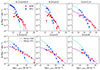 |
Fig. 1. Comparisons of RLFs of our mock AGNs (red) and SFGs (blue) to the results in Wang et al. (2024) (magenta and cyan data points respectively), separated into different redshift bins. The magenta and cyan lines are best-fit RLF models in Wang et al. (2024) for AGNs and SFGs, respectively. |
 (7)
(7)
where Vmax, i = Vzmax,i − Vzmin, i, with Vzmax, i being the co-moving volume at the maximum redshift where the i th source can be observed given the detection limit, and Vzmin, i being the co-moving volume at the lower boundary of the corresponding redshift bin. We find a good agreement between our mock radio sources and their results up to z ∼ 4 for both populations.
In Fig. 2, we compare the RLF of our mock AGNs (red dots) with several literature works. We did not apply any selection cut this time to explore the lower radio luminosity regime. McAlpine et al. (2013) selected 1054 radio sources detected at 1.4 GHz from the VIRMOS Very Large Telescope Deep Survey (VVDS, Bondi et al. 2003) covering 1 deg2, reaching a 5σ limit of 80 μJy. Padovani et al. (2015) selected 765 radio sources covering 0.285 deg2 in the Extended Chandra Deep Field-South (E-CDFS) with 1.4 GHz flux density ≥32.5 μJy. Schreiber et al. (2017) made use of the deep VLA-COSMOS data, containing more than 1800 radio AGNs spanning a wide redshift range out to z ∼ 5. We found consistent results with literature works at several redshift bins in overlapped luminosity range. On the other hand, unlike previous studies that have drawn sources based on extrapolated RLFs (e.g., Bonaldi et al. 2019), we found reduced 1.4 GHz RLF at the low-luminosity end above z = 0.4, indicating fewer less luminous radio AGNs at early epochs than simple extrapolations. This is reasonable given the fact that fewer galaxies can grow into massive galaxies with M⋆ > 1010 in the early Universe compared to in the Local Universe. In addition, SFRMS is higher toward higher redshifts, which results in larger Llimit 1.4 GHz. Therefore, the RLF cannot extrapolate to very faint regime at high redshifts. Currently there is no available observational data probing this fainter regime, more powerful next-generation facilities (e.g., SKA) may help unveil this mystery.
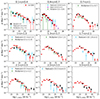 |
Fig. 2. Comparisons of RLFs of our mock AGNs (red) to literature data (McAlpine et al. 2013; Padovani et al. 2015; Schreiber et al. 2017), separated into different redshift bins. |
In Fig. 3, we compare the RLF of our mock SFGs (blue dots) to other literature data. Again, we did not apply any flux density selection criterion. Padovani et al. (2011) studied a sample of 256 1.4 GHz selected sources in the CDFS field, reaching a flux density limit of 43 μJy at the field center. A more recent work by Novak et al. (2017) took advantage of the deep VLA-COSMOS 3 GHz observations and selected ∼6000 SFGs spanning a wide redshift range out z ∼ 5 across 2 deg2. We also found an excellent agreement with real observations, even at the low-luminosity end until z ∼ 2. However, more sensitive data are needed to verify the low-luminosity end of the RLF toward higher redshifts.
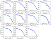 |
Fig. 3. Comparisons of RLFs of our mock SFGs (blue) to literature data (Padovani et al. 2011; McAlpine et al. 2013; Novak et al. 2017), separated into different redshift bins. |
3.2. Differential source counts
In Fig. 4, we compare the normalized source counts of our mock radio sources at 150 MHz, 1.4 GHz, and 3 GHz to various observational data and model predictions. An early study in Condon (1984) combined several 1.4 GHz surveys of three different instruments; namely, the National Radio Astronomy Observatory (NRAO) 91m telescope for sources stronger than 2 Jy, VLA, and Westerbork. Bondi et al. (2008) investigated the early release of COSMOS-VLA 1.4 GHz project with a resolution of 1.5″ and a sensitivity of ∼11 μJy, yielding ∼3600 radio sources. Vernstrom et al. (2016) studied 558 sources detected above 5σ at 3 GHz in the Lockman Hole North field, with a instrument noise of 1.01  . Smolčić et al. (2017b) took advantage of the deeper VLA-COSMOS data, providing 10830 radio sources detected above 5σ at 3 GHz, reaching a median rms of 2.3
  . More recently, Matthews et al. (2021) measured 1.4 GHz source counts based on MeerKAT DEEP2 images for flux densities below 2.5 mJy and NRAO VLA Sky Survey (NVSS) for flux densities above 2.5 mJy. van der Vlugt et al. (2021) present ultra deep VLA 3 GHz observations in the COSMOS field, reaching median rms of 0.53
  in a total area of 180 arcmin2.
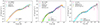 |
Fig. 4. Differential source counts of our catalog at various bands and comparisons to literature work. Left: Comparisons of differential source counts at 150 MHz to observations in Franzen et al. (2016), Mandal et al. (2021), Bondi et al. (2024) along with S3 and TRECS simulations (Wilman et al. 2008, Bonaldi et al. 2019). Middle: Comparisons of differential source counts at 1.4 GHz to observations in Condon (1984), Bondi et al. (2008), Smolčić et al. (2017b), Matthews et al. (2021), theoretical work in Bonato et al. (2017), along with S3 and TRECS simulations (Wilman et al. 2008; Bonaldi et al. 2019). Right: Comparisons of differential source counts at 3 GHz to observations in Vernstrom et al. (2016), Smolčić et al. (2017b), van der Vlugt et al. (2021), P(D) analysis in Vernstrom et al. (2014) and the TRECS simulation (Bonaldi et al. 2019). |
At low frequencies, Franzen et al. (2016) studied 154 MHz images using the Murchison Widefield Array (MWA), covering a large sky area of 570 deg2 with rms noise of 4–5 mJy beam−1. With the advent of more powerful low-frequency facility LOFAR, Mandal et al. (2021) and Bondi et al. (2024) were able to push the 154 MHz flux density limit down to a few tens of μJy beam−1, in combined ELAIS-N1, Lockman Hole, and Boötes fields as well as the Euclid Deep Field North (EDFN) field, respectively.
We found consistent results with observational data for all three frequencies. Toward lower flux densities, our source counts are more consistent with confusion amplitude distribution P(D) analysis in Vernstrom et al. (2014) at 3 GHz and theoretical models in Bonato et al. (2017) at 1.4 GHz, respectively. Here, P(D) is the probability distribution of peak flux densities in an image. A P(D) analysis can allow for a statistical estimate of source counts below the confusion limit of surveys. Vernstrom et al. (2014) fitted their P(D) models to 3 GHz observations in the Lockman Hole field and managed to constrain the source counts down to 50 nJy, which is a factor of 20 below the rms confusion. Bonato et al. (2017) derived source counts using empirical relations between SFR and free-free emission and synchrotron luminosity for SFGs, along with RLF models for AGNs from Massardi et al. (2010). This good agreement between our work and their results suggests the feasibility of using qIR of SFGs to derive radio source counts at fainter end, once the IR luminosities of SFGs are known. Still, more powerful next-generation radio facilities are needed to further investigate this faint regime.
3.3. Clustering of radio AGNs
We verified the clustering of our mock radio AGNs by calculating the angular TPCF ω(θ). As in Bonaldi et al. (2019), we adopted the Hamilton (1993) estimator:
where DD, DR, and RR are the number of galaxy pairs between the data and data samples, data and random samples, and random and random samples, respectively.
Hale et al. (2018) measured the angular TPCF of the deep 3 GHz detected sources in the COSMOS field. They classified AGNs based on a wide range of criteria such as X-ray luminosity, mid-IR color, and so on (see Smolčić et al. 2017a). They used a 5σ flux density limit of ∼13 μJy at 3 GHz and fitted the observed TPCF with a power law slope of −0.8. We select a total of 6274 radio AGNs with 3 GHz flux density above 13 μJy. We randomly placed ten time more sources across the same 4 deg2 area and count the DD, DR, and RR galaxy pairs. We repeat this procedure 200 times and use the median and 25/75 percentiles of 200 outputs as final ω(θ) values. In the right panel of Fig. 5, we plotted the results and compare to the best-fit model in Hale et al. (2018). After redistributing the EGG massive galaxies and randomly assigning radio AGNs, we observed strong TPCF amplitudes at small spacial scales for radio AGNs. However, we were not able to reproduce TPCF amplitudes toward larger spacial scales as the maximum scale radius used in Soneira & Peebles (1978) algorithm in Sect. 2.4 only reaches 3′. In addition, the final slope of TPCF is more close to −1, as we adopt the same parameters of the Soneira & Peebles (1978) algorithm as used in EGG code, which they claimed that this combination of parameters can reproduce the observed α = −1 slope of TPCF of massive galaxies. In spite of these deficiencies, our work was still able to reproduce the clustering signal of radio AGNs without needing to introduce a cosmological simulation of dark matter halos.
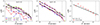 |
Fig. 5. Angular TPCF of mock galaxies and radio sources. Left: Angular TPCF of mock EGG galaxies with stellar mass > 1010 M⊙ at different redshift bins. A straight line with power law slope of −1 is also plotted. Middle: Angular TPCF of redistributed mock EGG galaxies with stellar mass > 1010 M⊙ at different redshift bins. A straight line with power law slope of −1 is also plotted. Solid and dashed lines represent active and passive galaxies respectively. Right: Angular TPCF of our mock radio AGNs with 3 GHz flux density above 13 μJy. We also plot the best-fit model from Hale et al. (2018) with a slope of −0.8. The vertical dotted line denotes the clump radius of 3′ (see Sect. 2.4). |
4. Applications of our simulation in the era of SKA and LSST
4.1. Considering the types of galaxies that can (only) be observed by SKA
In the left panel of Fig. 6, we display the 90% completeness stellar mass of galaxies that can be observed by SKA as a function of redshift. We selected SFGs with 1.4 GHz flux density above five times of 0.447 μJy beam−1, which is drawn from the SKA Sensitivity Calculator2. We assumed 5 hours observational time for a single pointing (the time spent for each VLA pointing). We expected to be able to identify many low mass galaxies at higher redshifts, ∼1010 M⊙ up to z ∼ 6, in the SKA era, significantly benefiting the study of galaxy formation in the early Universe.
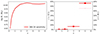 |
Fig. 6. Illustration of what improvement SKA observations will bring. Left: The 90% completeness of stellar mass of galaxies that can be observed above 5σ by SKA as a function of redshift, assuming 5 hour observation time for a single pointing. Right: Red squares denote the fraction of SKA detected galaxies that are above 27.5 mag in the SDSS-r band (approximate to LSST-r band depth) at different redshifts. At 4 < z < 6, pink cross represents the fraction of SKA detected galaxies that are above 26.1 mag in the SDSS-z band (aproximate to LSST-z band depth). |
In addition to the stellar mass range that can be observed by SKA, we would like to probe how many these SKA-detected galaxies may also be identified by large sky survey in the optical band. The LSST, currently known as the Vera C. Rubin Observatory, will carry out an ambitious survey in the optical band using its 8.4-meter primary mirror. The planned 800 exposures over ten years of observations are expected to reach a depth of r ∼ 27.5 (Ivezić et al. 2019). In the right panel of Fig. 6, we approximate the LSST-r band with the Sloan Digital Sky Survey (SDSS)-r band and we illustrate the fractions of galaxies that are fainter than 27.5 mag among those can be detected by SKA. We find an increasing fraction of SKA-detected galaxies that will be missed in deep optical surveys toward early epochs, reaching 56% at z > 4. For a sanity check, we also showed the fraction of SKA-detected sources that will be missed by longer z band observations of LSST (having a 5σ depth of 26.1 mag; Ivezić et al. 2019). There still exist a fraction of 45% of SKA detected sources that will appear invisible in the deep z band image. This plot demonstrates that SKA will play a critical role in uncovering massive dust-obscured galaxies, in complement with a deep optical survey at higher redshifts. We refer to Sect. 5.1.4 for a detailed discussion on the robustness of our simulation at z > 4.
To get a closer look of the optical morphology of SKA detected galaxies, we simulated radio images and ran source extractions. To simulate radio images we assume that radio AGNs occupy a single pixel (using pixel size of 0.24″, see Bonaldi et al. 2021) with their flux density equaling to peak flux density. On the other hand, we assumed SFGs show an exponential (Sérsic profile with n = 1) profile with their simulated flux density equaling to the total flux densities. Following Tunbridge et al. (2016), we first generated the absolute ellipticity (|E|) for SFGs through its distribution:
 (8)
(8)
with B = 0.19 and C = 0.58. Tunbridge et al. (2016) considered a two-component ellipticity, E = (E1, E2), where the first component describing elongations parallel and perpendicular to a chosen reference axis, while the second component describing elongations along the directions rotated ±45° from the reference axis. The ellipticity modulus E = |E| is connected to widely-used ellipticity e = b/a through
 (9)
(9)
The position angles are drawn from an uniform distribution between 0 and 2π. After implementing radio AGNs and SFGs, we conducted point-spread-function (PSF) convolution (using PSF size of 0.6″, see Bonaldi et al. 2021) and added Gaussian noise. As above, we ran two trials with Gaussian noise of 4.23 μJy beam−1 and 0.447 μJy beam−1 (0.6 μJy arcsec−2 and 0.06 μJy arcsec−2, respectively, assuming a beam size equaling to PSF size), which correspond to VLA and SKA observations under the same 5 hour observation per pointing, respectively. We ran pybdsf for these two mock 1.4 GHz images and present simulated JWST-F444W images with detected radio sources at four redshift bins in Fig. 7. Blue circles represent radio sources that are detected by VLA and red circles denote radio sources that will only been revealed by SKA. The unparalleled sensitivity of SKA will help us detect many more extragalactic radio sources.
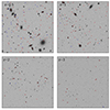 |
Fig. 7. JWST-F444W images overlaid with VLA and SKA only detected sources. Top: Simulated 2′×2′ JWST-F444W images at 0.25 < z < 0.75 and 0.75 < z < 1.25. Bottom: Simulated 4′×4′ JWST-F444W images at 1.75 < z < 2.25 and 2.75 < z < 3.25. Blue circles represent sources detected under VLA observation (with rms noise level of 4.23 μJy beam−1 at 1.4 GHz) and red circles represents sources only revealed by SKA observation (with rms noise level of 0.447 μJy beam−1) at 1.4 GHz. |
4.2. Predictions of source counts at SKA bands
In Fig. 8, we present the predicted source counts at several bands which will be observed by SKA; namely, 350 MHz, 10 GHz, and 15 GHz. As in Sect. 3, we adopt a median spectral slope of α = −0.5 for SFGs at 350 MHz and a median spectral slope of α = −0.5 for radio AGNs at all three frequencies.
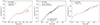 |
Fig. 8. Predicted source counts at 350 MHz, 10 GHz and 15 GHz respectively. Theoretical works from Mancuso et al. (2017) and observations from Sirothia et al. (2009), Whittam et al. (2016), Chakraborty et al. (2019), van der Vlugt et al. (2021), Jiménez-Andrade et al. (2024) are also included. |
At 350 MHz, we also included the source counts at 325 MHz and 400 MHz in the ELAIS-N1 field observed through the GMRT and the upgraded GMRT (uGMRT) by Sirothia et al. (2009) and Chakraborty et al. (2019) respectively. We corrected from 325 MHz and 400 MHz to 350 MHz, using α = −0.5 for both radio AGNs and SFGs. We found consistent results between our predictions at 350 MHz and both works.
At 10 and 15 GHz, theoretical works from Mancuso et al. (2017) and observations from Whittam et al. (2016), van der Vlugt et al. (2021), and Jiménez-Andrade et al. (2024) were also included. Whittam et al. (2016) released deep 15.7 GHz observations through the Arcminute Microkelvin Imager Large Array (AMILA) with the best rms noise of 16 μJy beam−1 in a total area of 0.56 deg2. We do not attempt to correct from 15.7 GHz to 15 GHz due to differences in spectral slopes of the two populations. Based on the model-independent approach described in Mancuso et al. (2016a,b, 2017) derived source counts at 10 GHz. van der Vlugt et al. (2021) presented ultra deep 10 GHz observations with a central rms of 0.53 μJy beam−1 in the COSMOS filed. Since their observations only cover 16 arcmin2, we randomly selected an area of the same size in our 4 deg2 simulations and calculated the source counts. We repeated this procedure 100 times to account for cosmic variance. The results are shown as blue shaded region in the right panel of Fig. 8. A more recent work by Jiménez-Andrade et al. (2024) extracted 256 radio sources in the 297 armin2 GOODS-north field. The total 380-hours observation ensured an unparalleled sensitivity of 671 nJy beam−1. At these two frequencies, we also found a good consistency between our simulations and literature works. Taken all together, our simuations are successful in reproducing observational source counts at various frequencies and can help in designing observational strategies, for example, to calculate the observation time needed to observe a sufficient number of faint objects.
4.3. Demarcation lines between radio AGNs and SFGs
In Fig. 9, we present normalized source counts at 3 GHz from radio AGNs and SFGs at various redshifts. Demarcation lines exist clearly above which radio AGNs dominate over SFGs. These demarcation lines also evolve with redshift, suggesting that there is a higher luminosity threshold for radio AGNs toward higher redshifts. This is reasonable given enhanced SFR in star forming MS galaxies in the early Universe, indicating that radio AGNs must possess higher energy to outshine their host galaxies. Other frequencies share similar features. We calculate the demarcation flux density at each band and redshift bin by simply using a powerlaw to fit three nearby data points, where the number counts from radio AGNs and SFGs intersect. We list them in Table 2. These flux densities can be utilized as selection criteria for radio AGNs at different redshifts at different bands, rather than adopting an universal luminosity cut across a wide redshift range.
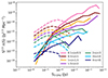 |
Fig. 9. Source counts from radio AGNs (solid lines) and SFGs (dashed lines) in different redshift bins at 3 GHz. Other frequencies show similar features. |
Demarcation flux densities for number counts from radio AGNs and SFGs at different frequencies and redshift bins.
5. Discussion
5.1. Deficiencies of our simulation
5.1.1. Lack of host halo information
Galaxies in simulations are usually accompanied by information of their host halo as dark matter halos are fundamental to their formation and can be designed through ΛCDM cosmology. For example, in the TRECS simulation, Bonaldi et al. (2019) first generated dark matter halos based on the Planck Millennium simulation (Baugh et al. 2019) and associated them to radio AGNs and SFGs based on their occurrence as a function of dark matter halo mass. However, as they are inherited from EGG, our simulations do not include host halo information and the underlying large-scale structures. Instead, we utilized a special Soneira & Peebles (1978) algorithm to add an extra clustering signal for our mock radio AGNs other than simply randomly populating in massive galaxies. Although the dark matter mass can be easily derived from stellar mass to halo mass relation (e.g., Moster et al. 2010; Behroozi et al. 2013, 2019), we cannot reproduce the clustering signal at larger scales due to the limitations of this method, let alone large-scale structures such as filaments. Nonetheless, this lack of large-scale clustering will not affect the main focus of our simulations and is beyond the scope of this paper.
5.1.2. Considering whether low mass galaxies host low luminosity radio AGNs
We assumed that radio AGNs residing in host galaxies are characterized by a stellar mass above 1010 M⊙ (see Sect. 2.2). This is consistent with literature work that found radio AGNs are mainly hosted by massive galaxies. For example, Best et al. (2005) selected 2215 radio-loud AGNs at 0.03 < z < 0.3 and found that the fraction of galaxies below 1010 M⊙ hosting radio-loud AGNs with L1.4 GHz > 1023 W Hz−1 is nearly zero. Nonetheless, we cannot rule out the possibility of low-mass galaxies hosting less powerful radio AGNs. We can easily circumvent this issue by simply extrapolating the radio AGN probabilities in Formula (2) to lower stellar mass regime. However, it will produce much more radio AGNs since galaxies below 1010 M⊙ are way more than galaxies above 1010 M⊙: nearly 60% of EGG galaxies have stellar mass between 108 − 1010 M⊙, while only ∼4% of EGG galaxies are above 1010 M⊙, under magnitude cut of F444W = 28 mag. This simple extrapolation will lead to an inconsistency in terms of the radio AGN number density, especially at low redshifts. At higher redshifts, this problem is relieved as these low-mass galaxies are hardly observable, given the nominal 3 GHz flux limit of 2.3 μJy beam−1. To maintain consistency, we still retained the 1010 M⊙ threshold when assign radio AGNs across all redshifts. Whether (and how many) low-mass galaxies host (low-luminosity and potentially high-luminosity) radio AGNs are an open question for future observational surveys. Hopefully the upcoming deeper SKA observations will help to answer this question. On the other hand, the question of whether the 1010 M⊙ threshold is less massive for radio AGNs at higher redshifts is still wide open. However, investigating the boundary stellar mass is beyond the scope of this work. In this work we stick to the 1010 M⊙ threshold when assigning radio AGNs. Furthermore, even though these 1010 M⊙ galaxies are assigned to host radio AGNs, it becomes harder to observe them toward earlier epochs. It is only with SKA that these radio-AGN-hosting galaxies with stellar mass around 1010 M⊙ could feasibly be detected, as indicated in Fig. 6. We leave this question for a future work.
5.1.3. The lack of extended radio sources
Our studies are based on radio observations from COSMOS-VLA survey, which is characterized by a supreme resolution of 0 75 (Smolčić et al. 2017b). However, interferometric observations are known to bias against extended radio sources, such as sources with elongated radio lobes (FRI and FRII radio-loud galaxies). We have not attempted to fix this issue by adding extra FRI and FRII sources due to lack of extensive studies on their fractions as a function of stellar mass and redshift. We caution on the use of our simulations in the context of the nearby Universe. This lack of extended sources may explain partly the lack of extreme source of number counts in Fig. 4. We hope more extensive data in the future (e.g., SKA observations) would help to bridge this gap.
5.1.4. Mock galaxy and radio AGNs at z > 4
The mock galaxy catalog generated by EGG is built upon empirical knowledge on galaxy evolution across cosmic history. So far, our understanding toward the high-redshift Universe is still largely incomplete due to limited data coverage. To generate mock passive galaxies at z > 4, the EGG code adopts the same parameters of their stellar mass functions at low redshifts, with the assumption of a fraction of 15% given the difficulty to fit individual stellar mass functions with small sample size. When we assign radio AGNs based on AGN probability, we need to extrapolate the redshift-dependent Equations (2) and (5) to 4 < z < 6, as Wang et al. (2024) only investigated radio AGN probability at z < 4 due to limited sample size at higher redshifts. For SFGs, the parent sample used in Delvecchio et al. (2021) is restricted to z < 4.5, so we extrapolate their redshift- and mass- dependent qIR to obtain 1.4 GHz radio luminosity for non-AGNs at z > 4.5. Despite these simple extrapolations, our mock radio catalogs have succeeded in recovering RLFs of both radio AGNs and SFGs at z > 4, suggesting the universality of these scaling relationships across a wide redshift range and the feasibility of our method in reproducing the ERB. Upcoming advanced data from new facilities, for example, a more precise constraint of stellar mass functions for passive galaxies at z > 4 with new JWST observations, would be of great help to the robustness of our mock catalog at high redshifts.
5.2. Coution on the contribution to the ERB from radio AGN and SFGs
In Fig. 10, we plot the total flux densities per steradian of both radio AGNs and SFGs along with their sum at various bands. At first glance, the contribution from SFGs and radio AGNs at frequencies higher than 3 GHz are broadly consistent with model predictions in Massardi et al. (2010) and observations, while showing significantly lower contribution from radio AGNs toward lower frequencies. Compared to TRECS simulation, we find that this large discrepancy at 150 MHz is mainly attributed to four extremely bright radio AGNs, with  at 0.4 < z < 0.7 existing in TRECS simulation (although they are lacking in our simulation). Therefore, we conducted out a test by injecting one radio AGN with
  at z = 0.4 per square degree. The added contributions from radio AGNs are shown as red stars. The significant elevation by merely one source per square degree indicates the caution in comparing radio AGN and SFG contribution, especially at low frequencies. Adding one bright AGN will not change their RLF significantly (in fact, the radio AGN LF at 0.4 < z < 0.7 derived from TRECS simulation is in broad agreement with but slightly higher at the brightest end than observations in Kondapally et al. 2022), but their contribution to the ERB will be substantially boosted. The driving factors causing one more or fewer bright radio AGNs may be attributed to a biased sample against extended FRII sources (which can reach
  at z ∼ 0.4, e.g., de Jong et al. 2024) in Wang et al. (2024), leading to a smaller fraction of radio-bright AGNs calculated via Formula (2). We ran a sanity check by assigning radio AGNs 200 times and display the 5/95 percentile distribution of their contribution as shaded pink region. The contribution from radio AGNs is loosely constrained, with the majority of them merely differing approximately in one bright source per square degree, while the RLF (as well as source counts) remain in good agreement with observations. Thus, we urge caution when using radio AGN contribution to the ERB, either in theoretical or observational analyses.
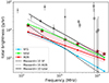 |
Fig. 10. Contribution from radio AGNs (red) and SFGs (blue) along with their sum (green) to the ERB at various frequencies. We also compare our results with the model from Massardi et al. (2010). Data points are from Bridle (1967), Wall et al. (1970), Fixsen (2009) (see Figure 9 in Massardi et al. 2010). The red stars denote the contribution from radio AGN plus a single source with |
6. Summary
Radio observations play a critical role in helping us understand how galaxies assemble and evolve across the history of our Universe. Realistic simulations of extragalactic radio background are important in designing radio surveys and developing radio facilities. The current simulations are primarily built on the well-studied RLFs of different populations and, despite their success in recovering the ERB, it is difficult to gain insights into other physical information of radio sources; in addition, they leave the physical origins behind the scenario overlooked. We utilized a novel method to associate radio properties with the rich physical information of galaxies such stellar mass, SFRs, and multiwavelength flux densities, benefiting the study of galaxy evolution in a synergistic way.
Based on mock multi-wavelength source catalog generated by EGG code, we assigned radio AGNs according to well-defined radio AGN probabilities as a function of radio luminosity, stellar mass, and redshift. We assumed that radio AGNs only populating in massive galaxies with stellar masses above 1010 M⊙ and we made use of the star forming main sequence to determine the luminosity threshold above which radio AGN dominates. For SFGs, we took advantage of the tight correlation between IR luminosity and radio luminosity to derive their radio luminosities. Through this method, we have managed to link radio flux densities to a plethora of physical information embedded in a mock galaxy catalog.
We successfully recovered a number of observables, including 1.4 GHz RLFs of both radio AGNs and SFGs, as well as source counts at various frequencies. These results suggest these two populations are important building blocks making up the ERB. Our successful simulation can help designing observational strategy of radio surveys and evaluating the performance of future radio facilities. The link between radio properties and abundant physical properties will benefit studies of galaxy evolution in a synergistic way, allowing us to explore the multiwavelength counterparts of radio sources. We found that a significant fraction of 45–56% radio sources at z > 4 that may feasibly be detected by SKA, the next generation of radio facilities, will appear invisible in the future deepest optical survey carried out by LSST. This demonstrates the unparalleled role that deep radio observations play in finding faint dust-obscured galaxies in the early Universe. Along with this work, we have publicly released our mock sources.
Data availability
Our mock catalog can be accessed via Zenodo3 or Google Drive4. The columns are listed in Table A.1.
https://sensitivity-calculator.skao.int/mid. We adopt default AA4 configuration at Band 2, centered at 1.4 GHz with a bandwidth of 500 MHz under natural weighting.
Acknowledgments
We thank the anonymous referee for a through and constructive report. This work was supported by National Natural Science Foundation of China (Project No. 12173017 and Key Project No. 12141301), National Key R&D Program of China (2023YFA1605600) and the China Manned Space Project (No. CMS-CSST-2021-A07). F.Y.G acknowledges supports by Jiangsu Provincial Outstanding Postdoctoral Program ([2023]209) and Yuxiu Young Scholars Program in Nanjing University. Y.J.W. acknowledges supports by National Natural Science Foundation of China (Project No. 12403019) and the National Science Foundation of Jiangsu Province (BK20241188).
References
- Alberts, S., Rujopakarn, W., Rieke, G. H., Jagannathan, P., & Nyland, K. 2020, ApJ, 901, 168 [NASA ADS] [CrossRef] [Google Scholar]
- An, F., Vaccari, M., Best, P. N., et al. 2024, MNRAS, 528, 5346 [NASA ADS] [CrossRef] [Google Scholar]
- Baugh, C. M., Gonzalez-Perez, V., Lagos, C. D. P., et al. 2019, MNRAS, 483, 4922 [NASA ADS] [CrossRef] [Google Scholar]
- Behroozi, P. S., Wechsler, R. H., & Conroy, C. 2013, ApJ, 770, 57 [NASA ADS] [CrossRef] [Google Scholar]
- Behroozi, P., Wechsler, R. H., Hearin, A. P., & Conroy, C. 2019, MNRAS, 488, 3143 [NASA ADS] [CrossRef] [Google Scholar]
- Bell, E. F. 2003, ApJ, 586, 794 [Google Scholar]
- Best, P. N., Kauffmann, G., Heckman, T. M., et al. 2005, MNRAS, 362, 25 [Google Scholar]
- Béthermin, M., Wu, H.-Y., Lagache, G., et al. 2017, A&A, 607, A89 [Google Scholar]
- Bonaldi, A., Bonato, M., Galluzzi, V., et al. 2019, MNRAS, 482, 2 [Google Scholar]
- Bonaldi, A., An, T., Brüggen, M., et al. 2021, MNRAS, 500, 3821 [Google Scholar]
- Bonato, M., Negrello, M., Mancuso, C., et al. 2017, MNRAS, 469, 1912 [Google Scholar]
- Bondi, M., Ciliegi, P., Zamorani, G., et al. 2003, A&A, 403, 857 [NASA ADS] [CrossRef] [EDP Sciences] [Google Scholar]
- Bondi, M., Ciliegi, P., Schinnerer, E., et al. 2008, ApJ, 681, 1129 [Google Scholar]
- Bondi, M., Scaramella, R., Zamorani, G., et al. 2024, A&A, 683, A179 [NASA ADS] [CrossRef] [EDP Sciences] [Google Scholar]
- Bridle, A. H. 1967, MNRAS, 136, 219 [NASA ADS] [Google Scholar]
- Brown, M. J. I., Moustakas, J., Kennicutt, R. C., et al. 2017, ApJ, 847, 136 [Google Scholar]
- Chakraborty, A., Roy, N., Datta, A., et al. 2019, MNRAS, 490, 243 [Google Scholar]
- Condon, J. J. 1984, ApJ, 284, 44 [NASA ADS] [CrossRef] [Google Scholar]
- Conroy, C. 2013, ARA&A, 51, 393 [NASA ADS] [CrossRef] [Google Scholar]
- Croton, D. J., Springel, V., White, S. D. M., et al. 2006, MNRAS, 365, 11 [Google Scholar]
- Daddi, E., Dickinson, M., Morrison, G., et al. 2007, ApJ, 670, 156 [NASA ADS] [CrossRef] [Google Scholar]
- Dale, D. A., & Helou, G. 2002, ApJ, 576, 159 [Google Scholar]
- Davidzon, I., Ilbert, O., Laigle, C., et al. 2017, A&A, 605, A70 [NASA ADS] [CrossRef] [EDP Sciences] [Google Scholar]
- Davies, L. J. M., Huynh, M. T., Hopkins, A. M., et al. 2017, MNRAS, 466, 2312 [Google Scholar]
- de Jong, J. M. G. H. J., Röttgering, H. J. A., Kondapally, R., et al. 2024, A&A, 683, A23 [NASA ADS] [CrossRef] [EDP Sciences] [Google Scholar]
- Delvecchio, I., Daddi, E., Sargent, M. T., et al. 2021, A&A, 647, A123 [NASA ADS] [CrossRef] [EDP Sciences] [Google Scholar]
- Duncan, K., Conselice, C. J., Mortlock, A., et al. 2014, MNRAS, 444, 2960 [Google Scholar]
- Fixsen, D. J. 2009, ApJ, 707, 916 [Google Scholar]
- Franzen, T. M. O., Jackson, C. A., Offringa, A. R., et al. 2016, MNRAS, 459, 3314 [NASA ADS] [CrossRef] [Google Scholar]
- Garn, T., Green, D. A., Riley, J. M., & Alexander, P. 2009, MNRAS, 397, 1101 [Google Scholar]
- Guo, Y., Ferguson, H. C., Giavalisco, M., et al. 2013, ApJS, 207, 24 [NASA ADS] [CrossRef] [Google Scholar]
- Hale, C. L., Jarvis, M. J., Delvecchio, I., et al. 2018, MNRAS, 474, 4133 [NASA ADS] [CrossRef] [Google Scholar]
- Hamilton, A. J. S. 1993, ApJ, 417, 19 [Google Scholar]
- Hartley, W. G., Lane, K. P., Almaini, O., et al. 2008, MNRAS, 391, 1301 [NASA ADS] [CrossRef] [Google Scholar]
- Hartley, W. G., Almaini, O., Cirasuolo, M., et al. 2010, MNRAS, 407, 1212 [NASA ADS] [CrossRef] [Google Scholar]
- Hinshaw, G., Larson, D., Komatsu, E., et al. 2013, ApJS, 208, 19 [Google Scholar]
- Ivezić, Ž., Kahn, S. M., Tyson, J. A., et al. 2019, ApJ, 873, 111 [Google Scholar]
- Jiang, L., Fan, X., Ivezić, Ž., et al. 2007, ApJ, 656, 680 [Google Scholar]
- Jiménez-Andrade, E. F., Murphy, E. J., Momjian, E., et al. 2024, ApJ, 972, 89 [CrossRef] [Google Scholar]
- Jin, S., Daddi, E., Liu, D., et al. 2018, ApJ, 864, 56 [Google Scholar]
- Kellermann, K. I., Sramek, R., Schmidt, M., Shaffer, D. B., & Green, R. 1989, AJ, 98, 1195 [Google Scholar]
- Kondapally, R., Best, P. N., Cochrane, R. K., et al. 2022, MNRAS, 513, 3742 [NASA ADS] [CrossRef] [Google Scholar]
- Magdis, G. E., Daddi, E., Béthermin, M., et al. 2012, ApJ, 760, 6 [NASA ADS] [CrossRef] [Google Scholar]
- Magliocchetti, M., Popesso, P., Brusa, M., et al. 2017, MNRAS, 464, 3271 [NASA ADS] [CrossRef] [Google Scholar]
- Mancuso, C., Lapi, A., Shi, J., et al. 2016a, ApJ, 833, 152 [NASA ADS] [CrossRef] [Google Scholar]
- Mancuso, C., Lapi, A., Shi, J., et al. 2016b, ApJ, 823, 128 [NASA ADS] [CrossRef] [Google Scholar]
- Mancuso, C., Lapi, A., Prandoni, I., et al. 2017, ApJ, 842, 95 [Google Scholar]
- Mandal, S., Prandoni, I., Hardcastle, M. J., et al. 2021, A&A, 648, A5 [EDP Sciences] [Google Scholar]
- Massardi, M., Bonaldi, A., Negrello, M., et al. 2010, MNRAS, 404, 532 [NASA ADS] [Google Scholar]
- Matthews, A. M., Condon, J. J., Cotton, W. D., & Mauch, T. 2021, ApJ, 909, 193 [NASA ADS] [CrossRef] [Google Scholar]
- McAlpine, K., Jarvis, M. J., & Bonfield, D. G. 2013, MNRAS, 436, 1084 [CrossRef] [Google Scholar]
- Moster, B. P., Somerville, R. S., Maulbetsch, C., et al. 2010, ApJ, 710, 903 [Google Scholar]
- Murphy, E. J., Momjian, E., Condon, J. J., et al. 2017, ApJ, 839, 35 [Google Scholar]
- Muzzin, A., Marchesini, D., Stefanon, M., et al. 2013, ApJ, 777, 18 [NASA ADS] [CrossRef] [Google Scholar]
- Noeske, K. G., Weiner, B. J., Faber, S. M., et al. 2007, ApJ, 660, L43 [CrossRef] [Google Scholar]
- Novak, M., Smolčić, V., Delhaize, J., et al. 2017, A&A, 602, A5 [NASA ADS] [CrossRef] [EDP Sciences] [Google Scholar]
- Padovani, P., Miller, N., Kellermann, K. I., et al. 2011, ApJ, 740, 20 [Google Scholar]
- Padovani, P., Bonzini, M., Kellermann, K. I., et al. 2015, MNRAS, 452, 1263 [Google Scholar]
- Pearson, W. J., Wang, L., Hurley, P. D., et al. 2018, A&A, 615, A146 [NASA ADS] [CrossRef] [EDP Sciences] [Google Scholar]
- Rodighiero, G., Daddi, E., Baronchelli, I., et al. 2011, ApJ, 739, L40 [Google Scholar]
- Salpeter, E. E. 1955, ApJ, 121, 161 [Google Scholar]
- Santini, P., Fontana, A., Castellano, M., et al. 2017, ApJ, 847, 76 [NASA ADS] [CrossRef] [Google Scholar]
- Schmidt, M., & Green, R. F. 1983, ApJ, 269, 352 [NASA ADS] [CrossRef] [Google Scholar]
- Schreiber, C., Pannella, M., Elbaz, D., et al. 2015, A&A, 575, A74 [NASA ADS] [CrossRef] [EDP Sciences] [Google Scholar]
- Schreiber, C., Elbaz, D., Pannella, M., et al. 2017, A&A, 602, A96 [NASA ADS] [CrossRef] [EDP Sciences] [Google Scholar]
- Sirothia, S. K., Dennefeld, M., Saikia, D. J., et al. 2009, MNRAS, 395, 269 [Google Scholar]
- Smolčić, V., Delvecchio, I., Zamorani, G., et al. 2017a, A&A, 602, A2 [NASA ADS] [CrossRef] [EDP Sciences] [Google Scholar]
- Smolčić, V., Novak, M., Bondi, M., et al. 2017b, A&A, 602, A1 [Google Scholar]
- Smolčić, V., Novak, M., Delvecchio, I., et al. 2017c, A&A, 602, A6 [NASA ADS] [CrossRef] [EDP Sciences] [Google Scholar]
- Soneira, R. M., & Peebles, P. J. E. 1978, AJ, 83, 845 [NASA ADS] [CrossRef] [Google Scholar]
- Speagle, J. S., Steinhardt, C. L., Capak, P. L., & Silverman, J. D. 2014, ApJS, 214, 15 [Google Scholar]
- Tadhunter, C. 2016, A&A Rev., 24, 10 [NASA ADS] [CrossRef] [Google Scholar]
- Tomczak, A. R., Quadri, R. F., Tran, K.-V. H., et al. 2014, ApJ, 783, 85 [Google Scholar]
- Tunbridge, B., Harrison, I., & Brown, M. L. 2016, MNRAS, 463, 3339 [NASA ADS] [CrossRef] [Google Scholar]
- van der Vlugt, D., Algera, H. S. B., Hodge, J. A., et al. 2021, ApJ, 907, 5 [NASA ADS] [CrossRef] [Google Scholar]
- van der Wel, A., Franx, M., van Dokkum, P. G., et al. 2014, ApJ, 788, 28 [Google Scholar]
- Vernstrom, T., Scott, D., Wall, J. V., et al. 2014, MNRAS, 440, 2791 [CrossRef] [Google Scholar]
- Vernstrom, T., Scott, D., Wall, J. V., et al. 2016, MNRAS, 462, 2934 [Google Scholar]
- Wall, J. V., Chu, T. Y., & Yen, J. L. 1970, Aust. J. Phys., 23, 45 [NASA ADS] [Google Scholar]
- Wang, L., Gao, F., Duncan, K. J., et al. 2019, A&A, 631, A109 [NASA ADS] [CrossRef] [EDP Sciences] [Google Scholar]
- Wang, Y., Wang, T., Liu, D., et al. 2024, A&A, 685, A79 [NASA ADS] [CrossRef] [EDP Sciences] [Google Scholar]
- Weaver, J. R., Kauffmann, O. B., Ilbert, O., et al. 2022, ApJS, 258, 11 [NASA ADS] [CrossRef] [Google Scholar]
- Whitaker, K. E., Labbé, I., van Dokkum, P. G., et al. 2011, ApJ, 735, 86 [Google Scholar]
- Whitaker, K. E., van Dokkum, P. G., Brammer, G., & Franx, M. 2012, ApJ, 754, L29 [Google Scholar]
- Whittam, I. H., Riley, J. M., Green, D. A., et al. 2016, MNRAS, 457, 1496 [NASA ADS] [CrossRef] [Google Scholar]
- Wilman, R. J., Miller, L., Jarvis, M. J., et al. 2008, MNRAS, 388, 1335 [NASA ADS] [Google Scholar]
- Yun, M. S., Reddy, N. A., & Condon, J. J. 2001, ApJ, 554, 803 [Google Scholar]
Appendix A: Summary of our mock catalog
We release our mock catalog with their columns listed in Table A.1.
Structure of our 4 deg2 mock galaxy catalog.
All Tables
Demarcation flux densities for number counts from radio AGNs and SFGs at different frequencies and redshift bins.
All Figures
|
Fig. 1. Comparisons of RLFs of our mock AGNs (red) and SFGs (blue) to the results in Wang et al. (2024) (magenta and cyan data points respectively), separated into different redshift bins. The magenta and cyan lines are best-fit RLF models in Wang et al. (2024) for AGNs and SFGs, respectively. |
| In the text | |
|
Fig. 2. Comparisons of RLFs of our mock AGNs (red) to literature data (McAlpine et al. 2013; Padovani et al. 2015; Schreiber et al. 2017), separated into different redshift bins. |
| In the text | |
|
Fig. 3. Comparisons of RLFs of our mock SFGs (blue) to literature data (Padovani et al. 2011; McAlpine et al. 2013; Novak et al. 2017), separated into different redshift bins. |
| In the text | |
|
Fig. 4. Differential source counts of our catalog at various bands and comparisons to literature work. Left: Comparisons of differential source counts at 150 MHz to observations in Franzen et al. (2016), Mandal et al. (2021), Bondi et al. (2024) along with S3 and TRECS simulations (Wilman et al. 2008, Bonaldi et al. 2019). Middle: Comparisons of differential source counts at 1.4 GHz to observations in Condon (1984), Bondi et al. (2008), Smolčić et al. (2017b), Matthews et al. (2021), theoretical work in Bonato et al. (2017), along with S3 and TRECS simulations (Wilman et al. 2008; Bonaldi et al. 2019). Right: Comparisons of differential source counts at 3 GHz to observations in Vernstrom et al. (2016), Smolčić et al. (2017b), van der Vlugt et al. (2021), P(D) analysis in Vernstrom et al. (2014) and the TRECS simulation (Bonaldi et al. 2019). |
| In the text | |
|
Fig. 5. Angular TPCF of mock galaxies and radio sources. Left: Angular TPCF of mock EGG galaxies with stellar mass > 1010 M⊙ at different redshift bins. A straight line with power law slope of −1 is also plotted. Middle: Angular TPCF of redistributed mock EGG galaxies with stellar mass > 1010 M⊙ at different redshift bins. A straight line with power law slope of −1 is also plotted. Solid and dashed lines represent active and passive galaxies respectively. Right: Angular TPCF of our mock radio AGNs with 3 GHz flux density above 13 μJy. We also plot the best-fit model from Hale et al. (2018) with a slope of −0.8. The vertical dotted line denotes the clump radius of 3′ (see Sect. 2.4). |
| In the text | |
|
Fig. 6. Illustration of what improvement SKA observations will bring. Left: The 90% completeness of stellar mass of galaxies that can be observed above 5σ by SKA as a function of redshift, assuming 5 hour observation time for a single pointing. Right: Red squares denote the fraction of SKA detected galaxies that are above 27.5 mag in the SDSS-r band (approximate to LSST-r band depth) at different redshifts. At 4 < z < 6, pink cross represents the fraction of SKA detected galaxies that are above 26.1 mag in the SDSS-z band (aproximate to LSST-z band depth). |
| In the text | |
|
Fig. 7. JWST-F444W images overlaid with VLA and SKA only detected sources. Top: Simulated 2′×2′ JWST-F444W images at 0.25 < z < 0.75 and 0.75 < z < 1.25. Bottom: Simulated 4′×4′ JWST-F444W images at 1.75 < z < 2.25 and 2.75 < z < 3.25. Blue circles represent sources detected under VLA observation (with rms noise level of 4.23 μJy beam−1 at 1.4 GHz) and red circles represents sources only revealed by SKA observation (with rms noise level of 0.447 μJy beam−1) at 1.4 GHz. |
| In the text | |
|
Fig. 8. Predicted source counts at 350 MHz, 10 GHz and 15 GHz respectively. Theoretical works from Mancuso et al. (2017) and observations from Sirothia et al. (2009), Whittam et al. (2016), Chakraborty et al. (2019), van der Vlugt et al. (2021), Jiménez-Andrade et al. (2024) are also included. |
| In the text | |
|
Fig. 9. Source counts from radio AGNs (solid lines) and SFGs (dashed lines) in different redshift bins at 3 GHz. Other frequencies show similar features. |
| In the text | |
|
Fig. 10. Contribution from radio AGNs (red) and SFGs (blue) along with their sum (green) to the ERB at various frequencies. We also compare our results with the model from Massardi et al. (2010). Data points are from Bridle (1967), Wall et al. (1970), Fixsen (2009) (see Figure 9 in Massardi et al. 2010). The red stars denote the contribution from radio AGN plus a single source with |
| In the text | |
Current usage metrics show cumulative count of Article Views (full-text article views including HTML views, PDF and ePub downloads, according to the available data) and Abstracts Views on Vision4Press platform.
Data correspond to usage on the plateform after 2015. The current usage metrics is available 48-96 hours after online publication and is updated daily on week days.
Initial download of the metrics may take a while.