| Issue |
A&A
Volume 660, April 2022
|
|
|---|---|---|
| Article Number | A111 | |
| Number of page(s) | 21 | |
| Section | Cosmology (including clusters of galaxies) | |
| DOI | https://doi.org/10.1051/0004-6361/202142664 | |
| Published online | 22 April 2022 | |
Moment expansion of polarized dust SED: A new path towards capturing the CMB B-modes with LiteBIRD
1
IRAP, Université de Toulouse, CNRS, CNES, UPS, Toulouse, France
e-mail: leo.vacher@irap.omp.eu
2
Department of Physics, University of Oxford, Denys Wilkinson Building, Keble Road, Oxford OX1 3RH, UK
3
Kavli Institute for the Physics and Mathematics of the Universe (Kavli IPMU, WPI), UTIAS, The University of Tokyo, Kashiwa, Chiba 277-8583, Japan
4
Laboratoire de Physique de l’Ecole normale supérieure, ENS, Université PSL, CNRS, Sorbonne Université, Université Paris-Diderot, Sorbonne Paris Cité, Paris, France
5
Instituto de Fisica de Cantabria (CSIC-Universidad de Cantabria), Avda. de los Castros s/n, 39005 Santander, Spain
6
Jodrell Bank Centre for Astrophysics, Department of Physics and Astronomy, The University of Manchester, Manchester M13 9PL, UK
Received:
15
November
2021
Accepted:
18
January
2022
Accurate characterization of the polarized dust emission from our Galaxy will be decisive in the quest for the cosmic microwave background (CMB) primordial B-modes. An incomplete modeling of its potentially complex spectral properties could lead to biases in the CMB polarization analyses and to a spurious measurement of the tensor-to-scalar ratio r. It is particularly crucial for future surveys like the LiteBIRD satellite, the goal of which is to constrain the faint primordial signal leftover by inflation with an accuracy on the tensor-to-scalar ratio r of the order of 10−3. Variations of the dust properties along and between lines of sight lead to unavoidable distortions of the spectral energy distribution (SED) that cannot be easily anticipated by standard component-separation methods. This issue can be tackled using a moment expansion of the dust SED, an innovative parametrization method imposing minimal assumptions on the sky complexity. In the present paper, we apply this formalism to the B-mode cross-angular power spectra computed from simulated LiteBIRD polarization data at frequencies between 100 and 402 GHz that contain CMB, dust, and instrumental noise. The spatial variation of the dust spectral parameters (spectral index β and temperature T) in our simulations lead to significant biases on r (∼21 σr) if not properly taken into account. Performing the moment expansion in β, as in previous studies, reduces the bias but does not lead to sufficiently reliable estimates of r. We introduce, for the first time, the expansion of the cross-angular power spectra SED in both β and T, showing that, at the sensitivity of LiteBIRD, the SED complexity due to temperature variations needs to be taken into account in order to prevent analysis biases on r. Thanks to this expansion, and despite the existing correlations between some of the dust moments and the CMB signal responsible for a rise in the error on r, we can measure an unbiased value of the tensor-to-scalar ratio with a dispersion as low as σr = 8.8 × 10⁻⁴.
Key words: cosmic background radiation / inflation / cosmology: observations / dust / extinction
© L. Vacher et al. 2022
 Open Access article, published by EDP Sciences, under the terms of the Creative Commons Attribution License (https://creativecommons.org/licenses/by/4.0), which permits unrestricted use, distribution, and reproduction in any medium, provided the original work is properly cited.
1. Introduction
Our present understanding of the primordial Universe relies on the paradigm of inflation (Brout et al. 1978; Starobinsky 1980; Guth 1981), introducing a phase of accelerated expansion in the first fractions of a second after the primordial singularity. Such a phenomenon is expected to leave a background of gravitational waves propagating in the primordial plasma during recombination, leaving a permanent mark imprinted in the polarization anisotropies of the cosmic microwave background (CMB): the primordial B-modes (Polnarev 1985; Kamionkowski et al. 1997; Seljak & Zaldarriaga 1997). The amplitude of the angular power spectrum of those primordial B-modes is characterized by the tensor-to-scalar ratio r, which is proportional to the energy scale at which inflation occurred (Lyth 1997). Hence, looking for this smoking gun of inflation allows us to test our best theories of fundamental physics in the primordial Universe at energy scales far beyond the reach of particle accelerators. In this scope, it is one of the biggest challenges of cosmology set out for the next decades. The best experimental upper limit on the r parameter so far is r < 0.032 (95% C.L., Tristram et al. 2021; Bicep/Keck Collaboration 2021; BICEP2/Keck & Planck Collaboration 2015).
The JAXA Lite (Light) satellite, used for the B-mode polarization and Inflation from cosmic background Radiation Detection (LiteBIRD) mission, is designed to observe the sky at large angular scales in order to constrain this parameter r down to δr = 10−3, including all sources of uncertainty (Hazumi 2018; LiteBIRD Collaboration 2020). Exploring this region of the parameter space is critical, because this order of magnitude for the tensor-to-scalar ratio is predicted by numerous physically motivated inflation models (for a review see e.g., Martin et al. 2014)
However, the success of this mission relies on our ability to treat polarized foreground signals. Indeed various diffuse astrophysical sources emit polarized B-mode signals above the primordial ones, the strongest being due to the diffuse polarized emission of our own Galaxy (Planck Collaboration IV 2020). Even in a diffuse region like the BICEP/Keck field, the Galactic B-modes are at least ten times stronger at 150 GHz than the r = 0.01 tensor B-modes targeted by the current CMB experiments (BICEP2 Collaboration & Keck Array Collaboration 2018).
The true complexity of polarized foreground emission that the next generation of CMB experiments will face is still mostly unknown today. Underestimation of this complexity can lead to the estimation of a spurious nonzero value of r (see e.g., Planck Collaboration Int. L 2017; Remazeilles et al. 2016).
At high frequencies (> 100 GHz), the thermal emission of interstellar dust grains is the main source of Galactic foreground contaminating the CMB (Krachmalnicoff et al. 2016; Planck Collaboration XI 2020). The canonical model of the spectral energy distribution (SED) of this thermal emission for intensity and polarization is given by the modified black body (MBB) law (Desert et al. 1990). This model provides a good fit to the dust polarization SED at the sensitivity of the Planck satellite (Planck Collaboration XI 2020) but it may not fully account for it at the sensitivity of future experiments (Hensley & Bull 2018). Furthermore, due to changes of physical conditions across the galaxy, spatial variations of the SEDs are present between and along the lines of sight. The former leads to what is known as frequency decorrelation in the CMB community (see e.g. Tassis & Pavlidou 2015; Planck Collaboration Int. L 2017; Pelgrims et al. 2021). Moreover, both effects lead to averaging MBBs when observing the sky (unavoidable line-of-sight or beam-integration effects). Because of the nonlinearity of the MBB law, those averaging effects will distort the SED, leading to deviations from this canonical model (Chluba et al. 2017).
Chluba et al. (2017) proposed a general framework called “moment expansion” of the SED to take into account those distortions, using a Taylor expansion around the MBB with respect to its spectral parameters (Taylor expansion of foreground SEDs was discussed in previous studies; see e.g., Stolyarov et al. 2005). This method is agnostic: it does not require any assumption on the real complexity of the polarized dust emission. The moment expansion approach thus provides a promising tool with which to model the unanticipatable complexity of the dust emission in real data.
Mangilli et al. (2021) generalized this formalism for the sake of CMB data analysis in harmonic space and for cross-angular power spectra and applied it successfully to complex simulations and Planck High-Frequency Instrument (HFI) intensity data. This latter work shows that the real complexity of Galactic foregrounds could be higher than expected, encouraging us to follow the path opened by the moment expansion formalism.
In the present work, we apply the moment expansion in harmonic space to characterize and treat the dust foreground polarized emission of LiteBIRD high-frequency simulations, using dust-emission models of increasing complexity. We discuss the ability of this method to recover an unbiased value for the r parameter, with enough accuracy to achievethe scientific objectives of the LiteBIRD mission.
In Sect. 2, we first review the formalism of moment expansion in map and harmonic domains. We then describe in Sect. 3 how we realize several sets of simulations of the sky as seen by the LiteBIRD instrument with varying dust complexity and how we estimate the angular power spectra. In Sect. 4, we describe how we estimate the moment parameters and the tensor-to-scalar ratio r in those simulations. The results are then presented in Sect. 5. Finally, we discuss those results and the future work that has to be done in the direction opened by moment expansion in Sect. 6.
2. Formalism
2.1. Characterizing the dust SED in real space
2.1.1. Modified black body model
The canonical way to characterize astrophysical dust-grain emission in every volume element of the Galaxy is given by the modified black body (MBB) function, consisting of multiplying a standard black body SED Bν(T) at a given temperature T0 by a power-law of the frequency ν with a spectral index β0. The dust intensity map ID(ν,n) observed at a frequency ν in every direction with respect to the unit vector n, can then be written as:
where A(n) is the dust intensity template at a reference frequency ν01. We know that the physical conditions (thermodynamic and dust grain properties) change through the interstellar medium across the Galaxy, depending, in an intricate fashion, on the gas velocity and density, the interstellar radiation field, the distance to the Galactic center (see e.g., Paradis et al. 2009; Ysard et al. 2015; Planck Collaboration XI 2014; Planck Collaboration IV 2020; Hutton et al. 2015; Fanciullo et al. 2015). This change of physical conditions leads to variations in β and T depending on the direction of observation n:
The SED amplitude and parameters (temperature and spectral index) are then different for every line of sight. It is therefore clear that, in order to provide a realistic model of the dust emission, the frequency and spatial dependencies may not be trivially separated.
2.1.2. Limits of the modified black body
The dust SED model given by the MBB has proven to be highly accurate (Planck Collaboration Int. XVII 2014; Planck Collaboration Int. XXII 2015). However, it must be kept in mind that this model is empirical and is therefore not expected to give a perfect description of the dust SED in the general case. Indeed, physically motivated dust grain emission models predict deviations from it (e.g., Draine & Hensley 2013). Surveys tend to show that the dust-emission properties vary across the observed 2D sky and the 3D Galaxy (Planck Collaboration XI 2020). Furthermore, in true experimental conditions, one can never directly access the pure SED of a single volume element with specific emission properties and unique spectral parameters. Averages are therefore made over different SEDs emitted from distinct regions with different physical emission properties, in a way that may not be avoided: along the line of sight; between different lines of sight, inside the beam of the instrument or; when doing a spherical harmonic decomposition to calculate the angular power spectra over large regions of the sky.
The MBB function is nonlinear, and therefore summing MBBs with different spectral parameters does not return another MBB function and produces SED distortions. For all these reasons, modeling the dust emission with a MBB is intrinsically limited, even when doing so with spatially varying spectral parameters. As a consequence, inaccuracies might appear when modeling the dust contribution to CMB data that will unavoidably impact the final estimation of the cosmological parameters.
2.1.3. Moment expansion in pixel space
A way to address the limitation of the MBB model in accurately describing the dust emission is given by the moment expansion formalism proposed by Chluba et al. (2017). This formalism is designed to take into account the SED distortions due to averaging effects by considering a multidimensional Taylor expansion of the distorted SED I(ν,p) around the mean values p0 of its spectral parameters p = {pi}. This is the so-called moment expansion of the SED, which can be written as
where the first term on the right-hand side is the SED without distortion I(ν,p0) evaluated at p = p0, and the other terms are the so-called moments of order α, quantified by the moment parameters  for the expansion with respect to any parameter of p. Performing the expansion to increasing order adds increasing complexity to the SED I(ν,p0).
For the MBB presented in Sect. 2.1.1, there are two parameters so that p = {β,T}. Thus the dust moment expansion reads
where the expansion has been written up to order two in β (with moment expansion parameters  at order one and
  at order two) and to order one in T (with a moment expansion parameter
  at order one). The following expression has been introduced to simplify the black body derivative with respect to T:
The moment expansion in pixel space can be used for component separation and possibly crossed with other methods (see e.g., Remazeilles et al. 2021; Adak 2021). However, in the present work, we are interested in the modeling of the dust at the B-mode angular power spectrum level. Performing the moment expansion at the angular power spectrum level adds some complexity to the SEDs due to the additional averaging occurring when dealing with spherical harmonic coefficients. Indeed, these coefficients are estimated on potentially large fractions of the sky and probe regions with various physical conditions. On the other hand, the expansion at the power spectrum level possibly drastically reduces the parameter space with respect to performing the expansion in every sky pixel.
2.2. Characterizing the dust SED in harmonic space
2.2.1. Dust SED in spherical harmonic space
The expansion presented in Sect. 2.1.3 can be applied in spherical harmonic space using the same logic. The sky emission projection then reads
Applying the moment expansion to the spherical harmonics coefficients, with respect to β and T, as in Eq. (4), leads to
where this time β0(ℓ) and T0(ℓ) are the averages of β and T at a given multipole ℓ over the sky fraction we are looking at. We note that the moment parameters  involved here are different from the
  appearing in Eq. (4) in the map space because they involve different averaging. In principle, the moment expansion in harmonic space can take into account the three kinds of spatial averages presented in Sect. 2.1.2.
As the dust spectral index and temperature are difficult to separate in the frequency range considered for CMB studies (i.e., Rayleigh-Jeans domain, see e.g. Juvela & Ysard 2012), the moment expansion in harmonic space has only been applied in the past with respect to β, with the temperature being fixed to a reference value T = T0 (Mangilli et al. 2021; Azzoni et al. 2021). In the present paper, for the first time, the moment expansion in harmonic space is instead performed with respect to both β and T, as it was in real space in Remazeilles et al. (2021).
2.2.2. Cross-power spectra
Relying on the derivation made by Mangilli et al. (2021) and Eq. (7), we can explicitly write the cross-spectra between two maps Mνi and Mνj at frequencies νi and νj, using the moment expansion in β and T as follows:
![$$ \begin{aligned} \mathcal{D} _\ell (\nu _i \times \nu _j)&= \frac{I_{\nu _i}(\beta _0(\ell ),T_0(\ell ))I_{\nu _j}(\beta _0(\ell ),T_0(\ell ))}{I_{\nu _0}(\beta _0(\ell ),T_0(\ell ))^2} \cdot \bigg \{ \nonumber \\ 0^\mathrm{th}\ \mathrm{order}\;&{\left\{ \begin{array}{ll}&\ \mathcal{D} _\ell ^{A \times A} \end{array}\right.} \nonumber \\ 1^\mathrm{st}\ \mathrm{order}\ \beta \;&{\left\{ \begin{array}{ll}&+\mathcal{D} _\ell ^{A \times \omega ^{\beta }_1}\left[ \ln \left(\frac{\nu _i}{\nu _0}\right) + \ln \left(\frac{\nu _j}{\nu _0}\right) \right] \nonumber \\&+ \mathcal{D} _\ell ^{\omega ^{\beta }_1 \times \omega ^{\beta }_1} \left[\ln \left(\frac{\nu _i}{\nu _0}\right)\ln \left(\frac{\nu _j}{\nu _0}\right) \right]\nonumber \\ \end{array}\right.}\\ 1^\mathrm{st}\ \mathrm{order}\ T \;&{\left\{ \begin{array}{ll}&+\mathcal{D} _\ell ^{A \times \omega _1^T} \left( \Theta _i + \Theta _j - 2\Theta _0\right) \\&+ \mathcal{D} _\ell ^{\omega _1^T \times \omega _1^T}\Big (\Theta _i - \Theta _0\Big )\left(\Theta _j - \Theta _0\right)\nonumber \end{array}\right.}\\ 1^\mathrm{st}\ \mathrm{order}\ T\beta \;&{\left\{ \begin{array}{ll}&+ \mathcal{D} _\ell ^{\omega ^{\beta }_1 \times \omega _1^T} \left[ \ln \left(\frac{\nu _j}{\nu _0} \right)\Big ( \Theta _i - \Theta _0\Big ) + \ln \left(\frac{\nu _i}{\nu _0} \right)\left( \Theta _j - \Theta _0\right)\right] \nonumber \\ \end{array}\right.}\\ 2^\mathrm{nd}\ \mathrm{order}\ \beta \;&{\left\{ \begin{array}{ll}&+ \frac{1}{2} \mathcal{D} _{\ell }^{A \times \omega ^{\beta }_{2}} \left[ \ln ^2\left(\frac{\nu _i}{\nu _0}\right) + \ln ^2\left(\frac{\nu _j}{\nu _0}\right) \right] \\&+ \frac{1}{2} \mathcal{D} _{\ell }^{\omega ^{\beta }_{1} \times \omega ^{\beta }_{2}} \Big [ \ln \left(\frac{\nu _i}{\nu _0}\right) \ln ^2\left(\frac{\nu _j}{\nu _0}\right) +\ln \left(\frac{\nu _j}{\nu _0}\right) \ln ^2 \left(\frac{\nu _i}{\nu _0}\right) \Big ] \\&+\frac{1}{4} \mathcal{D} _{\ell }^{\omega ^{\beta }_{2} \times \omega ^{\beta }_{2}} \left[\ln ^2 \left(\frac{\nu _i}{\nu _0}\right) \ln ^2 \left(\frac{\nu _j}{\nu _0}\right) \right] \, \end{array}\right.}\nonumber \\&+ \ldots \bigg \}, \end{aligned} $$](/articles/aa/full_html/2022/04/aa42664-21/aa42664-21-eq14.gif)
where we use the following abbreviation: Θ(νk,T0(ℓ) ≡ Θk, so that Θ0 = Θ(ν0,T0(ℓ)), and we defined the moment expansion cross-power spectra between two moments ℳ and 𝒩 as
In the remainder of this article, we use the 𝒟ℓ quantity, which is a scaling of the angular power spectra, and is defined as
Equation (8) has been written using the expansion with respect to β at order two and T at order one, as in Eq. (7). Nevertheless, the terms involving power spectra between order two in β and order one in T have been neglected so as to match the needs of the implementation of our method in the following.
Hereafter, when we refer to “order k” at the angular power spectrum level, we are referring to moment expansion terms involving the pixel space moment up to order k. For example,  and
and  are order one, while
  ,
,  and
and  are order two. At order zero, one retrieves the MBB description of the cross-angular power spectra SED 𝒟ℓ(νi × νj) as a function of the frequencies νi and νj.
This formalism was originally introduced to analyze the complexity of intensity data in Mangilli et al. (2021). In the present work, we focus on B-mode polarization power spectra. This was put forward after analyzing the Planck and balloon-borne Large Aperture Submillimeter Telescope for Polarimetry (BLASTPol) data and finding that the polarization fraction appears to be constant in the far-infrared-to-millimetre wavelengths (Gandilo et al. 2016; Ashton et al. 2018). This allows us to assume that the same grain population is responsible for the total and polarized foreground emission (Guillet et al. 2018). As a result, intensity and polarization SED complexity may be similar. Nevertheless, Q and U can have a different SED because of the polarization angle frequency dependence (see e.g., Tassis & Pavlidou 2015; Ichiki et al. 2019) and so can E and B. This could be a limitation when analyzing the dust E and B with a single moment expansion, especially when SED variations occur along the line of sight. Even when trying to model a single polarization component –as we do in the present work, dealing only with B modes– it is not clear whether the distorted SED can be modeled in terms of β and T moments only. Further work needs to be done to assess this question. However, they should not impact the present study in which variations along the line of sight are not simulated.
Modeling the complexity of the foreground signals by means of the moment expansion of the B-mode angular power spectrum has already been successfully applied to Simons Observatory (The Simons Observatory collaboration 2019) simulated data (Azzoni et al. 2021). However, the approach taken by these latter authors is different from the one presented above. They apply a minimal moment expansion: assumptions are made to keep only the  and
and  parameters, which are modeled with a power-law scale dependence. These assumptions may not hold for experiments with higher sensitivity and observing wider sky patches. Furthermore, they assume a scale-invariant dust spectral index. In this work, on the other hand, we relax these assumptions in order to characterize the required spectral complexity of the dust emission for LiteBIRD.
3. Simulations and cross-spectra estimation
3.1. LiteBIRD
LiteBIRD is an international project proposed by the Japanese spatial agency (JAXA), which selected it in May 2019 as a strategic large class mission. The launch is planned for 2029 for a minimal mission duration of 3 years (Hazumi et al. 2020; LiteBIRD Collaboration 2021).
LiteBIRD is designed to realize a full sky survey of the CMB at large angular scales in order to look for the reionization bump of primordial B-modes and explore the scalar-to-tensor ratio (r) parameter space with a total uncertainty δr below 10−3, including foreground cleaning and systematic errors. LiteBIRD is composed of three telescopes observing in different frequency intervals: the Low-, Medium- and High-Frequency Telescopes (LFT, MFT and HFT). Each of the telescopes illuminates a focal plane composed of hundreds of polarimetric detectors. The whole instrument will be cooled down to 5 K (LiteBIRD Collaboration 2020) while the focal plane will be cooled down to 100 mK (Suzuki et al. 2018). In order to mitigate the instrumental systematic effects, the polarization is modulated by a continuously rotating half-wave plate. LiteBIRD will observe the sky in 15 frequency bands from 40 to 402 GHz. Table 1 gives the details of the frequency bands and their sensitivities in polarization (adapted from Hazumi et al. 2020, see Sect. 3.2.3).
Instrumental characteristics of LiteBIRD used in this study (adapted from Hazumi et al. 2020, see Sect. 3.2.3).
3.2. Components of the simulations
We build several sets of LiteBIRD sky simulations. These multi-frequency sets of polarized sky maps are a mixture of CMB, dust, and instrumental noise. The simulations are made at the nine highest frequencies accessible by the instrument (≥ 100 GHz), where dust is the predominant source of foreground contamination. For every studied scenario, we built Nsim = 500 simulations, each composed of a set of Nfreq = 9 pairs of sky maps (Q,U) built using the HEALPIX package, with Nside = 256 (Górski et al. 2005). All the signals will be expressed in μKCMB units.
3.2.1. Cosmic microwave background signal
To generate the CMB signal, we use the Code for Anisotropies in the Microwave Background (CAMB, Lewis et al. 2000) to create a fiducial angular power spectrum from the best-fit values of cosmological parameters estimated by the recent Planck data analysis (Planck Collaboration I 2020).
For the B-modes, we consider the two different components of the spectrum: lensing-induced and primordial (tensor), so that  , where
  refers to the tensor B-modes for r = 1 and rsim labels the input values of the tensor-to-scalar ratio r contained in the simulation. We use two different values throughout this work: rsim = 0, which is used in the present work as the reference simulations and rsim = 10−2 used for consistency checks when the CMB primordial signal is present.
For all simulations, we then generate the Stokes Q and U CMB polarization Gaussian realization maps  from the angular power spectra using the synfast function of HEALPIX.
3.2.2. Foregrounds: dust
Our study focuses on high frequencies (≥ 100 GHz) only, where thermal dust emission is the main source of polarized foreground as mentioned in Sect. 1. We make use of two different scenarios of increasing complexity included in the PYSM (Thorne et al. 2017) and one of intermediate complexity not included in the PYSM:
-
d0, included in the PYSM: the dust polarization Q and U maps are taken from
 , the Planck 2015 data at 353 GHz (Planck Collaboration I 2016), extrapolated to a frequency ν using the MBB given in Eq. (1) with a temperature T0 = Td0 = 20 K and spectral index β0 = βd0 = 1.54 constant over the sky:
 -
d1T, introduced here: the dust polarization Q and U maps are also taken from Planck Collaboration I (2016) but they are extrapolated to a frequency ν using the MBB given in Eq. (2), with spatially varying spectral index β(n), as in d1 and a fixed temperature T0 = Td1T = 21.9 K, obtained as the mean of the Planck COMMANDER dust temperature map (Planck Collaboration X 2016) on our fsky = 0.7 sky mask:
-
d1, included in the PySM: similar to d1T with both a spatially varying temperature T(n) and spectral index β(n) obtained from the Planck data using the COMMANDER code (Planck Collaboration X 2016):
3.2.3. Instrumental noise
The band polarization sensitivities  are derived from the noise equivalent temperature (NET) values converted into μK arcmin for each telescope (LFT, MFT and HFT). As seen in Table 1, some frequency bands are overlapping between two telescopes. In this situation, we take the mean value of the two NETs, weighted by the beam full width at half maximum (FWHM) θ as:
where θmin is the smallest FWHM among the two and θmax the largest. The band polarization sensitivities are displayed in Table 1. For every simulation, the noise component Nν is generated in every pixel of the maps with a Gaussian distribution centered on zero, with standard deviation  weighted by the pixel size (and
  for the maps used to compute the auto-power spectra, see Sect. 3.4.2).
For simplicity, we choose to ignore beam effects in our simulations, assuming they can be taken into account perfectly. Simulations are thus produced at infinite (0 arcmin) resolution and no beam effect is corrected for when estimating the angular power spectrum. This is equivalent to convolving the maps by Gaussian beams of finite resolution and correcting the power spectra for the associated Gaussian beam window functions.
3.3. Combining signals and building the simulated maps
The simulated (Q,U) maps Mν, for a given simulation, can be expressed as the sum:
Cosmic microwave background and noise are simulated stochastically: for each simulation, we generate a new realization of the CMB maps  and the noise maps Nν. The dust map
  is the same for each simulation, at a given frequency.
Hereafter, we use the notation d0, d1T, and d1 to refer to simulations containing only dust and LiteBIRD noise, d0c, d1Tc, and d1c for simulations including CMB, dust, and LiteBIRD noise and, finally, and c for the simulation containing only CMB and LiteBIRD noise. The different components present in these different simulation types are summarized in Table 2.
3.4. Angular power spectra of the simulations
3.4.1. Mask
A mask is applied on the simulated maps presented in Sect. 3.3 in order to exclude the Galactic plane from the power-spectrum estimation. The mask is created by setting a threshold on the polarized intensity ( ) of the Planck 353 GHz map (Planck Collaboration I 2020)2, smoothed with a 10° beam. In order to keep fsky = 0.7, fsky = 0.6, and fsky = 0.5, the cut is applied at 121 μK, 80 μK, and 53 μK, respectively. We then realize a C2 apodization of the binary mask with a scale of 5° using NAMASTER (Alonso et al. 2019). The resulting Galactic masks are displayed in Fig. A.1. These masks are similar to those used in Planck Collaboration XI (2020).
3.4.2. Estimation of the angular power spectra
We use the NAMASTER3 software (Alonso et al. 2019) to compute the angular power spectra of each simulation. NAMASTER allows us to correct for the E to B leakage bias due to the incomplete sky coverage. Therein we use a purification process to suppress the effect of the E to B leakage in the variance. For every simulation, from the set of maps Mνi, we compute all the possible auto-frequency and cross-frequency spectra  with
with
leading to Ncross = Nfreq · (Nfreq + 1)/2 = 45 cross-frequency spectra. These spectra are displayed in Fig. 1 for the case of the d1c simulation type.
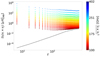 |
Fig. 1. Mean value over the Nsim simulations of the B-mode angular power spectra 𝒟ℓ(νi × νj) for the d1c simulation type, with rsim = 0. The color bar spans all the Ncross spectra 𝒟ℓ(νi × νj), associated to their reduced cross-frequency |

In order to avoid noise auto-correlation in the auto-spectra (i.e., 𝒟ℓ(νi × νj) when i = j), the latter are estimated in a way that differs slightly from what is presented in Sect. 3.2.3. We simulate two noise-independent data subsets at an observing frequency νi, with a noise amplitude  higher than that of the frequency band, and compute the cross-angular power spectrum between those. Thus, 𝒟ℓ(νi × νi) is free from noise auto-correlation bias at the expense of multiplying the noise amplitude in the spectrum by a factor of two. This approach is similar to that commonly used by the Planck Collaboration (see e.g., Planck Collaboration Int. XXX 2016; Planck Collaboration XI 2020; Tristram et al. 2021).
The spectra are evaluated in the multipole interval ℓ ∈ [1,200] in order to be able to focus on the reionization and recombination bumps of the primordial B-modes spectra. The spectra are binned in Nℓ = 20 bins of size Δℓ = 10 using NAMASTER. The same binning is applied throughout this article such that, in the following, the multipole ℓ denotes the multipole bin of size Δℓ = 10 centered on ℓ4.
From the sets of (Q,U) maps, NAMASTER computes the  ,
,  , and
, and  angular power spectra; for the sake of the present analysis, we keep only
  . Hence, when we discuss or analyze power spectra, we are referring to the B-mode power spectra
  . All spectra are expressed in (μKCMB)2.
4. Best-fit implementation
In order to characterize the complexity of the dust SED that will be measured by LiteBIRD, we modeled the angular power spectra of our simulations described in Sect. 3 over the whole frequency and multipole ranges with the moment expansion formalism introduced in Sect. 2.
4.1. General implementation
For each multipole ℓ, we ordered the angular power spectra  ) as in Eq. (16) in order to build a SED that is a function of both νi and νj. We fit this SED with models, as in Eq. (8) for example, using a Levenberg-Marquardt χ2 minimization with mpfit (Markwardt 2009)5. All the fits performed with mpfit were also realized with more computationally heavy Monte Carlo Markov chains (MCMC) with emcee (Foreman-Mackey et al. 2013), giving compatible results, well within the error bars.
The reduced χ2 minimization is given by

where Nd.o.f. is the number of degrees of freedom and ℂ is the covariance matrix of our Nsim simulations, represented in Fig. 2, of dimension (Nℓ · Ncross)2:

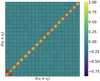 |
Fig. 2. Correlation matrix ( |

The entire covariance matrix ℂ is, in general, not invertible. To avoid this, we kept only the ℓ = ℓ′ block-diagonal of ℂ with the strongest correlation values6, as well as the (ℓ = 6.5,ℓ′ = 16.5) off-diagonal blocks showing a significant anti-correlation, as illustrated in Fig. 2. It was then possible to invert the thus-defined truncated correlation matrix with the required precision most of the time.
In the case of the d1 simulation type, we experienced a fit convergence issue for ∼ 20% of the simulations, leading to a very large χ2. In order to overcome this problem, two options lead to identical results: throwing away the outliers from the analysis or fitting using only the block-diagonal matrix (i.e., the ℓ = 6.5, ℓ′ = 16.5 block is set to zero). This last option solves the conversion issue while providing sufficient precision. The results presented in the following are using the block-diagonal matrix when the simulation type is d1.
Finally, in Eq. (17), R is the residual vector associated with every simulation of size Nℓ × Ncross:
with  .
.
The expression used for the model to fit is given by:
where Alens is not a free parameter and will remain fixed to zero (when there is no CMB, simulation types d0, d1T, and d1) or one (when the CMB is included, simulation types d0c, d1Tc and d1c). We leave the question of the impact of dust modeling with moments on the lensing measurement for future work. In Eq. (20), the free parameters can thus be β0(ℓ), T0(ℓ), and  and the tensor-to-scalar ratio r. The estimated value of r is referred to as
No priors on the parameters are used in order to explore the parameter space with minimal assumptions. Finally, a frequency-dependent conversion factor is included in  – from (MJy sr−1)2 to (μKCMB)2 – to express the dust spectra in (μKCMB)2 units. In those units,
  and
and  are frequency-independent.
To mitigate the impact of outliers in our simulations, all the final values of the best-fit parameters and χ2 distributions are represented by their median and median absolute deviations over Nsim values. For the tensor-to-scalar ratio  , we chose to represent all the best-fit values from the Nsim simulations in a histogram and we assume its distribution is normal. Fitting a Gaussian curve on this histogram and getting the mean and standard deviation gives us the final values of
  and
and  presented in the paper.
4.2. Implementation for the dust component
For the dust component, we consider four different fitting schemes, corresponding to four expressions for the dust model  in Eq. (20), which are referred to as “MBB”, “β-1”, “β-T”, and “β-2”. Each of them corresponds to a truncation of Eq. (8), keeping only some selected terms of the moment expansion: MBB stands for those of the modified black body, β-1 for those of the expansion in β at first order, β-2 for the expansion in β at second order, and β-T for the expansion in both β and T at first order. We chose the β-1 and β-2 truncations based on the studies of Mangilli et al. (2021) and Azzoni et al. (2021), where the dust SED moment expansion is performed only with respect to β. The β-T fitting scheme is instead the first-order truncation in both β and T, introduced here for the first time at the power spectrum level. The parameters fitted in each of these fitting schemes are summarized in Table 3. We note that the β-2 and β-T fitting schemes share the same number of free parameters. Finally, when we fit
  at the same time as the dust parameters, the fitting schemes will be referred to as rMBB, rβ-1, rβ-T, and rβ-2.
Different physical processes are expected to occur at different angular scales, leading to different SED properties. Thus, we estimate the dust-related parameters with one parameter per multipole bin. As an example, we estimate β0 = β0(ℓ) and T0 = T0(ℓ) to be able to take into account their scale dependence, at the cost of increasing the number of free parameters in our model. This is also true for the higher order moments. On the other hand,  is not scale dependent and, when it is fitted, we add one single parameter over the whole multipole range.
In Mangilli et al. (2021), the first-order moment expansion parameter  is considered to be the leading order correction to the MBB spectral index. We applied a similar approach in the present work, extending it to the dust temperature when it is fitted. In our pipeline, we proceed iteratively:
-
(i) we fit β0(ℓ) and T0(ℓ) at order zero (MBB), for each ℓ,
-
(ii) we fix β0(ℓ) and T0(ℓ) and fit the higher order parameters, as in Eq. (8), (iii) we update the β0(ℓ) to βcorr(ℓ) (and T0(ℓ) to Tcorr(ℓ) in the case of β-T) as:
-
(iv) and we iterate from (ii) fixing β0(ℓ) = βcorr(ℓ), until
 converges to be compatible with zero (and T0(ℓ) = Tcorr(ℓ), until
  converges to zero in the case of β-T).
We used three such iterations, which we found to be sufficient to guarantee the convergence. As the moment expansion is a nonorthogonal and incomplete basis (Chluba et al. 2017), this iterative process is performed to ensure that the expansions up to different orders share the same β0(ℓ) and T0(ℓ) with  and
and  .
.
5. Results
In this section, we present our evaluation of the best-fit parameters for the different fitting schemes presented in Sect. 4.1 on the B-mode cross-angular power spectra computed from the different simulation types presented in Sect. 3.3 and on the Galactic mask keeping fsky = 0.7, which is defined in Sect. 3.4.1. We first tested the simulation types containing only dust and noise in order to calibrate the dust complexity of our data sets in Sect. 5.1. We then used CMB only plus noise simulations to assess the minimal error on  in Sect. 5.2 and, finally, we explored the dust, CMB, and noise simulation types to assess the impact of the dust complexity on
  in Sect. 5.3.
5.1. Dust only
To evaluate the amplitude of the dust moment parameters contained in the dust simulations in the absence of CMB, we ran the fitting schemes presented in Sect. 4.1 in the three simulation types d0, d1T, and d1 presented in Sect. 3.3. In these cases, Alens and r in Eq. (20) are both fixed to zero and the fitted parameters are given in Table 3 for every fitting scheme.
5.1.1. d0
The d0 dust maps presented in Sect. 3.2 extrapolate between frequency bands with a MBB SED with constant parameters over the sky: βd0 = 1.54 and Td0 = 20 K. We performed the fit with the four fitting schemes presented in Sect. 4.1.
In Fig. 3 the values of the reduced χ2(ℓ) for each fitting scheme are displayed. For every fitting scheme (MBB, β-1, β-T and β-2), the reduced χ2 are close to 1 over the whole multipole range (slightly below 1 for the β-1, β-T and β-2 fitting scheme). This indicates that the MBB is a good fit to the cross-angular power spectra computed from the d0 maps with a spatially invariant MBB SED, as expected. Adding additional (higher order) parameters, such as with β-1, β-T and β-2, has no significant effect on the χ2.
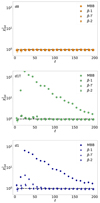 |
Fig. 3. Median of the reduced χ2 in every multipole bin ℓ, for all the Nsim simulations of d0 (top, orange), d1T (middle, green) and d1 (bottom, blue), on fsky = 0.7. The reduced χ2 values are reported for the four different fitting schemes: MBB (circles), β-1 (crosses), β-T (diamonds) and β-2 (triangles). The values for the four fitting schemes are shifted from each others by ℓ = 2, in order to distinguish them. The black dashed line represents |

In Fig. 4 we can see that the best-fit values of β0(ℓ) and T0(ℓ) are compatible with constant values β0(ℓ) = βd0 and T0(ℓ) = Td0, as expected for this simulated data set.
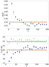 |
Fig. 4. Top: median of the best fit values of β0(ℓ) in d0 (orange), d1T (green), and d1 (blue) for the MBB (circles). βdo is marked by the dashed black line. Bottom: same as above but with T0(ℓ), the black dashed-lines being Td0 = 20 K and Td1T = 21.9 K. |
The best-fit values of the dust amplitude and the moment-expansion parameters are presented in Figs. 5–8, respectively. The amplitude power spectrum is compatible with that of the dust template map used to build d0 and the moment-xpansion parameters are compatible with zero for every fitting scheme, as expected with no spatial variation of the SED. Therefore, the moment expansion method presented in Sect. 2 passes the null test in the absence of SED distortions, with the d0 simulated data set.
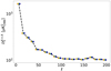 |
Fig. 5. Median of the best-fit values of |

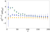 |
Fig. 6. Best-fit values of the first-order moment |

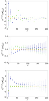 |
Fig. 7. Best-fit values of the second-order |


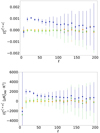 |
Fig. 8. Best-fit values of the first-order |


5.1.2. d1T
We now introduce, as a first layer of complexity, the spatial variations of the spectral index associated to a fixed temperature over the sky with the d1T simulation type. The dust temperature was fixed to Td1T = 21.9 K while the spectral index β(n) was allowed to vary between lines of sight. The four different fitting schemes presented in Sect. 4.1 are fitted over the cross-spectra of our simulations as in Sect. 5.1.1.
The reduced χ2(ℓ) values for each fitting scheme can be found in Fig. 3. It can be seen that the MBB no longer provides a good fit for the dust SED, especially at low multipoles. Averaging effects of spatially varying SEDs are more important over large angular scales and thus SED distortions and moments are expected to be more significant at low multipoles. Indeed, the moments added to the fit in β-1 are enough to lower the reduced χ2 such that it becomes compatible with 1 over almost all of the multipole range. The fitting schemes β-T and β-2, including more parameters than β-1, provide a fit of similar goodness, except in the multipole bin ℓ = 66.5 where they are closer to 1.
Figure 4 presents the best-fit values of β0(ℓ) in the case of the MBB fit. For the sake of clarity, the values after iteration (see Sect. 4.1) for β-1, β-T, and β-2 are not shown, but they present comparable trends. We can see that the best-fit values of β0(ℓ) for this d1T simulation type are no longer compatible with a constant. β0(ℓ) fitted values show a significant increase at low ( < 100) multipoles, up to β0 = (ℓ = 16.5) = 1.65. For ℓ > 100, β0(ℓ) is close to a constant of value ∼ 1.53. This increase towards the low ℓ is correlated to the increase of the MBB χ2 discussed in the previous paragraph. However, we note that in the lowest ℓ-bin, the β0(ℓ) value is close to 1.53 and that the χ2 of the MBB fit is close to unity.
The best-fit values of T0(ℓ) are also presented in Fig. 4 in the case of the MBB fit. Here again, the values after iteration for the other fitting schemes are not presented, but are similar. The d1TT0(ℓ) best-fit values oscillate around Td1T = 21.9 K, without being strictly compatible with a constant value, as would be expected for this simulation type. This tends to indicate that the SED distortions due to the spectral index spatial variations are affecting the accuracy at which we can recover the correct angular dependence of the sky temperature.
The amplitude power spectrum is displayed in Fig. 5 for the MBB fitting scheme. The other fitting scheme results are not presented for clarity and would not be distinguishable from those of the MBB. The fitted  is compatible with the one of the dust template map used to build the simulations.
All the parameters of the moment expansion with respect to β can be found in Figs. 6 and 7, and are now significantly detected, except for  . In Fig. 8, we can observe that the parameters of the moment expansion with respect to the temperature (only present in the β-T fit) remain undetected. The SED distortions due to the spatial variations of β are well detected, while no SED distortion linked to the temperature is seen, as expected for the d1T simulation type.
5.1.3. d1
We now discuss the d1 simulations, with the highest complexity in the polarized dust SED. In this more physically relevant simulation type, the dust emission is given by a MBB with variable index β(n) and temperature T(n) over the sky. We ran the four different fitting schemes on the d1 simulation type, as we did in Sects. 5.1.1 and 5.1.2.
The values of the reduced χ2(ℓ) are displayed in Fig. 3. For the MBB and β-1, the reduced χ2 are not compatible with unity, especially at low multipole. This indicates that none of them are a good fit anymore for the spatially varying SED with β(n) and T(n). With β-2 and β-T, the χ2(ℓ) values become compatible with unity, except for the ℓ = 26.5 bin. We note that β-T provides a slightly better fit than β-2 in this bin.
Looking at the medians of the best-fit values of β0(ℓ) for d1 in Fig. 4, we can see that the spectral index is changing with respect to ℓ, as discussed in Sect. 5.1.2, in a similar manner as for the d1T simulation type. The fitted temperature T0(ℓ) values for d1 show an increasing trend from ∼ 17 to ∼ 20.5 K and from ℓ = 16.5 to ℓ ∼ 100. At higher multipoles, T0(ℓ) is close to a constant temperature of 20.5 K. In d1, as for d1T, the angular scales at which we observe strong variations of β0(ℓ) and T0(ℓ) are the ones for which we observe a poor χ2 for some fitting schemes. Also, as for d1T, the largest angular scale ℓ-bin, at ℓ = 6.5, shows β and T values close to the constant value at high ℓ, which are associated with χ2 values closer to unity. The best-fit values of the amplitude  are shown in Fig. 5. These are similar to those of the other simulation types.
The moment-expansion parameters fitted on d1 are shown in Figs. 6–8. For this simulation type, the moment parameters are all significantly detected with respect to both β and T. This was already the case with the Planck intensity simulations, produced in a similar way, as discussed in Mangilli et al. (2021). Their detections quantify the complexity of dust emission and SED distortions from the MBB present in the d1 simulation type, due to the spatial variations of β(n) and T(n).
5.2. CMB only
In order to calibrate the accuracy at which the r parameter can be constrained with the LiteBIRD simulated data sets presented in Sect. 3.3, we tested the simulation type with no dust component,  , and with no tensor modes (rsim = 0, only CMB lensing and noise). We fit the expression in Eq. (20) with
  fixed to zero and Alens fixed to one (i.e., r is the only parameter we fit in this case). Doing so over the Nsim simulations, we obtain
  . This sets the minimal value we can expect to retrieve for
  with our assumptions if the dust component is perfectly taken into account.
5.3. Dust and CMB
We now present our analysis of the simulations including dust, CMB (lensing), and noise (d0c, d1Tc and d1c) with no primordial tensor modes (rsim = 0). As described above, we applied the four fitting schemes for the dust on the three simulation types, fitting  and fixing Alens to one (namely rMBB, rβ-1, rβ-T and rβ-2) simultaneously.
The best-fit values of β0(ℓ), T0(ℓ) and the moment expansion parameters  derived with the simulation types d0c, d1Tc, and d1c are not discussed further when they are compatible with the ones obtained for the d0, d1T, and d1 simulation types and presented in Sect. 5.1.
5.3.1. d0c
For d0c, as for d0, we recover the input constant spectral index and temperature βd0 and Td0 at all angular scales for every fitting scheme. Furthermore, we do not detect any moment, when fitting rβ-1, rβ-T, and rβ-2. This simulation type therefore constitutes our null-test when  and the dust parameters are fitted at the same time. The addition of the CMB lensing in the simulations and the addition of r to the fits thus does not lead to the detection of the moment parameters nor biases the recovery of the spectral index and the temperature.
The posterior distributions of the estimated tensor-to-scalar ratio  are displayed in Fig. 9 and their mean and standard deviations are summarized in Table 4. We note that
  is compatible with the input value (rsim = 0) for all the fitting schemes. For rMBB and rβ-1, the dispersion
  is comparable with the CMB-only scenario discussed in Sect. 5.2. For rβ-T and rβ-2, the width of the distribution increases by a factor of ∼ 2 and ∼ 4, respectively.
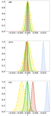 |
Fig. 9. Top panel: posterior on |

Best-fit values of  in units of 10−4 on fsky = 0.7.
5.3.2. d1Tc
The posterior distribution of  in the case of the d1Tc simulation type is displayed in Fig. 9 for the four fitting schemes and the mean value and standard deviation of these distributions are summarized in Table 4. We can see that in the case of rMBB, we fit
  . In that case, the input tensor-to-scalar ratio rsim = 0 is not recovered and we obtain a bias on the central value of
  of
of  . As discussed in Sect. 2.1.2, this is expected because we know that the MBB is not a good dust model for a SED with spatially varying spectral index, as we also verify in Sect. 5.1.2 looking at the χ2 values.
Using the rβ-1 fitting scheme allows us to recover  , where rsim is recovered within
  , while rβ-2 and rβ-T recover the input value within
  (with
(with  and
and  , respectively). As in Sect. 5.3.1, the deviation remains similar between rMBB and rβ-1 and increases by a factor of ∼ 2 and ∼ 4 from rβ-1 to rβ-T and rβ-2, respectively.
5.3.3. d1c
In the case of the d1c simulation type, as in d0c and d1Tc, we fit  in addition to the dust-related parameters. In that case, dust moment parameters are recovered as for d1 (see Sect. 5.1.3), except for the rβ-2 fitting scheme.
Figure A.2 compares the moment parameters between β-2 on the d1c simulations type, fitting only the dust-related parameters and rβ-2 on d1c when jointly fitting the dust parameters and  . We observe that
  is not consistently recovered when fitting
  in addition to the dust parameters.
A similar comparison can be found in Fig. A.3 for the moment parameters between β-T and rβ-T on the d1c simulation type. Using this fitting scheme, we can see that all the moments are correctly recovered when adding  to the fit.
The  posterior distributions in the case of d1c are displayed in Fig. 9 and summarized in Table 4. As discussed in Sect. 2.1.2 and observed in Sect. 5.3.3, the rMBB fit is highly biased, with
  (by more than 21
  ). When fitting the rβ-1, this bias is significantly reduced (
 ,
,  away from rsim = 0), illustrating the ability of the first-moment parameters to correctly capture part of the SED complexity. However, performing the expansion in both β and T with rβ-T allows us to recover rsim without bias (
 ), highlighting the need for the description of the SED complexity in terms of dust temperature for this simulated data set where both β and T vary spatially. On the other hand, for rβ-2, a negative tension (
 ) can be observed:
  . This tension is discussed in Sect. 6.5.
For d1c, the  distribution widths roughly meet the foreground cleaning requirements of LiteBIRD presented in Sect. 3.1 for rMBB and rβ-1 but are higher for rβ-T and rβ-2. We also note that, with the same number of free parameters, all the standard deviations
  slightly increase compared to the d0c simulation type. This is expected due to the increasing dust complexity.
6. Discussion
6.1. Lessons learnt
In Sect. 5, we apply the fitting pipeline introduced in Sect. 4 on LiteBIRD simulated data sets on fsky = 0.7 and for rsim = 0, including the various dust simulation types defined in Sect. 3.2. We fitted the estimated B-mode power-spectra with the four different fitting schemes summarized in Table 3. Our main results can be summarized as follows:
-
The MBB fitting scheme provides a good fit for the dust component in the d0 and d0c simulation types. However, when the spectral index changes with the angular scale, such as in the d1T, d1Tc, d1, and d1c simulations, this approach no longer provides a good fit because of the complexity of the dust SED. As a consequence, in the rMBB case, rsim cannot be recovered without a significant bias.
-
The β-1 fitting scheme allows us to perform a good fit for the dust complexity using the d0 and d1T simulations but not for d1, while the rβ-1 fitting scheme yields estimates of
 close to rsim within
  for d0c, and within
  for d1Tc, but presenting a bias of
  for d1c.
 -
The β-T fitting scheme provides a good fit for every dust model, while using the rβ-T fitting scheme allows us to recover
 values consistent with rsim within
  for all the simulation types, but is associated with an increase of
  by a factor ∼ 2 compared to the rβ-1 case.
 -
The β-2 fitting scheme also provides a good fit for each dust model, and the rβ-2 fitting scheme leads to values of
 compatible with rsim within
  for all the simulation types but d1c. In this last case, there is a negative tension of
  . For all the simulation types, there is an increase of
  by a factor of ∼ 4 compared to the rβ-1 case.
The present analysis shows that the temperature could be a critical parameter for the moment expansion in the context of LiteBIRD.
Indeed, for simulations including a dust component with a spectral index and a temperature that both vary spatially, as in d1, the only fitting scheme allowing us to recover rsim within  is rβ-T, the expansion to first order in both β and T. This shows that expanding in β only, without treating T, is not satisfactory when looking at such large fractions of the sky. Indeed, when applying the β-2 fitting scheme, the
  parameter remains undetected for the d1T simulation type (Sect. 5.1.2), while it is significantly detected using the d1 simulation type (Sect. 5.1.3). Nevertheless, d1T and d1share the same template of β(n) (Sect. 3.2) and they only differ by the sky temperature (constant for d1T and varying for d1). This suggests that the observed
  with the d1 simulations originates from the temperature variations and not those in the spectral index. This observation shows that it is less convenient to use the β-2 fitting scheme than the β-T one in order to correctly recover the moment-expansion parameters and
  when temperature varies spatially.
Moreover, we saw that  is lower when using the fitting scheme rβ-T instead of rβ-2 for every simulation type, even if both have the same number of free parameters. This second observation additionally encourages an approach where the SED is expanded with respect to both β and T. Nevertheless, the uncertainty on
  we obtain in this case (
 ) is larger than the LiteBIRD requirements.
6.2. Increasing the accuracy on the tensor-to-scalar ratio
In Sect. 5.1.3 and Fig. 3, we see that the MBB and β-1 fitting schemes do not provide good fits for the d1 dust simulations, especially at low multipoles (ℓ ≲ 100). Conjointly, in Fig. 8, we can see that the β-T moment parameters are significantly detected for ℓ ≲ 100 and compatible with zero above that threshold, suggesting that their corrections to the SED are predominantly required at large angular scales.
This implies that we can improve the pipeline presented in Sect. 4 to keep only the required parameters in order to recover  compatible with rsim with a minimal
  . It can be achieved by applying the rβ-1 fitting sheme over the whole multipole range, while restricting the rβ-T-specific (
 and
and  ) moment-expansion parameters fit to the low multipoles range. We note that in order to correct the bias, it is still necessary to keep the rβ-1 moment parameters even at high multipoles, because the MBB does not provide a good fit even for ℓ ∈ [100,200], as we can see in Fig. 3. We define ℓcut as the multipole bin under which we keep all the rβ-T moment parameters and above which we use the rβ-1 scheme.
The best-fit values and standard deviations of  for different values of ℓcut are displayed in Table 5. We can see that a trade-off has to be found: the smaller the ℓcut, the bigger the shift from rsim, and the bigger the ℓcut, the higher the value of
  . The trade-off point seems to be found for ℓcut, allowing us to recover
  without tension, with
  . The error on r is thus reduced by more than ∼ 30% with respect to the nonoptimized fit and meets the LiteBIRD requirements.
Best-fit values of  in units of 10−4 for different values of ℓcut for the d1c simulations with fsky = 0.7, when applying the rβ-T fitting scheme.
6.3. Tests with smaller sky fractions
In all the results presented in Sect. 5, we were considering a sky fraction of fsky = 0.7. This sky mask keeps a considerable fraction of the brightest Galactic dust emission. To quantify the impact of the sky fraction on our analysis, we ran the pipeline as in Sect. 5.3.3 with the different masks introduced in Sect. 3.4.1 (fsky = 0.5 and fsky = 0.6). This was done with the d1c simulation type.
The posteriors on  for the different fitting schemes are displayed in Fig. 10 and Table 6. We can see that, while the rMBB fiting scheme always leads to biased estimates, the rβ-1 case allows us to recover
  at
at  for fsky = 0.5 and within
  for fsky = 0.6. In the two situations, the results using the rβ-T and β-2 fitting schemes are both unbiased with estimates of
  compatible with rsim within
  . The
. The  hierarchy between the rMBB, rβ-1, rβ-T, and rβ-2 fitting schemes is the same as for fsky = 0.7 (see Sect. 5.3.3). Nevertheless, we observe that
  increases as the sky fraction decreases, as does the statistical error (cosmic variance of the lensing and noise). The bias, on the other hand, decreases for all the fitting schemes with the sky fraction, which is expected because less dust emission contributes to the angular power spectra. The negative tension observed on the
  posterior in Sect. 5.3.3 for the rβ-2 case is not present when using smaller sky fractions. In Fig. A.5, the rβ-2 moment parameters are displayed. We can see that they are not significantly detected for the fsky = 0.5 and 0.6, unlike for fsky = 0.7. As we have seen that some of the moments in the β-2 fitting scheme failed to model SED distortions coming from temperature, we can suppose that, in our simulations, the temperature variations play a less significant role in the dust SED on the fsky = 0.5 and 0.6 masks than they play in the fsky = 0.7 one. As a consequence, they have a smaller impact on r when not properly taken into account.
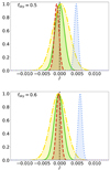 |
Fig. 10. Top panel: posterior on |

Best-fit values of  in units of 10−4 for an alternative d1c simulation with rsim = 0.01 on fsky = 0.7, and with rsim = 0 but on fsky = 0.5 and fsky = 0.6.
6.4. Tests with nonzero input tensor modes
We show in Sect. 5.3.3 that the rβ-T fitting scheme allows us to retrieve  compatible with zero when rsim = 0. We now want to assess the potential leakage of
  in the moment expansion parameters if rsim ≠ 0. In this case, primordial tensor signals would be incorrectly interpreted as dust complexity. We run the pipeline as described in Sect. 5.3.3 with rsim = 0.01, in the d1c simulation type. This value of rsim = 0.01 is larger than the value targeted by LiteBIRD, but given the order of magnitude of the error on
  observed in the previous sections, a potential leakage could be left unnoticed using a smaller rsim.
Looking at the final posterior on  (Fig. 11 and Table 6), we can see that the results are comparable with the rsim = 0 case, but centered on the new input value rsim = 0.01. The rMBB fitting scheme gives a highly biased posterior of
  ; the bias is reduced but still significant when using the rβ-1 scheme (
 ); in the β-T case we get an estimate of
  compatible with the input value of rsim = 100 × 10−4; and finally, the β-2 fitting scheme leads to a negative
  tension (
 ). This demonstrates the robustness of our method and its potential application to component separation. We note that the negative bias at second order is still present in the rsim = 0.01 case, illustrating that setting a positive prior on
  would not have been a satisfying solution when rsim = 0.
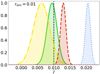 |
Fig. 11. Posterior on |

6.5. Exploring the correlations between the parameters
We now examine the substantial increase in the dispersion on the  posteriors between the rβ-1 fitting scheme on the one hand and the rβ-T and rβ-2 ones on the other. Indeed, in Sect. 5.3.3, we show that
  is about two times greater when using the rβ-T scheme than the rβ-1 one, and about four times larger in the case of rβ-2, while the rβ-T and rβ-2 schemes share the same number of free parameters. Some other points to clarify are the shift on
  appearing for rβ-2 in the d1c scenario, discussed in Sect. 5.3.3, and the inability to correctly recover
  when
when  is added to the fit illustrated in Fig. A.2.
The 2D-SED shapes of the parameters  in the (νi,νj) space7 are displayed in Fig. A.4. We used the nine frequencies of LiteBIRD presented in Sect. 3.2.3 and fixed β0 = 1.54 and T0 = 20 K. We also introduce the CMB 2D-SED shape with the black body function:
where TCMB = 2.726 K.
The 2D correlation coefficients between these 2D-SED shapes are displayed in Fig. 12. We present the correlations between the shapes of the parameters in the case of the rβ-T and rβ-2 fitting schemes. We can see that all the moment parameters in  are strongly correlated with the CMB SED signal, while the ones in
  are not.
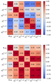 |
Fig. 12. Correlation matrices of the 2D-SED shapes of the CMB (BCMB(νi × νj) and dust moments |

We showed that, when fitting β-2 on d1c, the SED distortions due to spatial variations of T are incorrectly detected by the second-order moment parameters with respect to the spectral index β. Due to the correlations highlighted above, those spurious moment parameters could then leak into  when adding it to the fit in rβ-2. This explains both the negative shift on the
  posterior using β-2 in the d1c simulation type with fsky = 0.7 presented in Sects. 5.3.3 and 6.4, and the inability to correctly recover the
  dust moment parameter presented in Fig. A.2. In addition, it gives a natural reason for the surge of
  when the second-order moments in β are added to the fit.
On the other hand, the moment parameters in  are strongly correlated with the moments in
  . This behavior is expected due to the strong correlation between β and T (see e.g., Juvela & Ysard 2012). However those moment parameters are less correlated with the CMB signal than the second-order parameters of β-2. This points out that the factor of ∼ 2 on
  between β-T and β-2 is due to this correlation of the 2D-SED shapes. As the parameters in
  are highly correlated with one another, we expect them to be highly redundant in the fit. However, repeating the process described in Sect. 5.3.3 using only
  for β-T –which is equivalent to applying the β-1 fitting scheme with an iterative correction to the temperature T0(ℓ)– gives a
  posterior similar to the one obtained for β-1 alone. Taking the other
  terms into account appears to be necessary in order to recover an unbiased distribution of
  .
.
6.6. Adding synchrotron to the simulations
Thermal dust is not the only source of polarized foreground that must be considered for CMB studies. Although subdominant at high frequencies (≥ 100 GHz), the synchrotron emission due to accelerated electrons in the interstellar medium is still expected to represent a significant fraction of the total polarized signal.
In order to take one more step towards realistic forecasts for the LiteBIRD instrument, we add a synchrotron contribution to the d1c simulations presented in Sect. 3.3 using the s1 template included in the PYSM. In this scenario, the synchrotron SED for each line of sight is given by a power law of the form (in antenna temperature units)
where the amplitude As1(n) and the spectral index βs1(n) maps are derived from the combination of the WMAP mission 23 GHz map Bennett et al. (2013) and Haslam 408 GHz map Haslam et al. (1981).  is defined as 23 GHz. The simulations containing synchrotron are referred to as d1s1c below.
If not treated in the fit, the presence of synchrotron is expected to induce a bias on the  posterior distribution. Regarding the dust MBB discussed in Sect. 2.1.2, the synchrotron SED is expected to have distortions. However, as the synchrotron polarized emission is significantly lower than that of dust, in the frequency range considered in the present work, we expect the distortions to be small compared to the ones induced by dust and we leave their modeling to a further study.
In order to minimize the number of free parameters used for fitting the synchrotron emission, we model its power spectrum as a power law of the multipole ℓ (Krachmalnicoff et al. 2018). Therefore, combining with the synchrotron SED in Eq. (23), the synchrotron component of the cross-angular power spectra reads
where the amplitude coefficient As is treated as a free parameter while we fix βs = −3 (median value of the s1 βs map on our fsky = 0.7 mask) and αs = −1 (Krachmalnicoff et al. 2018).
When fitting the d1s1c simulations, we either use the rβ-T fitting scheme, neglecting the synchrotron component, or we add the synchrotron component in Eq. (24) to the model in Eq. (20). We refer to this latter case as the srβ-T fitting scheme. In Fig. 13, the  posteriors derived from the d1s1c simulations are displayed with rsim = 0 and fsky = 0.7.
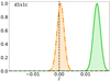 |
Fig. 13. Posterior on |

Using the rβ-T fitting scheme, we find  . As expected, even at high frequencies, modeling the synchrotron component is critical and cannot be neglected in order to recover an unbiased value of
  . On the other hand, using srβ-T fitting scheme, we recover
  . This result is comparable with the one obtained for the d1c simulations in Sect. 5.3.3, with a minor increase in
  . We can therefore conclude that a model as simple as that of Eq. (24) is sufficient to take into account the s1 component at ν > 100 GHz and the corresponding SED distortions can be neglected in order to recover an unbiased value of
  . In principle, as we know that the dust-synchrotron spatial correlation is significant at large scales (Planck Collaboration XI 2020), Eq. (20) should include a dust-synchrotron term (see e.g., Hensley et al. 2021). In our study, where we consider cross-spectra from 100 to 402 GHz, this dust-synchrotron term is subdominant, but it could be significant when considering cross-spectra between LiteBIRD’s extreme frequency bands (e.g., the 40 × 402 cross-spectrum). The moment expansion might be more complicated as well in this case, as we could expect some correlation between the dust and synchrotron moment-terms.
This result shows that a full polarized foreground content can be treated at high frequencies when using a power law SED for the synchrotron coupled with the moment expansion of the MBB up to first order in both β and T for the dust SED. A full study remains to be done in that direction using all the frequency bands of the LiteBIRD instrument. Eventually, Eq. (24) will also have to be expanded in moments with respect to its parameters. Doing so, one can expect to recover an unbiased value of  associated with a decrease in
  down to a value compatible with the full success criterion of the mission.
6.7. Limitations of this work and caveats
As discussed in Sect. 2.2.1, we neglected polarization effects through this work by treating the BB signal as an intensity signal. This is not problematic in the present work, because no variations along the lines of sight were present in the simulations. However, this point has to be addressed using complex simulations or real sky data.
The choice of reference frequency ν0 used for the normalization of the MBB in Eq. (1), which is not discussed in this study, can potentially have a significant impact on the moment expansion and, in turn, on the measurement of  . Indeed, ν0 is the pivot frequency of the moment expansion (moments are equal to zero at ν0) and will determine the shape of the SED distortion around it. A poor choice for this reference frequency can have disastrous consequences for the moment fit: for example, if it is chosen far away from the observed bands, all the moments will become degenerated. In our case, the reference frequency (353 GHz) is within the observed frequency range (100 − 402 GHz), but we have not tried to optimize its position. In addition, the ν0 pivot of our moment expansion coincides with the one used to extrapolate the dust template map in the PYSM and we have not quantified how much this impacts our results.
Finally, as pointed out several times in this work, the quantitative results depend strongly on the sky model of our simulations. Moreover, we lack dedicated sky models where we can control the complexity of the dust SED, either by directly including moments or by averaging the emission from the 3D structure of the Galaxy. However, both methods are beyond the scope of the present work.
7. Conclusion
Being able to precisely characterize the complexity of the Galactic thermal dust polarized SED has become critical for the measurement of the faint primordial B-mode signal of the CMB, especially at the sensitivity targeted by future CMB experiments such as the LiteBIRD satellite mission.
In this work, we applied the moment expansion formalism to the dust emission SED as a component-separation tool to recover the tensor-to-scalar ratio parameter r in LiteBIRD-simulated data. This formalism, proposed by Chluba et al. (2017) and implemented in harmonic space by Mangilli et al. (2021), allows us to deal with the spectral complexity of the Galactic dust signal by modeling its deviations from the canonical MBB model at the cross-angular power spectrum level. In the case of the data-driven realistic dust emission model –we explore (PYSM d1) here–, suitably taking into account the dust SED distortions prevents the spurious detection of the primordial B-mode signal.
We show that the dust spectral index β and dust temperature T spatial variations significantly distort the dust cross-power spectrum SED. The MBB is not a good model to describe the data in that case and the estimation of r is dramatically affected. In the case where no primordial signal is included in the simulated data sets, not taking into account the dust SED complexity leads to a highly significant spurious detection of r with LiteBIRD (from  to 1.25 × 10⁻², with a 8.4 to 21.2σ significance, from 50 to 70% of the sky, respectively).
To overcome this obstacle, we applied the moment expansion formalism in order to model these SED distortions. We demonstrate that, at LiteBIRD sensitivity, the previously studied moment expansion with respect to the dust spectral index β (Mangilli et al. 2021; Azzoni et al. 2021) does not give satisfactory results. Indeed, expanding in β to first order (following the angular power spectrum definition of the order) leads to a significant bias on 70% of the sky ( when rsim = 0 and
  , when rsim = 10−2). At second order in β, we observe a ∼ 2 σ negative tension (
 when rsim = 0 and
  , when rsim = 10−2).
We introduce for the first time in this work the expansion of the dust angular cross-power spectra with respect to both β and T. We show that by using this expansion up to first order, we correctly model the dust SED distortions due to spatial variations of both β and T at the map level. This allows us to recover r parameter without bias, with  if rsim = 0 and
  if rsim = 10−2. Thus, despite the known degeneracy between the dust spectral index and its temperature in the Rayleigh-Jeans domain, it is important to correctly model the latter in order to accurately retrieve the tensor-to-scalar ratio r at the unprecedented precision reached by experiments such as LiteBIRD.
Adding parameters to tackle the dust SED complexity means an increase in the error budget. Given the LiteBIRD bands and sensitivities we consider in this work (frequency bands above 100 GHz), the ideal sensitivity on r without delensing is  . In the ideal case, where the dust β and T are constant over the sky (PYSM d0), separating the CMB from dust leads to
  on 70% of the sky. Adding the expansion to first order in β does not significantly increase the error (
 ), but expanding to first order in both β and T multiplies it by a factor of ∼ 2 (
 ) and to second order in β by a factor of ∼ 4 (
 ). We show that the surge of
  between the two latter cases, sharing the same number of free parameters, is due to strong correlations between the SED of the second-order moments in β and the CMB. This is an important point, as it could lead to some intrinsic limitation for component-separation algorithms based exclusively on the modeling of the SED. Furthermore, when dealing with real data, if the dust SED is complex enough to have significant second-order distortions with respect to β, CMB experiments might reach a dilemma: either include the second order in the modeling at the cost of losing sensitivity on r, or neglect it at the cost of a potential spurious detection. Coupling the SED-based separation with methods exploiting the diversity of spatial distribution between components (e.g., Regaldo-Saint Blancard et al. 2021) seems a natural way to overcome this issue.
Nevertheless, moment expansion at the cross-angular power spectrum level provides a powerful and agnostic tool, allowing us to analytically recover the actual dust complexity without making any further assumptions. We additionally show that this method is robust, in the sense that it can effectively distinguish the primordial tensor signal from dust when rsim ≠ 0, as in the case of LiteBIRD simulations. The dust moments in β and T at first order are needed in order to retrieve a reliable measure of r; they are significantly detected for ℓ ≲ 100. We can therefore define a cut in ℓ above which we do not fit for the whole complexity of the dust (we fit only the expansion up to first order in β and not in β and T). Doing so, we can reduce the error on  while keeping the bias negligible (
 ). We could imagine other ways to reduce the number of free parameters in our model (e.g., assuming a power-law of ℓ behavior for the moments, as in Azzoni et al. 2021) and hence reduce the error on r. However, this optimization really depends on the simulated sky complexity and has not been comprehensively explored in the present work.
The PYSM d1 sky simulations, being data-driven, are widely used by the CMB community as they contain some of the real sky complexity. Nevertheless, at high-Galactic latitudes, the dust spectral index and temperature templates from Planck are dominated by systematic errors (uncertainty on the assumed zero-level of the Planck intensity maps, residual cosmic infrared background (CIB), anisotropies, instrumental noise, etc.). Therefore, some of the complexity we observe far from the Galactic plane in this sky model is not real. On the other hand, the modeled SED of the dust is exactly a MBB in each pixel, and line-of-sight averages or more complex dust models are ignored. As a consequence, our method and CMB B-mode component-separation algorithms in general need to be confronted with more complex models in order to really assess their performances in a quantitative manner.
Finally, although we demonstrate that the synchrotron component can be tackled at frequencies above 100 GHz with a minimal model under our assumptions, a study over the full LiteBIRD frequency bands, including synchrotron and the potential moment expansion of its SED, will be considered as a natural next step for a further application.
For example, ![$ {\mathcal{S} }(\nu _i,\nu _j) = \frac{I_{\nu _i}(\beta _0,T_0)I_{\nu _j}(\beta _0,T_0)}{I_{\nu _0}(\beta _0,T_0)^2}\cdot \left[\ln \left(\frac{\nu _i}{\nu _0}\right)\ln \left(\frac{\nu _j}{\nu _0}\right) \right] $](/articles/aa/full_html/2022/04/aa42664-21/aa42664-21-eq249.gif) is associated to the
is associated to the  parameter (see Eq. (8)).
Acknowledgments
This work is supported in Japan by ISAS/JAXA for Pre-Phase A2 studies, by the acceleration program of JAXA research and development directorate, by the World Premier International Research Center Initiative (WPI) of MEXT, by the JSPS Core-to-Core Program of A. Advanced Research Networks, and by JSPS KAKENHI Grant Numbers JP15H05891, JP17H01115, and JP17H01125. The Italian LiteBIRD phase A contribution is supported by the Italian Space Agency (ASI Grants No. 2020-9-HH.0 and 2016-24-H.1-2018), the National Institute for Nuclear Physics (INFN) and the National Institute for Astrophysics (INAF). The French LiteBIRD phase A contribution is supported by the Centre National d’Etudes Spatiale (CNES), by the Centre National de la Recherche Scientifique (CNRS), and by the Commissariat à l’Energie Atomique (CEA). The Canadian contribution is supported by the Canadian Space Agency. The US contribution is supported by NASA grant no. 80NSSC18K0132. Norwegian participation in LiteBIRD is supported by the Research Council of Norway (Grant No. 263011). The Spanish LiteBIRD phase A contribution is supported by the Spanish Agencia Estatal de Investigación (AEI), project refs. PID2019-110610RB-C21 and AYA2017-84185-P. Funds that support the Swedish contributions come from the Swedish National Space Agency (SNSA/Rymdstyrelsen) and the Swedish Research Council (Reg. no. 2019-03959). The German participation in LiteBIRD is supported in part by the Excellence Cluster ORIGINS, which is funded by the Deutsche Forschungsgemeinschaft (DFG, German Research Foundation) under Germany’s Excellence Strategy (Grant No. EXC-2094 – 390783311). This research used resources of the Central Computing System owned and operated by the Computing Research Center at KEK, as well as resources of the National Energy Research Scientific Computing Center, a DOE Office of Science User Facility supported by the Office of Science of the US Department of Energy. M.R. acknowledges funding support from the ERC Consolidator Grant CMBSPEC (No. 725456) under the European Union’s Horizon 2020 research and innovation program. The authors would like to thank David Alonso, Josquin Errard, Nicoletta Krachmalnicoff and Giuseppe Puglisi, for useful discussions as well as Jens Chluba for insightful comments on earlier version of this work.
References
- Adak, D. 2021, MNRAS, 507, 4618 [NASA ADS] [CrossRef] [Google Scholar]
- Alonso, D., Sanchez, J., Slosar, A., & LSST Dark Energy Science Collaboration 2019, MNRAS, 484, 4127 [NASA ADS] [CrossRef] [Google Scholar]
- Ashton, P. C., Ade, P. A. R., Angilè, F. E., et al. 2018, ApJ, 857, 10 [Google Scholar]
- Azzoni, S., Abitbol, M. H., Alonso, D., et al. 2021, JCAP, 2021, 047 [CrossRef] [Google Scholar]
- Bennett, C. L., Larson, D., Weiland, J. L., et al. 2013, ApJS, 208, 20 [Google Scholar]
- BICEP2 Collaboration & Keck Array Collaboration 2018, Phys. Rev. Lett., 121, 221301 [Google Scholar]
- BICEP2/Keck& Planck Collaboration 2015, Phys. Rev. Lett., 114, 101301 [Google Scholar]
- Bicep/Keck Collaboration (Ade, P. A. R., et al.) 2021, Phys. Rev. Lett., 127, 151301 [NASA ADS] [CrossRef] [Google Scholar]
- Brout, R., Englert, F., & Gunzig, E. 1978, Ann. Phys., 115, 78 [Google Scholar]
- Chluba, J., Hill, J. C., & Abitbol, M. H. 2017, MNRAS, 472, 1195 [NASA ADS] [CrossRef] [Google Scholar]
- Desert, F. X., Boulanger, F., & Puget, J. L. 1990, A&A, 500, 313 [Google Scholar]
- Draine, B. T., & Hensley, B. 2013, ApJ, 765, 159 [Google Scholar]
- Fanciullo, L., Guillet, V., Aniano, G., et al. 2015, A&A, 580, A136 [NASA ADS] [CrossRef] [EDP Sciences] [Google Scholar]
- Foreman-Mackey, D., Hogg, D. W., Lang, D., & Goodman, J. 2013, PASP, 125, 306 [Google Scholar]
- Gandilo, N. N., Ade, P. A. R., Angilè, F. E., et al. 2016, ApJ, 824, 84 [Google Scholar]
- Górski, K. M., Hivon, E., Banday, A. J., et al. 2005, ApJ, 622, 759 [Google Scholar]
- Guillet, V., Fanciullo, L., Verstraete, L., et al. 2018, A&A, 610, A16 [NASA ADS] [CrossRef] [EDP Sciences] [Google Scholar]
- Guth, A. H. 1981, Phys. Rev. D, 23, 347 [Google Scholar]
- Haslam, C. G. T., Klein, U., Salter, C. J., et al. 1981, A&A, 100, 209 [NASA ADS] [Google Scholar]
- Hazumi, M. 2018, Frontier Research in Astrophysics – III, 79 [Google Scholar]
- Hazumi, M., Ade, P. A. R., & Adler, A. 2020, SPIE Conf. Ser., 11443, 114432F [Google Scholar]
- Hensley, B. S., & Bull, P. 2018, ApJ, 853, 127 [NASA ADS] [CrossRef] [Google Scholar]
- Hensley, B. S., Clark, S. E., Fanfani, V., et al. 2021, AAS J., submitted [arXiv:2111.02425] [Google Scholar]
- Hutton, S., Ferreras, I., & Yershov, V. 2015, MNRAS, 452, 1412 [NASA ADS] [CrossRef] [Google Scholar]
- Ichiki, K., Kanai, H., Katayama, N., & Komatsu, E. 2019, Progr. Theor. Exp. Phys., 2019, 033E01 [CrossRef] [Google Scholar]
- Juvela, M., & Ysard, N. 2012, A&A, 539, A71 [NASA ADS] [CrossRef] [EDP Sciences] [Google Scholar]
- Kamionkowski, M., Kosowsky, A., & Stebbins, A. 1997, Phys. Rev. Lett., 78, 2058 [Google Scholar]
- Krachmalnicoff, N., Baccigalupi, C., Aumont, J., Bersanelli, M., & Mennella, A. 2016, A&A, 588, A65 [NASA ADS] [CrossRef] [EDP Sciences] [Google Scholar]
- Krachmalnicoff, N., Carretti, E., Baccigalupi, C., et al. 2018, A&A, 618, A166 [NASA ADS] [CrossRef] [EDP Sciences] [Google Scholar]
- Lewis, A., Challinor, A., & Lasenby, A. 2000, ApJ, 538, 473 [Google Scholar]
- LiteBIRD Collaboration 2020, J. Low Temp. Phys., 199, 1107 [CrossRef] [Google Scholar]
- LiteBIRD Collaboration 2021, Proc. SPIE, 11443, 114432F [Google Scholar]
- Lyth, D. H. 1997, Phys. Rev. Lett., 78, 1861 [NASA ADS] [CrossRef] [Google Scholar]
- Mangilli, A., Aumont, J., Rotti, A., et al. 2021, A&A, 647, A52 [NASA ADS] [CrossRef] [EDP Sciences] [Google Scholar]
- Markwardt, C. B. 2009, in Astronomical Data Analysis Software and Systems XVIII, eds. D. A. Bohlender, D. Durand, & P. Dowler, ASP Conf. Ser., 411, 251 [Google Scholar]
- Martin, J., Ringeval, C., & Vennin, V. 2014, Phys. Dark Univ., 5, 75 [CrossRef] [Google Scholar]
- Paradis, D., Bernard, J. P., & Mény, C. 2009, A&A, 506, 745 [NASA ADS] [CrossRef] [EDP Sciences] [Google Scholar]
- Pelgrims, V., Clark, S. E., Hensley, B. S., et al. 2021, A&A, 647, A16 [NASA ADS] [CrossRef] [EDP Sciences] [Google Scholar]
- Planck Collaboration XI. 2014, A&A, 571, A11 [NASA ADS] [CrossRef] [EDP Sciences] [Google Scholar]
- Planck Collaboration Int. XVII. 2014, A&A, 566, A55 [NASA ADS] [CrossRef] [EDP Sciences] [Google Scholar]
- Planck Collaboration Int. XXII. 2015, A&A, 576, A107 [NASA ADS] [CrossRef] [EDP Sciences] [Google Scholar]
- Planck Collaboration I. 2016, A&A, 594, A1 [NASA ADS] [CrossRef] [EDP Sciences] [Google Scholar]
- Planck Collaboration X. 2016, A&A, 594, A10 [NASA ADS] [CrossRef] [EDP Sciences] [Google Scholar]
- Planck Collaboration Int. XXX. 2016, A&A, 586, A133 [NASA ADS] [CrossRef] [EDP Sciences] [Google Scholar]
- Planck Collaboration Int. L. 2017, A&A, 599, A51 [NASA ADS] [CrossRef] [EDP Sciences] [Google Scholar]
- Planck Collaboration I. 2020, A&A, 641, A1 [NASA ADS] [CrossRef] [EDP Sciences] [Google Scholar]
- Planck Collaboration IV. 2020, A&A, 641, A4 [NASA ADS] [CrossRef] [EDP Sciences] [Google Scholar]
- Planck Collaboration XI. 2020, A&A, 641, A11 [NASA ADS] [CrossRef] [EDP Sciences] [Google Scholar]
- Polnarev, A. G. 1985, Sov. Astron., 29, 607 [Google Scholar]
- Regaldo-Saint Blancard, B., Allys, E., Boulanger, F., Levrier, F., & Jeffrey, N. 2021, A&A, 649, L18 [NASA ADS] [CrossRef] [EDP Sciences] [Google Scholar]
- Remazeilles, M., Dickinson, C., Eriksen, H. K. K., & Wehus, I. K. 2016, MNRAS, 458, 2032 [Google Scholar]
- Remazeilles, M., Rotti, A., & Chluba, J. 2021, MNRAS, 503, 2478 [NASA ADS] [CrossRef] [Google Scholar]
- Seljak, U., & Zaldarriaga, M. 1997, Phys. Rev. Lett., 78, 2054 [Google Scholar]
- Starobinsky, A. A. 1980, Phys. Lett. B, 91, 99 [Google Scholar]
- Stolyarov, V., Hobson, M. P., Lasenby, A. N., & Barreiro, R. B. 2005, MNRAS, 357, 145 [NASA ADS] [CrossRef] [Google Scholar]
- Suzuki, A., Ade, P. A. R., Akiba, Y., et al. 2018, J. Low Temp. Phys., 193, 1048 [NASA ADS] [CrossRef] [Google Scholar]
- Tassis, K., & Pavlidou, V. 2015, MNRAS, 451, L90 [NASA ADS] [CrossRef] [Google Scholar]
- The Simons Observatory collaboration 2019, BAAS, 51, 147 [NASA ADS] [Google Scholar]
- Thorne, B., Dunkley, J., Alonso, D., & Næss, S. 2017, MNRAS, 469, 2821 [Google Scholar]
- Tristram, M., Banday, A. J., Górski, K. M., et al. 2021, PRL, submitted [arXiv:2112.07961] [Google Scholar]
- Ysard, N., Köhler, M., Jones, A., et al. 2015, A&A, 577, A110 [NASA ADS] [CrossRef] [EDP Sciences] [Google Scholar]
Appendix A: Complementary figures
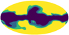 |
Fig. A.1. Raw masks used in the simulations: fsky = 0.7 (dark blue), fsky = 0.6 (light blue) and fsky = 0.5 (green). |
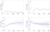 |
Fig. A.2. Best-fit values of the |


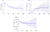 |
Fig. A.3. Best-fit values of the |


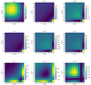 |
Fig. A.4. Two-dimensional SED shapes of the moment expansion parameters and the CMB in the (νi,νj) space for the nine LiteBIRD frequencies used throughout this work. The intensities are all expressed in MJy2 normalized by the squared SED at ν0 = 353 GHz. |
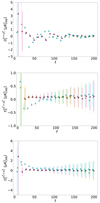 |
Fig. A.5. β − 2 moment coefficients for different fsky: fsky = 0.7 (cyan), fsky = 0.6 (purple) and fsky = 0.5 (gold). |
All Tables
Instrumental characteristics of LiteBIRD used in this study (adapted from Hazumi et al. 2020, see Sect. 3.2.3).
Best-fit values of in units of 10−4 for different values of ℓcut for the d1c simulations with fsky = 0.7, when applying the rβ-T fitting scheme.
Best-fit values of in units of 10−4 for an alternative d1c simulation with rsim = 0.01 on fsky = 0.7, and with rsim = 0 but on fsky = 0.5 and fsky = 0.6.
All Figures
|
Fig. 1. Mean value over the Nsim simulations of the B-mode angular power spectra 𝒟ℓ(νi × νj) for the d1c simulation type, with rsim = 0. The color bar spans all the Ncross spectra 𝒟ℓ(νi × νj), associated to their reduced cross-frequency |
| In the text | |
|
Fig. 2. Correlation matrix ( |
| In the text | |
|
Fig. 3. Median of the reduced χ2 in every multipole bin ℓ, for all the Nsim simulations of d0 (top, orange), d1T (middle, green) and d1 (bottom, blue), on fsky = 0.7. The reduced χ2 values are reported for the four different fitting schemes: MBB (circles), β-1 (crosses), β-T (diamonds) and β-2 (triangles). The values for the four fitting schemes are shifted from each others by ℓ = 2, in order to distinguish them. The black dashed line represents |
| In the text | |
|
Fig. 4. Top: median of the best fit values of β0(ℓ) in d0 (orange), d1T (green), and d1 (blue) for the MBB (circles). βdo is marked by the dashed black line. Bottom: same as above but with T0(ℓ), the black dashed-lines being Td0 = 20 K and Td1T = 21.9 K. |
| In the text | |
|
Fig. 5. Median of the best-fit values of |
| In the text | |
|
Fig. 6. Best-fit values of the first-order moment |
| In the text | |
|
Fig. 7. Best-fit values of the second-order |
| In the text | |
|
Fig. 8. Best-fit values of the first-order |
| In the text | |
|
Fig. 9. Top panel: posterior on |
| In the text | |
|
Fig. 10. Top panel: posterior on |
| In the text | |
|
Fig. 11. Posterior on |
| In the text | |
|
Fig. 12. Correlation matrices of the 2D-SED shapes of the CMB (BCMB(νi × νj) and dust moments |
| In the text | |
|
Fig. 13. Posterior on |
| In the text | |
|
Fig. A.1. Raw masks used in the simulations: fsky = 0.7 (dark blue), fsky = 0.6 (light blue) and fsky = 0.5 (green). |
| In the text | |
|
Fig. A.2. Best-fit values of the |
| In the text | |
|
Fig. A.3. Best-fit values of the |
| In the text | |
|
Fig. A.4. Two-dimensional SED shapes of the moment expansion parameters and the CMB in the (νi,νj) space for the nine LiteBIRD frequencies used throughout this work. The intensities are all expressed in MJy2 normalized by the squared SED at ν0 = 353 GHz. |
| In the text | |
|
Fig. A.5. β − 2 moment coefficients for different fsky: fsky = 0.7 (cyan), fsky = 0.6 (purple) and fsky = 0.5 (gold). |
| In the text | |
Current usage metrics show cumulative count of Article Views (full-text article views including HTML views, PDF and ePub downloads, according to the available data) and Abstracts Views on Vision4Press platform.
Data correspond to usage on the plateform after 2015. The current usage metrics is available 48-96 hours after online publication and is updated daily on week days.
Initial download of the metrics may take a while.