© The Authors 2025

1. Introduction

Our modern understanding of cosmology relies heavily on the precise characterisation of the cosmic microwave background (CMB) signal. The temperature anisotropies of the CMB have been accurately mapped over the whole sky, validating the canonical Λ-CDM model as the best-fit model to describe the content and evolution of our Universe (Planck Collaboration I 2020; Planck Collaboration XIII 2016). Future experiments are now focusing on the fainter polarisation signal of the CMB in order to unveil the earliest phases of our cosmic history. In particular, the standard cosmological model may require a phase of accelerated expansion – cosmic inflation – occurring in the very first fraction of a second after the primordial singularity to explain multiple observational facts about the early Universe (Brout et al. 1978; Starobinsky 1980; Guth 1981). If this event occurred, it generated a gravitational wave background bathing the primordial plasma and led to a characteristic large-scale polarisation pattern – the primordial B modes – being imprinted in the CMB (Polnarev 1985; Kamionkowski et al. 1997; Seljak & Zaldarriaga 1997). In the current leading hypothesis, the energy density at the origin of cosmic inflation has to be generated by one or multiple novel fundamental fields beyond those of the standard model of particle physics. Detection of the primordial B modes thus represents one of the most ambitious targets of modern cosmology for the next decades, but it will allow for testing of fundamental physics at energy scales beyond the reach of particle accelerators. The amplitude of the primordial B modes is quantified by the tensor-to-scalar ratio r, which is directly related to the energy scale at which inflation occurred. It is constrained by current data to satisfy r≲0.03 (95% C.L.) (Tristram et al. 2022; Galloni et al. 2023). However, contemporary and future missions will probe the value of this parameter at the 10⁻³ level in the next decades (The Simons Observatory Collaboration 2019; LiteBIRD Collaboration 2023; CMB-S4 Collaboration 2019).

In order to reach such a goal, multiple challenges have to be faced. In particular, our own Galaxy produces complex polarised signals – known as foregrounds – that contaminate the CMB and are several orders of magnitude brighter than it. Distinguishing the Galactic signal from the cosmological signal requires a delicate procedure known as component separation (Dickinson et al. 2009; Planck Collaboration V 2020). As CMB experiments become increasingly sensitive to the primordial signal, they accordingly become more sensitive to the complexity of the foregrounds (Remazeilles et al. 2016). Thus, they require refined component separation methods.

In the frequency range relevant for CMB observations, the polarised Galactic foreground signal is produced by two main sources: synchrotron emission and thermal dust signal. Synchrotron, dominating at low frequencies, is generated by light charged particles (cosmic rays) accelerating and spiralling around the lines of the Galactic magnetic field (GMF). Thermal dust, dominating at high frequencies, is the consequence of stellar light being absorbed and re-emitted by dust grains populating the interstellar medium (ISM) and rotating on themselves perpendicularly to the GMF. Local physical conditions in the ISM such as temperature, composition, density, and orientation of the GMF vary across the three dimensions of the Galaxy. This fact is supported by both observational and theoretical considerations ranging from the scale of the filaments to the scale of the whole Galaxy (Ferrière 2001; Paradis et al. 2009; Ysard et al. 2013; Jaffe et al. 2013; Schlafly et al. 2016; Planck Collaboration XI 2020; Zelko et al. 2022; Rubiño-Martín et al. 2023; Pelgrims et al. 2024; Liu et al. 2025). The variation of these physical conditions is directly traced by the light charged particles and the dust grains present in the ISM and is associated with a 3D variation of their emission properties. The spectral parameters and local polarisation orientation associated to the synchrotron and the thermal dust signals thus change over the sky. As such, any astrophysical observation presents itself as a mixture of different local signals associated with different emission conditions. Here, we refer to this phenomenon as ‘mixing’ (Chluba et al. 2017). Mixing occurs along a single line of sight in the 3D Galaxy, between lines of sight in the plane of the sky (e.g. in the instrumental beam or map pixel), and over large patches of the sky when a spherical harmonic transformation is performed.

Due to the non-linearity and geometric nature of the local polarised foreground emission, the mixing has significant and interdependent consequences on the total observed signal. First, as the sum of multiple non-linear functions gives a different function, the total (polarised) intensity will not behave as the local spectral energy distribution (SED) anymore. This phenomenon is known as ‘SED distortions (Chluba et al. 2017; Remazeilles et al. 2018; Mangilli et al. 2021). Then, as the two Stokes parameters Q and U might be distorted differently, the total polarisation angle will rotate with frequency (Tassis & Pavlidou 2015; Vacher et al. 2023b). Furthermore, mixing also has consequences for the decomposition of the foreground signal into E and B modes. To the spectral rotation of the polarisation angle corresponds a rotation of the E modes into the B modes, leading to a variation of the E/B ratio of the total signal with frequency (Vacher et al. 2023a). Finally, because of the dependence of the emission properties on the direction of an observation, it is not possible to infer a map at a given frequency based on one at another frequency using a constant scaling. Consequently, the cross-frequency angular power spectra loose some power. This last phenomenon is referred to as ‘frequency decorrelation’ (Planck Collaboration Int. XXX 2016; Pelgrims et al. 2021).

Modelling and measuring all of these effects is a priority for both CMB component separation and Galactic science. Indeed, mismodelling of these properties could have dramatic consequences on the recovery of the primordial B modes through component separation in the quest for primordial inflation (BICEP2/Keck and Planck Collaborations 2015) or in the quest for a primordial EB correlation, signature of parity violating cosmic birefringence in the early Universe¹ (Diego-Palazuelos et al. 2023). On the other hand, detecting and understanding the consequences of mixing allows one to probe the variation of the properties of the ISM in the 3D Galaxy (Pelgrims et al. 2021; Ritacco et al. 2023; McBride et al. 2023).

Moment expansion (Chluba et al. 2017) models the SED distortions arising from mixing in a minimal and well motivated way through a Taylor expansion of the SED with respect to the spectral parameters, which is a framework that was also applied to the modelling of Sunyaev-Zeldovich signals to separate and compress spectral and spatial information (Chluba et al. 2013). This approach can be generalisedd to the polarised signal in order to also model the spectral variation of the polarisation angle (Vacher et al. 2023b). The formalism was further extended at the angular power spectra level in intensity and polarisation (Mangilli et al. 2021; Vacher et al. 2023a) such that the consequences of mixing can be captured even in harmonic space. The moments thus represent a very powerful path towards performing component separation of the CMB foregrounds using minimum variance approaches (Remazeilles et al. 2021; Rotti & Chluba 2021; Adak 2021; Carones & Remazeilles 2024) or parametric fitting in pixel or harmonic space (Ichiki et al. 2019; Azzoni et al. 2021, 2023; Vacher et al. 2022; Sponseller & Kogut 2022; Minami & Ichiki 2023; Wolz et al. 2024).

In this work, we use moments for the first time to understand and build thermal dust simulations containing additional complexity arising in the third dimension from the line of sight variation of the physical conditions. While this exercise can easily be done both in intensity and in polarisation, we focus on polarisation, aiming our discussion on the impact of such complexity on the measurement of the primordial B modes. The new models will be generated as variations of the ones already provided by the PySM framework, which provides full sky simulations of the foreground signals for the CMB community (Thorne et al. 2017; Zonca et al. 2021). Our objective is twofold. First, we seek to demonstrate that the moment expansion can be used to decompose and interpret the PySM models already existing and used by the CMB community. Secondly, we aim to show that the moments provide a simple and powerful tool to inject any desired additional complexity into these models. This last point is of particular interest to the study of the limits of various component separation methods.

In Sect. 2, we give a general presentation of the moment expansion formalism and its ability to model and tackle foreground complexity. In Sect. 3, we quantitatively assess such an ability by reproducing the line of sight complexity of a dust model used by the CMB community through moment expansion. In Sect. 4, we re-use the moments computed in the previous section to create maximally complex dust models in the limit set by Planck data. We then apply basic component separation techniques to these models in order to quantify the impact of the added complexity. We further attempt to interpret this impact in regard to the moment maps contained in the models. Finally, we discuss the limits of our analysis and present our conclusions in Sect. 5.

2. Moments and the third dimension

2.1. Mixing and the moment expansion formalism

We now introduce the moment expansion framework in full generality, as a powerful tool to model complexity coming from the spatial variation of the foreground properties in polarisation. Locally, the frequency dependent linearly polarised signal emitted by an idealised point x of our Galaxy² is characterised by a canonical spectral energy distribution (SED), which can be modelled by a frequency dependent complex number ${\mathcal{P}}_{\nu }=Q_{\nu }+ßU_{\nu }$, where Q_ν and U_ν are the Stokes parameters of linear polarisation. ${\mathcal{P}}_{\nu }$ can be written as

$${\mathcal{P}}_{\nu }=\mathcal{A}{\varepsilon }_{\nu }(p),$$(1)

where ɛ_ν is a real function of the frequency called the emissivity, which characterises the SED of the signal. ɛ_ν depends on a list of N real parameters p=(p₁, p₂, …, p_N) called the spectral parameters. The modulus of ${\mathcal{P}}_{\nu }$ is called the polarised intensity. $\mathcal{A}$ is a frequency independent complex number playing the role of a complex amplitude or weight. Amplitudes are usually defined as the value of ${\mathcal{P}}_{\nu }$ evaluated at an arbitrary reference frequency ν₀ ($\mathcal{A}={\mathcal{P}}_{\nu ={\nu }_0}$). The phase of $\mathcal{A}$ divided by two, $\psi =\mathrm{Arg}(\mathcal{A})/2$ is a frequency independent angle called the polarisation angle³.

In the Galaxy, the physical conditions change when considering different points of emission associated to different spatial regions. As such, different points x will be associated with different values of the complex amplitude and the spectral parameters. When an astrophysical observation is performed, the observed signal $\langle {\mathcal{P}}_{\nu }\rangle$ will be the sum of multiple local signals contained in a considered spatial region Ω as

$$\langle {\mathcal{P}}_{\nu }\rangle ={\displaystyle {\int }_{\mathrm{\Omega }}}\mathcal{A}(x){\varepsilon }_{\nu }(p(x))\mathrm{d}x.$$(2)

Such a phenomenon is referred to as ‘(spectral) mixing’ or ‘polarised mixing’ for the special case of polarisation. Since ɛ_ν(p) is not linear in p, the modulus of the total signal $\langle {\mathcal{P}}_{\nu }\rangle$ will not scale across frequencies according to ɛ_ν anymore. We talk about ‘SED distortions’. This integral will also mix different complex weights with functions of frequencies such that the polarisation angle of the observed signal $\langle \psi \rangle =\mathrm{Arg}(\langle {\mathcal{P}}_{\nu }\rangle )/2$ will become a function of frequency. We refer to this effect as ‘spectral rotation of the polarisation angle’.

Considering any microwave sky observation, mixing can occur in three different ways: i) along the line of sight in the depth of the sky, ii) in between lines of sights inside the instrumental beam and/or the sky pixel or iii) in between lines of sights over large patches of the sky when performing a spherical harmonic transformation. The consequences of ii) and iii) will depend on the instrumental setup as well as the framework used to analyse the data⁴, while i) is some physical or intrinsic mixing that is always present at some level in the analysis. It is common to distinguish the consequences of i) and ii) by naming them respectively ‘line-of-sight’ and ‘plane of sky’ complexities. However, in practice, it is impossible to create an absolute distinction between these two effects in general and they can all be modelled using the same formalism as both i) and ii) will appear identically in Eq. (2). In this work, we attempt to avoid this confusion by remaining in the context of building a model on a pixelised sphere and by distinguishing ‘intra-pixel’ and ‘inter-pixel’ complexities to describe respectively i) and ii) at a fixed pixel resolution.

The idea of the moment expansion formalism is to model the complexity arising from mixing by making a common Taylor expansion of the SED with respect to its spectral parameters, for every emission point one averages over in Eq. (2) (Chluba et al. 2017). The total resulting SED is itself be modelled by a global Taylor-like expansion, called the ‘moment expansion’ or ‘spin-moment expansion’ for its generalisation to polarisation Vacher et al. (2023b). It takes the form⁵

$$\begin{array}{cc}\hfill \langle {\mathcal{P}}_{\nu }\rangle ={\overline{\mathcal{P}}}_{\nu }(\overline{p})\times (1& +{\displaystyle \sum _i}{\mathcal{W}}_1^{p_i}{\partial }_{p_i}{\varepsilon }_{\nu }{|}_{p=\overline{p}}\hfill \\ \hfill & +\frac{1}{2}{\displaystyle \sum _{i,j}}{\mathcal{W}}_2^{p_i{p}_j}{\partial }_{p_i}{\partial }_{p_j}{\varepsilon }_{\nu }{|}_{p=\overline{p}}+\dots ),\hfill \end{array}$$(3)

where the overall factor ${\overline{\mathcal{P}}}_{\nu }=\overline{\mathcal{A}}{\varepsilon }_{\nu }(\overline{p})$ is the canonical SED with amplitude $\overline{\mathcal{A}}={\int }_{\mathrm{\Omega }}\mathcal{A}(x)\mathrm{d}x$⁶ and pivot spectral parameters $\overline{p}=({\overline{p}}_1,{\overline{p}}_2,\dots ,{\overline{p}}_N)$ around which the expansion is done. ${\mathcal{W}}_{\alpha }^p$ are the so-called p spin-moment coefficients of order α. This name is justified as it turns out that these coefficients can be understood as the statistical moments of the spectral parameters distribution weighted by the complex amplitudes⁷ as

$${\mathcal{W}}_{\alpha }^{p_i{p}_j\cdots p_{\alpha }}=\frac{{\int }_{\mathrm{\Omega }}\mathcal{A}(x)(p_i(x)-{\overline{p}}_i)(p_j(x)-{\overline{p}}_j)\cdots ·(p_{\alpha }(x)-{\overline{p}}_{\alpha })\mathrm{d}x}{{\int }_{\mathrm{\Omega }}\mathcal{A}(x)\mathrm{d}x}.$$(4)

One can interpret the real part of the first order moment as a correction to the pivot around which the expansion is performed⁸. It is hence possible to correct the pivot values as follows:

$${\overline{p}}_i\to \overline{p}{\prime }_i={\overline{p}}_i+\mathrm{Re}\left({\mathcal{W}}_1^{p_i}\right)=\mathrm{Re}\left(\frac{{\int }_{\mathrm{\Omega }}\mathcal{A}(x)p_i(x)\mathrm{d}x}{{\int }_{\mathrm{\Omega }}\mathcal{A}(x)\mathrm{d}x}\right).$$(5)

Modelling the signal as a moment expansion using $\overline{p}{\prime }_i$ as a pivot leads to an expansion with a null real part for the first order ($\mathrm{Re}\left({\mathcal{W}}_1^{p_i}\right)=0$) and expected to converge within a minimal amount of terms. The term ${\mathcal{W}}_1^{p_i}$ thus becomes a purely imaginary number that is expected to be the largest contribution to the spectral rotation of the polarisation angle, as further discussed in Appendix C.

The addition of each of the terms in Eq. (3) is expected to model finer and finer distortions of the polarised SED⁹. The term containing ${\mathcal{W}}_{\alpha }^p$ is referred to as the term of order α and we say that the expansion is performed up to order α when it includes all the terms in Eq. (3) including the order α, while all the terms of order greater than α are assumed to be strictly zero.

The formalism to model intensity ℐ_ν is absolutely identical as the one presented above, with the weights being real numbers A instead of complex ones, such that locally ℐ_ν=AI_ν(p). Following Chluba et al. (2017), real intensity moments are noted ${\omega }_{\alpha }^p$ to distinguish them from the spin moments ${\mathcal{W}}_{\alpha }^p$.

The moment expansion allowed us to model through a set of a few coefficients the complex effects of polarised mixing induced by possibly infinite emission points associated with different spectral properties. In order to account for some complexity contained along the line of sight in the third dimension, one would have to use a set of moment coefficients in each line of sight, or equivalently in every pixel of a map. As such, the information about the complexity along the third dimension within each pixel can be fully captured by a set of maps $({\omega }_i^p,{\mathcal{W}}_i^p)$ and their associated SEDs, informing about the complexity contained both in intensity and polarisation within each pixel.

2.2. Thermal dust and modified blackbodies

In this work, we focus on the thermal dust signal, which represents the main polarised foreground for CMB experiments at high frequencies (⪆70 GHz) (Krachmalnicoff et al. 2016). In the frequency interval relevant for CMB experiments, the SED of dust grains can be accurately modelled locally in both intensity and polarisation by the modified blackbody (MBB) function

$${\mathcal{P}}_{\nu }=\mathcal{A}\frac{B_{\nu }(T)}{B_{{\nu }_0}(T)}{\left(\frac{\nu }{{\nu }_0}\right)}^{\beta },$$(6)

given by the product of a blackbody spectrum B_ν at temperature T and a power-law with spectral index β, related to the grain properties. As such, the spectral parameters of this canonical SED are p=(β, T). The signal is polarised along the shape of the grain, such that $\psi =\mathrm{Arg}(\mathcal{A})/2$ is perpendicularly aligned to the GMF, providing a powerful tracer of its structure (Planck Collaboration Int. XLIV 2016).

Due to the non-linearity of the MBB function, the total SED resulting from the mixing of multiple MBB with different spectral parameters will not be an MBB. It can, however, be accurately modelled using the moment expansion given in Eq. (3), in which the derivatives are computed with respect to both β and T. Because temperatures T commonly have large values of $\mathcal{O}(10)$, the temperature differences involved in the moments can be significantly larger than 1. As such, the expansion in T can diverge and one would prefer to perform an expansion with respect to the blackbody index $\mathcal{T}=1/T$ instead. Displaying the terms of the expansion only up to first order, the spin-moment expansion thus reads¹⁰

$$\langle {\mathcal{P}}_{\nu }\rangle ={\overline{\mathcal{P}}}_{\nu }\left(\overline{\beta },\overline{\mathcal{T}}\right)\times (1+{\mathcal{W}}_1^{\beta }ln\left(\frac{\nu }{{\nu }_0}\right)+{\mathcal{W}}_1^{\mathcal{T}}\mathrm{\Delta }{\mathrm{\Theta }}_{\nu }+\cdots ),$$(7)

where $\mathrm{\Delta }{\mathrm{\Theta }}_{\nu }={\mathrm{\Theta }}_{\nu }-{\mathrm{\Theta }}_{{\nu }_0}$ and Θ_ν is the first order derivative of B_ν with respect to $\mathcal{T}$. The term ${\overline{\mathcal{P}}}_{\nu }\left(\overline{\beta },\overline{\mathcal{T}}\right)$ is later referred to as the ‘overall MBB factor’. The exact expressions of the derivatives up to fourth order can be found for example in Vacher et al. (2023b).

3. A case study: Applying moments to dust models

3.1. Modelling the signal in each pixel

We now illustrate the power of the moment formalism both to model and understand the 3D complexity contained within a sky map. To do so, we use the foreground models available within the Python Sky Model (PySM) package¹¹ (Thorne et al. 2017; Zonca et al. 2021). PySM is a python software providing different types of data-driven full-sky simulations for the Galactic emissions. These simulations are largely used by the CMB community to apply and test component separation methods. At present, the d12 model is the only PySM dust model containing complexity in the third dimension along the line of sight. Using the terminology proposed in Sect. 2, d12 is the only PySM model with intra-pixel complexity, that is with mixing occurring in each pixel at the native resolution of N_side = 512. At this resolution, the thermal dust signal in each pixel is generated as the superposition of up to six different layers of MBB emitting components as detailed in Martínez-Solaeche et al. (2018). Each layer l is associated with its own weight ${\mathcal{A}}_l$ and spectral parameters β_l and ${\mathcal{T}}_l$. As it cannot be strictly given by an MBB, we would like to assess how well the signal of d12 can be reproduced by a moment expansion performed in each pixel i_pix. To do so, we model the signal by the expansion displayed in Eq. (7). The total complex amplitude is given by $\overline{\mathcal{A}}={\sum }_l{\mathcal{A}}_l$¹². The pivots $\overline{\beta }$ and $\overline{\mathcal{T}}$ can be obtained in every pixel i_pix by using Eq. (5)¹³:

$$\overline{\beta }(i_{\mathrm{pix}})=\mathrm{Re}\left(\frac{{\sum }_l{\mathcal{A}}_l{\beta }_l}{{\sum }_l{\mathcal{A}}_l}\right),\overline{\mathcal{T}}(i_{\mathrm{pix}})=\mathrm{Re}\left(\frac{{\sum }_l{\mathcal{A}}_l{\mathcal{T}}_l}{{\sum }_l{\mathcal{A}}_l}\right).$$(8)

As further discussed in Sect. 2, this choice of pivot leads to the cancellation of the real parts of ${\mathcal{W}}_1^{\beta }$ and ${\mathcal{W}}_1^{\mathcal{T}}$, which ensures that the overall MBB factor is the closest possible MBB function we can use to model the d12 signal in each pixel. To further clarify this statement, we considered a signal given by an exact MBB with parameters β and $\mathcal{T}$. Trying to model this signal with a moment expansion using pivots β′≠β and $\mathcal{T}\prime \ne \mathcal{T}$ would lead to a non-zero value for all the moments including the first first orders. However, it would be incorrect to interpret these moments in term of deviations of the signal from an MBB function, as they simply capture the difference between the spectral parameters of the signal and the one of the overall MBB factor used in the expansion. Using instead the adjusted pivot as done here would lead to a cancellation of all the moments, revealing that the signal is indeed a perfect MBB. Any remaining non-zero moments above first order, however, would indicate deviations of this signal that cannot be captured by an MBB function. As such, with our choice of pivot, we ensure that the moment terms model only deviation to the MBB function (i.e. polarised SED distortions and rotation of the polarisation angle with frequency). The first order moments are purely imaginary and expected to contribute significantly to the spectral rotation of the polarisation angle.

We also emphasise that we computed a value of $\overline{\beta }$ and $\overline{\mathcal{T}}$ in each pixel. As such, the 2D (inter-pixel) variability of the model is expected to be entirely contained within the overall MBB factor, while the moment coefficients grasps only the intra-pixel complexity interpreted as extra variations along the third dimension. Another valid approach would have been to consider a single value of $\overline{\beta }$ and $\overline{\mathcal{T}}$ for the whole sky. In this case, the moment coefficients would have accounted for both the 2D (inter-pixel) and the 3D (pixel) complexity indistinguishably.

The spin-moment coefficients of the equations can be computed from the layers using the discrete generalisation of Eq. (4) as

$${\mathcal{W}}_{\alpha }^{{\beta }^{\delta }{\mathcal{T}}^{\gamma }}(i_{\mathrm{pix}})=\frac{{\sum }_l{\mathcal{A}}_l({\beta }_l-\overline{\beta }(i_{\mathrm{pix}}){)}^{\delta }({\mathcal{T}}_l-\overline{\mathcal{T}}(i_{\mathrm{pix}}){)}^{\gamma }}{{\sum }_l{\mathcal{A}}_l},$$(9)

where α=δ+γ. As such, expanding up to first order, one adds to the MBB the two purely imaginary moments ${\mathcal{W}}_1^{\beta }$ and ${\mathcal{W}}_1^{\mathcal{T}}$. Up to second order, the three complex moments ${\mathcal{W}}_2^{\beta }$, ${\mathcal{W}}_2^{\mathcal{T}}$ and ${\mathcal{W}}_2^{\beta \mathcal{T}}$ are added to the expansion and the third order sees the inclusion of four new complex moment maps ${\mathcal{W}}_3^{\beta }$, ${\mathcal{W}}_3^{\mathcal{T}}$, ${\mathcal{W}}_3^{{\beta }^2\mathcal{T}}$ and ${\mathcal{W}}_3^{\beta {\mathcal{T}}^2}$ etc.

The moment maps are quantifying the complexity contained in the third dimension. As complex numbers, they can be characterised either by their real and imaginary parts or by their modulus and phase. As an illustration, the modulus and phase of ${\mathcal{W}}_2^{\beta }$ are displayed in Fig. 1. Being the second order moment, ${\mathcal{W}}_2^{\beta }$ informs us about the variance of the β distribution along each line of sight, weighted by a contribution from the distribution of the polarisation angles¹⁴. The modulus $|{\mathcal{W}}_2^{\beta }|$ can be directly compared with the variance of the β distribution contained in each pixel, on the left lower panel of Fig. B.1. From the map of $|{\mathcal{W}}_2^{\beta }|$, we understand that the intra-pixel complexity of the d12 model is distributed over the sky as a Gaussian random field with clusters of higher complexity at intermediate latitudes. We thus expect the effects of mixing to be more important in the bright regions, claim which can be verified by comparing this map with the map of the distortions of the polarised SED, which are represented on the upper left panel of Fig. C.3. On the other hand, the phase map $2\psi ({\mathcal{W}}_2^{\beta })$ probes more directly regions of high ψ complexity, which correlate with the circular variance of the ψ_l in each pixel represented on the right lower panel of Fig. B.1. Without any variations of ψ_l (i.e. of the magnetic field), this phase should be strictly zero, and the moments purely real quantities¹⁵. Intuitively, the phase of the moment maps represents the ability of the moment to capture the frequency rotation of the original signal in the complex plane. One can see the strong correlation between this phase map with the upper right panel of Fig. C.3, representing the rotation of the polarisation angle in each pixel of the d12 model. All the moment maps involved for the second order expansion are displayed in Figs. C.1 and C.2, and we comment further on their values and their interpretation in Appendix C. We also note that the moment maps thus defined probe only the inter-pixel/3D properties of the models and are independent of the inter-pixel complexity of d12 that is of its structure on the sky. This property is proven in Appendix B and can also be verified by comparing the structure of the moment maps with the structure of the d12 model at ν₀ displayed on the upper panels of Fig. B.1.

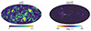Fig. 1. Maps of the modulus (left) and phase (right) of the complex spin moment ${\mathcal{W}}_2^{\beta }$ for the d12 model.

In order to evaluate the accuracy at which the moment expansion can reproduce the d12 dust model, we considered the residuals defined as

$$\frac{\mathrm{\Delta }{X}_{\alpha }}{X}=\left|\frac{X^{\text{d12}}-X_{\alpha }^{\mathrm{mom}}}{X^{\text{d12}}}\right|,$$(10)

with X∈[I, Q, U], and $X_{\alpha }^{\mathrm{mom}}$ is the value of X estimated using the moment expansion Eq. (7), including all the terms up to order α. In principle, such residuals can be computed at any frequency ν. In order to provide an illustration on a broad frequency interval relevant for CMB missions, we consider the fifteen bands of the LiteBIRD instrument between 40 and 402 GHz (LiteBIRD Collaboration 2023). The median value and median absolute deviation of the residuals are displayed in Fig. 2 for the LiteBIRD frequency range. Statistics are computed considering all the pixels on the full sky without masking and the residuals are displayed for a moment expansion performed up to different orders between zero and four. For a more quantitative estimation, the corresponding median values are reported in Table 1 for ν = 100 GHz, corresponding to a frequency band significantly different from the reference frequency (ν₀ = 353 GHz) where the dust signal is still dominant.

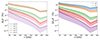Fig. 2. Residuals ΔXα/X of the spin-moment expansion for d12 expressed in percentages for the 15 bands of the LiteBIRD instrument. In the left panel is X=I, and X=Q, U is displayed in the right panel. The residuals were computed on the full sky up to a different order (α) of the expansion. The lines correspond to the median values, while the shaded areas mark the values of the median absolute deviation. We note that the blue (α = 0) and the orange (α = 1) curves are superimposed in the left panel.

One can notice clearly that the moment expansion significantly lowers the residuals by around one order of magnitude from one order to the other, thus improving the accuracy of the modelling of the intra-pixel complexity as expected¹⁶. Looking now at each individual order:

• –

  The zeroth order is given by an MBB function with a different $\overline{\beta }$ and $\overline{\mathcal{T}}$ in each pixel. With our choice of pivots, we expect this model to provide the closest possible modelling of d12 with MBB SEDs. We see that for the three states (I, Q, U), the MBB already reproduces the d12 model at the percent level, revealing that the d12 model does not inherit a lot of complexity from its third dimension. We can notice that the modelling is around two times worse for polarisation than for intensity, hinting for higher inherent complexity of the polarised signal.

• –

  The addition of the first order terms does not impact the intensity residual. This is expected as our choice of pivot values is designed to cancel any first order contribution. This is not the case for polarisation, where the imaginary contribution remains for the first order moments. The addition of this imaginary contribution drives the residuals of polarisation down to the level of the intensity ones. This reflects the fact that any polarisation angle rotation with frequency (i.e. a difference of SED between Q and U) could not be captured by the zeroth-order.

• –

  The addition of higher order terms significantly lowers the value of residuals both for intensity and polarisation. At second order of the expansion, d12 is recovered up to an accuracy of a few per ten thousand (0.01%). Pushing the expansion up to fourth order, we reach a per million (10⁻⁴%) accuracy level for the three states I, Q and U.

As such, moment coefficients clearly provide a compact and well motivated way to quantify and model any complexity (whether inter-pixel or intra-pixel) arising from mixing. Keeping all the moment contributions, one needs 2α²+4 parameters to model the signal at order α¹⁷, while one needs $4\times {\mathcal{N}}_l$ parameters to describe the sum of ${\mathcal{N}}_l$ modified blackbodies¹⁸. Thus in the present situation, we used 12 parameters at second order to model the impact of up to 24 parameters for the six layers of d12, reproducing the original signal with an accuracy of a few per ten thousands with two times less parameters. Finally, we note that the moment expansion, as a Taylor expansion, could also be able to account for more general deviation to the MBB emission-law having different origin than mixing, but this point remains to be explicitly addressed in the literature. Moreover, moment coefficients are agnostic on the number of layers and/or the specific values along the line of sight. Indeed, what is commonly modelled as discrete sums should be integrals over continuous distributions, which can then still be accurately captured with the moment expansion in an economic way.

3.2. The proxies of complexity in harmonic space

We now move into harmonic space and investigate two proxies of the complexity of the foreground signal: the decorrelation and the E/B ratio of the model. As its name suggests, decorrelation quantifies the loss of correlation between two maps at frequencies ν_i and ν_j due to mixing (Planck Collaboration Int. XXX 2016). Decorrelation can be quantified in harmonic space by the deviation from unity of the so-called spectral correlation ratio. Focusing only on the B-mode signal, it is defined as

$${\mathrm{\Delta }}_{\ell }^{\mathit{BB}}({\nu }_i\times {\nu }_j)=\frac{{\mathcal{C}}_{\ell }^{\mathit{BB}}({\nu }_i\times {\nu }_j)}{\sqrt{{\mathcal{C}}_{\ell }^{\mathit{BB}}({\nu }_i\times {\nu }_i){\mathcal{C}}_{\ell }^{\mathit{BB}}({\nu }_j\times {\nu }_j)}}.$$(11)

Another proxy of complexity is given by the frequency dependence of the E/B ratio, which is a consequence of mixing directly related to the co-variation of polarisation angles and spectral parameters¹⁹. We chose to look at the frequency dependence of the quantity

$$r_{\nu }^{E/B}=\frac{\langle {\mathcal{C}}_{\ell }^{\mathit{EE}}{\rangle }_{\ell }}{\langle {\mathcal{C}}_{\ell }^{\mathit{BB}}{\rangle }_{\ell }}(\nu ),$$(12)

where the average 〈…〉_ℓ is done over all multipole ℓ-bins considered in the analysis.

Next, we intend to compare these two quantities for the maps of d12 and its moment expansion at different orders. To do so, we use the Planck Galactic mask²⁰ with f_sky = 70% apodised with a 5° degree scale. All maps are computed with a resolution of N_side = 512 and at the four highest frequency bands of Planck, ν=[100, 143, 217, 353] GHz. Angular power-spectra are computed using NAMASTER²¹ with the B-modes purification (Alonso et al. 2019). All band-powers are binned 10 by 10 from ℓ = 2 up to ℓ = 2N_side+1.

The results can be found in Fig. 3. We observed that the expansion performed up to the second order allow both proxies to be modelled with an extremely high accuracy. The first order expansion almost enables the gap of decorrelation coming from the third dimension to be fully filled, while the expansion has to be performed up to the second order to catch the variations of $r_{\nu }^{E/B}$. As illustrated in Appendix C, this last fact can be understood by looking at the difference between the EE and the BB spectra of the moment maps, which is large when computed for the maps of ${\mathcal{W}}_2^{\beta }$. This illustration shows how powerful the moment maps can be at quantifying and modelling the complexity of a dust model within a few sets of interpretable coefficients. In theory, any foreground model, whether dust or synchrotron, can be fully represented by a set of moment maps²². Regarding both proxies and comparing d12 with the MBB case (α = 0), for which the signal is given by ${\overline{\mathcal{P}}}_{\nu }\left(\overline{\beta },\overline{\mathcal{T}}\right)$ without moments, we see that the overall MBB factor – capturing all the information about the inter-pixel complexity – represents the biggest contribution to the decorrelation and the E/B ratio variation of d12. We can thus conclude that d12 is indeed relatively complex, but that this complexity arises mostly from the spatial variation of the emission properties in 2D (inter-pixel) and not so much from variations within the third dimension (intra-pixel). From this result, one can thus wonder how much complexity can be injected in the third dimension of a model while remaining compatible with data and what could be the impact of such a complexity.

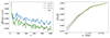Fig. 3. Two proxies of the dust complexity: decorrelation ${\mathrm{\Delta }}_{\ell }^{\mathit{BB}}(353\times 217)$ (left) and the E-to-B ratio rE/B (right). Values are plotted for the d12 original map (black crosses) and its representation by a pivot modified blackbody (blue), a moment expansion up to first order (orange) and up to second order (green).

4. Exploring alternative models for the complexity in the third dimension using moments

Next, we use the moments and their ability to model complexity in order to build new simulations of the dust emission. Our goal is to mimic mixing occurring along the line of sight with the addition of intra-pixel complexity with a set of moment maps. Obviously, the most reasonable way to proceed would be to infer this information from observational data. Unfortunately, such a complete set of information would require accurate 3D mapping of the full sky values of β, $\mathcal{T}$, I, Q, U²³, which is not yet available (some works in that direction have been undertaken recently: a map of the temperature on 3π can be found in Zelko et al. 2022 and a portion of the magnetic field has been mapped by Pelgrims et al. 2024).

While we currently lack such observationally driven moment maps over the full sky, we can investigate the impact of any arbitrary moment map introducing some additional complexity in the third dimension. In particular, we can assess the impact of the addition of moments on various observables, as the value of the angular power spectra or the decorrelation, and infer from these observables the maximal amplitude of the moments allowed by the current limit set by the measurements of the Planck mission. A simple way to move forward in this direction is to re-use the set of moment maps we already have at hand from the d12 analysis and re-inject them in a simpler model. By multiplying the moment templates by constant factors, we will be able to assess their impact on different observables and fine-tune a model containing the maximal amount of complexity with regard to limits set by current data. The goal is then to see if and how this additional 3D complexity impacts component separation for future CMB missions. As further discussed in Appendix C, we can strongly doubt that the d12 moments faithfully describe the dust complexity along the third dimension/line of sight. Specifically, they do not account for the non-Gaussian properties of the ISM. Nevertheless, the fact that they were extracted from some credible realisations of a distribution of β and $\mathcal{T}$ suggests the absence of any too pathological behaviour.²⁴ They thus provide a reasonable playground to investigate the addition of complexity at the pixel level.

As most of the complexity of d12 is arising from variations of the spectral parameters in the plane of the sky (inter-pixel mixing), we suggest to consider instead the milder PySM d10 model as our baseline. This model, based on a refined GNILC analysis of the Planck data (Planck Collaboration Int. XLVIII 2016; Planck Collaboration XII 2020) is commonly considered as a reasonable reference by the CMB community (Wolz et al. 2024; Ade et al. 2025). On the other hand, the maps of layers of β and $\mathcal{T}$ of d12 were constructed as Gaussian random realisations around the best fit values obtained in Planck Collaboration Int. XVII (2014). Contrarily to d12 d10 assumes a perfect MBB scaling in every pixel of the sky (at N_side = 512 resolution) thus containing only inter-pixel complexity arising from the variation of both β and $\mathcal{T}$. We intend to inject further complexity in each pixel using d12's moment maps and quantify the impact of such addition. As discussed in Appendix B, thanks to our choice of normalisation and pivot for the moments, the d12 moment maps contain only information about the variations along the line-of-sight but are completely agnostic on the specific values of the pivot $\overline{p}$ and amplitude $\mathcal{A}$ of d12. As such, they can be applied to any other map without introducing additional spurious and unwanted complexity from the inter-pixel properties of d12.

To simplify our discussion, we limit ourselves to the inclusion of moment contributions up to second order as we found in the previous section that this was enough to reproduce the signal of the model with an accuracy reaching the one in ten thousand level as well as the two harmonic proxies of complexity $r_{\ell }^{E/B}$ and ${\mathrm{\Delta }}_{\ell }^{\mathit{BB}}$.

4.1. Model building

We propose to create models including complexity both in the plane of the sky (inter-pixel level) and along the line of sight (intra-pixel level) using Eq. (7). The inter-pixel complexity is contained within the sky varying modified blackbody ${\overline{\mathcal{P}}}_{\nu }\left(\overline{\beta },\overline{\mathcal{T}}\right)$ of d10, where $\overline{\beta }(i_{\mathrm{pix}})$ and $\overline{\mathcal{T}}(i_{\mathrm{pix}})$ are maps containing variations over the sky. The intra-pixel complexity on the other hand will be given by the moment maps ${\mathcal{W}}_{\alpha }^p(i_{\mathrm{pix}})$ derived from the intra-pixel complexity of the d12 model.

We consider the three following models:

• –

  Model A: We first consider the model given by d10 to which complexity is added using exactly the d12 moments through Eq. (7) up to second order in each N_side = 512 native pixel. This model is expected to be less complex than d12 as it does not inherit from its 2D-complexity and thus contains less inter-pixel mixing, but it will surely be more complex than d10 due to the addition of intra-pixel complexity with the moments.

• –

  Model B: To build this model, we start from model A and multiply all the moment maps by a unique constant factor. Doing so is equivalent to rigidly amplify all the statistical moments (except the mean) of the distributions of β and $\mathcal{T}$ as well as the variation of the angles along the line-of-sight.

• –

  Model C: In this case, only the imaginary part of the moments of model A are amplified by a constant factor. As detailed in Appendix C, doing so should enhance the frequency dependence of the polarisation angles. As shown in Fig. 3, the first order (which is purely imaginary) is the main driver of the decorrelation for d12. Therefore, enhancing only the imaginary part is expected to increase ${\mathrm{\Delta }}_{\ell }^{\mathit{BB}}$ significantly.

The value of the constant factor for each model (x_B = 1.8 and x_C = 3 for models B and C respectively) is chosen such that it takes the maximal value allowed by the Planck data. Each model is indeed confronted with the values of the dust angular auto-power spectra measured by the Planck mission in Sect. 4.2. Then, we look at the proxies of the complexity ${\mathrm{\Delta }}_{\ell }^{\mathit{BB}}$ and $r_{\nu }^{E/B}$ for each model in Sect. 4.3. An interpretation of the values of the proxies in terms of moment maps is also provided. Finally, in Sect. 4.4 we address the subtraction of the simulated dust emission through standard component separation pipelines to assess the impact of the added three-dimensional complexity on CMB observations.

4.2. Comparison with Planck data

We now compare the three models A, B and C with the measurements of the polarised angular power-spectra by the Planck mission. Our goal is to use the measurements and error-bars of Planck in order to set an upper limit on the complexity that can be added to the new dust models. To do so, we defined

$$\delta {\mathcal{C}}_{\ell }^{\mathit{XX}}=\frac{|{\mathcal{C}}_{\ell }^{\mathit{XX}}(\text{d10})-{\mathcal{C}}_{\ell }^{\mathit{XX}}(\mathrm{model})|}{{\sigma }_{\mathrm{Planck}}}$$(13)

as the distance of our model to d10 in units of the Planck noise σ_Planck. Here, XX∈{EE, BB} and σ_Planck is an estimation of the Planck noise computed from the standard deviation of 600 NPIPE simulations of the sky as observed by Planck (Planck Collaboration Int. LVII 2020). The details of the derivation of σ_Planck can be found in Appendix D.

In order to be conservative, we consider that a model is rejected by data if $\delta {\mathcal{C}}_{\ell }^{\mathit{XX}}>1$. The value of $\delta {\mathcal{C}}_{\ell }^{\mathit{EE}}$ and $\delta {\mathcal{C}}_{\ell }^{\mathit{BB}}$ for the three models can be found in Appendix E for the 10 cross-spectra associated to the four highest frequencies of Planck in polarisation. For ν=ν₀ = 353 GHz, we verify that $\delta {\mathcal{C}}_{\ell }^{\mathit{XX}}=0$, for all the models, which must be true by construction.

We see that model A produces a change in the angular power spectra which is well below the limit of Planck data. Model B is instead created by multiplying all the moments of the model A by a constant number x_B until $\delta {\mathcal{C}}_{\ell }^{\mathit{XX}}$ reaches the limit of $\delta {\mathcal{C}}_{\ell }^{\mathit{XX}}=1$. We find that this limit is set by $\delta {\mathcal{C}}_{\ell }^{\mathit{EE}}(143\times 217)$ to be x_B = 1.8. The model C is built by multiplication of only the imaginary part of the moments by a constant number x_C. We chose here x_C = 3 and the model does not reach the limit of $\delta {\mathcal{C}}_{\ell }^{\mathit{XX}}=1$ for any combination of Planck frequencies. However, values of x_C>3 are rejected by the limit set by Planck data on the decorrelation (left panel of Fig. 4), which be discussed in the next section.

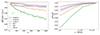Fig. 4. Comparison of the proxies of complexity, ${\mathrm{\Delta }}_{\ell }^{\mathit{BB}}$ (left) and $r_{\nu }^{E/B}$ (right), for the three proposed models (A, B, and C), d10 and d12. The black dashed lines in the left panel represent the lower limits on ${\mathrm{\Delta }}_{\ell }^{\mathit{BB}}$ set by the analysis of Planck data and taken from Planck Collaboration XI (2020).

4.3. Proxies of complexity

For all the models, we computed ${\mathrm{\Delta }}_{\ell }^{\mathit{BB}}$ and $r_{\nu }^{E/B}$ on 70% of the sky as detailed in Sect. 3. The results can be found in Fig. 4. Lower limits on ${\mathrm{\Delta }}_{\ell }^{\mathit{BB}}$ have been added in black dashed lines, taken from Planck Collaboration XI (2020) (Appendix B, Table B.1, mask ‘LR71’). We note that these limits are only available at rather large angular scales, which fortunately are also the most relevant to B-mode searches.

Regarding both proxies, the model A is only slightly more complex than d10 and less complex than d12. Such a result is expected as most of the complexity from d12 comes from the variations of its parameters on the plane of the sky as detailed in Sect. 3. However, at the smallest scales (ℓ≥500), the decorrelation of the model A becomes comparable to d12.

Model B has a larger decorrelation than d12 for ℓ≥200 and a larger $r_{\nu }^{E/B}$ for all frequencies. We thus expect this model to have either a stronger or a comparable impact than d12 on component separation and B-mode recovery.

Model C is by far the most complex model regarding both proxies. It reaches the limits of decorrelation set by Planck data for ℓ∈[11, 50] and has a greater ${\mathrm{\Delta }}_{\ell }^{\mathit{BB}}$ than d12 for ℓ≥50. Its value of $r_{\nu }^{E/B}$ is greater than d12's for all frequencies. Among the considered models, we thus expect this scenario to have the maximal impact on component separation and B-mode science.

4.4. Component separation

We now want to study the impact of the addition of pixel level complexity on component separation methods for future CMB missions. We consider a ‘LiteBIRD-like’ experiment according to the instrumental specifications reported in LiteBIRD Collaboration (2023). In order to isolate the impact of the various dust models, in this analysis we consider the simplest synchrotron model available in the literature, the PySM s0, which assumes a power-law SED with isotropic spectral index β_s across the sky and against which the two considered component separation methods have already proven to be robust. At each frequency of the data set, the foreground signal therefore includes simulated synchrotron and dust maps, with the latter varying depending on the considered model. To them, multiple realisations of CMB and instrumental noise are coadded. CMB maps are simulated through the HEALPix package (Górski et al. 2005) from the best-fit theoretical angular power spectrum of 2018 Planck data (Planck Collaboration VI 2020). Instrumental noise in each pixel is a random realisation drawn from a Gaussian distribution with standard deviation associated to the anticipated sensitivity of the corresponding frequency map (LiteBIRD Collaboration 2023). We consider the application of two component separation approaches: parametric and internal linear combination (ILC) (Bennett et al. 2003), to highlight how they can be differently affected by the complexity of the dust emission. We applied simple incarnations of the two methodologies: the multiresolution FGBuster pipeline (Stompor et al. 2009; Errard & Stompor 2019) with spectral parameters fitted in different patches across the sky and the needlet ILC (NILC, Delabrouille et al. 2009).

The FGBuster pipeline assumes a parametric model for the SEDs of the different components of the Galactic emission and fit it to the data. Specifically, best-fit values of the spectral parameters are derived by maximising the spectral likelihood defined in Stompor et al. (2009). A different value of a spectral parameter can be fitted in each pixel of an HEALPix grid with predefined resolution parameter $N_{\mathrm{side}}^{\mathrm{FGB}}$. In this analysis, we assume a power-law and an MBB as sycnhrotron and dust model, respectively. Through the FGBuster pipeline, we fit different values of the dust spectral index β, and temperature T in HEALPix patches with $N_{\mathrm{side}}^{\mathrm{FGB}}=64$ for β and $N_{\mathrm{side}}^{\mathrm{FGB}}=[8,4,0]$ for T, where the three values are associated to different regions defined by the Planck HFI masks as proposed in LiteBIRD Collaboration (2023). Only a single value is fitted for the spectral index of synchrotron β_s, as no anisotropies of synchrotron spectral properties are injected in the simulations. The NILC technique (Delabrouille et al. 2009), instead, combines data at different frequencies with frequency- and pixel-dependent weights so as to minimise locally the variance of the output map while preserving the full blackbody signal. In order to properly address the different contamination from foreground and noise, the pipeline is applied separately at different angular scales making use of the needlet filtering (Baldi et al. 2009). In this analysis, we adopt the standard needlet construction (Narcowich et al. 2006).

The outcome of component separation is assessed through the computation of angular power spectra of systematic and statistical residuals, with the former biasing the final estimate of the CMB power spectrum, while the latter contributing to its overall uncertainty²⁵. To avoid the most contaminated regions along the Galactic plane, the Planck HFI GAL70, which retains 70% of the sky, is adopted. At this stage, we focus only on the analysis of the B-mode power spectrum. Since our goal is to quantify the impact of the intra-pixel complexity on the component-separation methodologies, in Fig. 5 we display the spectral amplitude of the residuals for each model featuring 3D complexity – models A, B and C (noted respectively d10-A, d10-B, d10-C) and d12 – relatively to that obtained in the case of the analogous model but containing solely inter-pixel complexity – d10 and MBB(d12). We use the suggestive notation MBB(d12) to refer to overall MBB factor (α = 0) inferred from the d12 model in Sect. 3 (also noted ${\overline{\mathcal{P}}}_{\nu }\left(\overline{\beta },\overline{\mathcal{T}}\right)$). For completeness, the angular power spectra of the B-mode residuals after component separation are shown for both FGBuster and NILC for all the different models in Fig. E.3.

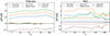Fig. 5. The ratio ${\mathcal{D}}_{\ell }^{\mathit{BB}}/{\mathcal{D}}_{\ell ,0}^{\mathit{BB}}$ compares the angular power spectra of the B-mode systematic (solid lines) and statistical (dashed lines) residuals after component separation in the case of a model with intra-pixel complexity (d10-A, d10-B, d10-C and d12) with those for their counterpart without intra-pixel complexity (d10 and MBB(d12)). Results are shown for the parametric FGBuster and blind NILC pipelines in the left and right panel, respectively. All angular power spectra are computed excluding the Galactic plane with the Planck HFI GAL70 mask which retains 70% of the sky.

Quite interestingly, the two component separation methods display very different results. The residuals for the parametric method FGBuster follow exactly the hierarchy predicted in the previous section. Indeed, models A, B, and C feature increasing amplitude of residuals accordingly to the trend of the proxies of dust complexity ${\mathrm{\Delta }}_{\ell }^{\mathit{BB}}$ and $r_{\nu }^{E/B}$ displayed in Fig. 3. Specifically, Model C, which maximises these proxies, has the largest systematic residuals at all scales, on average around 60 times greater than d10's at the spectrum level. We further observe that d12 residuals are around one order of magnitude greater than the ones of MBB(d12), implying that the additional intra-pixel complexity of d12 has a significant impact on the parametric component separation, which could not be fully anticipated by looking solely at the proxies of complexity (Fig. 3).

The NILC presents a different – if not opposite – story. Model C, expected to be the most complex according to the proxies, does not lead anymore to the highest residuals – both statistical and systematic – on the largest scales. Model B is by far the most complex, with around three times greater residuals than d10. We further note that, here again, a significant difference exists between d12 and MBB(d12).

We can attempt at interpreting these results as follows. The hierarchy of the residuals for parametric methods can be rather straightforwardly deduced from the classical proxies of foreground complexity as parametric methods are directly sensitive to the effects of mixing which introduce deviations from the canonical SED assumed in the parametric model. First, it seems that the hierarchy of the residuals for parametric methods follows the hierarchy of the classical proxies of foreground complexity (the decorrelation and the E/B ratio). This fact can be explained as parametric methods are directly sensitive to deviations from the canonical SED which they assume to model the foreground signal. Such deviations are a direct consequence of the mixing (through both the SED distortions and the spectral rotation of the polarisation angle) and are probed directly by the proxies of complexity. As discussed in Sect. 3, the imaginary part of the moments, despite having small amplitudes, can generate a pernicious complexity by entangling Q and U as well as E and B, explaining why the model C, with the largest imaginary moments, has both the largest proxies of complexity and the highest residuals for the parametric approach.

On the other hand, in regard of Fig. 5, we should conclude that minimum variance methods are not overall strongly sensitive to the effects probed by the proxies of complexities. This can be justified as the application of such methods only requires the computation of the input multifrequency covariance. Therefore, any significant foreground distortion term contributing to the covariance structure is properly addressed. Similarly, some E−B leakage and rotation of the polarisation angle is expected to have a smaller impact as these methods perform their analysis only on B-mode maps. However, we find instead that the NILC residuals correlate with the ‘relative-power’ ${\mathcal{C}}_{\ell }^{\mathit{BB}}(100)/{\mathcal{C}}_{\ell }^{\mathit{BB}}(353)$, displayed in Fig. E.4. By definition, this observable quantifies how much power is added by the moments at the frequency ν = 100 GHz, away from the reference frequency ν₀ = 353 GHz where the moment contribution is null. More precisely, the relative power is driven by the modulus of the moment maps, whose main contribution comes from their real parts, which are significantly larger in amplitude than their imaginary parts (see Appendix C). Therefore, model B, for which the moments are rigidly amplified by a constant factor, turns out to have the largest moment modulus and thus the largest relative power, and it turns out to be the most complex for NILC. We can then speculate that relative power provides a reliable proxy to assess the complexity of models regarding to NILC. We note that if such a claim revealed to be correct, it would explain a posteriori why the relative power provides such a powerful proxy in order to proceed to build clusters in advanced versions of NILC as MCNILC (Carones et al. 2023).

We note that the excursion of the residuals when some 3D complexity is injected is much higher for parametric methods ($\mathcal{O}(10)$) compared to the ones of minimum variance ($\mathcal{O}(1)$). This difference can be tentatively explained by the fact that parametric methods perform very efficiently when the parametric model is close to the data signal (d10, MBB(d12)) while their performance is greatly degraded when the signal deviates strongly from the assumed SED model. 3D complexity thus represent a major challenge for these methods as it introduces such deviations in each pixel (as in the cases of d12, d10-A, d10-B and d10-C). On the other hand, minimum variance approaches do not assume a model, and therefore, their performance does not depend on the origin of the complexity, that is, whether the complexity arises from 2D (inter-pixel) or 3D (intra-pixel) distortions. Nevertheless, all the previously discussed results aim only at investigating the hierarchy of the impact of the different models after application of component separation. We are not assessing here the general capability of component separation to deal with the most complex models. A more careful application of FGBuster as the one proposed in Puglisi et al. (2022), alternative parametric methods based on moments (Ichiki et al. 2019; Azzoni et al. 2021; Vacher et al. 2022) or minimally informed (Leloup et al. 2023; Morshed et al. 2024), as well as extended versions of NILC as MC-NILC or oc-MILC (Remazeilles et al. 2021; Carones et al. 2024; Carones & Remazeilles 2024) might be able to provide an effective reconstruction of the CMB signal for such challenging models including intra-pixel complexity. For the same reason, we do not take some realistic effects into account in the simulations, such as the scanning strategy or instrumental systematics, despite the latter have been shown to be deeply coupled with the background foreground model (Planck Collaboration Int. LVII 2020; Delouis et al. 2019; Watts et al. 2023). Still, we conclude that special care has to be given on attempts at assessing the complexity of a foreground model since such a question is deeply dependent on the component separation method under consideration. Different methods are sensitive to different facets of foreground complexity, and the moment coefficients provide a powerful tool to separate and study these different aspects. Still, we were able to propose novel alternative models – such as model B – which present a significant challenge for both parametric and minimum variance methods while remaining compatible with data.

We also note that the present analysis assumed simple Gaussian white noise without any additional systematic effect. A more realistic analysis would also have to deal with the complex coupling between systematic effects (calibration of the polarisation angle, far side lobe leakages, gain uncertainties…) and the additional complexity added to the foreground. In many cases, the foreground and the systematic complexity become entangled, such that it becomes an extremely difficult task to separate them.

5. Discussion and conclusion

In this work, we have demonstrated that the use of moment maps provides a powerful tool to quantify and model the complexity of the foreground SED models in a minimal and simple way. In principle, the complexity of virtually any foreground model currently used by the CMB community can be re-expressed by a set of moment maps. This complexity can then be amplified or reduced in a consistent way by changing the amplitude or patterns of these maps as desired. This approach allows one to perform careful studies of the link between the complexity contained in the maps and the impact of this complexity on the power spectra and component separation. In our analysis, we provided a first application of this concept by accurately reproducing the most complex PySM dust model (d12) in terms of moment maps. We were able to reproduce such a model at the one-per-ten-thousand level using five moment maps at the second order of the expansion. In doing so, we learned that despite their small amplitudes, the imaginary parts of the first order moments are the main drivers of B-mode decorrelation. The expansion, however, must be pushed up to the second order to accurately recover the dependence of the E/B ratio with frequency. In a second step, we re-used d12's moment maps to inject some additional complexity into each pixel of a simpler foreground model (d10), simulating the presence of mixing along the line of sight. This injection was done in a self-consistent fashion, which can be interpreted in terms of ISM physics. By scaling these moment maps, we were able to build extremely complex models with regard to the proxies of complexity given by decorrelation of the B-modes ${\mathrm{\Delta }}_{\ell }^{\mathit{BB}}$ and spectral dependence of the E-to-B ratio $r_{\nu }^{E/B}$. As such, we proved that all the models currently used by the CMB community (including d12) contain much milder distortions coming from the third dimension than what can be allowed by data. It is thus crucial to assess whether component separation methods are robust enough to handle these new complex scenarios.

Using component separation on the newly constructed models, we saw that the additional complexity could have a significant – but not insurmountable – impact on the quality of the reconstruction of CMB polarisation fields. Quite interestingly, different component separation methods are not sensitive to the same kind of complexity in the same way to the point that they do not agree on what is the most complex model. Parametric methods, such as FGBuster, are very sensitive to deviations of the signal from a canonical SED. They are thus more impacted by models having significant decorrelation and frequency dependence of the E/B ratio, which can be largely driven by the imaginary part of the first order moment maps, as discussed in Sect. 3. On the other hand, minimum variance methods are pretty much insensitive to this complexity but are more sensitive to the total power added by the moment maps to the foreground signal. They are thus sensitive to the modulus of the moment maps regardless of whether the complexity is coming from their real or imaginary part. A lesson therefore learned from this investigation is that caution is required when assessing the ‘complexity’ of a model, as the different quantifiers of this complexity can depict contradictory stories.

The models studied here must be understood as toy models that allow for the investigation of the relevance of the moment expansion formalism for foreground modelling as well as the impact of some possible additional complexity in the third dimension. However, it is clear that none of these models can pretend to be physical and representative of the actual or expected complexity of the sky. Clearly, the moment maps used in this work do not contain the non-Gaussian complex structure characteristic of the cosmic dust signal. While it has been recently suggested by Abril-Cabezas et al. (2024) that component separation for the CMB is largely insensitive to such non-Gaussianities, the impact of non-Gaussian moments has never been discussed as of yet. Powerful tools such as Minkowski functionals (Carones et al. 2024; Carrón Duque et al. 2024) and more generically scattering transforms (Allys et al. 2019; Delouis et al. 2022; Mousset et al. 2024) could be used to study and model these non-Gaussianities on the sphere. Furthermore, we established the validity of our models solely based on the differences of their polarised angular power-spectra power with the measurement of the Planck satellite. Doing so ensured that the sum of the inter-pixel complexity and the added intra-pixel complexity is statistically compatible with current data. However, a refined-map based analysis could certainly reject the existence of certain deterministic patterns injected in the models. Such an analysis, however, would be difficult to perform consistently, as the current CMB data is not sensitive enough to allow one to distinguish the inter- and the intra-pixel complexities. As such, our analysis can only claim to explore the upper limits on the total complexity of the foregrounds and its impact, and it does not build any new realistic and fine tuned models. The addition of other data than the CMB observations would be necessary to build realistic moment maps and finely distinguish the plane of sky and the line of sight contributions. In the long term, measurements such as the ones of Zelko et al. (2022) and Pelgrims et al. (2024) should be used to place refined bounds and build more realistic and reliable moment maps representing the actual complexity contained in the third dimension. Until then, one remains free to fine-tune as desired the morphologies and amplitudes of the added moment maps in order to introduce and study the effect of non-Gaussianities or any other kind of complexity.

The present analysis focused on the impact of thermal dust on the recovery of the primordial B modes. However, it would be straightforward and beneficial to apply such a methodology in other contexts. Firstly, the complexity of any type of foreground signal other than dust can be similarly interpreted, decomposed, and amplified using moment maps. A natural further step would then be to repeat the present work focusing on the synchrotron emission. Secondly, additional line-of-sight complexity must also impact at some level the recovery of the CMB EB spectra. To assess this impact, one must consider the addition of the moment spectral complexity to a model containing a significant EB foreground signal, such as the one proposed in Hervías-Caimapo et al. (2024), and see whether or not analysis similar to the ones performed in Diego-Palazuelos et al. (2023), Jost et al. (2023) remain robust in such maximally complex scenarios. Thus, more general studies providing a systematic link between different sets of moment maps and the resulting 3D complexity for various types of foregrounds and analysis are much desired and will be provided in future works.

Acknowledgments

LV would like to thank Carlo Baccigalupi for constant support, comments and useful discussions through the entirety of this project. LV and AC acknowledge partial support by the Italian Space Agency LiteBIRD Project (ASI Grants No. 2020-9-HH.0 and 2016-24-H.1-2018), as well as the RadioForegroundsPlus Project HORIZON-CL4-2023-SPACE-01, GA 101135036. MR acknowledges the support of the Spanish Ministry of Science and Innovation through projects PID2022-139223OB-C21 and PID2022-140670NA-I00, funded by the Spanish MCIN/AEI/10.13039/501100011033/FEDER, UE.

References

Appendix A: A word on normalisation

The moments coefficients can be defined using different choices of normalisations. Such a choice must be made carefully depending on the problem at stake, as divergences can appear in the case of the polarised signal. Writing explicitly the modified blackbody function, the expansion considered in this work (given by Eq. (7)) becomes

$$\langle {\mathcal{P}}_{\nu }\rangle =\overline{\mathcal{A}}{\left(\frac{\nu }{{\nu }_0}\right)}^{\overline{\beta }}{B}_{\nu }(\overline{\mathcal{T}})\times (1+{\mathcal{W}}_1^{\beta }ln\left(\frac{\nu }{{\nu }_0}\right)+{\mathcal{W}}_1^{\mathcal{T}}\mathrm{\Delta }{\mathrm{\Theta }}_{\nu }+\cdots ),$$

where in the discrete case, the auto spin moments are defined as ${\mathcal{W}}_{\alpha }^p={\sum }_i{\mathcal{A}}_l(p_l-\overline{p}{)}^{\alpha }/\mathcal{A}$ with $p\in \{\beta ,\mathcal{T}\}$ and the sum is ranging on the number of layers.

Alternatively, one can rewrite this expansion as

$$\langle {\mathcal{P}}_{\nu }\rangle ={\left(\frac{\nu }{{\nu }_0}\right)}^{\overline{\beta }}{B}_{\nu }(\overline{\mathcal{T}})\times (\overline{\mathcal{A}}+{\tilde{\mathcal{W}}}_1^{\beta }ln\left(\frac{\nu }{{\nu }_0}\right)+{\tilde{\mathcal{W}}}_1^{\mathcal{T}}\mathrm{\Delta }{\mathrm{\Theta }}_{\nu }+\cdots ),$$

renormalising the moments as ${\tilde{\mathcal{W}}}_{\alpha }^p={\sum }_i{\mathcal{A}}_l(p_l-\overline{p}{)}^{\alpha }$. This second choice of normalisation should in general be preferred as the first one can diverge in the regions where $\mathcal{A}\to 0$. Discussions on this point can be found in Vacher et al. (2023b) and Vacher et al. (2023a).

In the present work, we preferred the first choice of normalisation, as it allows the moment maps to ’forget’ about the structure of the original map contained in $\mathcal{A}$, such that they can be applied identically to any other maps. While this is clear when comparing the definitions of ${\mathcal{W}}_{\alpha }^p$ with ${\tilde{\mathcal{W}}}_{\alpha }^p$, we justify further this point in Appendix B. Furthermore, using the first choice of normalisation, moments are unitless coefficients associated with clear interpretations which are lacking using the second choice. We discuss how to provide such interpretations for the case of d12 in Appendix C.

However, our choice of normalisation can reveal problematic due to possible divergences in regions where the polarised signal is close to zero. As a sanity check, we verified that no outliers points were caused by such divergences and we reproduced our application to the d12 model presented in Sect. 3 using the second choice of normalisation, leading to identical results.

Nevertheless, we note that divergences cannot be evaded when computing the pivot, which expression does not depend on the choice of normalisation (Eq. (5)). In this work, we avoided such a problem by forcing the pivot to take the value of intensity when its value was outside of a given interval (see footnote ¹³).

Appendix B: Universality of the moment maps

We computed our moments from the d12 maps using Eq. (4) and the pivots computed with Eq. (8). When applying these moments directly to the other model d10, one can worry that doing so will carry along some inter-pixel complexity of the original map of d12 and not only information about the complexity contained within the line of sights.

To do things properly, we tried to find some other set of parameters ${\tilde{\mathcal{A}}}_l$ and ${\tilde{p}}_l$ satisfying the properties

$${\displaystyle \sum _l}{\tilde{\mathcal{A}}}_l=\overline{\mathcal{A}}(\text{d10})$$(B.1)

$$\mathrm{Re}\left(\frac{{\sum }_l{\tilde{\mathcal{A}}}_l{\tilde{p}}_l}{{\sum }_l{\tilde{\mathcal{A}}}_k}\right)=\overline{p}(\text{d10})$$(B.2)

and which could model the 3D complexity for d10 with the statistics of the layers from d12. Equation (B.1) asks that the sum of all the new amplitudes ${\tilde{\mathcal{A}}}_l$ should gives back the total amplitude of d10 instead of of d12, while the second asks that the pivot of the moment expansion should be the spectral parameters of d10 and not the ones of d12.

First, we can redefine the amplitudes in the layers as ${\tilde{\mathcal{A}}}_l=\overline{\mathcal{A}}(\text{d10}){\mathcal{A}}_l/\overline{\mathcal{A}}(\text{d12})$ which satisfies Eq. (B.1). Due to our choice of normalisation, it is clear that such a constant rescaling will have no impact on the value of the moments nor the pivots.

Then, we can redefine the parameters ${\tilde{p}}_l=p_l+\overline{p}(\text{d10})-\overline{p}$ which satisfies Eq. (B.2). Since ${\tilde{p}}_l$ are different from p_l only by a constant shift, all their statistical properties but the mean should remain unchanged, thus preserving the original intra-pixel complexity.

The values of the moments with this rescaling will then be

$${\mathcal{W}}_{\alpha }^p=\frac{{\sum }_l{\tilde{\mathcal{A}}}_l({\tilde{p}}_l-\overline{p}(\text{d10}){)}^{\alpha }}{{\sum }_l{\tilde{\mathcal{A}}}_k}$$(B.3)

$$=\frac{{\sum }_l{\mathcal{A}}_l(p_l+\overline{p}(\text{d10})-\overline{p}-\overline{p}(\text{d10}){)}^{\alpha }}{{\sum }_l{\mathcal{A}}_k}$$(B.4)

$$=\frac{{\sum }_l{\mathcal{A}}_l(p_l-\overline{p}{)}^{\alpha }}{{\sum }_l{\mathcal{A}}_k},$$(B.5)

which is nothing less than the value of the original moments computed from d12. As such, a given set of moment maps can be associated to any sky map regardless of its amplitude and spectral parameters as the moment maps contains only information about the third dimension. This last point can be verified by comparing the moment maps such as the one of Fig. 1 with some of the inter-pixel and intra pixel properties of d12 displayed in Fig. B.1. The moment maps thus normalised do not correlate with the polarised amplitude or polarisation angles of the d12 maps, but only quantify the 3D complexity contained in each pixel.

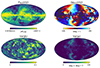Fig. B.1. Upper panels: Polarised intensity (upper left) and absolute value of the polarisation angle (upper right) of the d12 model observed at ν0 = 353 GHz. Lower panels: Variances of the spectral index βl (lower left) and (circular) variance of the polarisation angles ψl contained in each pixel of the d12 at the native resolution.

Appendix C: Interpreting d12's moment maps

All the moment maps appearing as ${\mathcal{W}}_{\alpha }^p$ in Eq. (7) are spin-2 fields on the sphere, or simply put maps of complex numbers. They quantify the complexity arising from the co-variations of the spectral parameters and the angles along the line of sight. The total map in each pixel is thus the product of ${\overline{\mathcal{P}}}_{\nu }\left(\overline{\beta },\overline{\mathcal{T}}\right)$ which is a perfect MBB map with varying $\overline{\beta }$ and $\overline{\mathcal{T}}$ in each pixel and the correction term added by the moments arising from additional complexity in the line of sight (or in 2D inside the pixel). Each moment of order α of the parameter p is related to the statistical moment of order α (mean, variance, skewness...) of the distribution of p along the line of sight.

The full sky maps of the modulus and phase of the spin moment maps present in the expansion of d12 at second order can be found in Fig. C.1, and their real and imaginary parts are displayed in Fig. C.2. The maps of the real and imaginary parts (as well as the modulus) present a Gaussian structure lacking the characteristic non-Gaussian features of the ISM. Strong similarities can be seen between the real parts and modulus of ${\mathcal{W}}_2^{\beta }$ and ${\mathcal{W}}_2^{\mathcal{T}}$, translating a strong correlation between β and $\mathcal{T}$ also visible in the non-zero value of $\mathrm{Re}({\mathcal{W}}_2^{\beta \mathcal{T}})$. The real moment maps display some 'spots’ of negative regions which might appear as pathological. These spots are associated with regions of high variations of ψ along the line of sight in which the moments can rotate and acquire a significant phase and randomly acquire a negative real component (as an Euclidian vector in a Cartesian frame pointing towards the x direction v=v_xu_x acquires general components v_x′ and v_y′ after rotation, which can be either positive or negative). These negative regions are regions where the phase of the moment maps has a high variability (Fig. C.1) and are strongly correlated with regions of large variance of ψ along the line of sight (bottom panel of Fig. B.1).

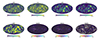Fig. C.1. Full sky maps of the modulus and phase of all the spin moments involved in the expansion of the d12 map at the second order. We note that the phase of first order moments, not represented here, are strictly equal to 90° on the whole sky, translating that they are pure imaginary numbers. They thus contribute maximally to the spectral rotation of the polarisation angles.

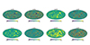Fig. C.2. Full sky maps of the real and imaginary parts of all the non-zero spin moments involved in the expansion of the d12 map at the second order.

In the case where no variation of the polarisation angles exist along the line-of-sight, the moments are purely real maps. In that case the modified blackbody map ${\overline{\mathcal{P}}}_{\nu }\left(\overline{\beta },\overline{\mathcal{T}}\right)={\overline{Q}}_{\nu }+ß{\overline{U}}_{\nu }$ is only multiplied by real functions of the frequency, modifying the SED in each pixel without any transfer of Q into U.

On the other hand, the imaginary parts of the moments result from the combined variation of large deviations of p_l from $\overline{p}$ and variation of the different polarisation angle along the line of sight ${\psi }_l=\mathrm{Arg}({\mathcal{A}}_l)/2$. Non-zero imaginary moments will unavoidably result in a transfer of $\overline{Q}$ into $\overline{U}$ inducing a greater variation of the polarisation angles with frequency for the total map along with a modification of the polarised SED.

As illustrated in Fig. C.3, the presence of the β moments are the main driver of the complexity contained within d12. The coefficient $\mathrm{Re}({\mathcal{W}}_2^{\beta })$ presents the strongest correlation with the deviation of the polarised intensity from a modified blackbody in each pixel (ΔP/P). As such, the large standard deviation of β in each pixel is the main driver of the SED distortions. The real parts of the other moments, $\mathrm{Re}({\mathcal{W}}_2^{\mathcal{T}})$ and $\mathrm{Re}({\mathcal{W}}_2^{\beta \mathcal{T}})$ also present a significant correlation with ΔP/P as well as $\mathrm{Im}({\mathcal{W}}_2^{\beta })$ and $\mathrm{Im}({\mathcal{W}}_1^{\beta })$ such that the other moment terms also contribute in a lesser extend to the value of ΔP/P.

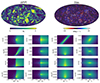Fig. C.3. Upper panels: Maps of the distortion of the polarised intensity ΔP/P (left) and the spectral rotation of the angles Δψν (right) for the d12 model. Bottom panels: Relation between the moments value in every pixel and the the two quantities presented in the upper panels. Δψν is defined as the difference of the polarisation angle in each pixel between the d12 emission at 100 and at 353 GHz. ΔP/P is defined as $(P_{\text{d12}}-\overline{P})/P_{\text{d12}}$, where Pd12 is the polarised intensity ($P=\sqrt{Q^2+U^2}$) of the original d12 model, while $\overline{P}$ the one of the pivot modified blackbody of the expansion.

On the other hand, the values of $\mathrm{Im}({\mathcal{W}}_1^{\beta })$ and $\mathrm{Im}({\mathcal{W}}_1^{\mathcal{T}})$ are strongly correlated with the variation of the total polarisation angle Δψ_ν between 100 and 353 GHz. This is no surprise as these coefficients are expected to represent the leading order terms for the spectral rotation of ψ as discussed in Vacher et al. (2023b, a). As expected from our previous discussion, the real part of the moment coefficients are not significantly correlated with Δψ_ν while the imaginary parts $\mathrm{Im}({\mathcal{W}}_2^{\beta })$ and $\mathrm{Im}({\mathcal{W}}_2^{\mathcal{T}})$ display a ‘butterfly’ shape that allows for possible correlation.

The connection between the moment maps and the proxies of complexity as ${\mathrm{\Delta }}_{\ell }^{\mathit{BB}}$ and $r_{\nu }^{E/B}$ is not as straightforward in the general case. The final impact will result from a combination of the original map and the moment angular power spectra. We note that, in the normalisation used here, even constant moment maps would have a significant impact, as each term in Eq. (7) is multiplied by the original map ${\overline{\mathcal{P}}}_{\nu }\left(\overline{\beta },\overline{\mathcal{T}}\right)$. This choice of normalisation for the moments is further justified and discussed in Appendix A.

The BB and EE angular power spectra of the d12 moment maps multiplied by $\mathcal{A}$ are displayed on Fig. C.4. They all behave as inverse power laws in ℓ, which is characteristic of foreground spectra. Here again, we see clearly that the first and second order terms in β are dominant. The difference between the E- and the B-spectra are responsible for the values of $r_{\nu }^{E/B}$. We see that this difference is larger for second order terms than the first first orders, thus explaining the results on the right panel of Fig. 3. Just like lensing, moments will mix the E- and B-components of the signal, such that some of the dust E modes will leak into the B modes.

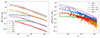Fig. C.4. Full sky angular power spectra of the moment maps of d12. All the auto-spectra of the expansion up to second order are represented on the left panel while the dominant terms of the (absolute values of the) cross-spectra on the right panel. The full lines represent the BB spectra while the dashed lines represent the EE spectra. The spectra are expressed in units of $(\mu {\mathrm{K}}_{\mathit{CMB}}{)}^2·{\mathrm{K}}^{-2{\alpha }_{\mathcal{T}}}$ where ${\alpha }_{\mathcal{T}}$ is the order of the moment with respect to $\mathcal{T}$.

The exact link between the spin-moment maps and spectra and their impact on the total dust spectra was partially discussed in Vacher et al. (2023a) and a more detailed analysis linking the moment maps to their impact on the proxies of foreground complexity in different special cases would be needed and left for future work. Such a refined analysis would be greatly beneficial for the interpretation of the results of parametric component separation method based on moments in harmonic space as Azzoni et al. (2021) and Vacher et al. (2022).

Appendix D: Derivation of Planck error bars

The Planck NPIPE (Planck Collaboration Int. LVII 2020) data release is accompanied by 600 high-fidelity Monte-Carlo simulations that include CMB, instrumental noise, foregrounds and systematics, both for full-mission and detector-set (A, B splits) maps. The complete suite of products (frequency maps, sky models, simulations, beam window functions, time streams, and auxiliary files) is available on the facilities hosted by the National Energy Research Scientific Computing Center (NERSC²⁶). We refer to the original paper for a full description and characterisation of what is included in the simulations and how they have been produced. We use the statistics of these simulations to establish an estimation of the Planck error-bars σ_Planck used in Sect. 4.2 to assess the validity of the models.

σ_Planck is derived as the scatter of the power spectra across the 600 NPIPE simulations. We now briefly describe the steps of the pipeline adopted to analyse them:

1. Simulated HFI polarised maps at ν=[100, 143, 217, 353] GHz are loaded in at their original resolution (n_side = 2048);

2. Maps are degraded to a common resolution of n_side = 512. This step is carried out in spherical harmonics space (a_ℓm) to avoid introducing artifacts in the output maps;

3. Cross-split (A×B) and cross-frequency (ν₁×ν₂) angular power spectra are estimated with the NAMASTER (Alonso et al. 2019) python package, adopting the same configuration as the one described in Sect. 3: bandpowers with constant width of Δℓ = 10 from ℓ = 2 to ℓ = 2n_side = 1024, taking into account the mode-coupling due to the adoption of the f_sky = 70% galactic mask, correcting for the impact of instrumental beams, and with B-modes purification enabled;

4. For each simulation we end up with n_freqs(n_freqs+1)/2 = 10 power spectra, six cross- and four auto-spectra. Final estimates are the average of these spectra across all 600 simulations, while the scatter σ_Planck is obtained as the standard deviation. We notice that the latter quantity is not divided by the number of simulations employed for its estimation, as one would do if interested in the error associated with the mean. Instead, we are interested in the spread of the simulations distribution because we want to define distance thresholds considering how much these simulations can scatter.

Appendix E: Power spectra figures

This appendix contains additional figures related to power spectra discussed in the main text. Figures E.1 and E.2 present $\delta {\mathcal{C}}_{\ell }^{\mathit{XX}}$ (as defined in Eq. (13)) for the three models considered and the 10 cross-frequency angular power-spectra of the Planck HFI instrument. The full residuals for the two methods (FGBuster and NILC) can be found in Fig. E.3. Finally, Fig. E.4 present the relative power BB(100)/BB(353) estimated for d10 and the three models considered.

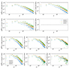Fig. E.1. $\delta {\mathcal{C}}_{\ell }^{\mathit{BB}}$, as defined in Eq. (13), for the three models and the ten cross-frequency spectra of the Planck HFI instrument.

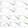Fig. E.2. $\delta {\mathcal{C}}_{\ell }^{\mathit{EE}}$, as defined in Eq. (13), for the three models and the ten cross-frequency spectra of the Planck HFI instrument.

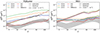Fig. E.3. Angular power spectra of B-mode residuals in the CMB solutions when using the FGBuster (left) and NILC (right) component separation methods for the different considered foreground models. Systematic residuals are shown with solid lines, while statistical ones with dashed lines. All angular power spectra are computed excluding the Galactic plane with the Planck HFI GAL70 mask which retains 70% of the sky.

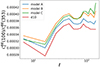Fig. E.4. Ratio of B-mode power spectrum of foreground emission at 100 and 353 GHz for d10 and the three models (A, B, and C) introduced in this work.

All Tables

All Figures

	Fig. 1. Maps of the modulus (left) and phase (right) of the complex spin moment ${\mathcal{W}}_2^{\beta }$ for the d12 model.
In the text

Fig. 2. Residuals ΔXα/X of the spin-moment expansion for d12 expressed in percentages for the 15 bands of the LiteBIRD instrument. In the left panel is X=I, and X=Q, U is displayed in the right panel. The residuals were computed on the full sky up to a different order (α) of the expansion. The lines correspond to the median values, while the shaded areas mark the values of the median absolute deviation. We note that the blue (α = 0) and the orange (α = 1) curves are superimposed in the left panel.

In the text

	Fig. 3. Two proxies of the dust complexity: decorrelation ${\mathrm{\Delta }}_{\ell }^{\mathit{BB}}(353\times 217)$ (left) and the E-to-B ratio rE/B (right). Values are plotted for the d12 original map (black crosses) and its representation by a pivot modified blackbody (blue), a moment expansion up to first order (orange) and up to second order (green).
In the text

	Fig. 4. Comparison of the proxies of complexity, ${\mathrm{\Delta }}_{\ell }^{\mathit{BB}}$ (left) and $r_{\nu }^{E/B}$ (right), for the three proposed models (A, B, and C), d10 and d12. The black dashed lines in the left panel represent the lower limits on ${\mathrm{\Delta }}_{\ell }^{\mathit{BB}}$ set by the analysis of Planck data and taken from Planck Collaboration XI (2020).
In the text

Fig. 5. The ratio ${\mathcal{D}}_{\ell }^{\mathit{BB}}/{\mathcal{D}}_{\ell ,0}^{\mathit{BB}}$ compares the angular power spectra of the B-mode systematic (solid lines) and statistical (dashed lines) residuals after component separation in the case of a model with intra-pixel complexity (d10-A, d10-B, d10-C and d12) with those for their counterpart without intra-pixel complexity (d10 and MBB(d12)). Results are shown for the parametric FGBuster and blind NILC pipelines in the left and right panel, respectively. All angular power spectra are computed excluding the Galactic plane with the Planck HFI GAL70 mask which retains 70% of the sky.

In the text

	Fig. B.1. Upper panels: Polarised intensity (upper left) and absolute value of the polarisation angle (upper right) of the d12 model observed at ν0 = 353 GHz. Lower panels: Variances of the spectral index βl (lower left) and (circular) variance of the polarisation angles ψl contained in each pixel of the d12 at the native resolution.
In the text

	Fig. C.1. Full sky maps of the modulus and phase of all the spin moments involved in the expansion of the d12 map at the second order. We note that the phase of first order moments, not represented here, are strictly equal to 90° on the whole sky, translating that they are pure imaginary numbers. They thus contribute maximally to the spectral rotation of the polarisation angles.
In the text

	Fig. C.2. Full sky maps of the real and imaginary parts of all the non-zero spin moments involved in the expansion of the d12 map at the second order.
In the text

Fig. C.3. Upper panels: Maps of the distortion of the polarised intensity ΔP/P (left) and the spectral rotation of the angles Δψν (right) for the d12 model. Bottom panels: Relation between the moments value in every pixel and the the two quantities presented in the upper panels. Δψν is defined as the difference of the polarisation angle in each pixel between the d12 emission at 100 and at 353 GHz. ΔP/P is defined as $(P_{\text{d12}}-\overline{P})/P_{\text{d12}}$, where Pd12 is the polarised intensity ($P=\sqrt{Q^2+U^2}$) of the original d12 model, while $\overline{P}$ the one of the pivot modified blackbody of the expansion.

In the text

Fig. C.4. Full sky angular power spectra of the moment maps of d12. All the auto-spectra of the expansion up to second order are represented on the left panel while the dominant terms of the (absolute values of the) cross-spectra on the right panel. The full lines represent the BB spectra while the dashed lines represent the EE spectra. The spectra are expressed in units of $(\mu {\mathrm{K}}_{\mathit{CMB}}{)}^2·{\mathrm{K}}^{-2{\alpha }_{\mathcal{T}}}$ where ${\alpha }_{\mathcal{T}}$ is the order of the moment with respect to $\mathcal{T}$.

In the text

	Fig. E.1. $\delta {\mathcal{C}}_{\ell }^{\mathit{BB}}$, as defined in Eq. (13), for the three models and the ten cross-frequency spectra of the Planck HFI instrument.
In the text

	Fig. E.2. $\delta {\mathcal{C}}_{\ell }^{\mathit{EE}}$, as defined in Eq. (13), for the three models and the ten cross-frequency spectra of the Planck HFI instrument.
In the text

Fig. E.3. Angular power spectra of B-mode residuals in the CMB solutions when using the FGBuster (left) and NILC (right) component separation methods for the different considered foreground models. Systematic residuals are shown with solid lines, while statistical ones with dashed lines. All angular power spectra are computed excluding the Galactic plane with the Planck HFI GAL70 mask which retains 70% of the sky.

In the text

	Fig. E.4. Ratio of B-mode power spectrum of foreground emission at 100 and 353 GHz for d10 and the three models (A, B, and C) introduced in this work.
In the text

References

- Abril-Cabezas, I., Hervías-Caimapo, C., von Hausegger, S., Sherwin, B. D., & Alonso, D. 2024, MNRAS, 527, 5751 [Google Scholar]
- Adak, D. 2021, MNRAS, 507, 4618 [NASA ADS] [CrossRef] [Google Scholar]
- Ade, P. A. R., Amiri, M., Benton, S. J., et al. 2025, ApJ, 978, 130 [Google Scholar]
- Allys, E., Levrier, F., Zhang, S., et al. 2019, A&A, 629, A115 [NASA ADS] [CrossRef] [EDP Sciences] [Google Scholar]
- Alonso, D., Sanchez, J., Slosar, A., & LSST Dark Energy Science Collaboration 2019, MNRAS, 484, 4127 [NASA ADS] [CrossRef] [Google Scholar]
- Azzoni, S., Abitbol, M. H., Alonso, D., et al. 2021, JCAP, 2021, 047 [CrossRef] [Google Scholar]
- Azzoni, S., Alonso, D., Abitbol, M. H., Errard, J., & Krachmalnicoff, N. 2023, JCAP, 2023, 035 [CrossRef] [Google Scholar]
- Baldi, P., Kerkyacharian, G., Marinucci, D., & Picard, D. 2009, The Annals of Statistics, 37, 1150 [Google Scholar]
- Bennett, C. L., Hill, R. S., Hinshaw, G., et al. 2003, ApJS, 148, 97 [Google Scholar]
- BICEP2/Keck and Planck Collaborations 2015, Phys. Rev. Lett., 114, 101301 [Google Scholar]
- Brout, R., Englert, F., & Gunzig, E. 1978, Annals of Physics, 115, 78 [Google Scholar]
- Carones, A., & Remazeilles, M. 2024, JCAP, 2024, 018 [CrossRef] [Google Scholar]
- Carones, A., Migliaccio, M., Puglisi, G., et al. 2023, MNRAS, 525, 3117 [Google Scholar]
- Carones, A., CarrónDuque, J., Carrón Duque, J., et al. 2024, MNRAS, 527, 756 [Google Scholar]
- Carrón Duque, J., Carones, A., Marinucci, D., Migliaccio, M., & Vittorio, N. 2024, JCAP, 2024, 039 [Google Scholar]
- Chluba, J., Switzer, E., Nelson, K., & Nagai, D. 2013, MNRAS, 430, 3054 [NASA ADS] [CrossRef] [Google Scholar]
- Chluba, J., Hill, J. C., & Abitbol, M. H. 2017, MNRAS, 472, 1195 [NASA ADS] [CrossRef] [Google Scholar]
- Clark, S. E., Kim, C. -G., Hill, J. C., & Hensley, B. S. 2021, ApJ, 919, 53 [NASA ADS] [CrossRef] [Google Scholar]
- CMB-S4 Collaboration 2019, ArXiv e-prints [arXiv:arXiv:1907.04473] [Google Scholar]
- Cukierman, A. J., Clark, S. E., & Halal, G. 2023, ApJ, 946, 106 [Google Scholar]
- Delabrouille, J., Cardoso, J. -F., Le Jeune, M., et al. 2009, A&A, 493, 835 [NASA ADS] [CrossRef] [EDP Sciences] [Google Scholar]
- Delouis, J. M., Pagano, L., Mottet, S., Puget, J. L., & Vibert, L. 2019, A&A, 629, A38 [NASA ADS] [CrossRef] [EDP Sciences] [Google Scholar]
- Delouis, J. M., Allys, E., Gauvrit, E., & Boulanger, F. 2022, A&A, 668, A122 [NASA ADS] [CrossRef] [EDP Sciences] [Google Scholar]
- Dickinson, C., Eriksen, H. K., Banday, A. J., et al. 2009, ApJ, 705, 1607 [Google Scholar]
- Diego-Palazuelos, P., Eskilt, J. R., Minami, Y., et al. 2022, Phys. Rev. Lett., 128, 091302 [NASA ADS] [CrossRef] [Google Scholar]
- Diego-Palazuelos, P., Martínez-González, E., Vielva, P., et al. 2023, JCAP, 2023, 044 [CrossRef] [Google Scholar]
- Errard, J., & Stompor, R. 2019, Phys. Rev. D, 99, 043529 [NASA ADS] [CrossRef] [Google Scholar]
- Ferrière, K. M. 2001, Reviews of Modern Physics, 73, 1031 [Google Scholar]
- Galloni, G., Bartolo, N., Matarrese, S., et al. 2023, JCAP, 2023, 062 [CrossRef] [Google Scholar]
- Guth, A. H. 1981, Phys. Rev. D, 23, 347 [Google Scholar]
- Górski, K. M., Hivon, E., Banday, A. J., et al. 2005, ApJ, 622, 759 [Google Scholar]
- Hervías-Caimapo, C., Cukierman, A. J., Diego-Palazuelos, P., Huffenberger, K. M., & Clark, S. E. 2024, Phys. Rev. D, 111, 083532 [Google Scholar]
- Ichiki, K., Kanai, H., Katayama, N., & Komatsu, E. 2019, Progress of Theoretical and Experimental Physics, 2019, 033E01 [Google Scholar]
- Jaffe, T. R., Ferrière, K. M., Banday, A. J., et al. 2013, MNRAS, 431, 683 [NASA ADS] [CrossRef] [Google Scholar]
- Jost, B., Errard, J., & Stompor, R. 2023, Phys. Rev. D, 108, 082005 [Google Scholar]
- Kamionkowski, M., Kosowsky, A., & Stebbins, A. 1997, Phys. Rev. Lett., 78, 2058 [Google Scholar]
- Krachmalnicoff, N., Baccigalupi, C., Aumont, J., Bersanelli, M., & Mennella, A. 2016, A&A, 588, A65 [NASA ADS] [CrossRef] [EDP Sciences] [Google Scholar]
- Leloup, C., Errard, J., & Stompor, R. 2023, Phys. Rev. D, 108, 123547 [Google Scholar]
- LiteBIRD Collaboration (Allys, E., et al.) 2023, Progress of Theoretical and Experimental Physics, 2023, 042F01 [Google Scholar]
- Liu, H., Li, J. -R., & Cai, Y. -F. 2025, ApJS, 276, 45 [Google Scholar]
- Mangilli, A., Aumont, J., Rotti, A., et al. 2021, A&A, 647, A52 [NASA ADS] [CrossRef] [EDP Sciences] [Google Scholar]
- Martínez-Solaeche, G., Karakci, A., & Delabrouille, J. 2018, MNRAS, 476, 1310 [Google Scholar]
- McBride, L., Bull, P., & Hensley, B. S. 2023, MNRAS, 519, 4370 [NASA ADS] [CrossRef] [Google Scholar]
- Minami, Y., & Ichiki, K. 2023, Progress of Theoretical and Experimental Physics, 2023, 033E01 [Google Scholar]
- Morshed, M., Rizzieri, A., Leloup, C., Errard, J., & Stompor, R. 2024, Phys. Rev. D, 110, 103521 [Google Scholar]
- Mousset, L., Allys, E., Price, M. A., et al. 2024, A&A, 691, A269 [NASA ADS] [CrossRef] [EDP Sciences] [Google Scholar]
- Narcowich, F. J., Petrushev, P., & Ward, J. D. 2006, SIAM Journal on Mathematical Analysis, 38, 574 [Google Scholar]
- Paradis, D., Bernard, J. P., & Mény, C. 2009, A&A, 506, 745 [NASA ADS] [CrossRef] [EDP Sciences] [Google Scholar]
- Pelgrims, V., Clark, S. E., Hensley, B. S., et al. 2021, A&A, 647, A16 [NASA ADS] [CrossRef] [EDP Sciences] [Google Scholar]
- Pelgrims, V., Mandarakas, N., Skalidis, R., et al. 2024, A&A, 684, A162 [NASA ADS] [CrossRef] [EDP Sciences] [Google Scholar]
- Planck Collaboration XIII. 2016, A&A, 594, A13 [NASA ADS] [CrossRef] [EDP Sciences] [Google Scholar]
- Planck Collaboration I. 2020, A&A, 641, A1 [NASA ADS] [CrossRef] [EDP Sciences] [Google Scholar]
- Planck Collaboration V. 2020, A&A, 641, A4 [NASA ADS] [CrossRef] [EDP Sciences] [Google Scholar]
- Planck Collaboration VI. 2020, A&A, 641, A6 [NASA ADS] [CrossRef] [EDP Sciences] [Google Scholar]
- Planck Collaboration XI. 2020, A&A, 641, A11 [NASA ADS] [CrossRef] [EDP Sciences] [Google Scholar]
- Planck Collaboration XII. 2020, A&A, 641, A12 [NASA ADS] [CrossRef] [EDP Sciences] [Google Scholar]
- Planck Collaboration Int. XVII. 2014, A&A, 566, A55 [NASA ADS] [CrossRef] [EDP Sciences] [Google Scholar]
- Planck Collaboration Int. XXX. 2016, A&A, 586, A133 [NASA ADS] [CrossRef] [EDP Sciences] [Google Scholar]
- Planck Collaboration Int. XLIV. 2016, A&A, 596, A105 [NASA ADS] [CrossRef] [EDP Sciences] [Google Scholar]
- Planck Collaboration Int. XLVIII. 2016, A&A, 596, A109 [NASA ADS] [CrossRef] [EDP Sciences] [Google Scholar]
- Planck Collaboration Int. LVII. 2020, A&A, 643, A42 [NASA ADS] [CrossRef] [EDP Sciences] [Google Scholar]
- Polnarev, A. G. 1985, Soviet Astron., 29, 607 [Google Scholar]
- Puglisi, G., Mihaylov, G., Panopoulou, G. V., et al. 2022, MNRAS, 511, 2052 [NASA ADS] [CrossRef] [Google Scholar]
- Remazeilles, M., Dickinson, C., Eriksen, H. K. K., & Wehus, I. K. 2016, MNRAS, 458, 2032 [Google Scholar]
- Remazeilles, M., Banday, A. J., Baccigalupi, C., et al. 2018, JCAP, 2018, 023 [Google Scholar]
- Remazeilles, M., Rotti, A., & Chluba, J. 2021, MNRAS, 503, 2478 [NASA ADS] [CrossRef] [Google Scholar]
- Ritacco, A., Boulanger, F., Guillet, V., et al. 2023, A&A, 670, A163 [NASA ADS] [CrossRef] [EDP Sciences] [Google Scholar]
- Rizzieri, A., Errard, J., & Stompor, R. 2025, Phys. Rev. D, 111, 043512 [Google Scholar]
- Rotti, A., & Chluba, J. 2021, MNRAS, 500, 976 [Google Scholar]
- Rubiño-Martín, J. A., Guidi, F., Génova-Santos, R. T., et al. 2023, MNRAS, 519, 3383 [NASA ADS] [CrossRef] [Google Scholar]
- Schlafly, E. F., Meisner, A. M., Stutz, A. M., et al. 2016, ApJ, 821, 78 [NASA ADS] [CrossRef] [Google Scholar]
- Seljak, U., & Zaldarriaga, M. 1997, Phys. Rev. Lett., 78, 2054 [Google Scholar]
- Sponseller, D., & Kogut, A. 2022, ApJ, 936, 8 [NASA ADS] [CrossRef] [Google Scholar]
- Starobinsky, A. A. 1980, Phys. Lett. B, 91, 99 [Google Scholar]
- Stompor, R., Leach, S., Stivoli, F., & Baccigalupi, C. 2009, MNRAS, 392, 216 [NASA ADS] [CrossRef] [Google Scholar]
- Tassis, K., & Pavlidou, V. 2015, MNRAS, 451, L90 [NASA ADS] [CrossRef] [Google Scholar]
- The Simons Observatory Collaboration 2019, BAAS, 51, 147 [NASA ADS] [Google Scholar]
- Thorne, B., Dunkley, J., Alonso, D., & Næss, S. 2017, MNRAS, 469, 2821 [Google Scholar]
- Tristram, M., Banday, A. J., Górski, K. M., et al. 2022, Phys. Rev. D, 105, 083524 [Google Scholar]
- Vacher, L., Aumont, J., Montier, L., et al. 2022, A&A, 660, A111 [NASA ADS] [CrossRef] [EDP Sciences] [Google Scholar]
- Vacher, L., Aumont, J., Boulanger, F., et al. 2023a, A&A, 672, A146 [NASA ADS] [CrossRef] [EDP Sciences] [Google Scholar]
- Vacher, L., Chluba, J., Aumont, J., Rotti, A., & Montier, L. 2023b, A&A, 669, A5 [NASA ADS] [CrossRef] [EDP Sciences] [Google Scholar]
- Watts, D. J., Basyrov, A., Eskilt, J. R., et al. 2023, A&A, 679, A143 [NASA ADS] [CrossRef] [EDP Sciences] [Google Scholar]
- Wolz, K., Azzoni, S., Hervías-Caimapo, C., et al. 2024, A&A, 686, A16 [NASA ADS] [CrossRef] [EDP Sciences] [Google Scholar]
- Ysard, N., Abergel, A., Ristorcelli, I., et al. 2013, A&A, 559, A133 [NASA ADS] [CrossRef] [EDP Sciences] [Google Scholar]
- Zelko, I. A., Finkbeiner, D. P., Lee, A., & Green, G. 2022, ArXiv e-prints [arXiv:arXiv:2211.07667] [Google Scholar]
- Zonca, A., Thorne, B., Krachmalnicoff, N., & Borrill, J. 2021, The Journal of Open Source Software, 6, 3783 [Google Scholar]