| Issue |
A&A
Volume 658, February 2022
|
|
|---|---|---|
| Article Number | A129 | |
| Number of page(s) | 22 | |
| Section | Stellar structure and evolution | |
| DOI | https://doi.org/10.1051/0004-6361/202141866 | |
| Published online | 10 February 2022 | |
Uncovering astrometric black hole binaries with massive main-sequence companions with Gaia
1
Institute of Astronomy, KU Leuven, Celestijnenlaan 200D, 3001 Leuven, Belgium
e-mail: soetkin.janssens@kuleuven.be
2
School of Physics and Astronomy, Tel Aviv University, Tel Aviv 6997801, Israel
3
Argelander-Institut für Astronomie, Universität Bonn, Auf dem Hügel 71, 53121 Bonn, Germany
4
Max-Planck-Institut für Radioastronomie, Auf dem Hügel 69, 53121 Bonn, Germany
5
Department of Particle Physics and Astrophysics, Weizmann Institute of Science, Rehovot, 7610001, Israel
Received:
23
July
2021
Accepted:
8
November
2021
Context. In the era of gravitational wave astrophysics and with the precise astrometry of billions of stellar sources, the hunt for compact objects is more alive than ever. Rarely seen massive binaries with a compact object are a crucial phase in the evolution towards compact object mergers. With the upcoming third Gaia data release (DR3), the first Gaia astrometric orbital solutions for binary sources will become available, potentially revealing many such binaries.
Aims. We investigate how many black holes (BHs) with massive main-sequence dwarf companions (OB+BH binaries) are expected to be detected as binaries in Gaia DR3 and at the end of the nominal 5-year mission. We estimate how many of those are identifiable as OB+BH binaries and discuss the distributions of the masses of both components as well as of their orbital periods. We also explore how different BH-formation scenarios affect these distributions.
Methods. We apply observational constraints to tailored models for the massive star population, which assume a direct collapse and no kick upon BH formation, to estimate the fraction of OB+BH systems that will be detected as binaries by Gaia, and consider these the fiducial results. These OB+BH systems follow a distance distribution according to that of the second Alma Luminous Star catalogue (ALS II). We use a method based on astrometric data to identify binaries with a compact object and investigate how many of the systems detected as binaries are identifiable as OB+BH binaries. Different scenarios for BH natal kicks and supernova mechanisms are explored and compared to the fiducial results.
Results. In the fiducial case we conservatively estimate that 77% of the OB+BH binaries in the ALS II will be detected as binaries in DR3, of which 89% will be unambiguously identifiable as OB+BH binaries. By the end of the nominal 5-year mission, the detected fraction will increase to 85%, of which 82% will be identifiable. The 99% confidence intervals on these fractions are of the order of a few percent. These fractions become smaller for different BH-formation scenarios.
Conclusions. Assuming direct collapse and no natal kick, we expect to find around 190 OB+BH binaries in Gaia DR3 among the sources in the ALS II, which increases the known sample of OB+BH binaries by more than a factor of 20 and covers an uncharted parameter space of long-period binaries (10 ≲ P ≲ 1000 d). Our results further show that the size and properties of the OB+BH population that is identifiable using Gaia DR3 will contain crucial observational constraints that will help us improve our understanding of BH formation. An additional ∼5 OB+BH binaries could be identified at the end of the nominal 5-year mission, which are expected to have either very short (P ≲ 10 d) or long periods (P ≳ 1000 d).
Key words: stars: black holes / binaries: general / astrometry / stars: statistics
© ESO 2022
1. Introduction
Massive stars (Minitial ≳ 8 M⊙) play an important role in the evolution of the Universe and its galaxies. Their powerful radiation fields ionise their surroundings, and their strong winds enrich the material in their neighbourhood, affecting the star formation rates and chemical compositions of their host galaxies (e.g., Heckman et al. 1990; Bresolin et al. 2008; Hopkins 2014). They typically end their lives with a powerful supernova (SN), leaving behind a compact object remnant – a black hole (BH) or a neutron star (NS). Recently, the detection of compact object mergers (e.g., LIGO Scientific Collaboration & Virgo Collaboration 2016; Abbott et al. 2016, 2017) has reignited interest in the evolution of massive stars and the formation of their remnants, as massive binaries with a BH component are a crucial phase in the evolution towards compact object mergers.
Several independent studies (e.g., Shapiro & Teukolsky 1983; van den Heuvel 1992; Brown & Bethe 1994; Timmes et al. 1996; Samland 1998) estimate that ∼108–109 stellar-mass BHs reside in our Galaxy. One way of finding these BHs is through binaries. Most massive stars are found in binaries or higher-order multiple systems and will interact with their companion during their evolution (Sana et al. 2012, 2014; Moe & Di Stefano 2017). Langer et al. (2020) predicted that ∼3% of these massive O- and early B-type stars in binaries have a BH companion, resulting in an estimated ∼1200 OB+BH systems in the Milky Way. Despite the enormous amount of predicted BHs, only 59 candidate BHs have been reported so far; all 59 have been reported in interacting binaries as X-ray sources (Corral-Santana et al. 2016), and most with low-mass, luminous companions (LCs).
Finding BHs in non-interacting binaries appears to be notoriously difficult. Two very recent examples are the BHs claimed to be present in LB1 and HR6819 (Liu et al. 2019; Rivinius et al. 2020, respectively). Soon after these claims were published, several research teams argued that these two systems did not contain BHs but were rather binaries that contain a stripped star and a Be star, or that the unseen companion is a close binary (e.g., Abdul-Masih et al. 2020; Bodensteiner et al. 2020; El-Badry & Quataert 2020; Irrgang et al. 2020; Mazeh & Faigler 2020; Shenar et al. 2020a). However, there is still an ongoing debate about the nature of these systems (Liu et al. 2020; Lennon et al. 2021). Very few other quiescent BH candidates exist in the Milky Way. Two are reported in Casares et al. (2014) and Giesers et al. (2018): a 10–16 M⊙ Be star with an orbital period of 60 days and a 0.81 M⊙ star with an orbital period of 167 days, respectively. Two more systems with giant low-mass LCs and periods below 100 days are reported in Thompson et al. (2019) and Jayasinghe et al. (2021).
The lack of BH candidates and the difficulty of showing that a BH indeed resides in those candidates (e.g., Trimble & Thorne 1969; Liu et al. 2020; Lennon et al. 2021) indicate that other methods are needed to detect these systems. The European Space Agency mission Gaia (Gaia Collaboration 2016), which is an astrometric all-sky survey, provides one such very promising method for the detection of OB+BH systems. This was already mentioned by, for example, Gould & Salim (2002) when they gave predictions on BH detections for Gaia’s predecessor HIPPARCOS. By the end of its nominal 5-year mission, Gaia will provide astrometric parameters for ∼1 billion sources brighter than G magnitude ∼20 with a precision of the order of 10–100 microarcseconds (μas). By surveying an unprecedented 1% of the stellar population in the Milky Way, Gaia will bring about a new era in the detection and analysis of the population of OB+BH binaries.
The third and most recent data release of Gaia is split into two parts, an early (EDR3) and a full data release (DR3), and is based on 34 months of observations (Gaia Collaboration 2021). Currently, only EDR3 has been published, which provided updated astrometry and photometry of ∼1.8 billion sources with a precision of the order of 0.1–1 mas (Lindegren et al. 2021). With its release, expected in the second quarter of 2022, DR3 will provide us with the first Gaia astrometric solutions of binary systems.
Several studies (e.g., Breivik et al. 2017, 2019; Mashian & Loeb 2017; Yalinewich et al. 2018; Yamaguchi et al. 2018; Wiktorowicz et al. 2019) have estimated how many binaries with a BH component Gaia will detect by the end of its nominal 5-year mission. The numbers range from hundreds to tens of thousands of systems. Identifying so few BH systems in the data of more than 1 billion sources is reminiscent of finding a few needles in a haystack. These predictions are based on the estimated precision of the data at the end of the nominal 5-year mission. However, the precision that is reached in DR3 allows for a similar analysis. With the goal of constraining massive-star evolution, in this work we focus on the massive star population (i.e. potential progenitors of BH+BH/NS).
There are multiple reasons why we could not simply scale the results obtained by previous studies. Firstly, their simulations were performed with the inclusion of initial stellar masses below 8 M⊙, whereas we only focus on the stellar population with Minitial ≳ 8 M⊙. Secondly, the simulations of Breivik et al. (2017) and Wiktorowicz et al. (2019) not only considered binaries with luminous main-sequence dwarf companions (MS+BH binaries) but also those with giant LCs, while Breivik et al. (2019) considered only the latter. Thirdly, the simulations of some previous works did not include important massive star physics. For example, Mashian & Loeb (2017) do not take into account orbital angular momentum change due to mass transfer between the components. Yamaguchi et al. (2018) neglect the wind mass loss from both stars. Binary interactions and wind mass loss are important aspects in the evolution of massive stars, the latter especially in the late stages of their evolution. Hence, these earlier simulations are not adapted to our purpose.
The goal of this paper is threefold. First, we estimate the fraction and absolute number of OB+BH systems in the second Alma Luminous Star catalogue (ALS II; Pantaleoni González et al. 2021) that will be detected as astrometric binaries in Gaia DR3 and in the data release that will come at the end of the nominal 5-year mission, DR4. The ALS II is an established catalogue of massive OB-type stars in the Gaia catalogue. While it is not complete and suffers from non-trivial selection effects (see Sect. 3.1), it is the most comprehensive catalogue of massive OB stars to date, with over 13 000 entries. In our simulations, we consider a direct collapse – all baryonic mass ends up contributing to the final BH mass – and no natal kick to be the fiducial BH-formation model. Furthermore, the predictions are based on the mass-magnitude relation for main-sequence dwarf OB stars (see Sect. 4.1). Secondly, we investigate how many of the detectable systems can be unambiguously identified as OB+BH systems. Finally, we look at the expected observable distributions of the masses of both components and the orbital period of the binary systems while also exploring the effect of different BH-formation scenarios on these distributions.
Section 2 presents the binary population synthesis simulations on which we rely. Section 3 shows the distribution of the simulated OB+BH systems according to the ALS II and explains the observational constraints imposed on their detection. We explain how we will identify the Gaia OB+BH systems in Sect. 4. The detection and identification fractions are presented in Sect. 5, together with the expected distributions of the masses and the period. We discuss our results and their uncertainties in Sect. 6 and end with a summary in Sect. 7.
2. Binary evolution models
2.1. General framework
The present work relies on the computations of Langer et al. (2020), who performed binary simulations with the stellar evolution code MESA (Modules for Experiments in Stellar Astrophysics; Paxton et al. 2011). Their simulations are tailored for massive stars and use the observed distribution of initial conditions for massive stars as determined by Sana et al. (2012):
Here, Pi is the initial period and qi is the initial mass ratio, which is the initial mass of the secondary (least massive) divided by that of the primary (most massive) star. It is the primary star that will evolve into the BH. The mass of the primary follows the Salpeter (1955) initial mass function, ranging from 10 to 40 M⊙, where the upper mass limit comes from the assumption that more massive stars undergo large inflation during their main-sequence evolution (Brott et al. 2011), inducing a common-envelope phase that leads to the merger of the binary components before the evolution towards an OB+BH system. Initial mass ratios range from 0.25 to 0.975 and orbital periods from 1.41 to 3160 days, focusing on the OB+BH population originating from post-mass-transfer binaries. The simulated systems with the longest periods evolve into a common-envelope phase, where it is assumed a merger follows before the core collapse of the primary.
For main-sequence stars that have not yet interacted, the most massive star is also the most luminous. Hence, the above-stated way of defining the mass ratio is equal to the photometric mass ratio, which is the mass of the least luminous companion (secondary) divided by that of the most luminous (primary). For the remainder of this work, we work with the photometric mass ratio, primary, and secondary.
Most of the OB+BH progenitors undergo a phase of mass transfer, after which the donor star (the BH progenitor) becomes a stripped star. Given the mass range of BH progenitors, the stripped star is expected to be a Wolf-Rayet (WR) star – a He-burning star exhibiting powerful stellar winds (Shenar et al. 2020b). Eventually, a massive enough WR star will collapse into a BH, leaving behind an OB+BH system. In their models, Langer et al. (2020) assume stars with a He-core mass MHec > 6.6 M⊙ at core carbon exhaustion become BHs through a direct collapse, meaning that all baryonic mass ends up contributing to the BH and no mass is lost through neutrinos either. Moreover, no natal kick is assumed. Stars with MHec ≤ 6.6 M⊙ are not considered BH progenitors.
The simulations of Langer et al. (2020) were, however, performed with a metallicity representative of the Large Magellanic Cloud (LMC; i.e. about half solar). If we want to obtain the same set of systems in the Milky Way, one of the major differences would be the increase in mass lost through winds, as the winds of massive stars become stronger in higher-metallicity environments (e.g., Vink et al. 2001; Crowther & Hadfield 2006; Mokiem et al. 2007). One of the downsides in using detailed model evolution codes, such as MESA, is that it requires a large amount of time and computing power to run a grid of models, such as those of Langer et al. (2020), and that uncertain parameters, such as the BH-formation mechanism, cannot easily be varied. Therefore, we worked with their original simulations for the LMC and applied a correction to the final OB+BH systems to account for first-order effects due to the transition to solar metallicity. We explore the impact of different BH-mechanisms in Sect. 6.2.
2.2. Corrections for the Milky Way
We performed two adjustments for the transformation of the systems. First, for a given stellar mass, we accounted for a temperature decrease of 1000 K (Sabín-Sanjulián et al. 2017) for the LC, hence also decreasing its luminosity through Stefan-Boltzmann’s law. The radius of the LC was unaltered. While some change in the radius is expected at different metallicity, the impact of this change is negligible. Moreover, the change in luminosity from the effective temperature is small and does not significantly alter the results presented in this work.
Second, we accounted for metallicity-dependent wind strength. Due to stronger winds in higher-metallicity environments, such as the Milky Way, the final masses of the BHs and the LCs will be lower than those in low-metallicity environments, such as the LMC. The extra mass loss also leads to an increase in period.
We used a power-law dependence of mass loss and metallicity Ṁ ∝ Z0.83, as determined by Mokiem et al. (2007). In general, the wind mass loss of WR stars obeys a slightly steeper metallicity dependence (e.g., Hainich et al. 2015), which also varies for different hydrogen surface abundances. For simplicity and to neglect scatter on the metallicity dependence, we used Ṁ ∝ Z0.83 also for the WR stars.
Since the difference in mass-loss rates of main-sequence stars is negligible, we only applied the mass-loss correction to the systems when mass transfer has fully stopped when the components detach. We used log R/log RRL < 0.99 as the criterion for detachment, where R is the radius of the primary star (the BH progenitor) and RRL is its Roche-lobe radius.
The wind mass-loss rate for the LMC was determined through ṀLMC = (Mrl−end − Mf)/Δτf,rl−end, where Δτf, rl − end is the time difference between the SN of the primary and the detachment. Through the mass-loss–metallicity relation, the mass-loss rate in the Milky Way is related to that of the LMC as

with ZMW/ZLMC = 2. The final mass of a star in the Milky Way is then given by

This correction was done for both components, where the final mass of the LC is its mass at primary BH formation.
The final period of the system due to mass loss of both components is obtained from (see Appendix A)
where the subscript ‘i’ indicates the initial conditions, in this case the conditions at detachment, and the subscript ‘f’ indicates the final conditions of the system or the conditions right before BH formation. There are a few systems that do not undergo a phase of mass transfer due to their long periods. For those systems, the initial conditions are those at the beginning of the simulations.
For the original simulations (no mass or period corrections), systems that undergo mass transfer already show a slight difference between the final period in the simulation and the period obtained with Eq. (4). One of the assumptions made when using Eq. (4) is that both stars reside well within their Roche lobe. At detachment this assumption is not valid and hence Eq. (4) might be too simplistic. Especially for short-period systems and stars close to filling their Roche lobe, tides affect the period change. Assuming tidal effects are metallicity independent, we applied a relative period change – the ratio of the period in the original system Psim, LMC and its period calculated with Eq. (4) Peq, LMC – to the final period derived with the masses in the Milky Way, such that the final period for the Milky Way systems obtained with Eq. (4) was multiplied by a factor of Psim, LMC/Peq, LMC.
The applied wind-mass-loss corrections do not lead to major changes in the distributions of the LC mass, the mass ratio, or the period post-SN between LMC and Milky Way systems, whereas the most massive BHs have slightly shifted towards lower masses. Since Ṁ increases with increasing M, the amplification of Ṁ causes the most massive BH progenitors to be over-proportionally lighter. The different distributions are shown in Appendix B.
3. The detectability of OB+BH systems with Gaia
We wish to estimate how many of the OB+BH systems that are observed by Gaia will also be detected as binaries in DR3 and in DR4. For this, we applied several observational constraints to the simulated OB+BH systems. Observational constraints are determined by the apparent G-band magnitude, which depends on the distance to the system, the period of the system, and the observed astrometric signal. A discussion on the observational constraints is given at the end of Sect. 6.1.
3.1. The distance distribution of the systems
The distance distribution of the simulated systems was based on the distances of known massive stars, and hence does not represent the intrinsic distribution in the Milky Way, but an observational one. A well-known massive star catalogue is the Alma Luminous Star (ALS; Reed 2005) catalogue. Pantaleoni González et al. (2021) have created the ALS II, in which they obtained distances for the stars in the ALS based on Gaia DR2 data and a prior tailored for massive stars. We only used the distances of sources (the number of sources is only used later in Sect. 6.1) that have high-quality DR2 data and excluded those flagged as non-massive stars. An observational constraint on the distance is embedded in the magnitude limit. The distance distribution is shown in the left panel of Fig. 1.
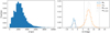 |
Fig. 1. Distances of the massive OB stars in the ALS II (left), and absolute (open blue) and apparent (open orange) magnitudes of the full sample of simulated OB+BH systems (right). The right panel also shows the absolute and apparent magnitudes of the massive stars in the ALS II (dashed black and grey, respectively). |
We note that the ALS II is not necessarily complete, but rather represents a clean sample of massive OB stars formed by compiling previous catalogues and literature sources of massive OB stars. However, for the purpose of this research, we do not require a complete sample, but instead a large and clean enough sample of known massive stars. Also, the possible lack of young massive stars (Holgado et al. 2020) is not a real concern in this research as most of the BHs are expected to have companions older than ∼5 Myr.
Since we are using a known massive star catalogue, the reported fractions strictly apply to the targets in the ALS II, and not to the full population of OB+BH systems in the Milky Way. As the true distance distribution is more skewed towards larger distances, many more systems would be too faint to be detected and hence the detection fraction would be lower.
3.2. Apparent G-band magnitudes
For reliable Gaia astrometric solutions, we applied a conservative magnitude limit of 6 < G < 20 based on EDR3 data and performance (Lindegren et al. 2021). We determined the apparent G-band magnitudes, mG, of the LCs in the OB+BH systems as

where MG is the absolute G magnitude, d is the distance to the system in parsec, and AG is the extinction in the G band per kpc. The true situation of extinction is complex and depends not only on distance, but also on position in the sky. For the simplified approach, however, an average constant extinction can be used. Using Table 3 from Wang & Chen (2019) and an average V-band extinction AV = 1 mag kpc−1 for the Milky Way (see Spitzer 1978), we obtain AG = 0.789 mag kpc−1.
We determined the absolute G-band magnitude as the difference between the bolometric magnitude and the bolometric correction factor for the G-band, or MG = Mbol − BCG. The bolometric magnitude was calculated as Mbol = −2.5log(L/L⊙)+Mbol, ⊙, where we adopted a solar value Mbol, ⊙ of 4.74. The luminosity L of an LC is determined from Stefan-Boltzmann’s law. We used the bolometric correction factors available on the MIST website1 (MESA Isochrones and Stellar Tracks; Choi et al. 2016; Dotter 2016). The correct bolometric correction factor is determined by the effective temperature and the surface gravity (g = GM/R2).
The obtained absolute and apparent magnitudes of the simulated OB+BH systems (see Sect. 5) are shown in the right panel of Fig. 1. The apparent and absolute (calculated with Eq. (5)) magnitudes of the massive stars in the ALS II are also shown as well as the imposed magnitude limits. We did not include any correlation between mass and distance when assigning distances in Sect. 3.1. The longest distances in the ALS II most likely correspond to only the most massive stars in the catalogue. Similarly, at the shortest distances lower-mass massive stars are found. Although this has not been taken into account, the closeness of the apparent magnitudes of the simulated sample and the ALS II shows that this correlation does not impact our results significantly. If any, the impact of the slight overabundance of fainter systems in the simulation is smaller detection fractions as the Gaia precision is lower for fainter stars (see Fig. 5).
3.3. The astrometric signal
For DR3, we required a conservative upper limit on the orbital period P ≤ 3 yr, such that at least one full period is covered by the data. In an extension to DR4, the maximum allowed period is 5 yr. A lower limit is determined by the astrometric signal of the binary system, which is equal to the observed angular semi-major axis of the photo-centre motion. In order for Gaia to detect a source as a binary, we required that the observed astrometric signal is significantly larger than the Gaia astrometric precision, α ≥ (3)σG as a (conservative) criterium.
The Gaia astrometric precision is magnitude dependent. For DR3, we can use the precision measured with EDR3 data. We used for the EDR3 Gaia precision the derived along-scan variance data provided to us by A. Everall (priv. comm., based on a similar method described in Everall et al. 2021). For the precision at the end of the nominal 5-year mission, we used the estimated end-of-mission precision as described in Sect. 8.1 (Eqs. (4)–(6)) of Gaia Collaboration (2016).
We determine an expression for the astrometric signal produced by the binary system, which is related to the semi-major axis of the projected orbit α and the distance d to the system through α = α/d. In binary systems with a non-luminous component, the observed photo-centre motion is equal to the motion of the LC around the common centre of mass. Its semi-major axis in the true orbit is given by aLC = aMBH/Mtot, where a = aLC + aBH is obtained from Kepler’s third law 4π2a3 = GMtotP2. The projected orbit of the LC is then determined by the orbital parameters of orientation, i (inclination), Ω (longitude of the ascending node), and ω (argument of periastron), through the Thiele-Innes constants
![$$ \begin{aligned} \begin{aligned}&A = a_{\mathrm{LC}} \left[ \cos \Omega \cos \omega - \sin \Omega \sin \omega \cos i \right],\\&B = a_{\mathrm{LC}} \left[ \sin \Omega \cos \omega + \cos \Omega \sin \omega \cos i \right], \\&F = a_{\mathrm{LC}} \left[ -\cos \Omega \sin \omega - \sin \Omega \cos \omega \cos i \right],\\&G = a_{\mathrm{LC}} \left[ -\sin \Omega \sin \omega + \cos \Omega \cos \omega \cos i \right]. \end{aligned} \end{aligned} $$](/articles/aa/full_html/2022/02/aa41866-21/aa41866-21-eq6.gif)
For the systems, Ω and ω were uniformly randomly distributed between 0 and 2π, and cos i between −1 and 1. The projected Cartesian coordinates xproj and yproj are given by
where X = cosE − e and  , with E being the eccentric anomaly.
For eccentric systems, the semi-major axis a of the orbit, hereafter called the true semi-major axis, and the semi-major axis of the projected orbit α generally do not have the same length. An example is shown in Fig. 2. For this eccentric system (see figure caption for more details), the projection of the true semi-major axis has a length of 0.75 au, while the semi-major axis of the projected orbit is αLC = 1.00 au. However, for non-eccentric systems (e = 0), we have aLC = αLC = aLC, proj, no matter the orientation of the system. (A derivation of the equality together with an expression for α for eccentric orbits is given in Appendix C).
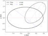 |
Fig. 2. Orbital projection for an example of a MS+BH system with MBH = 10 M⊙, MLC = 15 M⊙, aLC = 1.17 au, and e = 0.6. The solid ellipse represents the true orbit, with the semi-major axis shown as the two stars connected by a red line. The dashed ellipse shows the orbit projected with i = 60°, Ω = 52.9°, and ω = 242.4°. The projected semi-major axis is shown as a dashed red line. The blue triangles connected with a dashed line show the semi-major axis of the projected orbit, α. |
In our simulations, we used the observational constraint of α > 3σG, ignoring the orbital inclination. However, the observed astrometric signal of the orbital motion, which determines the detectability of the orbit, is the actual motion projected on the plane of the sky, and therefore depends on the orbital inclination. For inclinations larger than 0°, the projection of one of the two dimensions of the orbital motion is suppressed by cos i, and therefore the effective astrometric signal, which is used as the observational cut, is, on average, suppressed by  , a correction factor we applied in the simulations.
4. Identifying the OB+BH systems
The next step is to separate the needles – the OB+BH systems – from the haystack – normal binaries with two main-sequence components. For this, we used the method described by Shahaf et al. (2019). Their method astrometrically identifies binaries with a compact object, based on the observed astrometric signal of the binaries. Shahaf et al. (2019) define a dimensionless parameter called the astrometric mass-ratio function (AMRF, or 𝒜), defined as
where ϖ is the parallax of the system, and q = M2/M1 and S = I2/I1 are the current mass ratio and intensity ratio, respectively, of the secondary (least luminous) to the primary (most luminous) star. The intensity of a star in the G band can be defined as IG ∝ 10−0.4MG and the intensity ratio between two components hence becomes SG(M1, M2) = 10−0.4ΔMG. This expression does not take into account the age of the stars. From the mass-magnitude relation (established in Sect. 4.1) we can determine the intensity ratio for a given primary mass at different mass ratios and determine the theoretical AMRF (Sect. 4.2).
In Eq. (8), we call the expression with α the observational AMRF, or 𝒜, and the right-most expression the theoretical AMRF. As Shahaf et al. (2019) showed, the AMRF is a useful parameter for separating BH systems from non-degenerate systems, as we also show in Sect. 5.2.
4.1. The mass-magnitude relation in the G band.
Shahaf et al. (2019) have used their method on a HIPPARCOS sample of low-mass dwarf stars, establishing a piecewise linear mass-magnitude relation of the form MG = alog(M/M⊙)+b. Similarly, we derived such a logarithmic mass-magnitude relation for the GaiaG-band magnitude. Table D.1 lists the collected temperatures and radii for dwarfs with masses in between 0.20-57.95 M⊙, covering spectral types O3 V - M9 V. Using the same method as described in Sect. 3.2, we obtained the G-band magnitudes, which are shown in Fig. 3.
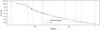 |
Fig. 3. G-band magnitudes for dwarfs in the mass range 0.2–55.67 M⊙ obtained from the literature (see Table D.1). The masses are shown on a logarithmic scale. The fit is shown with a solid red line. Grey vertical lines indicate the fitted regions. |
To establish the piecewise linear mass-magnitude relation, we divided the obtained magnitudes into different regions based on their mass. Table 1 shows the fitted regions with their respective fit parameters and the fit is shown in Fig. 3.
Fit parameters for the mass-magnitude relation of dwarfs in different mass regimes.
4.2. The theoretical AMRF curves for different masses
Shahaf et al. (2019) distinguish between different types of systems, based on the nature of the secondary star. The primary star is defined as the most massive LC (for OB+BH systems, the LC is always the primary star). Three different types of systems are defined: main-sequence binaries, triple main-sequence systems, where the secondary star is an unresolved main-sequence binary, and MS+BH binaries. For each of these cases, the same value of q will lead towards different intensity ratios S and hence Eq. (8) will appear different. We highlight that q is always defined as the mass of the companion (a BH, another main-sequence star, or a binary system) divided by the mass of the primary main-sequence star.
Figure 4 shows theoretical AMRFs obtained with the right-most term in Eq. (8), using the mass-magnitude relation derived in Sect. 4.1. We show curves for three different primary masses. The black solid line shows the theoretical AMRF for OB+BH systems. Dotted curves are for main-sequence binaries, and the dashed curves are for triple systems for which the binary companion has two equal-mass components. The triple curves are cut-off when the binary component would become brighter than the primary star.
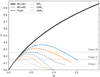 |
Fig. 4. Different theoretical AMRFs for three different primary masses: 9 M⊙ (blue), 20 M⊙ (orange), and 30 M⊙ (grey). The solid black line shows the theoretical AMRF for MS+BH systems, the dotted curves are for main-sequence binaries, and dashed curves are for triple main-sequence systems. Different classes are also indicated for the 30 M⊙ primary by the horizontal dotted lines at the maxima of the triple-AMRF and the main-sequence AMRF (Class III: identifiable OB+BH systems, Class II: triple main-sequence or OB+BH systems, Class I: OB+OB binaries, triple main-sequence systems, or OB+BH binaries). |
The dotted horizontal lines show the maximum of the theoretical AMRF for main-sequence binaries and triple main-sequence systems with a 30 M⊙ primary. Based on these maxima, Shahaf et al. (2019) distinguish between three classes (also indicated on the figure for a 30 M⊙ primary). Systems with an observational 𝒜 above the maximum of the triple-AMRF (corresponding to 0.365, 0.313, and 0.257 for the 9, 20, and 30 M⊙ primary, respectively) are classified as Class III. These system are identifiable OB+BH systems. Systems with 𝒜 above the maximum of the main-sequence AMRF (corresponding to 0.232, 0.194, and 0.156 for the 9, 20, and 30 M⊙ primary, respectively) and below the maximum of the triple-AMRF are classified as Class II. Most of these systems are triples; however, some might be OB+BH systems. Finally, Class I are those systems with an 𝒜 below the maximum of the main-sequence AMRF and hence the nature of these objects can be a main-sequence binary (most probable), a triple main-sequence system, or an OB+BH system.
Although OB+NS systems might also be present in the observed sample (i.e. in Gaia), they will most likely not be identified as Class III. For q values in the range of NS companions with massive OB-type LCs (q ∼ 0.05 − 0.3), all curves lie close to each other and hence we would not be able to distinguish between the three proposed cases.
5. The detected OB+BH distribution
To predict the theoretical distribution of the masses of the components and the orbital periods of the OB+BH systems that will be identified, we performed a statistical analysis by drawing 50 000 OB+BH systems from the simulations, using a weight factor that depends on the lifetime of the systems and the observed distributions of the initial period and masses, while assuming a constant star formation rate (see Langer et al. 2020). This way, we can estimate the fraction of OB+BH systems that can be detected and identified. Therefore, we will only report results as fractions in this section. Later, we can apply these predicted detection fractions to the expected number of identifiable OB+BH systems in the ALS II (see Sect. 6.1).
The reported fractions in this section are based on the assumption that the masses of the LCs are known. The effect of uncertainties on the masses is investigated in Sect. 6.3.
5.1. The fraction of OB+BH systems detected by Gaia
We first investigated how many OB+BH systems Gaia would be able to detect as binaries, using the observational constraints presented in Sect. 3. The results are presented in Fig. 5.
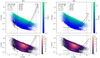 |
Fig. 5. Astrometric signal and magnitudes of the simulated OB+BH systems for DR3 (left) and for DR4 (right). The top panels are with a colour-coded period, and the bottom panels are density plots. Systems with periods longer than the upper limit of the respective data release are not shown. The vertical dotted lines in the panels show the limiting Gaia magnitude. From top to bottom, the meaning of the different entries in the legend is the fraction of OB+BH systems in total (by definition 100%), those with a G-band magnitude between 6 and 20 mag, those with a period below the upper limit, and those that have an astrometric signal larger than 1σ or 3σ, respectively. Systems that pass a certain criterion also need to have passed the criteria mentioned above it. The two higher-density regions in the bottom plot originate in the underlying period distribution related to the mass transfer event (see also the upper panel of Fig. 6 in Langer et al. 2020). Systems undergoing Case A mass transfer are found at shorter periods (the bottom region), and systems going through Case B mass transfer end up with higher periods (upper region). |
Accounting for the Gaia magnitude range, 93.1% of our simulated OB+BH binaries would be included as sources in the Gaia catalogue. Using the conservative observational limit (α > 3σ), 82.2% of those Gaia sources would be flagged as binaries in DR3, amounting to 76.5% of the entire sample. At the end of the 5-year mission, 85.0% of the entire sample will be detected as binaries. Below, we adopt these conservative detection estimates.
The lower limit imposed on the astrometric precision mostly filters out (the closest) systems with the shortest periods. Although in line with what we expect, it is worth noting that the observed population of OB+BH systems will be slightly biased towards systems with larger orbital periods. However, systems with the largest orbital periods are also excluded from detection due to the imposed upper limit on the period. Plots for the observed parameter space are shown in Fig. 6 for the masses of the components and the orbital periods as a function of the astrometric signal and corner plots of the distributions for different observable parameters are shown in Figs. E.1 and E.2 for DR3 and DR4, respectively, for the full sample, the Gaia sources, and the sources detected as binaries. The comb-like structures in the plots of the BH mass as a function of, for example, the period or astrometric signal originate in the discreteness in the initial parameters of the binary model simulation. However, Case A mass transfer – mass transfer while both components are still on the main sequence – in shorter period systems results in the fading of the discreteness in the distribution of the parameters of the post-mass-transfer systems and hence the disappearance of the comb-like structures.
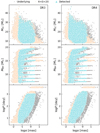 |
Fig. 6. Masses of the components and the periods as a function of the astrometric signal. The underlying distributions (those of Langer et al. 2020) are shown with black dots and overplotted with those systems having 6 < G < 20 (orange stars). On top is the subset of systems that are detected in the conservative case (i.e. α > 3σ and a period lower than the imposed upper limit; cyan triangles). The left panels are for DR3 and the right panels for DR4. The discrete BH masses come from the discrete main-sequence primary masses in the simulations of Langer et al. (2020). |
5.2. Finding the needles in the haystack: Identifying the BH+OB binaries
From the fraction of OB+BH systems that will be detected as binaries by Gaia, we investigated how many of those we can extract from the vast amount of binary sources in the Gaia binary catalogue (see Sect. 4 for the method). To only consider significant identifications, we determined if the measured value of 𝒜 − σ𝒜 of a binary system is larger than the maximum 𝒜triple reached by the triple AMRF corresponding to the mass of the LC. If this is the case, we count that system classified as an OB+BH system. We used the orbital period and the mass of the LC from the simulated systems, and their calculated astrometric signal to calculate 𝒜 (Eq. (8)) for each system. The uncertainty σ𝒜 on 𝒜 was calculated using the Gaia precision as an uncertainty on the parallax and astrometric signal, a 10% uncertainty on the period, and a 50% uncertainty on the mass.
Figure 7 shows how many of the systems classified as a binary by Gaia have 𝒜 − σ𝒜 > 𝒜triple and are hence classified as Class III systems. For DR3, 88.7% of the OB+BH systems classified as binaries are classified as Class III systems in this diagram, hereafter called the AMRF completeness. Combining this AMRF completeness with the detectable fraction, we find that we are able to identify 67.8% of all sampled OB+BH systems. For DR4, we have an AMRF completeness of 82.3%, leading to the identification of 69.9% of all sampled OB+BH systems.
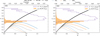 |
Fig. 7. Distribution of 𝒜 for the systems classified as a binary by Gaia. The left panel is for DR3 and the right panel for DR4. The curves are the same as in Fig. 4 (legend on top). Systems with 𝒜 − σ𝒜 > 𝒜triple (Class III) are represented by the purple open histogram, and systems with 𝒜 − σ𝒜 ≤ 𝒜triple (non-Class III) are shown with an orange filled histogram. Bins are 0.025 in width. The open histograms account for 88.7% and 82.3% of the total number of detected systems in the left and right panel, respectively. |
5.3. Distributions of the orbital period and masses
We investigated the expected distributions of the masses of the components in the identified OB+BH systems and their periods. We can determine three things: (1) the expected distributions of the systems that are observed by Gaia, (2) those of the systems that are detected as binaries by Gaia, and, more interestingly, (3) the expected distributions of the identifiable OB+BH systems. Figure 8 shows the distributions of the mass of the LC and BH, the mass ratio, and the period in DR3 and DR4.
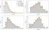 |
Fig. 8. Distribution of MLC (top left), MBH (top right), q (bottom left), and P (bottom right) in DR3 and DR4. In the legend, ‘Underlying’ is the distribution of all simulated OB+BH systems, ‘Detected’ are those systems detected as binaries by Gaia, and ‘Identified’ are Class III systems (i.e. confirmed OB+BH systems). The last systems are the observational distributions that can be expected to be constructed using the OB+BH systems identified in the respective data release. |
The systems with the shortest and longest periods are not detected by Gaia as binaries in DR3. The same is seen for systems with the lowest and highest mass ratios. In DR4, a significant fraction of the short-period and low-mass-ratio systems will be detected by Gaia. The longest-period systems are not detected in any of the releases due to the upper limit we imposed on the period. These are also the systems with the largest mass ratios.
The number of identified OB+BH systems with more massive BHs (≳13 M⊙) relative to the detected population will be higher than the ones with lower mass BHs. This will translate to a larger fraction of identified systems with mass ratios above 0.8 as can be seen from the drop in identified systems in the bottom left panel of Fig. 8. Also, the shortest period systems will not be identified. These biases will not disappear in DR4.
6. Discussion
6.1. The number of identified OB+BH binaries
We used the massive stars in the ALS II (Pantaleoni González et al. 2021) and the prediction that 3% of massive OB stars in binaries have a BH companion (Langer et al. 2020). The number of massive stars in the ALS II within our imposed magnitude range is 13 288. Applying an initial binary fraction of 70% in the range of log P/d < 3.5 (Sana et al. 2012), there should be ∼280 OB+BH binaries in this sample. The conservative Gaia detection fraction tells us that ∼215 of these OB+BH binaries can be detected as binaries in DR3 and ∼240 in DR4. Thanks to the high AMRF completeness, we should identify ∼190 of those in DR3 and ∼195 in DR4. The identification of this many OB+BH systems would lead to an increase in the number of known OB+BH binaries by a factor of more than 20.
The sample of known massive stars will be expanded in the ALS III, which will use EDR3 data and many additional sources (Pantaleoni González et al. 2021). The estimated number of sources in the ALS III is 17 000. Assuming the distance distribution will be similar to that of the ALS II, this would result in the identification of ∼240 and ∼245 OB+BH systems in DR3 and DR4, respectively. However, if the distance distribution differs significantly from that of the ALS II, these numbers might change.
In terms of numbers, our predicted detected OB+BH systems are lower than the number of LC+BH binaries predicted in the previous works of Breivik et al. (2017, 2019), Mashian & Loeb (2017), Yamaguchi et al. (2018) and Wiktorowicz et al. (2019). The major reason for this is that we only focused on massive dwarf LCs instead of the full stellar population. Moreover, here we estimated numbers from an observational catalogue, which is not necessarily equal to the number of OB+BH binaries that are observed by Gaia as it is of course not excluded that Gaia will detect OB+BH binaries not in the ALS II/III. However, in order to identify them as such, the spectral type or mass of the LC should first be established. Furthermore, in other works it is not assumed that systems undergoing a common-envelope phase merge. Although Kruckow et al. (2016), Klencki et al. (2021), and Marchant et al. (2021) have shown that systems undergoing a common-envelope phase are unlikely to survive, not assuming a merger could lead to more detectable systems at short periods and hence an increase in the number of identifications.
Finally, the observational constraints presented in Sect. 3 are conservative. For example, it is not excluded that Gaia will be able to obtain orbital parameters for binary systems with P > 3 yr, as it is possible to derive astrometric orbital solutions without covering the full period, or G < 6 mag. Astrometric Gaia solutions for these systems would only increase the number of detected and identifiable OB+BH systems. For example, considering that the brightest sources in the ALS II would also have reliable astrometric solutions increases the number of identified OB+BH systems by about 10 in both DR3 and DR4.
6.2. Different BH-formation mechanisms
One of the uncertainties about the formation of BHs is related to whether or not their progenitors produce a SN at core-collapse and whether or not a kick is introduced during BH formation. Although we only focused on the impact of the uncertainties in the BH-formation mechanism, other uncertainties are also present, such as a reduced BH-formation probability in stripped stars (e.g., Ertl et al. 2020; Laplace et al. 2021; Schneider et al. 2021).
All previous results assumed no natal kick and that the BH progenitor undergoes a direct collapse. Here, we investigate how different BH-formation scenarios affect the identified OB+BH population.
Fryer et al. (2012) present two explosion types: a fast and a delayed one. Fast explosions occur in the first 250 ms after the collapse has halted, due to a dramatic increase in pressure from nuclear forces and neutron degeneracy, and because the core reaches nuclear densities. A delayed explosion can happen much later. In both cases, mass can be lost in the explosion. The CO-core mass determines how much mass falls back onto the proto-compact object formed in the collapse of the progenitor, largely determining the final remnant mass. Because the simulations of Langer et al. (2020) stop at carbon depletion and the CO-core mass can still grow further in the remaining stages, we used the relations in Table 4 of Woosley (2019) to obtain the CO-core masses as a function of the He-core mass for the stars. The remnant mass was obtained using the expressions in Sects. 4.2 and 4.3 of Fryer et al. (2012).
Two additional kick scenarios were explored. The first one assumes that the formation of BHs results in kicks similar to those received by NSs. Our three-dimensional kick velocities are Maxwellian distributed, with a one-dimensional Gaussian distribution in the direction of each of the cartesian coordinates of the velocity vector with σ1D = 265 km s−1(Hobbs et al. 2005). The second kick scenario linearly scales the Hobbs kick velocity with the amount of fallback mass, where a larger amount of fallback mass equals a smaller kick (Fryer et al. 2012). The extreme cases of no fallback and a complete fallback yield a Hobbs kick and no kick, respectively.
We investigated nine different BH-formation mechanisms: (i-ii) direct or full collapse without a kick (FC-NK), which is equal to a full collapse with a fallback-scaled NS kick (FC-FK); (iii) full collapse with a NS kick (FC-HK); (iv) a rapid explosion without a kick (R-NK); (v) a rapid explosion with a fallback-scaled NS kick (R-FK); (vi) a rapid explosion with a NS kick (R-HK); (vii) a delayed explosion without a kick (D-NK); (viii) a delayed explosion with a fallback-scaled NS kick (D-FK); and (ix) a delayed explosion with a NS kick (D-HK).
Both a kick and rapid mass loss through an explosion will lead to a change in orbital parameters of the systems. Hence, the eccentricity and the semi-major axis in the post-SN system will differ from those in the pre-SN system. We determined the post-SN eccentricity epost and semi-major axis apost using the equations in Chapter 10 of Pols (2011). When epost ≥ 1, the system is disrupted and hence the number of possible OB+BH detections is decreased. In Table 2, the fractions of surviving OB+BH systems are listed. We have taken the same sample of pre-SN systems that was used in Sect. 5. Systems that now become OB+NS systems are also excluded from the surviving systems, which is the main reason for losing more than 10% of the simulated OB+BH systems for the R – NK scenario. Furthermore, Table 2 also lists the fractions of surviving systems that can be identified in DR3, which change due to changes in some of the parameter distributions explained below.
Fraction of surviving and identified systems for different BH-formation scenarios.
The following results are only for DR3. The observed eccentricity distribution of the identified post-SN OB+BH systems is shown in Fig. 9, for the aforementioned BH-formation cases. If BHs are formed with NS kicks, more systems should be found with larger eccentricities than with low eccentricities, whereas for the fallback kick it is more evenly distributed. In case of no kick, we expect no eccentricities larger than 0.4.
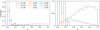 |
Fig. 9. Eccentricity distributions of the identified OB+BH systems for different BH-formation mechanisms. Right panel: zoomed-in view of the y axis of the left panel. |
Different kick mechanisms also result in different observed period distributions. Period distributions for the different BH-formation scenarios are shown in Fig. 10. In case of no kick, we expect to observe more long-period systems, whereas for the NS kick scenario more short-period systems and almost no very long-period systems are expected. This is because long-period systems are more easily disrupted by a kick as they are less gravitationally bound than short period systems. The hatched regions in Fig. 10 indicate the orbital period range (P ≤ 10 days) for which wind-fed or Roche-lobe filling X-ray binaries (e.g., Cyg X1) may occur. However, Sen et al. (2021) predict that even in this region, not many OB+BH binaries will be X-ray bright.
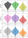 |
Fig. 10. Violin plots for the periods of different BH-formation scenarios, indicated on the x axis. The filled regions are (vertical) probability density plots, which are mirrored over the vertical solid black line. The mean of the periods is indicated with a black horizontal bar. Hatched regions correspond to possible wind-fed or Roche-lobe overfilling X-ray binaries. |
Different explosion mechanisms lead to distinct distributions of the BH masses of the identified OB+BH systems, shown in Fig. 11. Here, the distributions are smoothed with a Gaussian bandwidth of 0.3 to focus on their overall shape, instead of their discreteness (originating from the discrete distribution of the main-sequence primary star masses in the simulations). We can see that in the rapid (delayed) explosion scenarios, we do not see a continuous distribution as in the case of full collapse, but rather a bimodal (trimodal) one, with a dearth of BHs around 10 (10 and 13) M⊙ (the dashed lines in Fig. 11) due to the mass lost in the SN. Moreover, for the delayed explosion scenario, we expect BH masses in the mass gap below 5 M⊙, which is not expected for the other two scenarios. Finally, in the case of a NS kick, all scenarios tend towards larger BH masses.
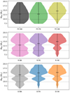 |
Fig. 11. Same as Fig. 10 but for the masses of the BHs. The distributions shown here are smoothed. The dashed lines correspond to masses around 10 and 13 M⊙. |
Furthermore, the correlation between the period and the mass ratio can also provide information on the kick scenario, as Fig. 12 shows. The lines in the figure show the modes of the columns in the two-dimensional distributions in the bottom panels of Fig. F.1 and the shaded regions represent the period boundaries in which 68% of the systems fall. The difference between the NK and FK scenarios is subtle. For the NK scenario, we expect for the low-mass-ratio systems more detections with longer periods (P > 100 days) than shorter periods, gradually lowering the most expected periods as the mass ratio increases. The FK scenario seems to favour a slightly flatter distribution. In the HK scenario, longer periods appear to be less common, as expected and already seen from Fig. 10. This is because longer period systems are more easily disrupted by kicks as they are less gravitationally bound. A similar reasoning can be made for the correlation between the mass of the LC and the period. Here, the relative amount of long-period systems amongst the lower-mass LCs rapidly decreases between the NK, FK, and HK scenarios (see Fig. F.2).
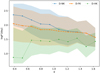 |
Fig. 12. Correlation between the mass ratio, q, and period, P, of the identified OB+BH systems for the three different kick scenarios combined with the delayed SN mechanism. Lines represent the modes of the two-dimensional distributions in Fig. F.1, and the shaded regions account for 68% of the systems. |
This experiment shows that we should be able to distinguish between different BH-formation scenarios from the distributions of the eccentricity, period, and BH mass. However, there are certain uncertainties embedded in these distributions. Therefore, if the distributions of the observed parameters follow the predicted distributions of one of the BH-formation scenarios mentioned here, we need to carefully take into consideration any uncertainties possibly affecting the predicted distributions. For example, it is sometimes argued that stars more massive than 30 M⊙ do not expand much during their evolution, such that mass transfer will never be initiated before the BH formation of the primary (Gilkis et al. 2021). Hence, the system will not be circularised by mass transfer. For wider systems in which tides do not play a significant role, we, for example, will observe the initial eccentricity in the direct-collapse scenario. If this is indeed the case, we might observe large eccentricities that are not related to the BH-formation scenario and originate in the natal eccentricity distribution.
6.3. Uncertainties on the results
The analysis performed in this paper has not taken into account uncertainties on the observed parameters. However, observational uncertainties on α, ϖ, M1, P, and the apparent G-band magnitude result in uncertainties on the binary detection fraction from Gaia and the identification fraction in the AMRF diagram. There are two types of contributions to the uncertainties: true-negatives and false-positives. The first are OB+BH systems that are not detected by our methods, and the latter are OB+MS systems that are falsely classified as OB+BH systems in the AMRF diagram. Although, theoretically OB+MS systems all lie below the maximum of the main-sequence-AMRF curve, observational uncertainties could cause some OB+MS systems to falsely pop up above the triple-AMRF. Below, we investigate the effect of both contributions through a Monte Carlo simulation and show that the results presented in Sect. 5 are robust.
6.3.1. True negatives
The estimated number of OB+BH systems in the ALS II is around 300. Hence, we drew a sample of 300 OB+BH systems from the simulations and obtained parameters according to the methods explained in Sect. 3.
For the Monte Carlo simulation, 1000 samples were simulated with new observed parameters, drawn from a normal distribution around the true value with a sigma corresponding to the uncertainty on the parameter. The parameter with the largest uncertainty will most likely be the mass of the primary, since there is no visible binary companion to accurately determine the primary mass from. Therefore, a conservative uncertainty of 50% was assumed for the mass of the LC, with a lower limit of 7 M⊙. The uncertainties on α and ϖ were both determined by the Gaia precision at the true magnitude, where we assumed Gaia will always return α > 0 but also that ϖ > 0 since the ALS II systems have high-quality data. A standard deviation of 10% was used for the period, with a lower limit of 0 days. The uncertainty on G was taken to be 0.01mag (Kourniotis et al. 2014).
The detection and identification of the new systems as binaries followed the same observational constraints as explained in Sect. 3 and Sect. 4, respectively. Using again the conservative criterion, the average fraction of OB+BH systems detected by Gaia is 77.4 %, where the errors represent a 99.7% (3-σ) confidence interval. The average AMRF completeness is 82.9
 % within a 99.7% confidence interval. Ultimately, we find that we could identify 64.2
 % of the OB+BH systems that are observed by Gaia, again within a 99.7% confidence interval. Although the AMRF completeness is smaller than the one obtained in Sect. 5, the total fraction of identified systems is still compatible with the one obtained in Sect. 5. Repeating this experiment multiple times with a different sample of 300 OB+BH systems results in similar conclusions. While the detection fraction and AMRF completeness may vary, the overall identification fraction amongst the observed sources are compatible with one another.
6.3.2. False positives
Similarly, we investigated how many OB+MS systems would have an observational 𝒜 larger than the maximum of the triple-AMRF. Assuming continuous star formation and an initial binary fraction of 70%, approximately 50% of massive stars are currently in binaries with a main-sequence companion, while 20% are post-interaction binaries, and 30% are single (de Mink et al. 2014). This results in about 7000 OB+MS systems present in the ALS II. These 7000 OB+MS systems were drawn from the distributions determined by Sana et al. (2012) and a second set of initial systems was drawn from the distributions presented in Moe & Di Stefano (2017). In both scenarios, primary masses followed the Salpeter (1955) initial mass function, ranging from 8 to 60 M⊙.
Performing multiple monte carlo simulations using the same uncertainties as for the OB+BH systems, we find that, at most, four such OB+MS systems will have an observational 𝒜 larger than the maximum of the triple-AMRF. However, taking into account the uncertainty on 𝒜, none of these systems end up having 𝒜 − σ𝒜 > 𝒜triple, such that, in principle, they would not be classified as OB+BH systems. Hence, the contribution of OB+MS to the number of false positives to the sample should be negligible.
In principle, one would want to check the contribution of triples to the number of false positives. However, in reality, the distributions of their parameters are not well known (see e.g., Duchêne & Kraus 2013). Performing such analysis is hence beyond the scope of this research. However, it should be taken into account for further analysis.
6.4. OB+BH systems in the extended mission
We can also investigate how the detection of OB+BH systems (in the FC-NK scenario) would improve in the extended 10-year mission, which is already ongoing with a mid-term review in 20222. Assuming that the precision at the end of the extended 10-year mission will not be limited by instrumentation and that the number of observations doubles with respect to the 5-year mission, we can scale the precision with a factor  . The conservative upper limit on the period increases to 10 yr.
The fraction of systems detected by Gaia slightly increases to 88.3% of the sampled OB+BH systems. The AMRF completeness is still fairly high with a value of 80.0%, yielding a conservative identification of 70.7% of the sampled OB+BH systems), which is 1% more than at the end of the 5-year mission. In terms of true numbers, this would mean an identification of ∼200 OB+BH binaries of the sources in the ALS II, not including the bright sources. An overview of the distributions of the identified OB+BH binaries is given in Fig. G.1. As a reference, the distributions of the identified systems in DR3 and DR4 are also shown. While the contribution of the extended mission is small in absolute numbers, it will allow us to probe the longer end of the period distribution (P > 5 yr) where critical signatures of the kick scenario are expected (see Fig. 10).
The number of sources in the Gaia catalogue has increased over different data releases. On the one hand there is the better precision with which sources can be observed. On the other hand, for very faint and bright sources, more data also means a (better) detection. On top of that, the known catalogue of massive stars will increase over time (e.g., the ALS III). Therefore, the estimated number might even be much higher at the end of the extended mission, as even more sources could be observed by Gaia and uncertainties on the observed parameters could become smaller.
7. Summary
We have used the massive star evolution computations of Langer et al. (2020), which assume a direct collapse and no natal kick upon BH formation, as the fiducial case to study the expected distribution of OB+BH binaries (i.e. the BH + BH/NS progenitors) in the Milky Way. In particular, we have investigated how many OB+BH systems that have been observed by Gaia will be detected as binaries, both in DR3 and DR4. Using the distance distribution of known OB stars in the ALS II, we find that, in DR3, 76.5% of the OB+BH systems observed by Gaia will be classified as binaries in the Gaia catalogue in the conservative case. In DR4, this number increases to 85.0%. These fractions can change when using a significantly different distance distribution.
We have also adapted the method established by Shahaf et al. (2019) for massive primary components to identify the detected OB+BH binaries. We can identify 88.7% and 82.3% of the OB+BH binaries that are detected by Gaia as binaries in DR3 and DR4, respectively. This ultimately leads to the identification of 67.8% of the OB+BH binaries observed by Gaia in DR3, while 69.9% of the observed OB+BH binaries can be identified in DR4. Translating these fractions to an absolute number of OB+BH systems in the ALS II, around 190 OB+BH binaries can already be identified as such in DR3, increasing the known (quiescent) OB+BH binaries by a factor of more than 20. An additional ∼5 OB+BH systems will be identifiable in DR4, mostly with short (P ≲ 10 d) or long periods (P ≳ 1000 d).
We also found that different BH-formation mechanisms result not only in different detection fractions, but also in distinct distributions of BH masses, orbital periods, and eccentricities. However, relating the distributions of the identified OB+BH systems directly to the BH-formation mechanism should be done with caution as different scenarios may occur for different mass regimes. Nonetheless, our results predict that both the numbers and the distributions of orbital properties of the detected OB+BH systems will provide crucial observational constraints to the collapse scenario and the formation of BH+BH/NS progenitors.
We have shown that the identifiable fraction of OB+BH systems is robust. Hence, the number of OB+BH system identifications opens up the possibility of drawing profound conclusions on the physics of BH formation.
Acknowledgments
S. J. acknowledges support from the FWO PhD fellowship under project 11E1721N. This project has received funding from the European Research Council (ERC) under the European Union’s Horizon 2020 research and innovation programme (grant agreement n° 772225/MULTIPLES). This research was supported by Grant No. 2016069 of the United States-Israel Binational Science Foundation (BSF), and by Grant No. I-1498-303.7/2019 of the German-Israeli Foundation for Scientific Research and Development (GIF).
References
- Abbott, B. P., Abbott, R., Abbott, T. D., et al. 2016, ApJ, 818, L22 [Google Scholar]
- Abbott, B. P., Abbott, R., Abbott, T. D., et al. 2017, ApJ, 848, L12 [Google Scholar]
- Abdul-Masih, M., Banyard, G., Bodensteiner, J., et al. 2020, Nature, 580, E11 [Google Scholar]
- Adelman, S. J. 2004, in The A-Star Puzzle, eds. J. Zverko, J. Ziznovsky, S. J. Adelman, & W. W. Weiss, 224, 1 [NASA ADS] [Google Scholar]
- Bodensteiner, J., Shenar, T., Mahy, L., et al. 2020, A&A, 641, A43 [NASA ADS] [CrossRef] [EDP Sciences] [Google Scholar]
- Boyajian, T. S., McAlister, H. A., van Belle, G., et al. 2012a, ApJ, 746, 101 [Google Scholar]
- Boyajian, T. S., von Braun, K., van Belle, G., et al. 2012b, ApJ, 757, 112 [Google Scholar]
- Breivik, K., Chatterjee, S., & Larson, S. L. 2017, ApJ, 850, L13 [CrossRef] [Google Scholar]
- Breivik, K., Chatterjee, S., & Andrews, J. J. 2019, ApJ, 878, L4 [NASA ADS] [CrossRef] [Google Scholar]
- Bresolin, F., Crowther, P. A., & Puls, J. 2008, in Massive Stars as Cosmic Engines, IAU Symp., 250 [Google Scholar]
- Brott, I., Evans, C. J., Hunter, I., et al. 2011, A&A, 530, A116 [NASA ADS] [CrossRef] [EDP Sciences] [Google Scholar]
- Brown, G. E., & Bethe, H. A. 1994, ApJ, 423, 659 [NASA ADS] [CrossRef] [Google Scholar]
- Casares, J., Negueruela, I., Ribó, M., et al. 2014, Nature, 505, 378 [Google Scholar]
- Choi, J., Dotter, A., Conroy, C., et al. 2016, ApJ, 823, 102 [Google Scholar]
- Corral-Santana, J. M., Casares, J., Muñoz-Darias, T., et al. 2016, A&A, 587, A61 [NASA ADS] [CrossRef] [EDP Sciences] [Google Scholar]
- Crowther, P. A., & Hadfield, L. J. 2006, A&A, 449, 711 [NASA ADS] [CrossRef] [EDP Sciences] [Google Scholar]
- de Mink, S. E., Sana, H., Langer, N., Izzard, R. G., & Schneider, F. R. N. 2014, ApJ, 782, 7 [Google Scholar]
- Dotter, A. 2016, ApJS, 222, 8 [Google Scholar]
- Duchêne, G., & Kraus, A. 2013, ARA&A, 51, 269 [Google Scholar]
- El-Badry, K., & Quataert, E. 2020, MNRAS, 493, L22 [NASA ADS] [CrossRef] [Google Scholar]
- Ertl, T., Woosley, S. E., Sukhbold, T., & Janka, H. T. 2020, ApJ, 890, 51 [CrossRef] [Google Scholar]
- Everall, A., Boubert, D., Koposov, S. E., Smith, L., & Holl, B. 2021, MNRAS, 502, 1908 [CrossRef] [Google Scholar]
- Fryer, C. L., Belczynski, K., Wiktorowicz, G., et al. 2012, ApJ, 749, 91 [Google Scholar]
- Gaia Collaboration (Prusti, T., et al.) 2016, A&A, 595, A1 [NASA ADS] [CrossRef] [EDP Sciences] [Google Scholar]
- Gaia Collaboration (Brown, A. G. A., et al.) 2021, A&A, 649, A1 [NASA ADS] [CrossRef] [EDP Sciences] [Google Scholar]
- Giesers, B., Dreizler, S., Husser, T.-O., et al. 2018, MNRAS, 475, L15 [NASA ADS] [CrossRef] [Google Scholar]
- Gilkis, A., Shenar, T., Ramachandran, V., et al. 2021, MNRAS, 503, 1884 [NASA ADS] [CrossRef] [Google Scholar]
- Gillon, M., Demory, B.-O., Van Grootel, V., et al. 2017, Nat. Astron., 1, 0056 [Google Scholar]
- Gould, A., & Salim, S. 2002, ApJ, 572, 944 [NASA ADS] [CrossRef] [Google Scholar]
- Hainich, R., Pasemann, D., Todt, H., et al. 2015, A&A, 581, A21 [NASA ADS] [CrossRef] [EDP Sciences] [Google Scholar]
- Heckman, T. M., Armus, L., & Miley, G. K. 1990, ApJS, 74, 33 [Google Scholar]
- Hobbs, G., Lorimer, D. R., Lyne, A. G., & Kramer, M. 2005, MNRAS, 360, 974 [Google Scholar]
- Holgado, G., Simón-Díaz, S., Haemmerlé, L., et al. 2020, A&A, 638, A157 [NASA ADS] [CrossRef] [EDP Sciences] [Google Scholar]
- Hopkins, P. F. 2014, Am. Astron. Soc. Meeting Abstr., 224, 215.06 [NASA ADS] [Google Scholar]
- Irrgang, A., Geier, S., Kreuzer, S., Pelisoli, I., & Heber, U. 2020, A&A, 633, L5 [NASA ADS] [CrossRef] [EDP Sciences] [Google Scholar]
- Jayasinghe, T., Stanek, K. Z., Thompson, T. A., et al. 2021, MNRAS, 504, 2577 [NASA ADS] [CrossRef] [Google Scholar]
- Kaltenegger, L., & Traub, W. A. 2009, ApJ, 698, 519 [Google Scholar]
- Kervella, P., Mérand, A., Pichon, B., et al. 2008, A&A, 488, 667 [NASA ADS] [CrossRef] [EDP Sciences] [Google Scholar]
- Klencki, J., Nelemans, G., Istrate, A. G., & Chruslinska, M. 2021, A&A, 645, A54 [EDP Sciences] [Google Scholar]
- Kourniotis, M., Bonanos, A. Z., Soszyński, I., et al. 2014, A&A, 562, A125 [NASA ADS] [CrossRef] [EDP Sciences] [Google Scholar]
- Kruckow, M. U., Tauris, T. M., Langer, N., et al. 2016, A&A, 596, A58 [NASA ADS] [CrossRef] [EDP Sciences] [Google Scholar]
- Langer, N., Schürmann, C., Stoll, K., et al. 2020, A&A, 638, A39 [NASA ADS] [CrossRef] [EDP Sciences] [Google Scholar]
- Laplace, E., Justham, S., Renzo, M., et al. 2021, A&A, 656, A58 [NASA ADS] [CrossRef] [EDP Sciences] [Google Scholar]
- Lennon, D. J., Maíz Apellániz, J., Irrgang, A., et al. 2021, A&A, 649, A167 [NASA ADS] [CrossRef] [EDP Sciences] [Google Scholar]
- LIGO Scientific Collaboration & Virgo Collaboration (Abbott, P., et al.) 2016, Phys. Rev. Lett., 116, 241103 [NASA ADS] [CrossRef] [Google Scholar]
- Lindegren, L., Klioner, S. A., Hernández, J., et al. 2021, A&A, 649, A2 [EDP Sciences] [Google Scholar]
- Liu, J., Zhang, H., Howard, A. W., et al. 2019, Nature, 575, 618 [Google Scholar]
- Liu, J., Zheng, Z., Soria, R., et al. 2020, ApJ, 900, 42 [Google Scholar]
- Marchant, P., Pappas, K. M. W., Gallegos-Garcia, M., et al. 2021, A&A, 650, A107 [NASA ADS] [CrossRef] [EDP Sciences] [Google Scholar]
- Martins, F., Schaerer, D., & Hillier, D. J. 2005, A&A, 436, 1049 [NASA ADS] [CrossRef] [EDP Sciences] [Google Scholar]
- Mashian, N., & Loeb, A. 2017, MNRAS, 470, 2611 [NASA ADS] [CrossRef] [Google Scholar]
- Mazeh, T., & Faigler, S. 2020, MNRAS, 498, L58 [NASA ADS] [CrossRef] [Google Scholar]
- Moe, M., & Di Stefano, R. 2017, ApJS, 230, 15 [Google Scholar]
- Mokiem, M. R., de Koter, A., Vink, J. S., et al. 2007, A&A, 473, 603 [NASA ADS] [CrossRef] [EDP Sciences] [Google Scholar]
- Pantaleoni González, M., Maíz Apellániz, J., Barbá, R. H., & Reed, B. C. 2021, MNRAS, 504, 2968 [CrossRef] [Google Scholar]
- Paxton, B., Bildsten, L., Dotter, A., et al. 2011, ApJS, 192, 3 [Google Scholar]
- Pols, O. 2011, Binary Stars, Astronomical Institute Utrecht, online access: https://www.astro.ru.nl/~onnop/education/binaries_utrecht_notes/ [Google Scholar]
- Reed, C. 2005, VizieR Online Data Catalog, V/125 [Google Scholar]
- Rivinius, T., Baade, D., Hadrava, P., Heida, M., & Klement, R. 2020, A&A, 637, L3 [NASA ADS] [CrossRef] [EDP Sciences] [Google Scholar]
- Sabín-Sanjulián, C., Simón-Díaz, S., Herrero, A., et al. 2017, A&A, 601, A79 [NASA ADS] [CrossRef] [EDP Sciences] [Google Scholar]
- Salpeter, E. E. 1955, ApJ, 121, 161 [Google Scholar]
- Samland, M. 1998, ApJ, 496, 155 [NASA ADS] [CrossRef] [Google Scholar]
- Sana, H., de Mink, S. E., de Koter, A., et al. 2012, Science, 337, 444 [Google Scholar]
- Sana, H., Le Bouquin, J. B., Lacour, S., et al. 2014, ApJS, 215, 15 [Google Scholar]
- Schneider, F. R. N., Podsiadlowski, P., & Müller, B. 2021, A&A, 645, A5 [NASA ADS] [CrossRef] [EDP Sciences] [Google Scholar]
- Sen, K., Xu, X. T., Langer, N., et al. 2021, A&A, 652, A138 [NASA ADS] [CrossRef] [EDP Sciences] [Google Scholar]
- Shahaf, S., Mazeh, T., Faigler, S., & Holl, B. 2019, MNRAS, 487, 5610 [NASA ADS] [CrossRef] [Google Scholar]
- Shapiro, S. L., & Teukolsky, S. A. 1983, Black holes, white dwarfs, and neutron stars: the physics of compact objects [Google Scholar]
- Shenar, T., Bodensteiner, J., Abdul-Masih, M., et al. 2020a, A&A, 639, L6 [EDP Sciences] [Google Scholar]
- Shenar, T., Gilkis, A., Vink, J. S., Sana, H., & Sander, A. A. C. 2020b, A&A, 634, A79 [NASA ADS] [CrossRef] [EDP Sciences] [Google Scholar]
- Silaj, J., Jones, C. E., Sigut, T. A. A., & Tycner, C. 2014, ApJ, 795, 82 [Google Scholar]
- Spitzer, L. 1978, Physical processes in the interstellar medium [Google Scholar]
- Straizys, V., & Kuriliene, G. 1981, Ap&SS, 80, 353 [CrossRef] [Google Scholar]
- Thompson, T. A., Kochanek, C. S., Stanek, K. Z., et al. 2019, Science, 366, 637 [NASA ADS] [CrossRef] [Google Scholar]
- Timmes, F. X., Woosley, S. E., & Weaver, T. A. 1996, ApJ, 457, 834 [NASA ADS] [CrossRef] [Google Scholar]
- Trimble, V. L., & Thorne, K. S. 1969, ApJ, 156, 1013 [Google Scholar]
- van den Heuvel, E. P. J. 1992, Endpoints of stellar evolution: the incidence of stellar mass black holes in the Galaxy., Environment Observation and Climate Modelling Through International Space Projects [Google Scholar]
- Vardavas, I. M., & Taylor, F. W. 2011, Radiation and Climate: Atmospheric Energy Budget from Satellite Remote Sensing (Oxford: Oxford Science Publications) [Google Scholar]
- Vink, J. S., de Koter, A., & Lamers, H. J. G. L. M. 2001, A&A, 369, 574 [NASA ADS] [CrossRef] [EDP Sciences] [Google Scholar]
- Wang, S., & Chen, X. 2019, ApJ, 877, 116 [Google Scholar]
- Wiktorowicz, G., Wyrzykowski, Ł., Chruslinska, M., et al. 2019, ApJ, 885, 1 [NASA ADS] [CrossRef] [Google Scholar]
- Woosley, S. E. 2019, ApJ, 878, 49 [Google Scholar]
- Yalinewich, A., Beniamini, P., Hotokezaka, K., & Zhu, W. 2018, MNRAS, 481, 930 [NASA ADS] [CrossRef] [Google Scholar]
- Yamaguchi, M. S., Kawanaka, N., Bulik, T., & Piran, T. 2018, ApJ, 861, 21 [NASA ADS] [CrossRef] [Google Scholar]
Appendix A: The period change due to mass loss
We derive here an expression for the final period of a binary system, where the change in period is only caused by mass-loss through winds of the components. The angular momentum loss of a non-eccentric system (e = 0, ė = 0) is given by
where for notation simplicity we have used Mtot = M1 + M2 and Ṁtot = Ṁ1 + Ṁ2. The specific orbital angular momentum is given by
where i and j are the components of the binary system. This expression assumes that the radius of component i is much smaller than its Roche-lobe radius, such that spin-angular momentum can be neglected.
The angular momentum loss can hence be written as  . Using this expression in Eq. (A.1) gives
After some simplification, this becomes
Solving this expression gives us Eq. (4).
Appendix B: Mass and period differences between the LMC and the Milky Way
Figure B.1 presents the distributions of the masses of the LCs and BHs, the mass ratios, and periods of the OB+BH systems in the LMC compared to those in the Milky Way.
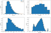 |
Fig. B.1. Difference in distributions of the LC (top-left) and BH (top-right) mass, the mass-ratio (MBH/MOB, bottom-left), and the period (bottom-right) of the OB+BH systems in the LMC (filled) and Milky Way (open) after applying the corrections mentioned in Sect. 2.2. The mass distributions of the LC are almost identical and minor changes occur due to the relatively weak winds of the main-sequence LC, whereas the masses of the BHs are shifted towards lower values due to the powerful stellar winds experienced by the post-mass-transfer components. Hence, the mass ratios have shifted towards lower values as well. The orbits have slightly widened. |
Appendix C: The semi-major axis of the projected orbit
We derive an expression for the semi-major axis of the projected orbit, starting from the general equation of an ellipse. The general form of an ellipse whose semi-major (a) and semi-minor (b) axis are not aligned with the axes of the reference frame is given by

with
where xc and yc are the coordinates of the centre and θ is the angle between a and the horizontal axis of the reference frame. For an ellipse centred at the origin, 𝒟, ℰ = 0 and ℱ = −a2b2 = ℬ2/4 − 𝒜𝒞. The semi-major axis of the ellipse is given by
We can take three points on an ellipse centred at the origin with coordinates (x1, y1), (x2, y2), and (x3, y3). By using Eq. (C.1) for each of the three points and solving the three equations, the constants 𝒜, ℬ, and 𝒞 can be written as
with
We want to obtain an expression for the semi-major axis of the projected ellipse as a function of the orbital parameters i, Ω, and ω, independent of the three points chosen. The central coordinates of the projected ellipse, using Eq. (7), are xc = −Ae and yc = −Be. We can transform the coordinates of the projected ellipse to x − xc and y − yc, such that we implicitly have an ellipse centred at the origin. By doing this, we can use Eq. (C.1) for a general ellipse centred at the origin. Moreover, the projected coordinates simplify to
Let us start by investigating the variable v in Eq. (C.5). The Thiele-Innes constants A, B, F, and G (Eq. (6)) of any coordinate on the ellipse are equal to each other. Hence, we want to show that v is independent of the eccentric anomaly E, as this is the only parameter that changes between different points on the ellipse. One way of verifying this, is by showing that the partial derivative of v with respect to all E’s is equals to zero such that for each point i we have ∂Ei(v) = 0. If we call n the numerator and d the denominator, this is equivalent to ∂Ei(n)/∂Ei(d) = n/d. By calculating both d∂Ei(n) and n∂Ei(d) of v, it can be shown that v is independent of E1, E2, and E3. We can hence take E1 = 0, E2 = π/3, and E3 = 2π/3 to find a simple expression for v as a function of A, B, F, and G,
where for simplicity of notation we have  and
and  .
.
By following the same method and using the simplified version of v, it can be shown that w is also independent of the choice of E1 and E2. We take E1 = 0 and E2 = π/2 and simplify w to
We now only need to show that ℬ is also constant. The same method can again be used. We use Eqs. (C.7,C.8) and take E1 = 0, such that
The equation for the semi-major axis of the projected ellipse ‘centred’ at the origin is obtained by using the above three expressions in Eq. (C.4) and Eq. (C.3),
where w and v are now constants only dependent on the orbital parameters through the Thiele-Innes constants. For circular orbits, e = 0 and we have F′=F and G′=G. By working out each of the terms in Eq. (C.10), it can be shown that the semi-major axis of the projected ellipse is equal to the true semi-major axis of the circular orbit.
Appendix D: Masses, effective temperatures, and radii
Table D.1 shows the literature data obtained for main-sequence dwarf stars.
Masses, effective temperatures and radii of dwarf stars used for the fitting of the mass-magnitude relation in Sect. 4.1.
Appendix E: Corner plots for the detected systems in Gaia
Figures E.1 and E.2 show corner plots for the parameters of OB+BH systems in DR3 and DR4, respectively, after applying several observational constraints.
 |
Fig. E.1. Corner plot for the OB+BH systems in Gaia in DR3. Black represents the underlying distribution of the simulated systems, orange are the systems which are detected by Gaia (i.e. have a magnitude 6 < G < 20), and cyan are the detected systems in the conservative case. The under-diagonal plots are 2D histograms showing the underlying distribution. |
Appendix F: Mass and period distribution for different BH formation mechanisms
Figures F.1 and F.2 show the correlation distributions between the period and the mass ratio, and, the period and mass of the LC, respectively, for the different BH-formation scenarios.
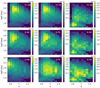 |
Fig. F.1. Two-dimensional histograms of the mass ratio q and the period P. The histograms look similar for different collapse scenarios, but not for different kick scenarios. |
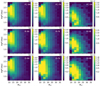 |
Fig. F.2. Two-dimensional histograms of the mass of the LC MLC and the period P. The histograms look similar for different collapse scenarios, but not for different kick scenarios. |
Appendix G: Mass and period distribution in the 10-yr mission
Figure G.1 shows the distributions in masses and periods expected for the identifiable OB+BH systems at the end of the extended 10-yr mission.
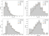 |
Fig. G.1. Same as Fig. 8, but only for the identified OB+BH binaries at the end of the extended 10-yr mission. The distributions of identified systems in the other two data releases are also shown as a reference. |
All Tables
Fit parameters for the mass-magnitude relation of dwarfs in different mass regimes.
Fraction of surviving and identified systems for different BH-formation scenarios.
Masses, effective temperatures and radii of dwarf stars used for the fitting of the mass-magnitude relation in Sect. 4.1.
All Figures
|
Fig. 1. Distances of the massive OB stars in the ALS II (left), and absolute (open blue) and apparent (open orange) magnitudes of the full sample of simulated OB+BH systems (right). The right panel also shows the absolute and apparent magnitudes of the massive stars in the ALS II (dashed black and grey, respectively). |
| In the text | |
|
Fig. 2. Orbital projection for an example of a MS+BH system with MBH = 10 M⊙, MLC = 15 M⊙, aLC = 1.17 au, and e = 0.6. The solid ellipse represents the true orbit, with the semi-major axis shown as the two stars connected by a red line. The dashed ellipse shows the orbit projected with i = 60°, Ω = 52.9°, and ω = 242.4°. The projected semi-major axis is shown as a dashed red line. The blue triangles connected with a dashed line show the semi-major axis of the projected orbit, α. |
| In the text | |
|
Fig. 3. G-band magnitudes for dwarfs in the mass range 0.2–55.67 M⊙ obtained from the literature (see Table D.1). The masses are shown on a logarithmic scale. The fit is shown with a solid red line. Grey vertical lines indicate the fitted regions. |
| In the text | |
|
Fig. 4. Different theoretical AMRFs for three different primary masses: 9 M⊙ (blue), 20 M⊙ (orange), and 30 M⊙ (grey). The solid black line shows the theoretical AMRF for MS+BH systems, the dotted curves are for main-sequence binaries, and dashed curves are for triple main-sequence systems. Different classes are also indicated for the 30 M⊙ primary by the horizontal dotted lines at the maxima of the triple-AMRF and the main-sequence AMRF (Class III: identifiable OB+BH systems, Class II: triple main-sequence or OB+BH systems, Class I: OB+OB binaries, triple main-sequence systems, or OB+BH binaries). |
| In the text | |
|
Fig. 5. Astrometric signal and magnitudes of the simulated OB+BH systems for DR3 (left) and for DR4 (right). The top panels are with a colour-coded period, and the bottom panels are density plots. Systems with periods longer than the upper limit of the respective data release are not shown. The vertical dotted lines in the panels show the limiting Gaia magnitude. From top to bottom, the meaning of the different entries in the legend is the fraction of OB+BH systems in total (by definition 100%), those with a G-band magnitude between 6 and 20 mag, those with a period below the upper limit, and those that have an astrometric signal larger than 1σ or 3σ, respectively. Systems that pass a certain criterion also need to have passed the criteria mentioned above it. The two higher-density regions in the bottom plot originate in the underlying period distribution related to the mass transfer event (see also the upper panel of Fig. 6 in Langer et al. 2020). Systems undergoing Case A mass transfer are found at shorter periods (the bottom region), and systems going through Case B mass transfer end up with higher periods (upper region). |
| In the text | |
|
Fig. 6. Masses of the components and the periods as a function of the astrometric signal. The underlying distributions (those of Langer et al. 2020) are shown with black dots and overplotted with those systems having 6 < G < 20 (orange stars). On top is the subset of systems that are detected in the conservative case (i.e. α > 3σ and a period lower than the imposed upper limit; cyan triangles). The left panels are for DR3 and the right panels for DR4. The discrete BH masses come from the discrete main-sequence primary masses in the simulations of Langer et al. (2020). |
| In the text | |
|
Fig. 7. Distribution of 𝒜 for the systems classified as a binary by Gaia. The left panel is for DR3 and the right panel for DR4. The curves are the same as in Fig. 4 (legend on top). Systems with 𝒜 − σ𝒜 > 𝒜triple (Class III) are represented by the purple open histogram, and systems with 𝒜 − σ𝒜 ≤ 𝒜triple (non-Class III) are shown with an orange filled histogram. Bins are 0.025 in width. The open histograms account for 88.7% and 82.3% of the total number of detected systems in the left and right panel, respectively. |
| In the text | |
|
Fig. 8. Distribution of MLC (top left), MBH (top right), q (bottom left), and P (bottom right) in DR3 and DR4. In the legend, ‘Underlying’ is the distribution of all simulated OB+BH systems, ‘Detected’ are those systems detected as binaries by Gaia, and ‘Identified’ are Class III systems (i.e. confirmed OB+BH systems). The last systems are the observational distributions that can be expected to be constructed using the OB+BH systems identified in the respective data release. |
| In the text | |
|
Fig. 9. Eccentricity distributions of the identified OB+BH systems for different BH-formation mechanisms. Right panel: zoomed-in view of the y axis of the left panel. |
| In the text | |
|
Fig. 10. Violin plots for the periods of different BH-formation scenarios, indicated on the x axis. The filled regions are (vertical) probability density plots, which are mirrored over the vertical solid black line. The mean of the periods is indicated with a black horizontal bar. Hatched regions correspond to possible wind-fed or Roche-lobe overfilling X-ray binaries. |
| In the text | |
|
Fig. 11. Same as Fig. 10 but for the masses of the BHs. The distributions shown here are smoothed. The dashed lines correspond to masses around 10 and 13 M⊙. |
| In the text | |
|
Fig. 12. Correlation between the mass ratio, q, and period, P, of the identified OB+BH systems for the three different kick scenarios combined with the delayed SN mechanism. Lines represent the modes of the two-dimensional distributions in Fig. F.1, and the shaded regions account for 68% of the systems. |
| In the text | |
|
Fig. B.1. Difference in distributions of the LC (top-left) and BH (top-right) mass, the mass-ratio (MBH/MOB, bottom-left), and the period (bottom-right) of the OB+BH systems in the LMC (filled) and Milky Way (open) after applying the corrections mentioned in Sect. 2.2. The mass distributions of the LC are almost identical and minor changes occur due to the relatively weak winds of the main-sequence LC, whereas the masses of the BHs are shifted towards lower values due to the powerful stellar winds experienced by the post-mass-transfer components. Hence, the mass ratios have shifted towards lower values as well. The orbits have slightly widened. |
| In the text | |
|
Fig. E.1. Corner plot for the OB+BH systems in Gaia in DR3. Black represents the underlying distribution of the simulated systems, orange are the systems which are detected by Gaia (i.e. have a magnitude 6 < G < 20), and cyan are the detected systems in the conservative case. The under-diagonal plots are 2D histograms showing the underlying distribution. |
| In the text | |
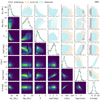 |
Fig. E.2. Same as Fig. E.1 but for DR4. |
| In the text | |
|
Fig. F.1. Two-dimensional histograms of the mass ratio q and the period P. The histograms look similar for different collapse scenarios, but not for different kick scenarios. |
| In the text | |
|
Fig. F.2. Two-dimensional histograms of the mass of the LC MLC and the period P. The histograms look similar for different collapse scenarios, but not for different kick scenarios. |
| In the text | |
|
Fig. G.1. Same as Fig. 8, but only for the identified OB+BH binaries at the end of the extended 10-yr mission. The distributions of identified systems in the other two data releases are also shown as a reference. |
| In the text | |
Current usage metrics show cumulative count of Article Views (full-text article views including HTML views, PDF and ePub downloads, according to the available data) and Abstracts Views on Vision4Press platform.
Data correspond to usage on the plateform after 2015. The current usage metrics is available 48-96 hours after online publication and is updated daily on week days.
Initial download of the metrics may take a while.