| Issue |
A&A
Volume 690, October 2024
|
|
|---|---|---|
| Article Number | A48 | |
| Number of page(s) | 20 | |
| Section | Galactic structure, stellar clusters and populations | |
| DOI | https://doi.org/10.1051/0004-6361/202450448 | |
| Published online | 27 September 2024 | |
An in-depth analysis of the differentially expanding star cluster Stock 18 (Villafranca O-036) using Gaia DR3 and ground-based data
1
Centro de Astrobiología, CSIC-INTA. Campus ESAC. C, bajo del castillo s/n., 28 692 Villanueva de la Cañada, Madrid, Spain
2
Astronomy, Space Science, and Meteorology Department, Faculty of Science, Cairo University, 12613 Giza, Egypt
3
Department of Physics, College of Science, Northern Border University, Arar, Saudi Arabia
4
Department of Astronomy, National Research Institute of Astronomy and Geophysics (NRIAG), 11421 Helwan, Cairo, Egypt
5
Instituto de Astrofísica de Andalucía (IAA), CSIC, Glorieta de la Astronomía s/n., 18 008 Granada, Spain
6
Departamento de Astrofísica y Física de la Atmósfera, Universidad Complutense de Madrid, 28 040 Madrid, Spain
Received:
19
April
2024
Accepted:
22
May
2024
Abstract
Context. The Villafranca project is combining Gaia data with ground-based surveys to analyze Galactic stellar groups (clusters, associations, or parts thereof) with OB stars.
Aims. We want to analyze the poorly studied cluster Stock 18 within the Villafranca project, as it is a very young stellar cluster with a symmetrical and compact H II region around it, Sh 2-170, so it is likely to provide insights into the structure and dynamics of such objects at an early stage of their evolution.
Methods. We used Gaia astrometry, photometry, spectrophotometry, and variability data as well as ground-based spectroscopy and imaging to determine the characteristics of Stock 18. We used these data to analyze its core, massive star population, extinction, distance, membership, internal dynamics, density profile, IMF, stellar variability, and Galactic location.
Results. Stock 18 is a very young (∼1.0 Ma) cluster located at a distance of 2.91 ± 0.10 kpc and is dominated by the GLS 13 370 system, whose primary (Aa) is an O9 V star. We propose that Stock 18 was in a very compact state (∼0.1 pc) about 1.0 Ma ago and that most massive stars were ejected at that time without significantly affecting the less massive stars as a result of multi-body dynamical interactions. Different age estimates also point toward an age close to 1.0 Ma, indicating that the dynamical interactions took place very shortly after massive star formation. Well-defined expanding stellar clusters have been observed before, but none are as young as this one. If we include all of the stars, the initial mass function is top heavy, but if we discard the ejected ones, it becomes nearly canonical. Therefore, this is another example (in addition to the previous one we found – the Bermuda cluster) of (a) a very young cluster with an already evolved present day mass function (b) that has significantly contributed to the future population of free-floating compact objects. If confirmed in more clusters, the number of such compact objects may be higher in the Milky Way than previously thought. Stock 18 has a variable extinction with an average value of R5495 higher than the canonical one of 3.1. We have discovered a new visual component (Ab) in the GLS 13 370 system. The cluster is above our Galactic mid-plane, likely as a result of the Galactic warp, and it has a distinct motion with respect to its surrounding old population, which is possibly an influence of the Perseus spiral arm.
Key words: techniques: photometric / catalogs / parallaxes / proper motions / stars: luminosity function / mass function / open clusters and associations: individual: Stock 18
Corresponding author; This email address is being protected from spambots. You need JavaScript enabled to view it. .
Deceased.
© The Authors 2024
 Open Access article, published by EDP Sciences, under the terms of the Creative Commons Attribution License (https://creativecommons.org/licenses/by/4.0), which permits unrestricted use, distribution, and reproduction in any medium, provided the original work is properly cited.
This article is published in open access under the Subscribe to Open model. This email address is being protected from spambots. You need JavaScript enabled to view it. to support open access publication.
1. Introduction
The analysis of open star clusters provides a window into our comprehension of stellar evolution and the structure and evolution of the Milky Way (MW) thin disc, as they are foundational units of galaxies (Gilmore et al. 2012). The youngest open clusters, those with ages of only several Ma, are particularly interesting as their conditions are still similar to the initial ones, shedding light onto the process of star formation, and as they possess present day mass functions (PDMFs) only slightly altered from the initial one (or IMF).
The European Space Agency mission Gaia has revolutionized the study of open star clusters by providing astrometric, photometric, and spectroscopic information for almost 2 × 10⁹ sources. We are combining Gaia information with ground-based data to conduct the Villafranca project, a study of Galactic OB groups in the solar neighborhood. An OB group is a stellar ensemble born from a single cloud that may be bound (a cluster) or unbound (an association or part thereof) and that is massive and young enough to still contain one or (more typically) several OB stars. For the latter, we use the classical definition of a star with a spectral type earlier than B2 for dwarfs (luminosity class V), B5 for giants (luminosity class III), and B9 for supergiants (luminosity class I). The Villafranca project uses Gaia astrometry, photometry, and spectroscopy to derive the properties of stellar OB groups with the help of ground-based spectroscopic and photometric surveys. The first type of survey, such as the Galactic O-Star Spectroscopic Survey (GOSSS, Maíz Apellániz et al. 2011) and LiLiMaRlin (Maíz Apellániz et al. 2019a) are used to characterize the OB stars in the groups and are being combined into an umbrella project called the Alma Luminous Star (ALS) survey (Reed 2003; Pantaleoni González et al. 2021) that is analyzing tens of thousands of Local Group massive stars. The second type of survey, such as 2MASS (Skrutskie et al. 2006) and GALANTE (Maíz Apellániz et al. 2021a), are used to determine properties such as extinction for the stars in the cluster or association. In the prototype Villafranca paper (Maíz Apellániz 2019) we presented the method used to determine the group characteristics and analyzed the first two groups with O stars. In the two major Villafranca papers published so far (Maíz Apellániz et al. 2020 or Paper I and Maíz Apellániz et al. 2022a or Paper II) we analyzed a total of 26 stellar groups with O stars (Villafranca O-001 to Villafranca O-026) and their results have been used in subsequent papers to propose the phenomenon of orphan clusters (Maíz Apellániz et al. 2022b) and to recalibrate Gaia EDR3 (early third data release) astrometry (Maíz Apellániz et al. 2021d; Maíz Apellániz 2022). Since then, we have analyzed three additional Villafranca groups with O stars in Negueruela et al. (2022), Putkuri et al. (2023), Ansín et al. (2023) and we are currently writing the next major paper of the series (Molina-Lera et al. in prep. or Paper III), centered on the groups in Carina OB1. Counting all, we have studied 35 Galactic groups with O stars and another 5 with massive B stars.
Stock 18 is one of the 21 open clusters observed by Jürgen Stock (MacConnell 2006) in the early 1950s. It is included in a number of large catalogs that have derived information about open clusters (Russeil et al. 2007; Bukowiecki et al. 2011; Buckner & Froebrich 2013; Kharchenko et al. 2013; Dias et al. 2014; Joshi et al. 2016; Sampedro et al. 2017; Cantat-Gaudin & Anders 2020; Cantat-Gaudin et al. 2020) but has only been studied in depth by Roger et al. (2004), Bhatt et al. (2012) and Sinha et al. (2020). A summary of the results from those papers is given in Table 1.
Results from previous studies of Stock 18.
A look at Table 1 reveals a strong disparity in ages and distances in the first group (large catalogs) and a much better agreement in the second (dedicated studies). The disparity has been addressed in previous studies (Netopil et al. 2015 and Paper I) and is the result of several factors. The most important one is that large surveys have to make simplifying assumptions, many times ignoring significant clues about age and other parameters. Paper I also argued in favor of the positive role of Gaia but we note here that two of the dedicated papers were published before Gaia data became available and were still able to provide a good distance (within 2 sigmas of the value we derive below). Along the same lines, Mayer & Macák (1973) determined a distance of 2.99 kpc to GLS 13 370 A (=LS I +64 11 A), the only O star in the cluster (as we will see below), which is also a good value. The real problem with the distance appears to be its relationship with the age measurement, as several of the large surveys severely overestimate the latter.
The (sometimes ignored) youth of Stock 18 is readily apparent by its association with the H II region Sh 2-170 (Sharpless 1959), see Fig. 1. Sh 2-170 is a relatively compact, symmetrical, and filled H II region with a single O star located very close to its geometrical center. The WISE image, with W4 tracing the warm dust, reveals just a small cavity around the O star, a sign of extreme youth. A detailed analysis of the H II region by Roger et al. (2004) led to an age estimate of just 0.25–0.50 Ma, counting since the activation of the O star. The analysis of the PMS (pre-main sequence) population by Sinha et al. (2020) shows a peak at an age of 1 Ma with some stars as old as 7 Ma. The results in the two papers are consistent, as PMS models cannot easily discriminate age differences smaller than 1 Ma and star-formation on scales of ∼10 pc does not occur instantaneously: it is quite typical to have a cluster surrounded by a halo (or association) with a spread of ages of several million years.
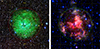 |
Fig. 1. Images of Stock 18. Left: three-channel DSS2 RGB image with the red channel corresponding to the NIR survey, the green channel to the Red survey, and the blue channel to the Blue survey. Right: WISE RGB image with the red channel corresponding to the W4 band, the green channel to a sum of the W3 and W2 bands, and the blue channel to the W1 band. In both cases, the intensity scale is logarithmic and circles with radii of 4′, 7′, and 10′ centered on the cluster are plotted |
The next section describes our data and methods, and the sections that follow those are each dedicated to a different aspect of our analysis of Stock 18: the cluster core; the massive star population, extinction, cluster membership and distance, internal cluster dynamics and structure, age and variability, IMF and cluster mass, and Galactic location. We conclude with a summary of results and an appendix with a glossary of terms.
2. Data and methods
2.1. ALS spectroscopy
Most analyses of stellar clusters with Gaia are based on data provided by the mission alone, perhaps with the additional help of other photometric surveys such as 2MASS. The problem of doing so with young groups with OB stars is that they are less “democratic” than older clusters, as the (typically few) massive stars play a disproportionately large role in the ionizing flux, stellar winds, and stellar dynamics compared to the far more numerous intermediate- and low-mass stars. In a sense, OB groups are defined by the OB stars themselves and the rest of the stars just tag along for the trip. The OB phase of a stellar group is short lived but it is the most important, as the events that take place there determine whether the rest of the stars remain bound in a cluster for the rest (or at least a significant fraction) of their lives. To study OB stars in detail, spectroscopy is needed due to the relatively poor information content of their photometry. For those reasons, in the Villafranca project we start the analysis of each group using spectroscopic information from its most outstanding denizens.
In the Villafranca project we have so far used two types of spectroscopy: Intermediate-resolution (R ∼ 2500) from GOSSS and high-resolution (R ≥ 25 000) from LiLiMaRlin. In this paper we use four GOSSS long-slits obtained with the OSIRIS spectrograph at the 10.4 m Gran Telescopio de Canarias (GTC). In each case, the slit was aligned to include two stars in Stock 18 for an expected total number of eight. As it turned out, the slit used to observe GLS 13 370 A also included the nearby B companion (separation of 2 1 and ΔG3 of 2.5 mag) and we were able to use our well tested spatial deconvolution techniques (Maíz Apellániz et al. 2018a, 2021c) to separate the visual secondary. Therefore, the total number of spectra was increased to nine (Tables 3 and 4). In a new paper of the ALS series (Pantaleoni González et al., in prep.) we are merging the results of GOSSS and LiLIMaRlin into a single project that will be the successor of GOSC (Galactic O-Star Catalog, Maíz Apellániz et al. 2004), so from now on we will just use the term ALS spectroscopy to refer to the GTC spectroscopic data in this paper. We note that in the new ALS paper we change the nomenclature of the confirmed Galactic members of the catalog from the existing e.g. ALS 13 370 (with ALS standing for Alma Luminous Star) to GLS 13 370 (with GLS standing for Galactic Luminous Star), as some objects are being dropped from the catalog for not being massive stars and we are also including LMC and SMC massive stars (as LLS and SLS, respectively).
We derived spectral classifications using MGB (Maíz Apellániz et al. 2012, 2015a), a code that compares the observed spectra with a high-quality 2D grid (spectral subtype and luminosity class). The code allows the user to fit the rotation index1 and to combine different grid spectra to derive spectral classification for SB2 systems. In this paper we use a new spectral classification grid (Maíz Apellániz et al., in prep.) that significantly improves in coverage and grid sampling upon the previous grid of Maíz Apellániz et al. (2016).
2.2. Gaia (E)DR3 coordinates, parallaxes, proper motions, magnitudes, and spectrophotometry
As in Paper II, we downloaded from VizieR the Gaia EDR3 (Brown et al. 2021) coordinates, parallaxes, proper motions, and magnitudes of the sources in the region of Stock 18. Note that the Gaia epoch-averaged photometry and astrometry does not change between EDR3 and DR3 (Vallenari et al. 2023). In addition, we also downloaded the magnitudes from Gaia DR2 (Riello et al. 2018) and the Gaia DR3 XP spectrophotometry for selected sources. Each type of data was recalibrated, as described next.
We derived corrected parallaxes from the catalogued ones by applying the zero point (ZP) values:
 (1)
(1)
as described in Maíz Apellániz (2022), with the values for ZP derived there using the results from Paper II. The external parallax uncertainties were derived from the internal or catalog uncertainties using Eq. (1) from Fabricius et al. (2021):
 (2)
(2)
with the k multiplicative values from Maíz Apellániz (2022) and the systematic uncertainty σs of 10.3 μas from Maíz Apellániz et al. (2021d). We point out the need to use external uncertainties instead of internal (catalog) ones because k is significantly greater than 1.0 in most cases of interest (Fabricius et al. 2021): Papers that use catalog Gaia DR3 parallaxes directly significantly underestimate parallax or distance uncertainties. Also, it is important to note that the angular covariance should be taken into account when combining cluster member parallaxes to derive cluster distances (Maíz Apellániz et al. 2021d, see below).
The proper motions for bright stars were corrected using Cantat-Gaudin & Brandt (2021). Equation (2) was also applied to the proper motion uncertainties, in this case using the k values from Maíz Apellániz (2022) and the σs of 23 μas/a from Lindegren et al. (2021). We note, however, that when calculating relative (not absolute) proper motions in a small region of the sky one should set σs to zero, as proper motions separated by a few arcminutes are highly correlated.
In Maíz Apellániz & Weiler (2018) we recalibrated the Gaia DR2 G2 + GBP, 2 + GRP, 2 photometry using HST spectrophotometry. In a subsequent paper (Weiler et al., in prep.) we have done the same for the Gaia EDR3 G3 + GBP, 3 + GRP, 3 and we have used new data to improve upon the previous DR2 calibration. In the second paper we show that small corrections have to be applied to both G2 and G3 (yielding G2′ and G3′) and that the DR2 and EDR3 photometric systems are different enough for information to be contained in colors derived from different DRs (e.g. GBP, 3 − GBP, 2). Below we describe how we have used the combined photometry to derive information about the extinction towards Stock 18.
2.3. Cluster membership and distance
In this paper we add Stock 18 to our list of Galactic stellar groups with O stars as its 36th member, that is, Villafranca O-036. The Villafranca project selects cluster members using a technique that is somewhat different from other projects that use Gaia for the same purpose. The reader is referred to previous papers for details and to the appendix for definitions, here we just provide a brief description.
Rather than using an automatic procedure, we first identify the OB stars in the cluster (preferably from spectroscopy, see above) and we use them to define the characteristic position, proper motions, and extinction of the stellar group. We use those to select an initial guess for the cluster center and radius (αc, δc, r), central proper motion and radius (μα * ,c, μδ, c, rμ), color range with respect to a reference isochrone [Δ(GBP, 3 − GRP, 3)], and possibly other quantities such as maximum RUWE, C*, and parallax uncertainty σext. A code written in IDL is then used to calculate the distance d iteratively excluding those objects whose external parallaxes are more than 3 σext away from the group parallax ϖg, a step in which it is crucial to use the correct uncertainties (see above). The code allows to interactively see which stars are included and which ones are excluded, change the parameters accordingly, and iterate the procedure until the desired result is obtained. Such a procedure has several advantages: it is flexible; it allows for the existence of structures such as double cores and halos to be tested; it ensures that stars known to be cluster members are included; and it allows for the degree of purity and completeness of the final result to be varied, leading to potentially different options. This is especially relevant for young clusters, whose complex morphology may be missed by automatic procedures. It has the disadvantage of being time consuming, limiting its use to relatively small cluster samples.
As we have already mentioned, one needs to take into account that Gaia parallaxes have a small but significant angular covariance, with an oscillatory component with a wavelength of ∼1° and a large-angle component (Lindegren et al. 2018a, 2021; Maíz Apellániz et al. 2021d). Therefore, when combining parallaxes of a set of objects assumed to be at the same distance, one has to account for that effect summing over all pairs of stars (see Lindegren et al. 2018b for a recipe on how to do that). In practical terms, for a cluster with a significant number of stars and an angular size of several arcminutes, the angular covariance dominates the group parallax uncertainty determined from Gaia EDR3 to a value that is the distance in kpc expressed as a percentage. In other words, a cluster at a distance of ∼1 kpc will have a parallax (or distance) uncertainty of ∼1%, one at ∼3 kpc an uncertainty of ∼3%, and so on.
As we are dealing with a young stellar cluster, we cannot use a general Galactic distance prior, which is dominated by old stars with a very different spatial distribution. Instead, we use the prior for OB stars derived by Maíz Apellániz (2001, 2005b) updated with the parameters from Maíz Apellániz et al. (2008) and selecting the disk component.
2.4. Lucky imaging
We used the AstraLux instrument at the 2.2 m Calar Alto telescope to obtain lucky imaging of the core of Stock 18 using the z band on 2 October 2012. The observing program and general characteristics of the data are given in Maíz Apellániz (2010) and the PSF-fitting procedure of the images and examples are given in Simón-Díaz et al. (2015); Maíz Apellániz et al. (2019b). The right panel of Fig. 2 shows the observed field.
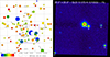 |
Fig. 2. The core of Stock 18. Left: Gaia chart for all stars (members and non-members alike) in the central 1.2′×1.2′ of Stock 18. Symbol size represents G3′ magnitude, symbol color GBP, 3 − GRP, 3, and arrows proper motion. Stars without GBP, 3 − GRP, 3 are shown without a color. The proper motions have the mean value derived for sample 1 subtracted. The purple square indicates the region shown in the right panel. Right: AstraLux z lucky image of the GLS 13 370 system, indicating the five WDS components with A divided into Aa and Ab. The intensity scale is logarithmic to show both bright and faint sources. |
2.5. Additional photometry and CHORIZOS analysis
For the stars with ALS spectroscopy we have collected their 2MASS photometry (Skrutskie et al. 2006). GLS 13 370 is unresolved in 2MASS and only partially resolved in Gaia DR3, as A has photometry in the three bands but B only in G3. We have tested that the three Gaia DR3 magnitudes are incompatible among them (in the sense of belonging to a typical extinguished O-type SED) and that it is likely that the GBP, 3 and GRP, 3 are intermediate values between those of an isolated A and a combined A,B system. Furthermore, as we will see below, there is at least a third hidden component in the system. Such a problematic Gaia DR3 photometry is not strange for a partially resolved multiple system such as GLS 13 370. For those reasons, in the procedure described in the next paragraph, we treat GLS 13 370 as unresolved with a G3′ magnitude intermediate between those of A and A,B and in the CHORIZOS analysis below we substitute the GaiaG2 + GBP, 2 + GBP, 3 + GRP, 2 + GRP, 3 bands by Tycho-2 BT + VT (Høg et al. 2000), see Maíz Apellániz & Barbá (2018) for similar examples of this procedure.
We use the SED-fitting code CHORIZOS (Maíz Apellániz 2004) to calculate the extinction properties of the stars with ALS spectroscopy. We use the SED grid of Maíz Apellániz (2013), the family of extinction laws of Maíz Apellániz et al. (2014), and the photometric calibration of Maíz Apellániz (2005a, 2006, 2007, Maíz Apellániz & Weiler (2018), Maíz Apellániz & Pantaleoni González (2018) plus the aforementioned recalibration of Gaia DR3 photometry (Weiler et al., in prep.). As shown in Maíz Apellániz & Barbá (2018) and Maíz Apellániz et al. (2021b), the family of extinction laws of Maíz Apellániz et al. (2014) provides a better fit to optical-NIR photometry of Galactic OB stars than other existing alternatives. See Maíz Apellániz (2024) for an explanation of the differences between monochromatic extinction quantities such as E(4405 − 5495) and R5495 (see appendix and Maíz Apellániz 2024) and their band-integrated equivalents such as E(B − V) and RV. For each star we fix Teff from the spectral type using the Holgado et al. (2018) scale and log d from the distance to Stock 18 determined below and we leave as free parameters the luminosity class (Maíz Apellániz 2013), a photometric equivalent to the spectroscopy luminosity class ranging from 0.0 (hypergiants) to 5.5 (ZAMS), and two extinction parameters for amount [E(4405 − 5495)] and type [R5495] of dust. As photometric information we use the nine-filter system GBP, 2 + G2 + GRP, 2 + GBP, 3 + G3 + GRP, 3 + J + H + K, except for GLS 13 370 A,B where, as already mentioned, we use Tycho-2 photometry and G3 in the optical for a total of six filters including the three 2MASS ones.
2.6. Variability information
We have cross-matched the sample in this paper with Maíz Apellániz et al. (2023) to obtain the three-band Gaia DR3 photometric dispersions of the stars with G3 < 17 mag and five-parameter astrometric solutions. The values will be used to ascertain the variability of the sample.
3. The cluster core
The left panel of Fig. 2 shows the 1.2′×1.2′ region around α = 0.400°, δ = 62.626° (or 00:01:36, +64:37:33.6). Given the relatively small number of cluster members, the exact position of the center is defined only within 2″ in RA or in declination. The value used here was determined by fitting a King profile, as explained below, and is consistent with the literature values in Table 1. The right panel of Fig. 2 shows our AstraLux image of the core centered around the GLS 13 370 system with the WDS (Mason et al. 2001) components indicated.
Figure 2 includes cluster members and non-members alike. To help differentiate between them, the represented proper motions have the mean cluster proper motion (derived later) subtracted. Most of the objects shown have small arrows, indicating that they are likely cluster members. The brightest stars have small proper motions relative to the cluster and most of the objects with large arrows are faint, as expected for a cluster-dominated population at the core. The core is rich in very red stars that correspond to a PMS population, as we will later see.
The right panel of Fig. 2 shows an excellent correspondence with the Gaia chart, as evidenced from the separations, position angles, and magnitude differences derived from our PSF fitting shown in Table 2. The most important difference is the first detection ever of a secondary component in GLS 13 370 A, which leads to its decomposition in Aa and Ab, and that is not present among the Gaia sources. Given the large magnitude difference, Ab is likely to be an intermediate-mass star that is too faint to influence the spectral classification of the Aa,Ab pair and, for that reason, we keep labelling the system as GLS 13 370 A. There are very small differences between the parameters derived from AstraLux and from Gaia in Table 2, so the influence of Ab is likely small in the Gaia position. However, GLS 13 370 A has large RUWE and parallax uncertainty σext and a somewhat anomalous proper motion in Gaia DR3, which are the likely effect of the hidden Ab component in the processing. The Δz and ΔG3′ measured are very similar for the pairs that include B, D, and E, as expected for OBA stars of similar extinction. The value is slightly more different for the Aa,C pair, where the masses are different enough for the intrinsic color difference between the two bands to become apparent.
GLS 13 370 component pairs measurements from this paper (AstraLux), Gaia DR3, and the WDS (the latest ones in that database).
4. The massive-star population of Stock 18
We show in Fig. 3 the ALS spectra for the nine stars previously mentioned and we list their spectral classifications sorted by G3′ in Table 3 and a selection of their Gaia DR3 derived properties in Table 4. Of the nine spectral types, the first seven are massive stars, GLS 22 356 is a borderline case with a mass ∼8 M⊙, and 2MASS J00012544+6437439 is likely an intermediate-mass star (but an interesting one as it is a very fast rotator, possibly the result of a merger).
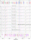 |
Fig. 3. ALS spectrograms for the nine Stock 18 stars observed with OSIRIS/GTC. |
Stars in Stock 18 with ALS spectral classifications from this paper and from the literature (Russeil et al. 2007) sorted by G3′.
Additional bright stars within 10′ of the cluster center without ALS spectral classifications.
GLS 13 370 A,B. This is the only O-type system in Stock 18 and was classified as O9 V by Mayer & Macák (1973) and as O9.5 V by Georgelin et al. (1973). We have already discussed its multiplicity above including the newly discovered Ab component. We are able to separate the A and B components in our long slit but the Aa,Ab pair is too close for its magnitude difference to be resolved (though, in principle, it should be doable with lucky spectroscopy, see Maíz Apellániz et al. 2018b, 2021c). We assigned spectral classifications of O9 V and B1: V to each component, with the uncertainty in the spectral subtype of the B component being caused by the relatively low S/N of its spectrogram. This is a likely result of spatial deconvolution noise in the extraction process. If the spectrum is extracted considering the system as a single star, the derived spectral type would be O9.2 V, a typical effect in systems with this magnitude difference. On the other hand, Ab is unlikely to be influencing the spectral classification of A enough to have shifted its subtype from O8.5 to O9 as the magnitude difference is considerably larger. Given the magnitude difference, Ab is likely to be a mid-B dwarf.
GLS 13 376 and GLS 13 368. These are the two earliest-type B stars in the cluster, both B0.5 V. The main difference between them is that the first is a moderately fast rotator, hence the (n) suffix, while the second one is a slow rotator. In addition, we point out that GLS 13368 is the farthest massive star from the center of the cluster, a factor that we analyze below.
GLS 13 362 and GLS 22 355. These two stars have the same spectral classification of B1 V yet they differ in more than one magnitude in G3′. As we will see later, the reason is the different amounts of dust in their sightlines, a consequence of the differential extinction in Stock 18.
GLS 13 365 and GLS 22 356. These two stars are classified as B1.5 V and B2 V, respectively. They are likely massive stars but close to the intermediate-mass limit.
In addition to those, we also briefly discuss other bright stars in the field. BD +63 2093 A,B is a pair of foreground stars. 2MASS J00023159+6430483 is likely a field red giant at a distance similar to that of Stock 18. 2MASS J00020363+6435079 appears to be a B star close to the distance of Stock 18 but likely in the foreground. Finally, 2MASS J00013526+6440324 is a cluster member that, given its G3′ and GBP, 3 − GRP, 3, is likely to be a B star close to the massive-intermediate mass limit.
5. Extinction analysis
The results of the CHORIZOS analysis for the stars with ALS spectral types (merging GLS 13 370 A,B, as mentioned above) are given in Table 6. The columns give, in order, the star name, the fixed parameter (Teff, the distance is also set at 2.91 kpc), the three fitted parameters, two extinction-derived parameters, MG, and the reduced χ2 (χred2) of the fit. In Figure 4 we show two examples of the fits.
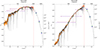 |
Fig. 4. CHORIZOS SED fits (black lines) to the observed photometry (blue error bars) for the least (left panel) and most (right panel) extinguished stars in the CHORIZOS sample. The green stars show the model SED magnitudes for each band. The orange banded region shows the Gaia DR3 XP spectrophotometry with errors but note that it is not used for the SED fits. The vertical axis spans 1.75 mag in both cases to highlight the significant differences in extinction within Stock 18. Note that both stars have the same spectral type and, hence, very similar intrinsic SEDs. |
CHORIZOS results and uncertainties, with the uncertainty for MG having a contribution added in quadrature from d = 2.91 ± 0.10 kpc.
The fits have χred2 values close to 1 or even lower, indicating that the magnitude uncertainties are correctly estimated, the filters are well calibrated, the model SEDs are a reasonable representation of the stars, and the family of extinction laws used appropriately describes the phenomenon (Maíz Apellániz & Barbá 2018; Maíz Apellániz et al. 2021b). The minor differences between the fitted SEDs and the observed XP spectrophotometry (Fig. 4, note that the spectrophotometry is not used for the fits) are caused by spectral resolution effects and systematic errors in the XP processing (Weiler et al. 2020, 2023).
In the case of GLS 13 370 A,B we excluded the K photometry from the fit, further (see above) reducing the bands used from six to five, as the magnitude in that band is inconsistent with the rest. The difference implies a K-band excess of 0.10 mag, which could be an instrumental effect (as the Aa,Ab,B system is unresolved in 2MASS) or a real physical effect. If it is the latter, it could indicate the existence of an accretion disk in the system (but no obvious Hα in emission is seen in the Gaia RP spectrophotometry and our ALS spectroscopy does not reach there) or that either Ab or B are subject to a considerably higher extinction than Aa. That does not seem to be the case for GLS 13 370 B, given its spectral type consistent with its G3′ magnitude and the similar Δm across bands for the Aa,B pair in Table 2. That leaves Ab as the possible culprit. If that were the case, Ab could be a massive star still embedded in dust, in a situation similar to the companion of Herschel 36 (Goto et al. 2006; Maíz Apellániz et al. 2015b). More data in the form of e.g. high-resolution imaging in different IR bands are needed to test that hypothesis.
With the exception of GLS 13 362, all B stars have fitted luminosity classes of 5.2–5.4, with 5.0 being a typical dwarf for that spectral type and 5.5 being a ZAMS object. This is a sign of the young age of the cluster. The higher value of GLS 13 362 indicates that it possibly contains a hidden binary component. The CHORIZOS-derived LC of ∼3.9 for GLS 13 370 A,B must be partially caused by the presence of three stars in the system but that could not be the whole story given the relatively large Δm between components. As the primary has a spectral type slightly inconsistent with that LC (and the late-O dwarf spectral classification does not show luminosity inconsistencies between He/He and Si/He criteria, see Walborn et al. 2014) and is unlikely to have progressed along an isolated evolutionary trajectory, we propose as a possibility that it is the result of a merger.
As previously detected by other authors (Table 1), there is significant differential reddening, with E(4405 − 5495) ranging from 0.55 to 0.81. Given the small uncertainties, the effect is clearly physical, as it can be also seen comparing the two panels in Fig. 4 which correspond to two stars with very similar intrinsic SEDs but quite different extinctions.
We also detect variations in R5495 within the cluster (see Maíz Apellániz & Barbá 2018 for examples in other clusters with associated H II regions) but they are smaller than those in E(4405 − 5495). Six of the eight stars are within two sigmas of R5495 = 3.38, with GLS 22 355 and GLS 13 365 being the two outliers. The average R5495 value is higher than the canonical one of 3.1, as typical of the extinction produced by dust immersed in ionized gas (Maíz Apellániz & Barbá 2018).
The uncertainties in the monochromatic extinction A5495 are smaller than those expected by the simple product of E(4405 − 5495) and R5495. This is caused by the anticorrelation between E(4405 − 5495) and R5495 described by Maíz Apellániz & Barbá (2018). The band-integrated extinction AG is always lower than the monochromatic A5495. This happens because the effective wavelength of the G3 filter is larger than 5495 Å but also due to non-linearity effects (Maíz Apellániz 2024), as the ratio of A5495 to AG increases with A5495.
6. Cluster membership and distance
6.1. Sample definitions
To select the cluster membership and calculate the distance to Stock 18 we use four primary samples (1–4) selected using the procedure described above and the criteria listed in Table 7. All samples have the same center, with the radius increasing from 4′ in sample 1–7′ in sample 2 and 10′ in sample 3 (Fig. 1). r is maintained at 10′ for sample 4 but in that case rμ is increased from 0.6 mas/a to 20 mas/a. The values listed in Table 7 were selected iteratively, as with other groups in the Villafranca project, with the idea of using sample 1 for the cluster itself based on the spatial distribution, proper motions, and extinctions of its massive stars. αc and δc were determined by fitting King profiles and minimizing the cluster radius, as detailed below. Samples 2 and 3 are spatially extended versions of sample 1 to determine the extension of a potential halo (or association) around Stock 18. Sample 4 represents the bulk of the Galactic population in Gaia DR32, as setting such a large rμ and leaving C*, Δ(GBP, 3 − GRP, 3), and RUWE only loosely constrained leave the selection algorithm to operate almost only through the normalized parallax loop. Given the Matrioshka nature of the four samples, with each subsequent one enclosing the previous samples in parameter space3, we also define differential samples X − Y as those in sample Y but not in sample X. For example, the differential sample 3–4 refers to stars in the bulk of the Galactic population excluding those within the range of proper motions of the cluster. Later on we also define a fifth sample which we call the final one.
Sample characteristics used in this paper for membership.
6.2. Sample results
The positions, magnitudes, colors, and (a selection of the) proper motions are plotted in Fig. 5, proper motion diagrams are given in Fig. 6, normalized parallax histograms are shown in Fig. 7, and CAMDs are plotted in Fig 8. A summary of the results for samples 1–4 is listed in Table 8.
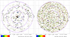 |
Fig. 5. Gaia charts for the stars in samples 1, 2, and 3 (left) and stars in differential sample 3–4 (right). The same three circles as in Fig. 1 are plotted. Symbol size represents G3′ magnitude, symbol color GBP, 3 − GRP, 3, and arrows proper motion. The magnitude and color scales are common to both panels (see legend) and stars without a valid GBP, 3 − GRP, 3 are shown without a color. The proper motions have the mean value derived for sample 1 subtracted and the two scales are different, as indicated in the legend. Only the proper motions for the 100 brightest stars in each panel are shown. |
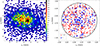 |
Fig. 6. Proper motion diagrams for different samples in this paper. Left: histogram for sample 4, excluding the regions with high relative proper motions for visibility purposes. The white circle marks the selected region for samples 1–3. Right: individual proper motions for sample 1 (blue stars) and for the differential 1–3 sample (red circles). |
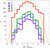 |
Fig. 7. Normalized parallax histograms for samples 1–4. The smooth curves are the expected distributions. |
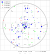 |
Fig. 8. Gaia CAMD for different samples in this paper: (top left) sample 1, (top right) differential 1–3 sample, (bottom left) differential 3–4 sample, and (bottom right) final sample. All panels include the solar metallicity Geneva-Padova 1.0 Ma MS isochrone of Maíz Apellániz (2013) and the 1.0 and 2.0 Ma PMS isochrones of Baraffe et al. (2015) with the two extinctions that span the range measured for Stock 18, E(4405 − 5495) of 0.55 and 0.81 mag, in both cases with R5495 = 3.38. Empty squares mark the initial masses in the MS isochrone and the PMS isochrones extend to 1.4 M⊙. In the first three panels each sample member is colored according to σG from Maíz Apellániz et al. (2023). In the bottom left panel typical color error bars as a function of MG are shown. In the bottom right panel the coloring scheme is the same as in Fig. 9 and reflects the probability of belonging to the cluster. A distance of 2.91 kpc is assumed for all stars (distance modulus of 12.32 mag). |
Membership and distance results for the four samples.
All four samples yield very similar distances, all within one sigma of 3.0 kpc. This indicates that the cluster is located at about the same distance (within the uncertainties) as the bulk of the Galactic population. In reality, the stars in the cluster should be located at a small range of distances of a few parsecs while the bulk of the Galactic population should extend over hundreds of parsecs. However, the external parallax uncertainties in Gaia DR3 are too large to differentiate between the two populations using parallaxes alone, especially as the bulk of the Galactic population is faint (Fig. 8) and, hence, their uncertainties are larger than for most of the bright stars in the cluster.
The normalized parallax histograms for the four samples (Fig. 7) are reasonably well approximated by Gaussians of zero mean and a dispersion of one, indicating that they are consistent with populations at a similar distance and that the external uncertainties are correctly estimated. The values of tϖ close to 1.0, as a numerical expression of the above, indicate the same. Note that the normalized parallax criterion eliminates objects with values below −3 or above +3. There are not enough stars in the first three samples for this criterion to eliminate more than maybe one member of the population, but for sample 4 it is possible that ∼10 have been removed (a small fraction of the total, in any case).
As the cluster and the bulk of the Galactic population are at similar distances, the primary means of differentiating them must be through proper motions. As shown in Table 8, samples 1–3 have similar average proper motions in the two coordinates (not unexpected given the selection criteria) while those three samples have similar average values of μδ, g when compared to sample 4 but quite different values of μα*. The effect is seen in the left panel of Fig. 6, with Stock 18 producing a significant peak in the broader proper motion distribution of sample 4. However, it is clear from that panel that sample 4 significantly contaminates at least sample 3 and quite possibly samples 1 and 2, an issue we analyze next.
6.3. Contamination and final sample definition
In order to estimate how the Galactic population at a distance similar to Stock 18 contaminates samples 1–3, we proceed along the following steps:
-
We assume that the Galactic population has a proper-motion distribution that can be described by an inclined 2-D Gaussian distribution. We fit its parameters using the left panel of Fig. 6 eliminating the white-circle region from the fit.
-
Once we have a fit, we calculate how many stars from the Galactic population are in the region inside the circle to estimate the contamination for sample 3 and then we scale those numbers proportionally to the area for samples 1 and 2 assuming a spatially uniform distribution of the contamination.
-
To estimate the probability of a star in sample 1 (or 2 or 3) of being a cluster member, we assume that the contaminants in the top panels of Fig. 8 have the same distribution in the CAMD as in the lower left panel. Each star is then assigned a probability p depending on the contaminant CAMD density in such a way that the total probability equals the expected number cleaned of contaminants.
The result of the second step is that 95 ± 12 stars in sample 1 are cluster members. There is significant contamination but ∼60% of the stars remain in the cleaned sample. The results for the differential 1–2 and 2–3 samples are very different. In the first case, almost no stars remain (6 ± 17) and in the second one only 26 ± 21 stars do: only 10% of the stars in the differential 1–3 sample are cluster members, so the vast majority of the objects beyond 4′ are just part of the Galactic population. A hint of this is seen in the right panel of Fig. 8: stars in sample 1 show a significant concentration in proper motion but stars in differential sample 1–3 show a smooth distribution. Therefore, Stock 18 is a compact cluster with a small or non-existent halo around it, an issue that is further explored below.
The result of the third step for sample 1 is shown in the bottom right panel of Fig. 8. For the final (F) sample that we employ for the IMF calculation below, we use sample 1 with four additions: (a) GLS 13 370 B (excluded from sample 1 due to its lack of GBP, 3 − GRP, 3), for which we use the existing G3′ value and estimate GBP, 3 − GRP, 3 assuming the same extinction as for A; (b) GLS 13 370 Ab (excluded from sample 1 due to its non-detection in Gaia DR3), for which we estimate G3′ from Δz and GBP, 3 − GRP, 3 from assuming the same extinction as for A; and (c) GLS 13 368 and 2MASS J00013558+6433174 (= Gaia EDR3 431 768 599 809 746 688), the two brightest blue stars in the differential 1-2 sample. They are likely to be cluster members for reasons that are explained in the next section.
7. Internal cluster dynamics and structure
7.1. Dynamical state
Now we that have a good idea of which objects are likely cluster members, we analyze the cluster dynamics and structure. In Fig. 9 we plot the positions of the stars in sample 1, using the probability color coding developed before and with the relative proper motions plotted for the 16 brightest stars. Proper motions are not plotted for fainter stars because, in general, they have larger uncertainties. In that respect, we substitute the proper motion of the high-RUWE GLS 13 370 A by that of GLS 13 370 B, as both stars are expected to form a bound system with an orbit long enough for the two proper motions to be indistinguishable within the Gaia time baseline.
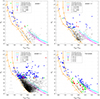 |
Fig. 9. Gaia 9′×9′ chart for sample 1 with symbol size used to represent magnitude and a coloring scheme that reflects the probability of belonging to the cluster. Arrows represent the proper motion with respect to the sample average, with the value for GLS 13 370 B substituting that of GLS 13 370 A, for the 16 brightest stars in sample 1. |
Two observations can be made about Fig. 9. First is the difference between the spatial distribution of high and low probability members. The core is clearly dominated by high-probability members while the low-probability members are dispersed throughout the field. This probability-based difference validates the decontamination procedure of the previous section. Second, the plotted relative proper motions are not randomly distributed but show a tendency towards an outward radial direction, which is an indication of an expanding motion. Furthermore, the two brightest stars in the differential sample 1–2 (see the left panel of Fig. 5, they are located in the lower part of the region, see above regarding their inclusion in the final sample) also form part of the same pattern. In order to see the effect better, in Fig. 10 we plot coordinate vs proper motion for 18 stars, the 16 brightest from sample 1 plus those two brightest from differential sample 1–2, which corresponds to objects with ≳2 M⊙. An expansion pattern is clearly seen and the inverse of the slopes of the fitted linear regressions yield dynamical (interaction-free expansion) ages of 1.06 ± 0.11 Ma in right ascension and 1.04 ± 0.06 Ma in declination, using as uncertainties the external proper motions without the systematic uncertainty (as we are only interested in the relative motions and the angular dispersion in the sky is small compared to the small-angle wavelength of ∼1° seen in the Gaia DR3 angular covariance, Maíz Apellániz et al. 2021d). The reduced χ2 values for the two fits are large (7.7 and 11.4 respectively), indicating that the expansion cannot be fully explained by a single event with no further interactions. However, the two plots in Fig. 10 treat each coordinate independently. This is just an indication of an expansion but we need to confirm it with a 2D analysis (as we cannot do a 3D analysis for lack of accurate relative distances and radial velocities), which is what we do next.
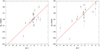 |
Fig. 10. Right ascension (left) and declination (right) coordinate vs proper motion for the 16 stars with drawn proper motions in Fig. 9 plus the two brightest stars in the differential 1–2 sample. Error bars show the external uncertainties without the systematic uncertainty, as we are dealing with relative proper motions in a small region of the sky. The red lines are the linear regression fits. |
The left panel of Fig. 11 shows the current positions of the 18 star sample. The mean (plane-of-the-sky) separation of the 153 stellar pairs is 3.28′ (2.77 pc) and the mean distance of the 18 stars to their centroid is 2.16′ (1.83 pc). We use the relative proper motions to backtrace the positions in time (assuming no gravitational interactions) and we find the time at which the mean separation is a minimum. The result is 0.61 Ma ago, when the mean pair separation was 2.35′ (1.99 pc) and the mean distance of the 18 stars to their centroid was 1.58′ (1.34 pc), with the result plotted in the center panel of Fig. 11. At that point the 18 stars clearly form a more compact configuration, as in general that panel shows empty circles (current positions) surrounding a mixture of empty and colored circles. However, the core itself appears to be not as dense as it is at the current time. This is likely a combination of two effects: the gravitational interactions at the core curving the real trajectories into orbits and the consideration that the proper motions are exact, while the reality is that they have significant external uncertainties in Gaia DR3.
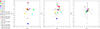 |
Fig. 11. Charts for the 18 bright stars described in the text color-coded by ID and with symbol size representing a G3′ magnitude scale. Left: Current positions. Center: Backtraced positions using the Gaia DR3 proper motions for 0.61 Ma ago, with empty circles used for the current positions and lines joining the backtraced and current positions. Right: Same as the previous panel for 0.88 Ma ago selecting the proper motions within 2.5 sigmas of the measured values that minimize the average mean separation between pairs. |
To address the uncertainty effect above we build a gradient descent Monte Carlo method to test how close the stars could have been in the past by varying the proper motions of the 18 stars. To include to some degree the effect of curvature, we allow the proper motion in each coordinate to change within 2.5 sigmas of its average (using the external uncertainties without systematic uncertainties, see above), and we search for the point in time where the mean pair separation is minimized. The result, shown in the right panel of Fig. 11 is that 0.88 Ma ago the mean separation could have been as low as 0.91′ (0.77 pc), with a corresponding mean distance of the 18 stars to their centroid of 0.61′ (0.52 pc). Furthermore, even though some of the 18 objects (e.g. 2MASS J00013558+6433174) have trajectories that only graze the compact core at a distance of a few tenths of a parsec, all of the massive stars in the system have trajectories that bring them within 0.1 pc of the core either at that age or in the range 0.8-1.1 Ma. Therefore, the data are compatible with all of the massive stars in Stock 18 being formed in an extremely compact core and being ejected within a short (∼0.3 Ma) period of time around 1 Ma ago. Currently only the GLS 13 370 Aa,Ab,B system (represented in the 18 star sample as a single object) and GLS 22 356 remain in the central 1-pc region but originally the other confirmed five massive stars could have been there as well and forming a significantly more compact system. This hypothesis may be tested with future Gaia data releases (such as DR4), as the proper motion uncertainties are expected to improve. For that purpose, we provide in Table 9 a list of the currently measured proper motions and of the ones resulting from the Monte Carlo analysis, as well as the predicted positions from 0.88 Ma ago4. If Stock 18 was indeed a very compact cluster ∼1 Ma ago, future Gaia data releases should move the proper motions from the former to something close to the latter. Given their likely origin at or near the core of Stock 18 and as already anticipated above, for the final sample used to determine the IMF below we include the two stars from the differential 1–2 sample, GLS 13 368 and 2MASS J00013558+6433174, the first a massive star with a trajectory compatible with forming part of the ∼1.0 Ma event and the second an intermediate-mass object with only a grazing trajectory with respect to the core but with a possible interaction with GLS 13 376 at a slightly later epoch.
Monte Carlo results for the proper motions and predicted positions 0.88 Ma ago for the 18 star sample.
7.2. Cluster structure
The analysis in the previous subsection was centered on the brightest stars in the cluster but, of course, the cluster is dominated in numbers by low-mass stars. To study the overall cluster structure, we fit a King profile:
 (3)
(3)
where ρ(r) is the stellar number density, fb and fc the background and cluster central number densities, and rc the cluster core radius, to sample 3 as defined above (Fig. 12). We do so by creating a histogram in the radial distribution, integrating Eq. (3) in each bin, and fitting the result using a custom-made IDL procedure. It is known that dividing data into bins can create biases in the fitted function parameters and to avoid them we adopted three complementary strategies. [a] We divided the bins in two groups, one for the core region and one for the background and in each of those groups we select bins with the same number of stars in each, as this is known to significantly reduce biases (Maíz Apellániz & Úbeda 2005). [b] After obtaining a first result, a second (final) iteration was done using as weights the values derived from the fitted function (as opposed to those derived from the data). [c] Different numbers of bins and different limits between the core and background regions were used to test for variations and to check for the validity of the uncertainties. The procedure was repeated in a 2D grid in RA+dec for the center coordinates, with the final value selected by minimizing the value of rc.
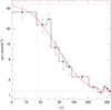 |
Fig. 12. Radial density profile for sample 3 (black) and fitted King profile (red). The dotted lines mark the fitted rc, fb, and fb+fc. |
Using sample 3, we find that the cluster center is located at αc = 0.400°, δc = 64.626°, in each case with an uncertainty of 0.001°, and those are the values we use throughout this paper (Table 7). As for the parameters of the King distribution, we obtain rc = 0.29 ± 0.08′, fc = 60 ± 24 arcmin−2, and fc = 1.2 ± 0.1 arcmin−2. Our value for the cluster core is similar to the 2MASS value derived by Bhatt et al. (2012) but lower than the rest in Table 1.
To check for possible issues with the sample selection, we repeated the procedure using different samples. First, we used the same sample 3 but with different cuts in G3 to select only low-mass stars. Second, we substitute sample 3 by the objects in the final sample with p > 0.5 (and fixing fb to a value of zero). In all cases we find similar values for the core radius, with variations much smaller than the uncertainty quoted above.
7.3. Dynamical analysis
The core radius we determine for Stock 18 of 0.24 ± 0.07 pc would be one of the smallest in the large sample of Galactic clusters of Kharchenko et al. (2013). The compact size would be remarkable by itself but it is even more so considering our discovery of the expansion of the high+intermediate mass stars from the previous subsection, which would indicate an even more compact size at birth. The outstanding question is whether the expansion detected also affects the low-mass stars. This cannot be tested directly using their proper motions at the present time, as their uncertainties in Gaia DR3 are, in general, too large. We can test it indirectly by determining the mean separation and the mean distance to their centroid for the final sample stars with p > 0.8, which should be a relatively clean sample of cluster members dominated by low-mass stars. Those values are 2.16′ and 1.66′, respectively, that is, significantly smaller that the ones for the current positions of the 18 star sample and relatively similar to the ones of that same sample 0.61 Ma ago assuming exact proper motions. Therefore, apparently the expansion of the more massive stars in Stock 18 is not shared by the stars of lower mass.
We question what mechanism could be responsible for such behavior. In the classical view of Lada & Lada (2003), most clusters go through an embedded, compact phase, after which they lose most of their associated gas and become unbound as a result. However, this does not appear to be the case for two reasons: first, because the gas appears to be cospatial with the stars and, second, because a global mass loss should affect both high- and low-mass stars equally, which does not appear to be the case for Stock 18. Indeed, a recent analysis by Miret-Roig et al. (2024) has found an average delay of 5.5 Ma between cluster formation and the onset of expansion, so it is likely too early for that to have happened. Given the very young age of Stock 18 (see below) and compactness, other mechanisms such as tidal disruption cannot be at work, either.
One process that preferentially affects massive stars are n-body interactions with n ≥ 3 (Oh et al. 2015; Oh & Kroupa 2016), since when those take place among low-mass stars alone the resulting outgoing velocities are unlikely to be above the escape velocity of the cluster. In our recent analysis of the Bermuda cluster (Villafranca O-014 NW, Maíz Apellániz et al. 2022b) we discovered how multiple stellar encounters between massive stars were able to eject so much mass in the form of high-mass systems as to provoke the expansion of the remaining low-mass stars, thus leaving and expanding cluster orphaned of massive stars. The most likely explanation for Stock 18 consistent with the data in this paper is that one or several events ∼1 Ma ago ejected some of the massive stars in the cluster but without enough mass being lost as to unbind the cluster. Therefore, this is the second cluster for which we find that dynamical interactions between massive stars have radically altered the dynamics of the system at a very early age, before gas loss is unable to contribute in a significant manner. As we pointed out in Maíz Apellániz et al. (2022b), there are hints of other clusters where this may have happened as well, such as in Villafranca O-012 S (Haffner 18) and Villafranca O-023 (Orion Nebula Cluster). One difference between Stock 18 and the other three is its lower mass, both for the cluster itself and for the most massive star. That is the likely reason for the ejected stars to have a likely low ejection velocity, thus producing only walkway stars but not runaways5.
8. Age and variability
As we mentioned in the introduction, previous age estimates indicate that Stock 18 is a very young cluster. Roger et al. (2004) analyzed the H II region to give an age of 0.25–0.50 since the activation of the main ionizing source (GLS 13 379 Aa) and Sinha et al. (2020) detected a peak in the PMS distribution at an age of 1 Ma, with some older stars. In the previous section we have obtained a dynamical age of 1 Ma with an uncertainty of just 0.1–0.2 Ma. The good agreement with the Sinha et al. (2020) points towards Stock 18 being created in such a compact state that a dynamical instability took place almost immediately. If all the massive stars were indeed inside a region as small as 0.1 pc as suggested in the previous section, the numerical simulations of Oh & Kroupa (2016) suggest that a large fraction of the massive stars may be ejected.
We can provide an independent estimate of the PMS age by analyzing the lower right panel of Fig. 8, where we have plotted the 1.0 and 2.0 Ma isochrones of Baraffe et al. (2015). As it turns out, for stars around ∼1 M⊙ differential extinction (unknown a priori for individual objects) shifts the isochrones in the CAMD in a direction nearly parallel to the isochrones themselves. This makes age relatively easy to determine and mass more difficult. For the stars with p > 0.8 we confirm the finding of Sinha et al. (2020) of a peak around an age of ∼1 Ma and we also find a handful of stars significantly younger than those. Stars with probabilities between 0.5 and 0.8 have somewhat older ages, as expected from the decontamination procedure. Therefore, our analysis confirms the young age of the PMS population.
Figure 8 and Table 4 can also be used to analyze the variability of the samples based on the values of σG from Maíz Apellániz et al. (2023). Stars in Table 4 have low variability, as expected from stars in the upper MS that are not eclipsing binaries or of Oe/Be type. There is, however, a correlation with luminosity as we go from mid-B to O stars in the MS, as seen in the large sample of Maíz Apellániz et al. (2023).
The variability analysis of Fig. 8 is limited to G3 < 17 by the input data in Maíz Apellániz et al. (2023). Most stars with σG values have low variability. The more variable stars in sample 1, with the exception of GLS 13 370 A (see above), are all intermediate-mass stars of ∼2 M⊙ at an intermediate point between the PMS and MS isochrones, that is, they are on their final stages before reaching the main sequence. As pointed out in Maíz Apellániz et al. (2023), the high σG values can be used as an approximate proxy to distinguish stars that have not yet reached the MS. Comparing that region of the CAMD with the equivalent ones for samples 1–3 and 3–4, we see that in the latter two most stars do not have high variability but a few do. Those may be the few PMS in the halo of Stock 18. In addition, those two samples also show stars further to the right (about ∼1 mag in GBP, 3 − GRP, 3) crossing in diagonal from the top left to the lower right. Those are likely red clump stars of different extinctions at a distance similar to that of Stock 18 and are also characterized by low values of σG (Maíz Apellániz et al. 2023). Finally, one star with high variability appears towards the upper right corner of the lower left panel of Fig. 8, 2MASS J00003565+6440364 and is likely a red giant.
9. IMF and cluster mass
The next step in our analysis of Stock 18 is the calculation of its IMF and total stellar mass. If extinction were (approximately) constant across the field, we could simply use the CAMD to determine the individual stellar masses using either the MS or PMS isochrones. However, as we have previously seen, there is significant differential extinction, which introduces a corresponding uncertainty in the stellar masses. This can be seen in Fig. 8, where pairs of isochrones spanning the range of extinction are shown and some initial masses are plotted in the MS isochrones for reference. As a further complication, due to the young age of the cluster, intermediate-mass stars (defined as the 1.5–8.0 M⊙ range) are in between the PMS and MS isochrones. The only case for which we can derive individual realistic stellar masses are for the objects for which we have spectral classifications.
Given that, we performed a simplified analysis by dividing our sample into three observed bins: massive stars (M > 8.0 M⊙), intermediate-mass stars (M = 1.5 − 8.0 M⊙), and low-mass stars (M = 0.7 − 1.5 M⊙), with a fourth bin of very low mass stars (M = 0.08 − 0.7 M⊙) not observed. We then counted how many stars are in each bin and compared the results with what would be expected from a canonical IMF (Kroupa 2001), see Table 10. An analysis of that table reveals:
-
All stars in the first two bins have p > 0.8.
-
If the IMF follows the canonical one for intermediate- and low-mass stars, then most of the stars with p < 0.8 are not cluster members. Slightly changing the 0.7 M⊙ value for the lowest mass observed or introducing a reasonable completeness function does not change this assessment.
-
The observed number of high-mass stars is incompatible with the expected number from a canonical IMF with 17 stars, indicating that the IMF is top-heavy.
-
If we consider the ejected stars as no longer part of the system, then the PDMF is compatible with a canonical one.
-
If we estimate the masses of the stars in the high-mass range from the CHORIZOS analysis we get a total mass that is higher by a factor of two (101 ± 4 M⊙) but a significantly lower average mass (11.3 M⊙) in comparison with the values of the canonical IMF. In other words, the IMF is top heavy but only for massive stars that are right above the 8 M⊙ limit.
-
Adopting a canonical IMF for stars with M < 8 M⊙ and the individual masses for M > 8 M⊙ we arrive to a total cluster mass of ∼300 M⊙ in the 0.08-25 M⊙ range (no stars with higher masses are present), of which 1/3 is in massive stars.
Number of stars per mass range and expected values from a canonical IMF assuming the same number of stars in the intermediate mass range.
It is interesting to compare these results with the previous ones we obtained for the Bermuda cluster in Maíz Apellániz et al. (2022b). Both are relatively low-mass clusters with a top-heavy IMF that have ejected a significant fraction of their massive stars, thus significantly reducing the cluster mass. There are differences in the IMF details (the Bermuda cluster has produced stars with higher masses, most noticeably the primary in the Bajamar system), the ejection speed (the Bermuda cluster has produced true runaways as opposed to just walkaways) and the age (the Bermuda cluster is about twice as old) but two consequences remain the same: a top-heavy IMF turns into a nearly canonical PDMF prior to any supernova explosions due to dynamical interactions and the number of free-floating compact objects in the Galaxy increases significantly. Both of those issues have important consequences for Galactic modelling, so further studies need to be pursued to establish how frequent is this phenomenon, that may have been overlooked in the past due to data of sufficient quality not being available.
10. Galactic location
The last aspect we analyze in this paper is the motion of Stock 18 with respect to the Milky Way. In Table 8 the proper motions in RA and declination of sample 1 are −2.670 ± 0.024 mas/a and −0.658 ± 0.024 mas/a, respectively. From our previous analysis of the Galactic population at the distance of Stock 18 (sample 4 discarding the proper motion region around Stock 18 and fitting a 2D Gaussian distribution) we obtain values of −2.008 ± 0.030 mas/a and −0.552 ± 0.019 mas/a. Therefore, Stock 18 has a distinct group motion with respect to the surrounding population, as the differences are many times larger than the uncertainties. Translating those values into Galactic coordinates and assuming no covariance, we obtain values of μl * ,g = −2.747 ± 0.024 mas/a and μb, g = −0.133 ± 0.024 mas/a for the cluster. The equivalent values for the Galactic population are −2.077 ± 0.030 mas/a and −0.156 ± 0.020 mas/a, respectively. At a distance of 2.91 kpc, those translate in Galactic coordinates into tangential velocities of (−37.9,−1.8) km/s and (−28.6,−2.1) km/s. Hence the cluster has a significant velocity of 9.2 km/s in the plane of the sky with respect to the surrounding population, with the vector pointing nearly parallel to the Galactic plane.
How do the group proper motions of Stock 18 and the surrounding population compare to the expected one at its Galactic location? To calculate that, we use:
-
The height of the Sun above the Galactic Plane of Maíz Apellániz et al. (2008), z⊙ = 20 pc.
-
The peculiar solar velocity with respect to the LSR of Schönrich et al. (2010): U⊙ = 11.1 km/s, V⊙ = 12.24 km/s, and W⊙ = 7.25 km/s.
-
A distance to the Galactic Center of 8.178 kpc from Abuter et al. (2019).
-
The Galactic rotation of Sofue (2020) updated in 20216.
With those parameters, we obtain −2.449 mas/a in l and −0.386 mas/a in b as the expected proper motions. At face value, with respect to the expected values in Galactic coordinates [a] Stock 18 is moving westward and the Galactic population is moving eastward and [b] both are moving northward. The difference between the Galactic population and the model in the longitude component is just 5.1 km/s, small enough that we cannot discard that the fault lies in the rotation curve model. On the other hand, the discrepancy between the cluster and the Galactic population is significant. One possible cause is the effect of the Perseus arm, where Stock 18 is located, on the motion of its natal cloud.
We also point out that at the Galactic latitude of Stock 18 of 2.27°, 2.91 kpc corresponds to a vertical distance of 115 pc, which added to the value of z⊙ yields 135 pc above the Galactic mid-plane at our location. Therefore, the cluster is located above our Galactic mid-plane and moving away from it. This is likely an effect of the Galactic warp, which in this region of the Galaxy curves upwards (Romero-Gómez et al. 2019). Indeed, the three other clusters with O stars analyzed in Villafranca I and II that are located at distances between 2 and 3 kpc and in the l = 84 − 135° region (Berkeley 90, Sh 2-158, and IC 1805) are 54–201 pc above our mid-plane, so Stock 18 is not an exception.
11. Summary and future work
A summary of the results in this paper is given in Table 11. In more detail:
-
Stock 18 is a young stellar cluster located at a distance of 2.91 ± 0.10 kpc, which in its Galactic direction corresponds to the Perseus arm.
-
It is quite compact, with a core radius of 0.24 ± 0.07 pc and no significant halo, but it was even more compact in the past. Its massive stars are expanding and currently are more disperse than its low- and intermediate-mass stars. It is possible that 0.8–1.1 Ma ago most of the massive stars were contained at one point within a space of less than 0.1 pc.
-
We propose that dynamical interactions at that time, right after cluster formation, ejected most of the massive stars. If so, this would be the second cluster in the Villafranca sample (after the Bermuda cluster) for which such interactions have produced an expansion, albeit in this case restricted to just the massive stars and with overall low-ejection velocities (i.e. walkaways instead of runaways). The process takes place before the cluster loses most of its natal gas.
-
The cluster IMF is top heavy, with 9 massive stars and only 2.7 expected from the number of intermediate-mass stars. However, if we exclude the ejected massive stars, the PDMF looks like a canonical one (or Kroupa) prior to any SN explosions. We observed this same effect in the Bermuda cluster. If confirmed for more clusters, it would have two important consequences: the true IMF would be top-heavy with respect to the canonical one, as prior calculations would have excluded the ejected stars, and the number of free-floating compact objects would be higher than expected, as the ejected stars will eventually explode as SNe.
-
The total stellar mass of Stock 18 is ∼300 M⊙, of which ∼1/3 is in massive stars.
-
There is significant differential extinction in the cluster, which hampers the derivation of some of its parameters. To a lesser degree, R5495 is also variable and, in general, larger than the canonical 3.1 value.
-
Stock 18 is above the Galactic mid-plane, likely as a result of the Galactic warp, and is moving in the plane of the sky with respect to the surrounding population at a speed of 9.2 km/s, possibly as a reflection of the motion of its natal cloud with respect to the Perseus arm.
-
The ionizing flux of the cluster is dominated by the more massive component of the GLS 13 370 system, for which we have detected for the first time a new visual component (Ab) in our AstraLux data.
Summary of results in this paper, with the fourth column referring to the relevant section/table in the paper.
The most important future line of work regarding Stock 18 will be redoing the dynamical analysis with Gaia DR4 to verify the hypothesis that the cluster was in a very compact state ∼1.0 Ma ago. We have also applied to get time to observe the core of the cluster with the WEAVE LIFU, as that would allow us to obtain spectroscopy of more stars and to derive the gas extinction from the hydrogen emission lines. We will also continue with the Villafranca project to attempt the detection of clusters in a similar state. However, we think it is unlikely that we will be able to catch a system in the act of being in a compact ∼0.1 pc state for two reasons: extinction is expected to be significantly higher at very early stages (so it would only be observable in the IR) and, if Oh & Kroupa (2016) are right, such a phase would be so unstable that it could not last long, so we would only detect systems in the aftermath.
Slowly-rotating stars have no index and increasing v sin i (or broadening the lines by other mechanism such as unresolved binarity) leads to subsequent indices of (n), n, nn, and nnn.
The bulk of the Galactic population in a given region of the sky in Gaia DR3 is at a distance determined by competing effects in two directions: on the one hand, the ever increasing volume at a given distance due to the d2 factor and, on the other hand, the dimming effect of distance and extinction that moves stars past the detection limit. Variations in stellar density can play in both directions but most frequently in the second one, especially at a Galactic latitude of more than 2° and away from the bulge such as in this case.
Such a prediction is subject to a global displacement due to the uncertainty in the subtracted cluster proper motion.
We say likely because we are not including radial velocities in our analysis.
Acknowledgments
J. M. A., A. S., and M. P. G. acknowledge support from the Spanish Government Ministerio de Ciencia e Innovación and Agencia Estatal de Investigación (10.13 039/501 100 011 033) through grant PID2022-136 640 NB-C22 and from the Consejo Superior de Investigaciones Científicas (CSIC) through grant 2022-AEP 005. The authors extend their appreciation to the Deanship of Scientific Research at Northern Border University, Arar, KSA for funding this research work through the project number “NBU-FFR-2024-237-02”. This work has made use of data from the European Space Agency (ESA) mission (Gaia, https://www.cosmos.esa.int/gaia), processed by the Gaia Data Processing and Analysis Consortium (DPAC, https://www.cosmos.esa.int/web/gaia/dpac/consortium). Funding for the DPAC has been provided by national institutions, in particular the institutions participating in the Gaia Multilateral Agreement. The Gaia data is processed with the computer resources at Mare Nostrum and the technical support provided by BSC-CNS. This work includes data obtained with the OSIRIS spectrograph at the 10.4 m Gran Telescopio de Canarias (GTC) and with the AstraLux lucky imaging instrument at the 2.2 m Telescope at Calar Alto (CAHA).
References
- Abuter, R., Amorim, A., Bauböck, M., et al. 2019, A&A, 625, L10 [NASA ADS] [CrossRef] [EDP Sciences] [Google Scholar]
- Ansín, T., Gamen, R., Morrell, N. I., et al. 2023, MNRAS, 525, 4566 [CrossRef] [Google Scholar]
- Baraffe, I., Homeier, D., Allard, F., & Chabrier, G. 2015, A&A, 577, A42 [NASA ADS] [CrossRef] [EDP Sciences] [Google Scholar]
- Bhatt, H., Sagar, R., & Pandey, J. 2012, New Astron., 17, 160 [NASA ADS] [CrossRef] [Google Scholar]
- Brown, A. G., Vallenari, A., Prusti, T., et al. 2021, A&A, 649, A1 [NASA ADS] [CrossRef] [EDP Sciences] [Google Scholar]
- Buckner, A. S. M., & Froebrich, D. 2013, MNRAS, 436, 1465 [NASA ADS] [CrossRef] [Google Scholar]
- Bukowiecki, Ł., Maciejewski, G., Konorski, P., & Strobel, A. 2011, Act Astron., 61, 231 [Google Scholar]
- Cantat-Gaudin, T., & Anders, F. 2020, A&A, 633, A99 [NASA ADS] [CrossRef] [EDP Sciences] [Google Scholar]
- Cantat-Gaudin, T., & Brandt, T. D. 2021, A&A, 649, A124 [NASA ADS] [CrossRef] [EDP Sciences] [Google Scholar]
- Cantat-Gaudin, T., Anders, F., Castro-Ginard, A., et al. 2020, A&A, 640, A1 [NASA ADS] [CrossRef] [EDP Sciences] [Google Scholar]
- Dias, W., Monteiro, H., Caetano, T., et al. 2014, A&A, 564, A79 [NASA ADS] [CrossRef] [EDP Sciences] [Google Scholar]
- Fabricius, C., Luri, X., Arenou, F., et al. 2021, A&A, 649, A5 [NASA ADS] [CrossRef] [EDP Sciences] [Google Scholar]
- Georgelin, Y. M., Georgelin, Y. P., & Roux, S. 1973, A&A, 25, 337 [NASA ADS] [Google Scholar]
- Gilmore, G., Randich, S., Asplund, M., et al. 2012, The Messenger, 147, 25 [NASA ADS] [Google Scholar]
- Goto, M., Stecklum, B., Linz, H., et al. 2006, ApJ, 649, 299 [CrossRef] [Google Scholar]
- Høg, E., Fabricius, C., Makarov, V. V., et al. 2000, A&A, 355, L27 [Google Scholar]
- Holgado, G., Simón-Díaz, S., Barbá, R. H., et al. 2018, A&A, 613, A65 [NASA ADS] [CrossRef] [EDP Sciences] [Google Scholar]
- Joshi, Y. C., Dambis, A., Pandey, A. K., & Joshi, S. 2016, A&A, 593, A116 [NASA ADS] [CrossRef] [EDP Sciences] [Google Scholar]
- Kharchenko, N., Piskunov, A., Schilbach, E., Röser, S., & Scholz, R.-D. 2013, A&A, 558, A53 [NASA ADS] [CrossRef] [EDP Sciences] [Google Scholar]
- Kroupa, P. 2001, MNRAS, 322, 231 [NASA ADS] [CrossRef] [Google Scholar]
- Lada, C. J., & Lada, E. A. 2003, ARA&A, 41, 57 [Google Scholar]
- Lindegren, L., Hernández, J., Bombrun, A., et al. 2018a, A&A, 616, A2 [NASA ADS] [CrossRef] [EDP Sciences] [Google Scholar]
- Lindegren, L., Hernández, J., Bombrun, A., et al. 2018b, Gaia DR2 astrometry, http://www.cosmos.esa.int/documents/29201/1770596/Lindegren_GaiaDR2_Astrometry_extended.pdf [Google Scholar]
- Lindegren, L., Klioner, S., Hernández, J., et al. 2021, A&A, 649, A2 [NASA ADS] [CrossRef] [EDP Sciences] [Google Scholar]
- MacConnell, D. 2006, Dyn. Astron. Latin Am., 25, 73 [NASA ADS] [Google Scholar]
- Maíz Apellániz, J. 2001, AJ, 121, 2737 [Google Scholar]
- Maíz Apellániz, J. 2004, PASP, 116, 859 [Google Scholar]
- Maíz Apellániz, J. 2005a, PASP, 117, 615 [CrossRef] [Google Scholar]
- Maíz Apellániz, J. 2005b, ESA Special Publ., 576, 179 [Google Scholar]
- Maíz Apellániz, J. 2006, AJ, 131, 1184 [CrossRef] [Google Scholar]
- Maíz Apellániz, J. 2007, ASP Conf. Ser., 364, 227 [Google Scholar]
- Maíz Apellániz, J. 2010, A&A, 518, A1 [NASA ADS] [CrossRef] [EDP Sciences] [Google Scholar]
- Maíz Apellániz, J. 2013, Highlights of Spanish Astrophysics, VII, 657 [Google Scholar]
- Maíz Apellániz, J. 2019, A&A, 630, A119 [NASA ADS] [CrossRef] [EDP Sciences] [Google Scholar]
- Maíz Apellániz, J. 2022, A&A, 657, A130 [NASA ADS] [CrossRef] [EDP Sciences] [Google Scholar]
- Maíz Apellániz, J. 2024, ArXiv e-prints [arXiv:2401.01116] [Google Scholar]
- Maíz Apellániz, J., & Barbá, R. H. 2018, A&A, 613, A9 [Google Scholar]
- Maíz Apellániz, J., & Pantaleoni González, M. 2018, A&A, 616, L7 [NASA ADS] [CrossRef] [EDP Sciences] [Google Scholar]
- Maíz Apellániz, J., & Úbeda, L. 2005, ApJ, 629, 873 [CrossRef] [Google Scholar]
- Maíz Apellániz, J., & Weiler, M. 2018, A&A, 619, A180 [Google Scholar]
- Maíz Apellániz, J., Walborn, N. R., Galué, H. Á., & Wei, L. H. 2004, ApJS, 151, 103 [CrossRef] [Google Scholar]
- Maíz Apellániz, J., Alfaro, E. J., & Sota, A. 2008, ArXiv e-prints [arXiv:0804.2553] [Google Scholar]
- Maíz Apellániz, J., Sota, A., Walborn, N. R., et al. 2011, HSA, 6, 467 [Google Scholar]
- Maíz Apellániz, J., Pellerin, A., Barbá, R. H., et al. 2012, ASP Conf. Ser., 465, 484 [NASA ADS] [Google Scholar]
- Maíz Apellániz, J., Evans, C. J., Barbá, R. H., et al. 2014, A&A, 564, A63 [CrossRef] [EDP Sciences] [Google Scholar]
- Maíz Apellániz, J., Alfaro, E. J., Arias, J. I., et al. 2015a, HSA, 8, 603 [Google Scholar]
- Maíz Apellániz, J., Úbeda, L., Barbá, R.-H., et al. 2015b, HSA, 8, 604 [Google Scholar]
- Maíz Apellániz, J., Sota, A., Arias, J. I., et al. 2016, ApJS, 224, 4 [CrossRef] [Google Scholar]
- Maíz Apellániz, J., Barbá, R. H., Simón-Díaz, S., et al. 2018a, A&A, 615, A161 [NASA ADS] [CrossRef] [EDP Sciences] [Google Scholar]
- Maíz Apellániz, J., Pantaleoni González, M., Barbá, R. H., et al. 2018b, A&A, 616, A149 [NASA ADS] [CrossRef] [EDP Sciences] [Google Scholar]
- Maíz Apellániz, J., Trigueros Páez, E., Jiménez Martínez, I., et al. 2019a, HSA, 10, 420 [Google Scholar]
- Maíz Apellániz, J., Trigueros Páez, E., Negueruela, I., et al. 2019b, A&A, 626, A20 [NASA ADS] [CrossRef] [EDP Sciences] [Google Scholar]
- Maíz Apellániz, J., Crespo Bellido, P., Barbá, R. H., Fernández Aranda, R., & Sota, A. 2020, A&A, 643, A138 [NASA ADS] [CrossRef] [EDP Sciences] [Google Scholar]
- Maíz Apellániz, J., Alfaro, E. J., Barbá, R. H., et al. 2021a, MNRAS, 506, 3138 [CrossRef] [Google Scholar]
- Maíz Apellániz, J., Barbá, R. H., Caballero, J. A., Bohlin, R. C., & Fariña, C. 2021b, MNRAS, 501, 2487 [CrossRef] [Google Scholar]
- Maíz Apellániz, J., Barbá, R. H., Fariña, C., et al. 2021c, A&A, 646, A11 [NASA ADS] [CrossRef] [EDP Sciences] [Google Scholar]
- Maíz Apellániz, J., Pantaleoni González, M., & Barbá, R. H. 2021d, A&A, 649, A13 [NASA ADS] [CrossRef] [EDP Sciences] [Google Scholar]
- Maíz Apellániz, J., Barbá, R. H., Fernández Aranda, R., et al. 2022a, A&A, 657, A131 [NASA ADS] [CrossRef] [EDP Sciences] [Google Scholar]
- Maíz Apellániz, J., Pantaleoni González, M., Barbá, R. H., & Weiler, M. 2022b, A&A, 657, A72 [NASA ADS] [CrossRef] [EDP Sciences] [Google Scholar]
- Maíz Apellániz, J., Holgado, G., Pantaleoni González, M., & Caballero, J. A. 2023, A&A, 677, A137 [NASA ADS] [CrossRef] [EDP Sciences] [Google Scholar]
- Mason, B. D., Wycoff, G. L., Hartkopf, W. I., Douglass, G. G., & Worley, C. E. 2001, AJ, 122, 3466 [Google Scholar]
- Mayer, P., & Macák, P. 1973, Bull. Astron. Inst. Czechoslovakia, 24, 50 [NASA ADS] [Google Scholar]
- Miret-Roig, N., Alves, J., Barrado, D., et al. 2024, Nat. Astron., 8, 216 [Google Scholar]
- Negueruela, I., Alfaro, E. J., Dorda, R., et al. 2022, A&A, 664, A146 [NASA ADS] [CrossRef] [EDP Sciences] [Google Scholar]
- Netopil, M., Paunzen, E., & Carraro, G. 2015, A&A, 582, A19 [NASA ADS] [CrossRef] [EDP Sciences] [Google Scholar]
- Oh, S., & Kroupa, P. 2016, A&A, 590, A107 [NASA ADS] [CrossRef] [EDP Sciences] [Google Scholar]
- Oh, S., Kroupa, P., & Pflamm-Altenburg, J. 2015, ApJ, 805, 92 [Google Scholar]
- Pantaleoni González, M., Maíz Apellániz, J., Barbá, R. H., & Reed, B. C. 2021, MNRAS, 504, 2968 [CrossRef] [Google Scholar]
- Putkuri, C., Gamen, R., Morrell, N. I., et al. 2023, MNRAS, 525, 6084 [NASA ADS] [CrossRef] [Google Scholar]
- Reed, B. C. 2003, AJ, 125, 2531 [NASA ADS] [CrossRef] [Google Scholar]
- Riello, M., De Angeli, F., Evans, D. W., et al. 2018, A&A, 616, A3 [NASA ADS] [CrossRef] [EDP Sciences] [Google Scholar]
- Riello, M., De Angeli, F., Evans, D. W., et al. 2021, A&A, 649, A3 [NASA ADS] [CrossRef] [EDP Sciences] [Google Scholar]
- Roger, R., McCutcheon, W., Purton, C., & Dewdney, P. 2004, A&A, 425, 553 [NASA ADS] [CrossRef] [EDP Sciences] [Google Scholar]
- Romero-Gómez, M., Mateu, C., Aguilar, L., Figueras, F., & Castro-Ginard, A. 2019, A&A, 627, A150 [NASA ADS] [CrossRef] [EDP Sciences] [Google Scholar]
- Russeil, D., Adami, C., & Georgelin, Y. 2007, A&A, 470, 161 [NASA ADS] [CrossRef] [EDP Sciences] [Google Scholar]
- Sampedro, L., Dias, W., Alfaro, E. J., Monteiro, H., & Molino, A. 2017, MNRAS, 470, 3937 [NASA ADS] [CrossRef] [Google Scholar]
- Schönrich, R., Binney, J., & Dehnen, W. 2010, MNRAS, 403, 1829 [NASA ADS] [CrossRef] [Google Scholar]
- Sharpless, S. 1959, ApJS, 4, 257 [Google Scholar]
- Simón-Díaz, S., Caballero, J. A., Lorenzo, J., et al. 2015, ApJ, 799, 169 [CrossRef] [Google Scholar]
- Sinha, T., Sharma, S., Pandey, A., et al. 2020, MNRAS, 493, 267 [NASA ADS] [CrossRef] [Google Scholar]
- Skrutskie, M., Cutri, R., Stiening, R., et al. 2006, ApJ, 131, 1163 [CrossRef] [Google Scholar]
- Sofue, Y. 2020, Galaxies, 8, 37 [Google Scholar]
- Vallenari, A., Brown, A., Prusti, T., et al. 2023, A&A, 674, A1 [NASA ADS] [CrossRef] [EDP Sciences] [Google Scholar]
- Walborn, N. R., Sana, H., Simón-Díaz, S., et al. 2014, A&A, 564, A40 [NASA ADS] [CrossRef] [EDP Sciences] [Google Scholar]
- Weiler, M., Carrasco, J. M., Fabricius, C., & Jordi, C. 2020, A&A, 637, A85 [NASA ADS] [CrossRef] [EDP Sciences] [Google Scholar]
- Weiler, M., Carrasco, J. M., Fabricius, C., & Jordi, C. 2023, A&A, 671, A52 [NASA ADS] [CrossRef] [EDP Sciences] [Google Scholar]
Appendix A: Glossary
We provide a list of acronyms and terms used in this paper.
-
αc, δc: Filtering central coordinates for cluster membership selection (cluster center), see Villafranca papers.
-
ALS: Alma Luminous Star.
-
A5495: Monochromatic extinction at 5495 Å, see Maíz Apellániz (2024).
-
AG: Extinction integrated over the G3 band.
-
ALS: Alma Luminous Star catalog, Reed (2003), Pantaleoni González et al. (2021).
-
C*: Photometric contamination parameter from Eqn. 6 of Riello et al. (2021).
-
CAMD: Color-Absolute Magnitude Diagram.
-
CCD: Charged-Coupled Device.
-
CDS: Centre de Données astronomiques de Strasbourg.
-
CHORIZOS: a CHi-square cOde for parameteRized modelIng and characteriZation of phOtometry and Spectrophotometry, Maíz Apellániz (2004).
-
CMD: Color-Magnitude Diagram.
-
CSIC: Consejo Superior de Investigaciones Científicas.
-
d: Group distance.
-
Δ(GBP, 3 − GRP, 3): Filtering color displacement with respect to isochrone, see Villafranca papers.
-
Δm: Magnitude difference in a binary system.
-
E(4405 − 5495): Monochromatic color excess between 4405 Å and 5495 Å, see Maíz Apellániz (2024).
-
ESA: European Space Agency.
-
fc: Central source density for the King profile.
-
fb: Background source density for the King profile.
-
G2: Gaia DR2 G-band magnitude.
-
G3: Gaia EDR3 G-band magnitude.
-
G2′: Gaia DR2 corrected G-band magnitude (Weiler et al. in prep.).
-
G3′: Gaia EDR3 corrected G-band magnitude (Weiler et al. in prep.).
-
GBP, 2: Gaia DR2 BP-band magnitude.
-
GBP, 3: Gaia EDR3 BP-band magnitude.
-
GRP, 2: Gaia DR2 RP-band magnitude.
-
GRP, 3: Gaia EDR3 RP-band magnitude.
-
GBP, 3 − GRP, 3: Gaia EDR3 BP−RP color.
-
Gaia DR2: Second Gaia Data Release.
-
Gaia EDR3: Early third Gaia Data Release.
-
Gaia DR3: Third Gaia Data Release.
-
Gaia DR4: Fourth Gaia Data Release.
-
GLS: Galactic Luminous Star.
-
GOSC: Galactic O-Star Catalog, Maíz Apellániz et al. (2004).
-
GOSSS: Galactic O-Star Spectroscopic Survey, Maíz Apellániz et al. (2011).
-
GTC: Gran Telescopio de Canarias.
-
HRD: Hertzsprung-Russell Diagram.
-
IMF: Initial mass Function.
-
k: Multiplicative constant for parallax/proper motion uncertainties, see Maíz Apellániz (2022) and Eqn. 2.
-
LC: Luminosity class, either from spectral classification or as fitted by CHORIZOS.
-
LiLiMaRlin: Library of Libraries of Massive-Star High-Resolution Spectra, Maíz Apellániz et al. (2019a).
-
LLS: LMC Luminous Star.
-
LMC: Large Magellanic Cloud.
-
LSR: Local Standard of Rest.
-
μα * ,c, μδ, c: Filtering central proper motion for cluster membership selection, see Villafranca papers.
-
μα * ,g, μδ, g: Group proper motion in equatorial coordinates, see Villafranca papers.
-
μl * ,g, μb, g: Group proper motion in Galactic coordinates, see the Gaia https://gea.esac.esa.int/archive/documentation/GDR2/Dataprocessing/chapcu3ast/seccu3astintro/sseccu3astintrotansforms.html7.
-
MG: Absolute magnitude in the G3 band.
-
MGB: Marxist Ghost Buster, Maíz Apellániz et al. (2012); Maíz Apellániz et al. (2015a).
-
MS: Main Sequence.
-
MW: Milky Way.
-
N*, 0: Number of stars in group before normalized parallax filtering, see Villafranca papers.
-
N*: Number of stars in group after normalized parallax filtering, see Villafranca papers.
-
p: Cluster membership probability.
-
ϖ: Individual Gaia (E)DR3 parallax.
-
ϖc: Individual corrected Gaia (E)DR3 parallax, see Eqn. 1.
-
ϖg: Group parallax, see Villafranca papers.
-
PA: Position angle in a binary system (secondary with respect to primary) from N towards E.
-
PDMF: Present Day Mass Function.
-
PMS: Pre-main sequence.
-
r: Filtering separation from the center in the plane of the sky, see Villafranca papers.
-
rc: Core radius for the King profile.
-
rμ: Filtering separation from the center in proper motion, see Villafranca papers.
-
R5495: Ratio of monochromatic extinction to color excess, see Maíz Apellániz (2024).
-
RUWE: Renormalized Unit Weight Error.
-
ρ(r): Stellar number density.
-
σint: Individual Gaia (E)DR3 parallax/proper motion uncertainty, see Eqn. 2.
-
σext: Individual Gaia (E)DR3 corrected parallax/proper motion uncertainty, see Eqn. 2.
-
σs: Gaia (E)DR3 parallax/proper motion systematic uncertainty, see Maíz Apellániz et al. (2021d) and Eqn. 2.
-
σϖg: Group parallax uncertainty, see Villafranca papers.
-
σX: Astrophysical photometric dispersion for band X (G3, GBP, 3, or GRP, 3) from Maíz Apellániz et al. (2023).
-
SB1: Single-lined spectroscopic binary.
-
SB2: Double-lined spectroscopic binary.
-
SED: Spectral Energy Distribution.
-
SLS: SMC Luminous Star.
-
SMC: Small Magellanic Cloud.
-
SN: Supernova.
-
tϖ: Normalized χ2 test for the group parallax, see Villafranca papers.
-
tμα*: Normalized χ2 test for the group proper motion in α, see Villafranca papers.
-
tμδ: Normalized χ2 test for the group proper motion in δ, see Villafranca papers.
-
U⊙, V⊙, W⊙: Components of the peculiar solar velocity with respect to the LSR.
-
χred2: Reduced χ2 of the CHORIZOS fit.
-
WDS: Washington Double Star catalog, Mason et al. (2001).
-
z⊙: Height of the Sun above the Galactic Plane.
-
ZP: Parallax zero point, see Eqn. 1.
All Tables
GLS 13 370 component pairs measurements from this paper (AstraLux), Gaia DR3, and the WDS (the latest ones in that database).
Stars in Stock 18 with ALS spectral classifications from this paper and from the literature (Russeil et al. 2007) sorted by G3′.
Additional bright stars within 10′ of the cluster center without ALS spectral classifications.
CHORIZOS results and uncertainties, with the uncertainty for MG having a contribution added in quadrature from d = 2.91 ± 0.10 kpc.
Monte Carlo results for the proper motions and predicted positions 0.88 Ma ago for the 18 star sample.
Number of stars per mass range and expected values from a canonical IMF assuming the same number of stars in the intermediate mass range.
Summary of results in this paper, with the fourth column referring to the relevant section/table in the paper.
All Figures
|
Fig. 1. Images of Stock 18. Left: three-channel DSS2 RGB image with the red channel corresponding to the NIR survey, the green channel to the Red survey, and the blue channel to the Blue survey. Right: WISE RGB image with the red channel corresponding to the W4 band, the green channel to a sum of the W3 and W2 bands, and the blue channel to the W1 band. In both cases, the intensity scale is logarithmic and circles with radii of 4′, 7′, and 10′ centered on the cluster are plotted |
| In the text | |
|
Fig. 2. The core of Stock 18. Left: Gaia chart for all stars (members and non-members alike) in the central 1.2′×1.2′ of Stock 18. Symbol size represents G3′ magnitude, symbol color GBP, 3 − GRP, 3, and arrows proper motion. Stars without GBP, 3 − GRP, 3 are shown without a color. The proper motions have the mean value derived for sample 1 subtracted. The purple square indicates the region shown in the right panel. Right: AstraLux z lucky image of the GLS 13 370 system, indicating the five WDS components with A divided into Aa and Ab. The intensity scale is logarithmic to show both bright and faint sources. |
| In the text | |
|
Fig. 3. ALS spectrograms for the nine Stock 18 stars observed with OSIRIS/GTC. |
| In the text | |
|
Fig. 4. CHORIZOS SED fits (black lines) to the observed photometry (blue error bars) for the least (left panel) and most (right panel) extinguished stars in the CHORIZOS sample. The green stars show the model SED magnitudes for each band. The orange banded region shows the Gaia DR3 XP spectrophotometry with errors but note that it is not used for the SED fits. The vertical axis spans 1.75 mag in both cases to highlight the significant differences in extinction within Stock 18. Note that both stars have the same spectral type and, hence, very similar intrinsic SEDs. |
| In the text | |
|
Fig. 5. Gaia charts for the stars in samples 1, 2, and 3 (left) and stars in differential sample 3–4 (right). The same three circles as in Fig. 1 are plotted. Symbol size represents G3′ magnitude, symbol color GBP, 3 − GRP, 3, and arrows proper motion. The magnitude and color scales are common to both panels (see legend) and stars without a valid GBP, 3 − GRP, 3 are shown without a color. The proper motions have the mean value derived for sample 1 subtracted and the two scales are different, as indicated in the legend. Only the proper motions for the 100 brightest stars in each panel are shown. |
| In the text | |
|
Fig. 6. Proper motion diagrams for different samples in this paper. Left: histogram for sample 4, excluding the regions with high relative proper motions for visibility purposes. The white circle marks the selected region for samples 1–3. Right: individual proper motions for sample 1 (blue stars) and for the differential 1–3 sample (red circles). |
| In the text | |
|
Fig. 7. Normalized parallax histograms for samples 1–4. The smooth curves are the expected distributions. |
| In the text | |
|
Fig. 8. Gaia CAMD for different samples in this paper: (top left) sample 1, (top right) differential 1–3 sample, (bottom left) differential 3–4 sample, and (bottom right) final sample. All panels include the solar metallicity Geneva-Padova 1.0 Ma MS isochrone of Maíz Apellániz (2013) and the 1.0 and 2.0 Ma PMS isochrones of Baraffe et al. (2015) with the two extinctions that span the range measured for Stock 18, E(4405 − 5495) of 0.55 and 0.81 mag, in both cases with R5495 = 3.38. Empty squares mark the initial masses in the MS isochrone and the PMS isochrones extend to 1.4 M⊙. In the first three panels each sample member is colored according to σG from Maíz Apellániz et al. (2023). In the bottom left panel typical color error bars as a function of MG are shown. In the bottom right panel the coloring scheme is the same as in Fig. 9 and reflects the probability of belonging to the cluster. A distance of 2.91 kpc is assumed for all stars (distance modulus of 12.32 mag). |
| In the text | |
|
Fig. 9. Gaia 9′×9′ chart for sample 1 with symbol size used to represent magnitude and a coloring scheme that reflects the probability of belonging to the cluster. Arrows represent the proper motion with respect to the sample average, with the value for GLS 13 370 B substituting that of GLS 13 370 A, for the 16 brightest stars in sample 1. |
| In the text | |
|
Fig. 10. Right ascension (left) and declination (right) coordinate vs proper motion for the 16 stars with drawn proper motions in Fig. 9 plus the two brightest stars in the differential 1–2 sample. Error bars show the external uncertainties without the systematic uncertainty, as we are dealing with relative proper motions in a small region of the sky. The red lines are the linear regression fits. |
| In the text | |
|
Fig. 11. Charts for the 18 bright stars described in the text color-coded by ID and with symbol size representing a G3′ magnitude scale. Left: Current positions. Center: Backtraced positions using the Gaia DR3 proper motions for 0.61 Ma ago, with empty circles used for the current positions and lines joining the backtraced and current positions. Right: Same as the previous panel for 0.88 Ma ago selecting the proper motions within 2.5 sigmas of the measured values that minimize the average mean separation between pairs. |
| In the text | |
|
Fig. 12. Radial density profile for sample 3 (black) and fitted King profile (red). The dotted lines mark the fitted rc, fb, and fb+fc. |
| In the text | |
Current usage metrics show cumulative count of Article Views (full-text article views including HTML views, PDF and ePub downloads, according to the available data) and Abstracts Views on Vision4Press platform.
Data correspond to usage on the plateform after 2015. The current usage metrics is available 48-96 hours after online publication and is updated daily on week days.
Initial download of the metrics may take a while.