| Issue |
A&A
Volume 671, March 2023
|
|
|---|---|---|
| Article Number | A20 | |
| Number of page(s) | 50 | |
| Section | Galactic structure, stellar clusters and populations | |
| DOI | https://doi.org/10.1051/0004-6361/202245335 | |
| Published online | 01 March 2023 | |
Gaia-ESO survey: Massive stars in the Carina Nebula
I. A new census of OB stars⋆
1
Departamento de Física Aplicada, Universidad de Alicante, 03690 San Vicente del Raspeig, Alicante, Spain
e-mail: This email address is being protected from spambots. You need JavaScript enabled to view it.
2
Astrophysics Group, Keele University, Keele, ST5 5BG Staffordshire, UK
3
Centro de Astrobiología (CAB), CSIC-INTA, Campus ESAC, 28692 Villanueva de la Cañada, Madrid, Spain
4
Instituto de Astrofísica de Canarias, 38200 La Laguna, Tenerife, Spain
5
Departamento de Astrofísica, Universidad de La Laguna, 38205 La Laguna, Tenerife, Spain
6
Royal Observatory of Belgium, Ringlaan 3, 1180 Brussels, Belgium
7
School of Architecture, Universidad Europea de Canarias, Tenerife, Spain
8
ESO, Karl-Schwarzschild-Strasse 2, 85748 Garching bei München, Germany
9
Space Sciences, Technologies and Astrophysics Research (STAR) Institute, Université de Liège, Allée du 6 Août, 19c Bât B5c, 4000 Liège, Belgium
10
Departamento de Astrofísica y Física de la Atmósfera, Universidad Complutense de Madrid, 28040 Madrid, Spain
11
Instituto de Astronomía y Física del Espacio, UBA-CONICET. CC 67, Suc. 28, 1428 Buenos Aires, Argentina
12
Instituto de Astrofísica de Andalucía (IAA), CSIC, Glorieta de la Astronomía s/n, 18008 Granada, Spain
13
Max Planck Institute for Astronomy, Königstuhl 17, 69117 Heidelberg, Germany
14
Niels Bohr International Academy, Niels Bohr Institute, University of Copenhagen, Blegdamsvej 17, 2100 Copenhagen, Denmark
15
Dipartimento di Fisica e Astronomia Galileo Galilei, Universitá di Padova, Vicolo Osservatorio 3, 35122 Padova, Italy
16
Department of Physics & Astronomy, University College London, Gower Street, London WC1E 6BT, UK
17
INAF – Osservatorio Astrofisico di Arcetri, Largo E. Fermi 5, 50125 Florence, Italy
18
Armagh Observatory and Planetarium, College Hill, Armagh BT61 9DG, UK
Received:
31
October
2022
Accepted:
18
January
2023
Abstract
Context. The Carina Nebula is one of the major massive star-forming regions in the Galaxy. Its relatively nearby distance (2.35 kpc) makes it an ideal laboratory for the study of massive star formation, structure, and evolution, both for individual stars and stellar systems. Thanks to the high-quality spectra provided by the Gaia-ESO survey and the LiLiMaRlin library, as well as Gaia EDR3 astrometry, a detailed and homogeneous spectroscopic characterization of its massive stellar content can be carried out.
Aims. Our main objective is to spectroscopically characterize all massive members of the Carina Nebula in the Gaia-ESO survey footprint to provide an updated census of massive stars in the region and an updated estimate of the binary fraction of O stars.
Methods. We performed accurate spectral classification using an interactive code that compares spectra with spectral libraries of OB standard stars, as well as line-based classic methods. We calculated membership using our own algorithm based on Gaia EDR3 astrometry. To check the correlation between the spectroscopic n-qualifier and the rotational velocity, we used a semi-automated tool for the line-broadening characterization of OB stars based on a combined Fourier transform and goodness-of-fit methodology.
Results. The Gaia-ESO survey sample of massive OB stars in the Carina Nebula consists of 234 stars. The addition of brighter sources from the Galactic O-Star Spectroscopic Survey and additional sources from the literature allows us to create the most complete census of massive OB stars so far in the region. It contains a total of 316 stars, with 18 of them in the background and 4 in the foreground. Of the 294 stellar systems in Car OB1, 74 are of O type, 214 are of nonsupergiant B type, and 6 are of WR or nonO supergiant (II to Ia) spectral class. We identify 20 spectroscopic binary systems with an O-star primary, of which 6 are reported for the first time, and another 18 with a B-star primary, of which 13 are new detections. The average observed double-lined binary fraction of O-type stars in the surveyed region is 0.35, which represents a lower limit. We find a good correlation between the spectroscopic n-qualifier and the projected rotational velocity of the stars. The fraction of candidate runaways among the stars with and without the n-qualifier is 4.4% and 2.4%, respectively, although nonresolved double-lined binaries could be contaminating the sample of fast rotators.
Key words: stars: massive / stars: early-type / stars: rotation / proper motions / binaries: spectroscopic / open clusters and associations: individual: Carina Nebula
Tables A.1 and A.2 are only available at the CDS via anonymous ftp to cdsarc.cds.unistra.fr (130.79.128.5) or via https://cdsarc.cds.unistra.fr/viz-bin/cat/J/A+A/671/A20
© The Authors 2023
 Open Access article, published by EDP Sciences, under the terms of the Creative Commons Attribution License (https://creativecommons.org/licenses/by/4.0), which permits unrestricted use, distribution, and reproduction in any medium, provided the original work is properly cited.
This article is published in open access under the Subscribe to Open model. This email address is being protected from spambots. You need JavaScript enabled to view it. to support open access publication.
1. Introduction
The Gaia-ESO Large Public Spectroscopic Survey (GES; Gilmore et al. 2022; Randich et al. 2022) has obtained high-quality spectra for ∼105 stars in our Galaxy using FLAMES at the Very Large Telescope (VLT) with its high-resolution UVES and its intermediate-resolution GIRAFFE spectrographs. GES has systematically covered all the major components of the Milky Way, providing a homogeneous and unique overview of the kinematics, chemical composition, formation history, and evolution of young, mature, and ancient Galactic populations. Open clusters are useful tools for this aim, where it is possible to study stellar populations of different ages in different evolutionary stages (see Bragaglia et al. 2022).
Numerous spectroscopic studies have been carried out on massive stars in Galactic young stellar clusters and OB associations, the most extensive to date being the Galactic O-Star Spectroscopic Survey (GOSSS; Maíz Apellániz et al. 2011). As some examples of such studies, Figer (2005) determined the upper mass limit of the initial mass function (IMF) in the Arches Cluster, a result that was later challenged by studies in R136 (Crowther et al. 2010). Other examples are the determination of the chemical composition of stars in Orion (Simón-Díaz 2010); the membership, chemical and stellar parameter determination studies in Cygnus OB2 (Berlanas et al. 2018a,b, 2020); the characterization of very massive obscured clusters in the Milky Way such as Westerlund 1 (Clark et al. 2005; Negueruela et al. 2010, 2022); and the analysis of the multiplicity of massive stars in clusters (De Becker et al. 2004, 2006; Mahy et al. 2009, 2013; Sana & Evans 2011; Banyard et al. 2023) and in the whole northern hemisphere (Maíz Apellániz et al. 2019b; Trigueros Páez et al. 2021; Mahy et al. 2022). Outside the Milky Way, the most thorough spectroscopic analysis is that of the many papers1 published by the VLT-FLAMES Tarantula Survey collaboration (VFTS, Evans et al. 2011).
The Carina Nebula complex consists of several stellar groups, some bound and some not, immersed in the Car OB1 association (Maíz Apellániz et al. 2020, 2022a; hereafter referred to as Villafranca I and II, respectively, and references therein). This complex represents a unique region for studying Galactic massive stars with FLAMES as it contains a large number of O-type stars (Walborn 1972, 1973, 1982b; Levato & Malaroda 1982; Morrell et al. 1988; Sota et al. 2014; Maíz Apellániz et al. 2016; Alexander et al. 2016; Berlanas et al. 2017; Mohr-Smith et al. 2017). It is the most massive star-forming region within 3 kpc of the Sun. The distance to its most famous member, η Car, was geometrically determined with excellent precision to be 2.35±0.05 kpc by Smith (2006b). The recent Gaia EDR3 (Brown et al. 2021) analysis in Villafranca I+II not only confirmed that value but also found that there are small distance variations between at least Trumpler 14, Trumpler 16 W, and Trumpler 16 E, three of the stellar groups in the complex. In a new installment of the series (Villafranca III, Molina Lera et al., in prep.), the authors show that those distance variations are still small when including other stellar groups in Car OB1. Even though the Carina Nebula harbors hundreds of massive stars, there has been no systematic spectroscopic analysis of its early-type members. Thanks to the high-quality spectra provided by GES and astrometry by Gaia EDR3, a detailed and homogeneous spectroscopic study of its massive stellar content can be carried out. The analysis of the Carina massive stellar population will be highly relevant for problems like the initial mass function (IMF, Crowther et al. 2010), the chemical composition, rotation, and internal mixing (Meynet & Maeder 2000; Ramírez-Agudelo et al. 2013; Simón-Díaz & Herrero 2014; Herrero 2016; Holgado et al. 2022), or the stellar multiplicity of massive stars (see Langer 2012; Sana et al. 2012; Sota et al. 2014; de Mink et al. 2014). In particular, although Sana & Evans (2011) and Sana (2017) quote fractions of binary systems in excess of 0.5 for the O-type star population in the Milky Way, the former authors give a null fraction in a cluster like Trumpler 14, making it clear that a systematic survey in the region is needed. In addition, binarity may be the origin of fast rotating and runaway stars (e.g., de Mink et al. 2013, 2014; Mahy et al. 2020; Holgado et al. 2022) by ejecting stars that have gained mass and angular momentum from the binary system after the explosion of the primary as a supernova. The Carina region, containing a large number of massive stars at a relatively nearby distance, is an ideal place to test the theories of massive star evolution.
As a first step, this work focuses on the creation of the most complete census to date of massive stars and the identification of double-lined spectroscopic binaries (SB2) in Car OB1. This paper is organized as follows. In Sect. 2 we describe how we obtained our spectroscopy, compiled our spectral types, and used Gaia to determine the distances. In Sect. 3 we present our census of massive stars in the central part of the Carina Nebula. We discuss the results in Sect. 4, where we explore the completeness of the census, determine the binary fraction of OB stars, and investigate the correlation between the n spectroscopic qualifier, the projected rotational velocity, and the runaway status. Finally, we summarize the conclusions in Sect. 5.
2. Data and methods
2.1. GES strategy and spectroscopy
GES spectroscopic data for hot stars were obtained using the FLAMES intermediate-resolution (R ∼ 20 000) GIRAFFE and the high-resolution (R ∼ 47 000) UVES spectrographs on the VLT; see Blomme et al. (2022) for further details on the analysis of GES hot stars and Table 1 for the wavelength range covered by each of the setups. In the rest of this subsection, we present the aspects that are most relevant to the Carina Nebula GES data set. A previous GES paper on the Carina Nebula (Damiani et al. 2017) used a different data set and concentrated on stars of lower mass than the ones analyzed here.
Wavelength range and resolving power of the GES spectra obtained with different gratings.
The central part of the Carina Nebula can be divided into six stellar groups: Trumpler 14, Trumpler 15, Trumpler 16 W, Trumpler 16 E, Collinder 228, and Collinder 232 (Walborn 1995; Smith 2006a; Villafranca I+II+III). Of those stellar groups, only Trumpler 14 and Trumpler 15 and possibly Trumpler 16 E appear to be real bound clusters, with the rest being parts of the association defined by (apparent or real) structures seen in the stellar distribution and nebulosity (e.g., the separation of Collinder 228 from the other groups likely originates in the prominent V-shaped dust lane that crosses the H II region). Other stellar groups farther away from the central region but likely members of the Car OB1 association include NGC 3293 (see Morel et al. 2022), NGC 3324, Bochum 10, Bochum 11, Loden 153, IC 2581, Ruprecht 90, and ASCC 62. Given the large size of the nebula and the high stellar density in some regions (e.g., the core of Trumpler 14), four different GIRAFFE+UVES pointings were needed to cover a substantial fraction of the massive stars in the six central groups and part of those in Bochum 11 (see Fig. 1). The four pointings are centered at RA+δ J2000 coordinates (161.10,−59.430), (161.07,−59.695), (161.42,−59.835), and (160.79,−60.020), respectively, with the values expressed in degrees. The sample selection was done by compiling the available spectroscopic and photometric information at the time of the survey design (e.g., the Galactic O-Star catalog, GOSSS, Maíz Apellániz et al. 2004; Sota et al. 2008) but, of course, no Gaia data existed at that time. For that reason, we complemented our spectroscopy with GOSSS data and have to evaluate the completeness of our sample (see below for both).
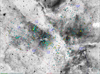 |
Fig. 1. Negative image of the Great Carina Nebula by Robert Gendler and Stephane Guisard showing the location of the whole census of massive stars in the GES surveyed area presented in this work. Yellow and cyan colors indicate O and B-type stars, respectively. Green, red, purple, and pink colors have been used to represent the sdO, luminous blue variable (LBV), Wolf-Rayet (WR), and red supergiant (RSG) stars, respectively. Small filled-circles refer to the GES sample while rhombuses and squares refer to stars from GOSSS/LiLiMarlin and other works (Smith 2006a; Alexander et al. 2016; Preibisch et al. 2021) not present in GES, respectively. Red circles indicate the observing GES pointings while the blue ones indicate the Villafranca groups: O-002 (Trumpler 14), O-003 (Trumpler 16 W), O-025 (Trumpler 16 E), O-027 (Trumpler 15), O-028 (Collinder 228), O-029 (Collinder 232), and O-030 (Bochum 11). The V-shaped extinction lane that dominates the appearance of the nebula is clearly seen crossing the image from top to bottom. |
One important difference between the set studied here and most of the other GES data sets is the existence of a significant nebulosity in the region. Furthermore, the nebular Balmer and He I emission lines are not only strong but are placed on top of important diagnostic stellar absorption lines. For that reason, we devised a specific strategy to eliminate or at least mitigate their influence when we prepared these observations. Each of the four pointings was divided into two subpointings (for a total of eight) with half of the fibers dedicated to stars and the other half to nebulosity. The two subpointings within a given pointing have identical fiber configurations but the field center is displaced by 10″ between the two of them. This means that each star observed in a given subpointing has a nebular counterpart 10″ away that is observed in the other subpointing. One of authors (JMA) of the present paper wrote an IDL code to manually review each star and nebulosity spectral pair and to use the second one to subtract the nebular contribution from the stellar fiber. This strategy is the best possible one given the limitations of the observational setup, but is not ideal, as in some cases nebular emission can change substantially in scales smaller than 10″. This is one of the advantages of long-slit spectroscopy (such as that obtained by GOSSS) over its fiber-fed alternative, as the former allows a sampling of nebular emission closer to the target and at two different locations with respect to the star. In practical terms, this issue becomes important only for faint stars at Hα, as the nebular contribution for bright stars and other relevant lines is usually small.
We examined all of the spectra in our GES datasets to identify OB massive stars (B2 or earlier for dwarfs, B5 or earlier for giants, and all B subtypes for supergiants) and obtained a sample of 234 objects, 18 of which were observed with FLAMES-UVES and 216 with FLAMES-GIRAFFE. The spectrograms are shown in Figs. A.1 and A.2, in the first case at the original 47 000 spectral resolution and in the second case at the 2500 spectral resolution used for spectral classification.
2.2. GOSSS spectroscopy
The GOSSS project was born a decade and a half ago with the idea of obtaining mid- to low-resolution (R ∼ 2500) blue-violet spectroscopy of any optically accessible Galactic object that had ever been classified as an O star in order to confirm its nature and to provide homogeneous spectral classifications for the whole sample. While doing that, GOSSS managed not only to discover a sizable number of new O-type stars but also to reject quite a number of them as being of B type (and even of later types) and to obtain good-quality spectroscopy of several thousand other early-type stars. In the first three major papers, Sota et al. (2011) or GOSSS I, Sota et al. (2014) or GOSSS II, and Maíz Apellániz et al. (2016) or GOSSS III, GOSSS published spectra for 590 O-type stars and for a few later-type objects. Since that time, GOSSS has collected a large number of new spectra, some of them in the Carina Nebula. Of those, eight new GOSSS spectra for O-type stars will appear in the fourth major installment of the project (GOSSS IV, Maíz Apellániz et al. in preparation) but the spectral classifications are already listed here in Table A.2. In this paper, we also present GOSSS spectra for one Wolf-Rayet and 17 early-B stars in Fig. A.3 as a complement to the GES data.
2.3. Spectral classifications
We obtained spectral classifications using the MGB tool (Maíz Apellániz et al. 2012, 2015), which compares the observed spectra with a standard library of OB stars (in this case the GOSSS library; see GOSSS III+IV). This interactive software allows us to vary the spectral subtype, luminosity class, line broadening, and spectral resolving power of the standard spectrum until we obtain the best match. In addition, it also allows us to combine two standard spectra (with different velocities and flux fractions) to fit SB2 systems. The spectral classification was performed for the three types of spectroscopic data (UVES, GIRAFFE, and GOSSS) at the same spectral resolution as that of the GOSSS library, namely 2500. The spectral classifications are given in Table A.2.
There is one specific issue with GIRAFFE spectra and spectroscopic binaries that needs to be discussed. In general, each grating was observed at a different epoch and this generates a problem for spectroscopic binaries, as different lines of the same ion may be at different velocities. We deal with this issue on a case by case basis but in some cases we are only able to provide a poor-quality spectral classification. See Sect. 3.2 for some examples.
2.4. Spectral types from other sources and cataloguing
In addition to those from GES and GOSSS, in Table A.2 we give spectral types from other further sources. The first is LiLiMaRlin (Library of Libraries of Massive-star High-Resolution Spectra, Maíz Apellániz et al. 2019a), which is collecting multi-epoch high-resolution optical+near-infrared (NIR) spectra of massive stars, with over 60 000 epochs to date. For the case of the Carina Nebula, the library currently has FEROS, UVES, and HARPS spectra. LiLiMaRlin is especially useful for the analysis of SB2 and SB3 systems, where finding the right epoch is usually necessary to separate the different components in velocity. One of the LiLiMaRlin spectral types appeared before in Villafranca I but there are also nine whose spectra will appear in GOSSS IV and another 16 whose spectra will appear in Villafranca III. For the two latter papers, those spectral types are listed here for the first time.
Multi-epoch high-resolution spectroscopy such as that from LiLiMaRlin can be used to separate spectroscopic binaries in velocity. If one wants to spatially separate close visual binaries, then what is needed is the combination of high-spatial resolution with spectroscopy, either from the ground (Maíz Apellániz et al. 2018, 2021a) or from space (Maíz Apellániz & Barbá 2020). For the case of the Carina Nebula, we give in Table A.2 the spatially resolved spectral types for HD 93 129 Aa,Ab, one of the most massive systems in the region, obtained with STIS/HST (Maíz Apellániz et al. 2017).
Another source is the already mentioned GOSC, which is a catalog that compiles information about massive stars (with an emphasis on O stars) from different sources. GOSC has a private and a (increasingly growing) public version, which will be heavily updated after GOSSS IV is published. Here we have used the private version of GOSC to search for additional massive stars in the region of interest and provide spectral types. In particular, we include the results from Smith (2006a), a previous census of the massive stars in the Carina Nebula, from Alexander et al. (2016), a spectroscopic survey of the region, and from Preibisch et al. (2021), a NIR spectroscopy survey to identify obscured OB stars.
Besides the flow of information from GOSC to this paper mentioned in the previous paragraph, there will be a flow of information in the opposite direction, as the spectral types here will be included in GOSC. In addition to GOSC, these spectral types will be used to update the Alma Luminous Star Catalog (ALS, Reed 2003), a compilation of (originally) photometric and spectroscopic information for Galactic OB stars. In Pantaleoni González et al. (2021), the original ALS catalog was cross-matched with Gaia DR2 to eliminate the many misidentifications and duplicates present and to provide astrometric information. In a soon-to-be-submitted third paper, the cross-match will be revised with Gaia DR3 information and the catalog will be expanded with new information, such as the one in this paper.
2.5. Gaia EDR3 data
We searched the Gaia EDR3 archive (Brown et al. 2021) for the astrometric and photometric information of the sample in the paper. Gaia EDR3 parallaxes, ϖ, have a zero point, ZEDR3 (Lindegren et al. 2021), that needs to be applied to yield-corrected parallaxes, ϖc. Furthermore, the internal parallax uncertainties are underestimated and have to be converted into external (or true) uncertainties. Here we follow the procedure outlined in Maíz Apellániz et al. (2021b); Maíz Apellániz (2022) to list the corrected parallaxes with their external uncertainties in Table A.1. We also list there the membership of each star to a foreground or background population according to its parallax (see Appendix A for details).
As the inverse of the parallax is a biased estimator of the distance (Lutz & Kelker 1973), one has to make a proper estimation of the distance involving a prior. The prior depends on the analyzed population itself: notoriously, OB stars do not follow the same spatial distribution in the Milky Way as its older populations. Here we use the thin-disk model and prior of Maíz Apellániz (2001, 2005) updated with the parameters of Maíz Apellániz et al. (2008) to calculate the distances and uncertainties of individual stars. See Pantaleoni González et al. (2021) for a comparison among different distance estimates to OB stars using Gaia parallaxes.
Gaia EDR3 provides photometry in three bands, G3, GBP3, and GRP3, with the two last bands being actually the result of integrating spectrophotometry in the wavelength direction. The analysis of previous Gaia data releases (Maíz Apellániz 2017; Maíz Apellániz & Weiler 2018) revealed that the sensitivity curves of the Gaia instrument change with time, leading to slightly different intrinsic photometric values between data releases (each being an average over different time frames). Furthermore, in some cases, the processing introduces small trends and artifacts in the published magnitudes that require corrections. In a paper that will be submitted soon, a team that includes some of the authors of the present paper have computed such an analysis for G3, leading to a corrected value  . In Table A.1, we list the
  and GBP3 − GRP3 values for our sample.
3. Census
Here we present the new census of massive stars in the central region of the Carina Nebula and discuss some individual stars of interest, especially if they have previously received little or no attention. The census itself is presented in two tables in the Appendix already introduced in the previous section. Table A.1 lists the star identifications and coordinates, Gaia EDR3-corrected photometry and parallaxes, and the group identification (see previous section and Fig. 1). Table A.2 gives the spectral classifications from different sources. Disagreements between spectral classifications are sometimes attributable to the nature of spectroscopic binaries caught in different orbital phases but in other cases they are due to differences in data quality (e.g., wavelength range, S/N, uncorrected artifacts) or classification criteria (e.g., choice of lines for classification, standards used, consideration of line broadening). When in doubt, one should consult the published spectrograms, not the spectral types themselves. This is the reason for publishing long Appendices with figures such as the one here.
3.1. Overall properties
The resulting census of stars presented in this work contains 316 massive stars2. We note that, by definition and as stated before, massive OB stars include all O-types and those B2-types or earlier for dwarfs, B5-types or earlier for giants, and all B subtypes for supergiants (I or II luminosity classes). Red supergiants (RSGs), Wolf-Rayet (WR) stars, and some B subtypes close to the OB-star limit (e.g., B2.5 V) are also included in the census for completeness. We have separated stars with distances compatible with Car OB1 from those in the foreground and background, finding four systems in the foreground (one RSG, two B dwarfs and one sdO) and 18 in the background (two O stars, five B supergiants, and 11 B nonsupergiants). These systems are listed in Table A.3.
Of the 294 stellar systems in our census in Car OB1, 74 are of O type, 214 are of nonsupergiant B type, and 6 are of WR or nonO supergiant (II to Ia) spectral class (these are listed in Table A.4). We note that other WR stars in Car OB1 fall outside the surveyed area (WR 22, WR 23 and WR 27). Compared to the previous census of the massive stars in the Carina Nebula by Smith (2006a), we have significantly increased the content of known OB stars in the region. Considering only the area surveyed in this work, the number of 105 OB stellar systems with spectral types as late as B2 reported by Smith (2006a) has been increased by a factor of 2.8.
There are three RSGs in the field of view: HD 93 420, HD 93 281, and HDE 303 310 (= RT Car), all of them included in the study of Humphreys et al. (1972). These are the second, fifth, and sixth  brightest sources, as the bolometric correction in that photometric band is significantly lower for RSGs than for O-type and WR stars. η Car is in a different luminosity category and is almost two magnitudes brighter in
  than the brightest RSG. HD 93 420 is three sigmas3 closer to us in parallax than 0.44 mas, which is the limit we are using to include a star in Car OB1, and that places it in the foreground (but closer to Car OB1 than to us). The other two stars have parallaxes compatible with being in Car OB1, HD 93 281 in Villafranca O-028 (Collinder 228), and HDE 303 310 in Villafranca O-029 (Trumpler 15). In this paper, we list their new spectral classifications from Villafranca III, derived from recently obtained FEROS spectra. The classification for HD 93 420 is identical to that of Humphreys et al. (1972) but the other two are of slightly later type, with HDE 303 310 at M3 Iab and HD 93 281 at M1.5 Iab. We see no sign of the alleged B-type companion for HD 93 281 (see Humphreys et al. 1972) other than the strong Hα emission.
The three RSGs are not the only sign of the existence of previous generations of massive-star formation in Car OB1 and its immediate foreground. We also find in our sample evolved B stars such as HDE 305 535, HDE 305 452, CPD −58 2605, CPD −59 2469, and CPD −59 2504. We find only one B-supergiant of luminosity class I at the distance of Car OB1 in the footprint of this paper, namely HDE 305 530 (the two stars by Damiani et al. (2017) classified as B I, namely 2MASS J10440384−5934344 and 2MASS J10452875−5930037, are classified here as B2V and B1.5Vp, respectively), but a number of B and later-type supergiants are observed in its vicinity (Villafranca III). All of this establishes the existence not only of those older massive stars but also of the supernova explosions associated to those star-formation episodes. It has been known for a long time that the gas in the foreground of some of the OB stars in Carina shows the most complex kinematics in any Galactic sightline (Walborn & Hesser 1975; Walborn 1982a; Walborn et al. 2002), with up to 26 individual components and a range of velocities between −388 km s−1 and +127 km s−1. Those components must have been produced by supernova explosions whose progenitors were evolved massive stars. The remaining three RSGs and the evolved B stars must be just a small part of the previous massive populations. Those complex kinematics are the main reason why the interstellar lines present in the spectra of the Carina OB stars are so strong (Penadés Ordaz et al. 2011, 2013), as the spread in velocity yields a more advantageous curve of growth. Because of the additional Routly-Spitzer effect (Routly & Spitzer 1951, 1952), the Ca II H+K lines are especially strong for these stars, making them deviate strongly from the relationship between extinction and the equivalent width (EW) derived from other sightlines.
3.2. Individual stars
The Carina Nebula field has a large number of interesting stars – starting with η Car – that have been analyzed in the past (see, e.g., Damineli et al. 2000, 2008; Iping et al. 2005). Our goal in this subsection is not to discuss such objects, but to present new interesting objects that have received little or no attention in the past or new aspects of old objects that are mentioned for the first time.
QZ Car Aa,Ac. This complex system (Sánchez-Bermúdez et al. 2017; Rainot et al. 2020) is the brightest of O-type in the Carina Nebula. Mayer et al. (2001) identified this object as an SB1E+SB1 system and measured the two periods as 5.991 d (eclipsing) and 20.735 96 d (noneclipsing). In GOSSS II, the system was classified as O9.7 Ibn with no resolved components4. In GOSSS IV, the system is determined to be O9.7 Ib + O9 II: using LiLiMaRlin, but the authors note that the secondary luminosity class is poorly determined, possibly as the result of contamination by one of the additional stars. The high luminosity of the two primaries coupled with the smaller contribution of the secondaries explains why this system is located at the top of the optical–luminosity zone of the O-type stars in the Carina Nebula. The Gaia EDR3 parallax uncertainty is relatively large.
HD 93 129 Aa,Ab. This system was spatially resolved by Maíz Apellániz et al. (2017) using HST/STIS and determined to be composed of two O2 If* stars, with one of them having a companion in a tight orbit, likely a late-O star. The orbit is highly eccentric and passed through periastron in  (del Palacio et al. 2020). Given that the periastron took place at a 3D separation of just 18.6 ± 1.0 AU (when the system was first spatially resolved in 1996 it was ∼375 AU), an order of magnitude (or even less) smaller than the expected semi-major axis of the inner orbit, and the high eccentricity, it is possible that the system has transitioned from an elliptic orbit to a hyperbolic trajectory and a possible ejection from Villafranca O-002 (Trumpler 14). If that had happened, this could be another example of an orphan cluster where the most (in this case, two) massive stars of a cluster are ejected through a dynamical interaction (Maíz Apellániz et al. 2022b). Further observations are needed, especially with HST/STIS later in this decade (if it is still operational) when Aa and Ab are expected to reach plane-of-the-sky separations of ∼40 mas.
HD 93 403. Rauw et al. (2000) classified this SB2 system as O5.5 I + O7 V. In GOSSS II, the two components could not be resolved and it received a classification of O5.5 III(fc) var. In GOSSS IV, it is now kinematically resolved and classified as O5 Ifc + O7.5 V using either GOSSS or LiLiMaRlin data, that is, the primary is slightly earlier and the secondary slightly later compared to Rauw et al. (2000). The Gaia EDR3 parallax uncertainty is relatively large.
HDE 305 520. Alexander et al. (2016) classified this system as B1 Ia. In Villafranca III, we use LiLiMaRlin data to reclassify it as B0.7 Iab. This Villafranca O-028 object is the only B supergiant at the distance of Car OB1 in our sample.
V572 Car. Rauw et al. (2001) classified this SB3 system in Villafranca O-025 (Trumpler 16 E) as composed of an O7 V + O9.5 V inner eclipsing binary and an outer B0.2 IV star. In GOSSS III, only two components were seen and received an O7.5 V(n) + B0 V(n) classification. With the new data, we now detect the system as an SB3: O6.5 Vz + B0 V + B0.2 V in LiLiMaRlin data in GOSSS IV and O6.5 Vz + B0 V + B0.5: V in UVES. As is the case for HD 93 403, the primary is slightly earlier and the secondary slightly later compared to the original classification. The outer star has been detected in NIR long-baseline interferometry and is currently further monitored (see Gosset et al. 2014).
CPD −59 2554. This system was classified as O9.5 IV in GOSSS II. Using LiLiMaRlin in GOSSS IV and UVES here it is now found to be an SB2. In both cases, the spectral classification is O9.2 V + B1: V.
HD 93 342. This object was considered as a Villafranca O-027 (Trumpler 15) member by Smith (2006a), where it received a classification as O9 III. Alexander et al. (2016), on the other hand, classified it as B1 Ia, and in Villafranca III we reclassify it as B1.5 Ib using LiLiMaRlin data, confirming it is a B-type supergiant and not an O star. Its Gaia EDR3 distance is  kpc, placing it beyond Car OB1, something that is consistent with its red color (it is the brightest OB star in our sample with GBP3 − GRP3 > 1.0).
HD 93 056. Alexander et al. (2016) classified this system as O9 V + B2 V. In Villafranca III, we use LiLiMaRlin data to reclassify it as B1: V:n. Furthermore, in the UVES data, no He II is detected (either 4542, 4686, or 5412), as expected for an SB2 system composed of a late-O and an early-B star, even if caught at a disfavorable phase.
HD 93 501. Alexander et al. (2016) classified this system as B0 V. In Villafranca III, we use LiLiMaRlin data to reclassify it as B1.5: III:(n)e. Its Gaia EDR3 distance is  kpc, placing it in the foreground.
CPD −59 2592. Alexander et al. (2016) classified this object as B1 Ib. In Villafranca III, we use LiLiMaRlin data to reclassify it as B2.5 Ia. Its Gaia EDR3 distance is  kpc, placing it beyond Car OB1, something that is consistent with its red color (it is the brightest OB star in our sample with GBP3 − GRP3 > 1.2).
HDE 305 439 A,B. With GIRAFFE data, we classify the A component as B0 Ia. Its Gaia EDR3 distance is  kpc, placing it beyond Car OB1, something that is consistent with its moderately red color (it is the fourth brightest OB star in our sample with GBP3 − GRP3 > 0.7). In Villafranca III, we use LiLiMaRlin data to classify the B component located 3
 7 away as B0.7 Ib. Its parallax is consistent with being at the same distance, making the system a likely pair of B supergiants.
HDE 305 535. This object was classified as B2.5 V by Alexander et al. (2016). Here we derive a classification of B4 III(n) from UVES data, which leads to an absolute magnitude that is more consistent with its spectral type and low extinction.
HD 93 343. Rauw et al. (2009) classified this SB2 system as O7-8.5 + O8. In GOSSS III, the two components could not be resolved and it received a classification of O8 V. In GOSSS IV, it is now kinematically resolved and classified as O7.5 Vz + O7.5: V(n).
CPD −59 2636 A,B. This system is a visual binary with a 0 3 separation and Δm = 0.6 mag in which both components are spectroscopic binaries (Albacete Colombo et al. 2002): A (A+B in Albacete Colombo et al. 2002) is an SB2 with a 3.6284 d period and B (C in Albacete Colombo et al. 2002) is an SB1 with a 5.034 d period. Those authors gave a spectral classification of O7 V + O8 V to A and of O9 V to B. In GOSSS II, the authors were only able to give two spectral types as O8 V + O8 V but with GES we are able to see the three components in an UVES single epoch and derive spectral types of O7.5 V + O8 V + O8 V. Further epochs are needed to solve the small discrepancies with the Albacete Colombo et al. (2002) classification. Gaia EDR3 does not provide a parallax for CPD −59 2636 A,B, which is common for a visual binary of this separation and magnitude difference, but it is likely a member of Villafranca O-025 (Trumpler 16 E).
HDE 305 534. Alexander et al. (2016) identified this system as a spectroscopic binary and classified it as B0 V + B0 V. In Villafranca III, we use LiLiMaRlin data to confirm it is an SB2 and reclassify it as B0 V + B1: V.
HDE 305 543. Gagné et al. (2011) identified this system as a spectroscopic binary and classified it as B0 V + B0 V. In Villafranca III, we use LiLiMaRlin data to confirm it is an SB2 and reclassify it as B0.2 V(n) + B1: V(n).
HDE 303 312. We detect this object as a SB2 for the first time with GIRAFFE and assign it spectral types O9.5 III + B0.5: V. In GOSSS II, where it was likely caught at a disfavorable phase, it had received the intermediate type O9.7 IV. It was already known to be an eclipsing binary with a 9.4109 d period (Otero 2006).
CPD −58 2649 A. We classify this system as an SB2 with spectral types O9.7 III: +B0: V in GOSSS IV with GOSSS data. With GIRAFFE data, we can only give a poorer classification of O9.5: + B0: due to the different phases in each grating; in any case both components are clearly later than the O7 V + O8 V of Alexander et al. (2016). There is a visual companion detected in Gaia EDR3 with a separation of 1 2 that, though relatively weak, may contaminate the GOSSS and GES spectra.
ALS 15 860. This object was considered as a Villafranca O-027 (Trumpler 15) member by Smith (2006a), where it received a classification as O9 I-II. Using either the GOSSS or GES data here we classify it as B1 Iab. Its Gaia EDR3 distance is  kpc, placing it beyond Car OB1, consistent with its red color (it is the brightest OB star in our sample with GBP3 − GRP3 > 1.8).
CPD −58 2634. We classify this object as B1.5 V using GIRAFFE data. Its Gaia EDR3 distance is  kpc, placing it in the foreground. Its parallax is consistent with being at the same distance as HD 93 501.
CPD −59 2591. This system in Villafranca O-028 (Collinder 228) was classified as an SB2 with spectral types O8 Vz + B0.5: V both in GOSSS III using GOSSS spectroscopy and in GOSSS IV using LiLiMaRlin data. Here it is seen as SB2 but the classification is of poorer quality because of the multiple epochs of the GIRAFFE data.
CPD −59 2535. This system was classified as B2 V by Alexander et al. (2016) but there is no GES, GOSSS, or LiLiMaRlin data. Its Gaia EDR3 distance is  kpc, placing it in the background.
2MASS J10424476−6005020. A GIRAFFE spectrum is used to identify this system as an SB2 with the spectral types B0.2 V + B0.2 V. In a GOSSS spectrum no double lines are seen, likely because of an unfavorable epoch, and the resulting spectral classification is a poorer B0: IV. Its Gaia EDR3 distance is  kpc, placing it in the background. Its red color is consistent with the measured distance.
2MASS J10460477−5949217. This object in Villafranca O-030 (Bochum 11) is classified as an O star for the first time with GIRAFFE data. It has a moderately high extinction and a spectral classification of O9.7 V(n). The spectrum could be a composite of a late-O and an early-B stars but more epochs are needed to test that hypothesis.
2MASS J10444803−5954297. This object is an Oe star with strong Balmer emission and no previous classification as O type. As usual with Oe stars, spectral classification is of poor quality and we can only give O7: Ve using GIRAFFE and O8: Ve in GOSSS IV using GOSSS. The Gaia EDR3 parallax indicates a background object at a distance of  kpc.
kpc.
CPD −59 2618. Alexander et al. (2016) classified this system as B2 V. A GIRAFFE spectrum indicates it is of an earlier subtype and with an anomalous composition, yielding a classification of B1: V(n)p He rich. In Villafranca III, we use LiLiMaRlin data to confirm the helium enrichment and to further discover it is an SB2, classifying it as B0.7: V(n)p He rich + B1: V.
ALS 15 225. We identify this star in Villafranca O-028 (Collinder 228) as a He-rich B star for the first time using both GIRAFFE and GOSSS spectroscopy here.
V662 Car. Niemelä et al. (2006) identified this system as an O5.5 Vz + O9.5 V SB2 and an eclipsing binary with a period of 1.41355 d. In GOSSS III, it was classified as O5 V(n)z + B0: V. The GIRAFFE data shows there are two separate components in He II and both narrow, with a third component clearly separated in He I, making it an SB3. However, given the multiple epochs in the GIRAFFE data, we can only classify it as O+O+B. Both O stars have narrow lines, and so the GOSSS III (n) suffix is likely due to a combination of two O stars. The second O star is likely a third light not participating in the orbit and appears to be of mid-O subtype. The first O star has He II 4542 > He II 4471 and should be close to O5. Thorough characterization of this system requires further high-resolution spectroscopy covering the whole classification range in a single epoch at large velocity separation.
ALS 15 203 A,B. In Villafranca II, this Villafranca O-002 (Trumpler 14) object was identified as an SB3 with a classification of B0 V + B + B. In GIRAFFE, we see some double lines but He II lines are very weak, invalidating the Vijapurkar & Drilling (1993) classification as O7 V. As Gaia EDR3 detects two sources of similar magnitude separated by 1 2 (confirmed by HST imaging), we reanalyzed the GOSSS long slit with the best seeing and proper orientation and were able to spatially separate the two visual components. ALS 15 203 A is an SB2 with a spectral classification of B0.5 V + B1: V, which corresponds to those of the secondary and tertiary in Villafranca II, and ALS 15 203 B has a classification of B0 V, which corresponds to the primary in Villafranca II. There is a hint of emission at the bottom of Hβ for ALS 15 203 B but it is unclear whether this is of stellar origin or is due to an incorrect nebular subtraction. In any case, this SB3 system is now a SB2+Cas following the SBS nomenclature of Maíz Apellániz et al. (2019b)
2MASS J10435902−5933196. We identify this star in Villafranca O-002 (Trumpler 14) as a He-rich B star for the first time using GIRAFFE data.
2MASS J10441829−5942296. We identify this star in Villafranca O-003 (Trumpler 16 W) as a He-rich B star for the first time using GIRAFFE data.
2MASS J10453807−5944095. This object in Villafranca O-025 (Trumpler 16 E) is identified as an O star for the first time here using GIRAFFE data. It has an O8 Vz spectral classification and a high extinction.
2MASS J10440744−5916399. This is a background object caught as an SB2 but with an uncertain GIRAFFE classification of O9.7: + B0.5:. If confirmed, it would be another new O star. The derived Gaia EDR3 distance is  kpc.
kpc.
[ESK2003] 148 = [S87b] IRS 41. This system was first identified as an O-type candidate at the distance of Car OB1 by Damiani et al. (2017). The identification was based on a photometric analysis with CHORIZOS (Maíz Apellániz 2004) and resulted in values of Teff = 42.4 ± 4.4 kK, E(4405 − 5495) = 1.351 ± 0.020 mag, and R5495 = 4.92 ± 0.09, which indicates an O star with both large color excess and anomalous extinction. It is classified as O9.2 V(n) both in GOSSS IV and here using GIRAFFE. The Teff therefore appears to be slightly lower than the value measured with CHORIZOS. It is highly reddened but with a position and parallax consistent with being in Villafranca O-025 (Trumpler 16 E), likely slightly behind the rest of the cluster and immersed in the molecular cloud.
2MASS J10471498−5953374. A GIRAFFE spectrum yields the spectral classification B6: IIIe, with a double-peaked emission line in Hα but no emission in Hγ (no other Balmer lines are covered by the GIRAFFE data). The derived Gaia EDR3 distance is  kpc, placing it in the background.
2MASS J10443089−5914461. This object is classified as a highly extinguished supergiant with spectral type O7.5 II(f) using either GOSSS data in GOSSS IV or GIRAFFE data here. Alexander et al. (2016) classified it as O8 V but it is clearly not a dwarf. It has a large parallax uncertainty: it could not be discarded as being in Car OB1, but is more likely a background object.
2MASS J10453185−6000293. This highly extinguished O star in Villafranca O-030 (Bochum 11) is identified as an O star for the first time. It receives a spectral classification of O7.5 V in GOSSS IV using GOSSS data and a slightly later one of O8.5 V here using GIRAFFE data. The latter is rather noisy but some lines show signs of asymmetry, indicating a possible spectroscopic binary.
[ARV2008] 217 = [S87b] IRS 42. This object is one of the most interesting discoveries in this paper. Using GOSSS data in GOSSS IV, the authors give it an O3: III: spectral classification and using GIRAFFE here we arrive at the same classification but with an (n) suffix. In both cases the O3: classification is based on the apparent absence of He I 4471 but the two spectra are too noisy to provide a more accurate classification based on the N lines. Therefore, it is a new member of the limited family of Galactic O stars with spectral types earlier than O4. It was first identified as an O-type candidate at the distance of Car OB1 by Damiani et al. (2017). The CHORIZOS analysis there gives Teff = 42.0 ± 4.2 kK, E(4405 − 5495) = 1.932 ± 0.021 mag, and R5495 = 4.60 ± 0.06, that is, an early-type O star with both large color excess and anomalous extinction. This latter analysis is in good agreement with the spectral classification. The object position and parallax for this object are consistent with it being in Villafranca O-025 (Trumpler 16 E), making it the earliest O-type star there.
2MASS J10431945−5944488. The Gaia EDR3 parallax for this object yields  pc, clearly making it a foreground (and very blue) object. The existence of broad Hγ and He II lines indicates that the spectrum is dominated by an sdO. However, He II 4542 and He II 4686, observed at different epochs, have different velocities and some lines appear to originate in a later-type star. Therefore, the system is a spectroscopic binary.
High-extinction population of Preibisch et al. (2021). These latter authors list several stars that were too faint to be observed with GIRAFFE in the blue-violet region. Regarding their Gaia EDR3 parallaxes, most of them are similar to or smaller than that of Car OB1 but with larger uncertainties. There is only one with negative parallax, which is likely a background object: 2MASS J10452648−5946188 (=[HSB2012] 3994), which was already identified as a highly extincted B star by Damiani et al. (2017) using CHORIZOS.
4. Results and discussion
4.1. The observed CMD and completeness
We first discuss the observed Gaia EDR3 CMD for the sample of 316 objects in this paper, which is plotted in the first panel of Fig. 2. Of those, only four are located in the foreground but two of them are in distinct regions of the CMD: HD 93 420, a RSG in the upper right, and 2MASS J10431945−5944488, a sdO in the lower left. The main group, that is, the 294 objects in Car OB1, does not follow the typical isochrone of a cluster or association because of the strong differential extinction present in the region. The majority concentrate between the extinguished isochrones that correspond to E(4405 − 5495) of 0.3 and 0.6 (assuming an R5495 of 4.5) but some are significantly more extinguished than that, including the four Preibisch et al. (2021) objects outside the frame towards the lower right. The 18 background objects have, on average, a higher extinction than the Car OB1 population, an expected effect of the extinction associated with the Carina Nebula. They appear mixed in the vertical direction with the Car OB1 population but one should consider that if we plotted absolute magnitude on the vertical axis, they would move upwards. For example, five of the 18 objects are B supergiants.
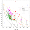 |
Fig. 2. Gaia EDR3 CMD for the stars of our census. First panel (see the following page for the second one): Gaia EDR3 CMD for the stars with spectral types in this paper. Different symbols and colors are used to represent stars with parallaxes compatible with being (or otherwise assumed to be) in the foreground (4), in the background (18), or in Car OB1 (294). Of the Car OB1 stars, 6 are of Wolf-Rayet or nonO supergiant (II to Ia) spectral class, 74 are of O type, and 214 are of nonsupergiant B type. Four of the Preibisch et al. (2021) stars are outside the frame towards the lower right due to their high extinction. Black lines show the average main sequence at a distance of 2.35 kpc with no extinction and with values of E(4405 − 5495) of 0.5, 1.0, 1.5, and 2.0 (labeled) using the extinction law of Maíz Apellániz et al. (2014) with a value of R5495 of 4.5, which is typical of the region but with a large dispersion (Maíz Apellániz & Barbá 2018). Solid orange lines show the R5495 = 4.5 extinction tracks for average MS stars of Teff of 52.5 kK, 30 kK, and 20 kK (labeled), respectively. The dotted orange line shows the R5495 = 3.0 extinction track for Teff = 30 kK. |
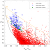 |
Fig. 2. Second panel (see previous page for the first one): Equivalent plot but for all Gaia EDR3 stars in the region of interest with corrected parallaxes that are compatible with the distance to Car OB1 and positive, and with catalog values of GBP3 − GRP3. The plotted objects are classified according to whether they are located inside or outside of the area limited by GBP3 − GRP3 = 1.0 and the R5495 = 4.5 extinction track for average MS stars with Teff = 20 kK. Stars inside that area are further divided into those matched with objects in the first panel (154) and those unmatched (19). We note that an additional three stars inside the above-mentioned area in the first panel (HD 93 129 Ab, CPD −59 2636 A,B, and ALS 19 740) plus η Car outside of that area are not shown either because they are not included in Gaia EDR3 or have no parallaxes there. |
The majority of the stars lie between the R5495 = 4.5 extinction tracks for average MS stars of Teff = 20 kK and 52.5 kK stars. A significant fraction lie below the track of Teff = 20 kK because of a combination of different effects: an average-age B2.5 V star can have a Teff somewhat lower than 20 kK; ZAMS stars should be lower in the CMD than average-age ones; and the extinction tracks for R5495 > 4.5 (which is known to be appropriate for some stars in the Carina Nebula; see Maíz Apellániz & Barbá 2018) are steeper than the plotted ones. Above the extinction track of Teff = 52.5 kK, we find ten Car OB1 stars: η Car, the two RSGs, WR 24, four O supergiants, and HD 93 250 A.B (a close binary with two very early-type components; see Le Bouquin et al. 2017), that is, all of the objects that are expected to be there.
The most striking feature of the first panel of Fig. 2 is how well the Car OB1 O and B stars are separated in the CMD, with the O stars mostly above the average-age extinction track of Teff = 30 kK for R5495 = 4.5 and the B stars below it. This is indirect confirmation of the quality of the spectral classifications. The separation is not perfect but it is not expected to be for several reasons: B giants and supergiants (plus some early B and some early B binaries) are expected to be above the average-age extinction track of Teff = 30 kK for R5495 = 4.5 and late O-dwarfs near the ZAMS below that track. In addition, variations in R5495 among sightlines should produce some mixing, as low values of R5495 can move B stars into the O-star territory and high values of R5495 can move O stars into the B-star territory. Examples of the latter possibility are two of the stars from the Preibisch et al. (2021) sample, 2MASS J10454595−5949075 and 2MASS J10452013−5950104. If they are confirmed to be normal O dwarfs, their value of R5495 should be high.
When building a census, one of the most important questions to be addressed is how complete it is and this is especially important when the sample is built from multiple sources such as in this paper. To answer this question, we plotted in the second panel of Fig. 2 all the Gaia EDR3 sources found within the footprint that have positive corrected parallaxes consistent with being at the distance of Car OB1 and that have catalog values of GBP3 − GRP3. The second panel shows that the first panel shows just a small part of a moderately extinguished well-populated main sequence. In addition to that main sequence, a significant population of red stars is present. By comparison with the first panel, some of those are extinguished OB stars but a comparison with other Galactic sightlines indicates that most of them must be intrinsically red stars. For example, the diagonal series of stars that follows the extinction track of Teff = 30 kK around GBP3 − GRP3 ∼ 1.5 is the red-clump extinction sequence; these are ubiquitously seen in the Galactic plane when plotting absolute magnitude in the vertical axis (as we are effectively doing here by selecting a population consistent with being at the same distance). This latter sequence starts around GBP3 − GRP3 ∼ 1.1 for zero extinction and here we are just seeing it with an extinction distribution that is not significantly different from that of the OB stars in Car OB1.
Given the dominance of the late-type population for red colors (something that needs to be addressed with additional data such as NIR photometry), we do not have the means to determine how complete the sample is for high extinctions. Indeed, this is why a paper as recent as Preibisch et al. (2021) was able to find several new O stars in Car OB1: thick dust clouds can easily hide OB stars if no IR data are available, and even if they are, finding OB stars in such an environment is not always straightforward. Therefore, we concentrate on the low- and moderate-extinction part of the sample, defined as those OB stars with GBP3 − GRP3 < 1.0 (just to the left of the point where the first red clump stars are expected to appear). Since for fainter stars one expects any sample to be less complete, we also restrict the completeness analysis to the region above the extinction track of Teff = 20 kK in Fig. 2. In other words, we are assessing how complete the sample is regarding low- and moderate-extinction O and early-B stars.
We cross-matched the two samples (the one used throughout this paper and the full Gaia EDR3 one) inside that area and found 154 coincidences. Three objects in the main sample are not present in the Gaia EDR3 sample either because they lack parallaxes (CPD −59 2636 A,B and ALS 19 740) or because they are completely absent (HD 93 129 Ab). We note that η Car would also be absent if it were inside that area. Gaia EDR3 is relatively complete barring a few small-separation binaries. As for the other way around, 19 systems in the Gaia EDR3 sample are not present in the main one (green stars in the second panel). Of those, five have large external parallax uncertainties (> 0.1 mas), are therefore unlikely to be real Car OB1 members. Therefore, we estimate that our sample is around 90% complete for low- and moderate-extinction O and early B systems. Furthermore, the location of the 19 green stars in the second panel of Fig. 2 – all of them below the extinction track of Teff = 30 kK – suggests that those missing objects are likely of early-B type. Therefore, we conclude that we are missing very few or even no low or moderate O-type systems in Car OB1 within our footprint in our sample. As mentioned above, this may not be the case for objects with high extinction. In any case, the 74 Car OB1 O-type systems in this paper represent the largest nearly complete sample of objects of that spectral type in any part of a Galactic OB association.
4.2. Binary fraction
It is well known that multiplicity among massive stars is ubiquitous. Commonly, multiplicity is divided into that which is detected through spectroscopy (velocity changes and differences) and that which is revealed by imaging (or visual multiplicity), and it is important to indicate which one is being used, as some previous studies have conflated them and caused confusion. In GOSSS II, we analyzed the population of Galactic southern stars and found that 65%–91% of them are multiple stars of one type or another, with the values for spectroscopic and visual multiples being 50%–60% and 30%–76%, respectively. One consequence of those numbers is that a significant fraction (at least 15%) are at the same time spectroscopic and visual multiples, and most of those involve three stars, as in 2014 the number of pairs detected simultaneously with spectroscopy and imaging was relatively low. An analysis of known multiple O stars in the northern hemisphere (Maíz Apellániz et al. 2019a) confirmed the trend towards systems of three or more stars and revealed that simple binaries are a minority once spectroscopic and visual multiples are included. For example, hierarchical triples composed of a short-period (less than 1 month) system orbited by a companion in a long-period (years or more) orbit are relatively common.
In the census presented here, we find 20 spectroscopic binary systems containing at least one O-type star (listed in Table A.5), one of them located in the background. There are six new systems reported for the first time in this work, either from GES and/or GOSSS IV observations. Excluding the background system, the total number of O stars in the 19 systems of Car OB1 is 30. This represents a fraction of 0.35 (30 out of a total of 85 O-stars; see Table 2 where binary statistics and fractions for the spectroscopic systems containing at least one O-type star in the different Villafranca groups are summarized). This number is still far from those reported in GOSSS II and also from the 0.44 fraction of O-type stars in binaries quoted by Sana & Evans (2011) or even the slightly higher value of 0.50 indicated by Sana (2017). This indicates that there is a significant number of binaries still to be identified in the region. Nevertheless, we highlight that the multiplicity statistics reported in this work are incomplete. We only report double-line spectroscopic binaries. Visual binaries are not considered and only a small fraction of the sample has significant multi-epoch coverage for single-line spectroscopic binary detection. In spite of this, we significantly increase the fractions quoted by Sana & Evans (2011) in Trumpler 14 and Trumpler 16, for which these authors quoted fractions of zero and 0.48, respectively (see Table 2).
Binary statistics and fractions for the spectroscopic systems containing at least one O-type star present in the census.
In addition, we find 18 spectroscopic binary systems formed by early B-type stars, one of them a background system and 13 new binary detections from GES, GOSSS, and LiLiMaRlin observations (see Table A.6). Figure 3 shows an example of the new spectroscopic binary detections from GES spectra at their original resolution. The Si III triplet at λ4552-68-75 Å is shown for binary late-O (a and b panels) and early-B (c and d panels) systems. See figures in Appendix A for full spectra details.
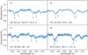 |
Fig. 3. Example of new spectroscopic binary systems reported in this work: Si III line profiles from GES spectra shown at their original resolution. For reference, P and S letters indicate the positions of the primary and secondary components, respectively. See figures in Appendix A for full spectra details. |
4.3. The spectroscopic n-qualifier as an indicator of rotation
As stated in Sect. 2.3, the MGB tool has been used for the spectral classification of GES data. This tool allows the user to obtain not only the spectral subtype and luminosity classification, but also spectral peculiarities and the rotation index. Broadening is denoted by (n), n, nn, and nnn indexes, progressing from slightly broadened to more and even more broadened lines. Therefore, this qualifier has been traditionally interpreted as a sign of high rotational velocity. As a consistency check, we determined the projected rotational velocity of stars with this qualifier in order to know whether or not there is a 1:1 relationship between the two.
To this aim, we used iacob-broad, a user-friendly tool for the line-broadening characterization of OB stars (Simón-Díaz & Herrero 2007, 2014). It is based on a combined Fourier transform (FT) and the goodness-of-fit (GOF) method, which allows us to easily determine the stellar projected rotational velocity (v sin i) and the amount of extra broadening (vmac) from a specific diagnostic line. The FT technique is based on the identification of the first zero in the Fourier transform of a given line profile (Gray 2008; Simón-Díaz & Herrero 2007). The GOF technique is based on a comparison between the observed line profile and a synthetic one that is convolved with different values of v sin i and vmac to obtain the best-fit by means of a χ2 optimization. The main advantage of this methodology is that we obtain two independent measurements of the v sin i (resulting from either the FT or the GOF analysis) whose comparison is used as a consistency check and to better understand problematic cases. As metallic lines do not suffer from strong Stark broadening or nebular contamination, they are best suited for obtaining accurate v sin i values. GIRAFFE setups cover the Si III λ4552 diagnostic line, while UVES/FEROS/HARPS setups cover this latter plus the O III λ5592 diagnostic line. In cases where none of these are present, or they are too weak, we then use the nebular-free or weakly contaminated He I lines (He I λ4387, λ4471, λ4713).
Figure 4 presents the v sin i histogram of the OB stars included in our census with any broadening index in their spectral classification (see Table A.2). Mean v sin i values for (n), n, nn, and nnn are 206, 265, 317, and 392 km s−1, respectively, which confirms the trend that the higher the rotation index the higher the projected rotational velocity. However, we find a significant overlap in the ranges of projected rotational velocity. For example, the (n)- and n-type stars peak at the same bin: between 200 and 250 km s−1; and the fastest n-star rotates 88 km s−1 faster than the slowest nn-star (but the distribution of (n)-stars is slanted towards the left from that point, while that of n-stars is slanted towards the right). There are two likely explanations for the overlap. On the one hand, a non-negligible fraction of these stars could be found to be spectroscopic binaries, as such broadened lines may prevent us from detecting binary line profiles when multi-epoch observations are not available. On the other hand, the sample is dominated by B1-B2.5 dwarfs, which have few intrinsically deep and narrow lines in the analyzed wavelength range (which is only a part of the standard blue-violet classification range), making the n-type indexes more unreliable than for for example O stars or B supergiants.
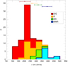 |
Fig. 5. v sin i histogram of those OB stars with any rotation index in their spectral classification. Broadening is denoted by (n), n, nn, and nnn indexes, progressing from slightly broadened to more broadened lines. Points and horizontal lines at the top of the figure indicate the mean v sin i value for each rotating group and the corresponding dispersion, respectively. |
4.4. Runaway candidates
Benefiting from the high-precision astrometry that Gaia EDR3 provides in Carina, we investigated the proper motions of the stars in our census to identify bona fide runaways as a first step for future studies. Following the ideas of de Mink et al. (2013) (who propose that fast-rotating stars are the product of post-interacting binaries and therefore could also have been ejected from binary systems in which the mass donor exploded as a supernova), we are interested in exploring whether or not there is a connection between O and B-type stars with the spectroscopic n-qualifier5 and the runaway status.
The proper motion distribution for each Villafranca group is shown in Fig. 5. We define group centers through an iterative process assuming the average values of each group member, but excluding detected binaries, objects with a renormalized unit weight error (RUWE) > 1.4, and those stars that do not comply with the proper-motion constraint described below. For reference, group proper motions in α* and δ derived in this work and those from the Villafranca II and III are shown in Table 3. As in Villafranca II, we find the proper motion of O-025 to be different from that of O-003, indicating that both groups in Trumpler 16 are well separated. We iteratively filter stars with proper motions larger than the mean values for each group by more than three sigma. To this aim, we calculated  for each group, deriving a final mean σg of 0.342 mas a−1 and thus a three-sigma value of 1.03 mas a−1. We find four stars with the n-qualifier in their spectral classification that do not meet the imposed constraint (those stars falling outside the circles in Fig. 5). Three of them (2MASS J10440866–5933488 in O-002, CPD -59 2541 in O-028 and 2MASS J10451588–5929563 in O-029) can be considered firm runaway candidates. However, we note that the large RUWE value for CPD -58 2657 (in the O-027 group) indicates inaccurate astrometric measurements (see Table A.7). The remaining stars with the n-qualifier are homogeneously distributed around the core motion of each group. Interestingly, the two extreme very fast B rotators of our sample, ALS 15 248 and 2MASS J10433865–5934444, which both rotate at v sin i > 450 km s−1, do not show peculiar proper motions, and so are consistent with the main values of each group. We also find four further runaway candidates that are not included in the group with the n-qualifier but show peculiar proper motions. Two of them are RSG stars. We note that two stars identified in Villafranca I as possible runaway stars ejected from Trumpler 14 (HDE 303 313 and ALS 16 078) spatially fall in the gaps of the redefined Villafranca groups. Therefore, they have been labeled as just Car OB1 members and are not discussed here6.
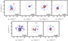 |
Fig. 6. Proper-motion distribution from Gaia EDR3 astrometry for all the stars of our census in each assigned Villafranca group. Orange squares indicate the OB stars analyzed in this work that are rotating at v sin i ≥ 200 km s−1. Blue crosses represent identified binary systems. Circles represent proper motion constraints for each group, whose centers μα * ,g and μδ, g are those shown in Table 3 in the central columns. For comparison, red plus symbols indicate group centers from Villafranca II and III works. We note that stars labeled as Car OB1 members are not included in the panels. |
Group proper motions in α* and δ derived in this work and those from the Villafranca II and III works, all based on Gaia EDR3 astrometry.
We therefore identify 4 out of 90 stars with the n-qualifier as candidate runaway objects and another 4 out of 168 without the n-qualifier, which means fractions of 4.4% and 2.4%, respectively7. This points to a connection between runaways and fast rotators, as pointed out by other works (see f.e. de Mink et al. 2013; Holgado et al. 2022, and references therein), particularly if we consider that the viewing angle may be affecting the projected rotational velocities, resulting in less broadened lines. However, given the limitations of our work, further research on this topic (in particular, a distribution of projected rotational velocities and a more detailed study of the runaway condition) is needed in order to obtain a firm conclusion.
Finally, we note that the distribution of binary systems in the proper motion diagram (crosses in Fig. 5) is homogeneous, which is contrary to what might be expected. A similar pattern was found in the Cygnus OB2 association (Berlanas et al. 2020), implying that these systems may still keep their original velocities.
5. Conclusions
We present a new census of massive stars in the central part of Carina, Car OB1, based on high-quality spectroscopic data provided by GES, GOSSS, LiLiMaRlin, and additional sources from the literature. This catalog contains a total of 316 massive stars. We separated stars with distances compatible with Car OB1 (assigning group membership) from those in the foreground and background, finding 4 systems in the foreground and 18 in the background. Of the 294 stellar systems in Car OB1, 74 are of O type, 214 are of nonsupergiant B type, and 6 are of WR or nonO supergiant (II to Ia) spectral class. We estimate that our sample is around 90% complete for low- and moderate-extinction O and early B systems, missing very few or even no O stars within our footprint. The 74 Car OB1 O-type systems quoted in this paper are the largest nearly complete sample of objects of that spectral type in any part of a Galactic OB association.
Among the stellar census, we identified 20 spectroscopic binary systems that contain at least one O-type star. Six of these are new identifications and one is located in the background. The observed binary fraction of O stars found in the Car OB1 region is 0.35, although this number only refers to double-lined spectroscopic binaries and therefore represents a lower limit. Visual binaries are not considered and only a small fraction of the sample has significant multi-epoch coverage for single-lined spectroscopic binary detection. This number should therefore be considered as a lower limit. In addition, we find another 18 spectroscopic binary systems with a B-star primary, 1 of which is a background system, and 13 are new binary detections from GES, GOSSS, and LiLiMaRlin observations.
We explore the correlation between the spectroscopic rotation index, n, and the actual projected rotational velocities of the stars. We find a good correlation of the average v sin i values with the qualitative classification of each group ((n), n, nn, nnn). However, there is significant overlap in their v sin i ranges. We note that it is possible that a non-negligible fraction of these stars are actually spectroscopic binaries contaminating the fast rotators sample.
Finally, we investigated the proper-motion distribution for the sample of those O and B-type stars with a spectroscopic n-qualifier. Our results indicate a connection between runaways and fast rotators. Furthermore, the distribution of binary systems in the proper motion diagram is homogeneously distributed, implying that these systems may still keep their original velocities.
We note that this number does not distinguish between single and binary or multiple stars, and therefore hereinafter we refer to stellar systems when both types are included in the statistics.
The external parallax uncertainty for such a bright star is much larger than the internal uncertainty (Maíz Apellániz 2022), and so the distance in sigmas would also be larger if we were to use the second one.
Some papers quote spectral types for the four components but these are estimates: to our knowledge both spectroscopic binaries are still SB1 and no resolved (spatially or kinematically) spectral types have been determined.
as a proxy for fast rotation, although we emphasize that, even if there is a good correlation with the average v sin i, not all stars with this qualifier have a high projected rotational velocity, as shown in Sect. 4.3.
A direct comparison between the runaway candidates identified in both works must be done with caution because different methods have been used. We note that in Villafranca works, stars are selected as candidate runaway or walkaway objects when their proper-motion points in the opposite direction to that of the center of the group (within some margins; see Villafranca I-II for further details).
We note that detected spectroscopic binary systems, with or without the n-qualifier, have been excluded from the statistics.
Acknowledgments
This paper is based mainly on data products from spectroscopic observations made with ESO Telescopes at the Paranal Observatory under programme ID 188.B-3002. These data products have been processed by the Cambridge Astronomy Survey Unit (CASU) at the Institute of Astronomy, University of Cambridge, and by the FLAMES/UVES reduction team at INAF/Osservatorio Astrofisico di Arcetri. These data have been obtained from the Gaia-ESO Survey Data Archive, prepared and hosted by the Wide Field Astronomy Unit, Institute for Astronomy, University of Edinburgh, which is funded by the UK Science and Technology Facilities Council. This work was partly supported by the European Union FP7 programme through ERC grant number 320360 and by the Leverhulme Trust through grant RPG-2012-541. We acknowledge the support from INAF and Ministero dell’Istruzione, dell’Università e della Ricerca (MIUR) in the form of the grant ‘Premiale VLT 2012’. The results presented here benefit from discussions held during the Gaia-ESO workshops and conferences supported by the ESF (European Science Foundation) through the GREAT Research Network Programme. Additional spectra were obtained using the http://www.lco.cl/irenee-du-pont-telescope/ at the Observatorio de Las Campanas (LCO) and the https://www.eso.org/public/teles-instr/lasilla/mpg22/ at the Observatorio de La Silla (LSO). This work has made use of data from the European Space Agency (ESA) mission https://www.cosmos.esa.int/gaia, processed by the Gaia Data Processing and Analysis Consortium (https://www.cosmos.esa.int/web/gaia/dpac/consortium). Funding for the DPAC has been provided by national institutions, in particular the institutions participating in the Gaia Multilateral Agreement. This research is partially funded by the Spanish Government Ministerio de Ciencia e Innovación and Agencia Estatal de Investigación (MCIN/AEI/10.130 39/501 100 011 033/FEDER, UE) through grants PGC2018-093 741-B-C21/C22, PGC2018-095 049-B-C21/C22 and PID2021-122 397NB-C21/C22. SRB also acknowledges funding by MCIN under the Juan de la Cierva – Formación grant (contract FJC 2020-045 785-I) and NextGeneration EU/PRTR and MIU (UNI/551/2021) through grant Margarita Salas-ULL. AH also acknowledges support by the Severo Ochoa Program through CEX2019-000920-S. EJA also acknowledges financial support from the State Agency for Research of the Spanish MCIU through the ‘Center of Excellence Severo Ochoa’ award to the Instituto de Astrofísica de Andalucía (SEV-2017-0709). MB is supported through the Lise Meitner grant from the Max Planck Society. We acknowledge support by the Collaborative Research centre SFB 881 (projects A5, A10), Heidelberg University, of the Deutsche Forschungsgemeinschaft (DFG, German Research Foundation). This project has received funding from the European Research Council (ERC) under the European Union’s Horizon 2020 research and innovation programme (Grant agreement No. 949173).
References
- Albacete Colombo, J. F., Morrell, N. I., Rauw, G., et al. 2002, MNRAS, 336, 1099 [NASA ADS] [CrossRef] [Google Scholar]
- Alexander, M. J., Hanes, R. J., Povich, M. S., & McSwain, M. V. 2016, AJ, 152, 190 [Google Scholar]
- Banyard, G., Mahy, L., Sana, H., et al. 2023, A&A, in press [arXiv:2210.07149] [Google Scholar]
- Berlanas, S. R., Herrero, A., Martins, F., et al. 2017, in Highlights on Spanish Astrophysics IX, eds. S. Arribas, A. Alonso-Herrero, F. Figueras, et al., 453 [Google Scholar]
- Berlanas, S. R., Herrero, A., Comerón, F., et al. 2018a, A&A, 612, A50 [NASA ADS] [CrossRef] [EDP Sciences] [Google Scholar]
- Berlanas, S. R., Herrero, A., Comerón, F., et al. 2018b, A&A, 620, A56 [NASA ADS] [CrossRef] [EDP Sciences] [Google Scholar]
- Berlanas, S. R., Herrero, A., Comerón, F., et al. 2020, A&A, 642, A168 [NASA ADS] [CrossRef] [EDP Sciences] [Google Scholar]
- Blomme, R., Daflon, S., Gebran, M., et al. 2022, A&A, 661, A120 [NASA ADS] [CrossRef] [EDP Sciences] [Google Scholar]
- Bragaglia, A., Alfaro, E. J., Flaccomio, E., et al. 2022, A&A, 659, A200 [NASA ADS] [CrossRef] [EDP Sciences] [Google Scholar]
- Brown, A. G. A., Vallenari, A., Prusti, T., et al. 2021, A&A, 649, A1 [NASA ADS] [CrossRef] [EDP Sciences] [Google Scholar]
- Clark, J. S., Negueruela, I., Crowther, P. A., & Goodwin, S. P. 2005, A&A, 434, 949 [NASA ADS] [CrossRef] [EDP Sciences] [Google Scholar]
- Crowther, P. A., Schnurr, O., Hirschi, R., et al. 2010, MNRAS, 408, 731 [Google Scholar]
- Damiani, F., Klutsch, A., Jeffries, R. D., et al. 2017, A&A, 603, A81 [NASA ADS] [CrossRef] [EDP Sciences] [Google Scholar]
- Damineli, A., Kaufer, A., Wolf, B., et al. 2000, ApJ, 528, L101 [CrossRef] [Google Scholar]
- Damineli, A., Hillier, D. J., Corcoran, M. F., et al. 2008, MNRAS, 384, 1649 [NASA ADS] [CrossRef] [Google Scholar]
- De Becker, M., Rauw, G., & Manfroid, J. 2004, A&A, 424, L39 [NASA ADS] [CrossRef] [EDP Sciences] [Google Scholar]
- De Becker, M., Rauw, G., Manfroid, J., & Eenens, P. 2006, A&A, 456, 1121 [NASA ADS] [CrossRef] [EDP Sciences] [Google Scholar]
- de Mink, S. E., Langer, N., Izzard, R. G., Sana, H., & de Koter, A. 2013, ApJ, 764, 166 [Google Scholar]
- de Mink, S. E., Sana, H., Langer, N., Izzard, R. G., & Schneider, F. R. N. 2014, ApJ, 782, 7 [Google Scholar]
- del Palacio, S., García, F., Altamirano, D., et al. 2020, MNRAS, 494, 6043 [NASA ADS] [CrossRef] [Google Scholar]
- Evans, C. J., Taylor, W. D., Hénault-Brunet, V., et al. 2011, A&A, 530, A108 [NASA ADS] [CrossRef] [EDP Sciences] [Google Scholar]
- Figer, D. F. 2005, Astrophys. Space Sci. Lib., 327, 89 [NASA ADS] [CrossRef] [Google Scholar]
- Gagné, M., Fehon, G., Savoy, M. R., et al. 2011, ApJS, 194, 5 [CrossRef] [Google Scholar]
- Gilmore, G., Randich, S., Worley, C. C., et al. 2022, A&A, 666, A120 [NASA ADS] [CrossRef] [EDP Sciences] [Google Scholar]
- Gosset, E., Le Bouquin, J.-B., Absil, O., & Southworth, J. 2014, in Binary Systems, their Evolution and Environments, P3 [Google Scholar]
- Gray, D. F. 2008, The Observation and Analysis of Stellar Photospheres (Cambridge University Press) [Google Scholar]
- Herrero, A. 2016, ASP Conf. Ser., 507, 135 [Google Scholar]
- Holgado, G., Simón-Díaz, S., Herrero, A., & Barbá, R. H. 2022, A&A, 665, A150 [NASA ADS] [CrossRef] [EDP Sciences] [Google Scholar]
- Humphreys, R. M., Strecker, D. W., Ney, E. P., et al. 1972, ApJ, 172, 75 [NASA ADS] [CrossRef] [Google Scholar]
- Iping, R. C., Sonneborn, G., Gull, T. R., Massa, D. L., & Hillier, D. J. 2005, ApJ, 633, L37 [NASA ADS] [CrossRef] [Google Scholar]
- Langer, N. 2012, ARA&A, 50, 107 [CrossRef] [Google Scholar]
- Le Bouquin, J. B., Sana, H., Gosset, E., et al. 2017, A&A, 601, A34 [NASA ADS] [CrossRef] [EDP Sciences] [Google Scholar]
- Levato, H., & Malaroda, S. 1982, PASP, 94, 807 [NASA ADS] [CrossRef] [Google Scholar]
- Lindegren, L., Bastian, U., Biermann, M., et al. 2021, A&A, 649, A4 [EDP Sciences] [Google Scholar]
- Lutz, T. E., & Kelker, D. H. 1973, PASP, 85, 573 [Google Scholar]
- Mahy, L., Nazé, Y., Rauw, G., et al. 2009, A&A, 502, 937 [NASA ADS] [CrossRef] [EDP Sciences] [Google Scholar]
- Mahy, L., Rauw, G., De Becker, M., Eenens, P., & Flores, C. A. 2013, A&A, 550, A27 [NASA ADS] [CrossRef] [EDP Sciences] [Google Scholar]
- Mahy, L., Sana, H., Abdul-Masih, M., et al. 2020, A&A, 634, A118 [NASA ADS] [CrossRef] [EDP Sciences] [Google Scholar]
- Mahy, L., Sana, H., Shenar, T., et al. 2022, A&A, 664, A159 [NASA ADS] [CrossRef] [EDP Sciences] [Google Scholar]
- Maíz Apellániz, J. 2001, AJ, 121, 2737 [Google Scholar]
- Maíz Apellániz, J. 2004, PASP, 116, 859 [Google Scholar]
- Maíz Apellániz, J. 2005, ESA Spec. Publ., 179 [Google Scholar]
- Maíz Apellániz, J. 2017, A&A, 608, L8 [NASA ADS] [CrossRef] [EDP Sciences] [Google Scholar]
- Maíz Apellániz, J. 2022, A&A, 657, A130 [NASA ADS] [CrossRef] [EDP Sciences] [Google Scholar]
- Maíz Apellániz, J., & Barbá, R. H. 2018, A&A, 613, A9 [Google Scholar]
- Maíz Apellániz, J., & Barbá, R. H. 2020, A&A, 636, A28 [NASA ADS] [CrossRef] [EDP Sciences] [Google Scholar]
- Maíz Apellániz, J., & Weiler, M. 2018, A&A, 619, A180 [Google Scholar]
- Maíz Apellániz, J., Walborn, N. R., Galué, H. Á., & Wei, L. H. 2004, ApJS, 151, 103 [CrossRef] [Google Scholar]
- Maíz Apellániz, J., Alfaro, E. J., & Sota, A. 2008, ArXiv eprints [arXiv:0804.2553] [Google Scholar]
- Maíz Apellániz, J., Sota, A., Walborn, N. R., et al. 2011, HSA, 6, 467 [Google Scholar]
- Maíz Apellániz, J., Pellerin, A., Barbá, R. H., et al. 2012, ASP Conf. Ser., 465, 484 [NASA ADS] [Google Scholar]
- Maíz Apellániz, J., Evans, C. J., Barbá, R. H., et al. 2014, A&A, 564, A63 [CrossRef] [EDP Sciences] [Google Scholar]
- Maíz Apellániz, J., Alfaro, E. J., Arias, J. I., et al. 2015, HSA, 8, 603 [Google Scholar]
- Maíz Apellániz, J., Sota, A., Arias, J. I., et al. 2016, ApJS, 224, 4 (GOSSS III) [CrossRef] [Google Scholar]
- Maíz Apellániz, J., Sana, H., Barbá, R. H., Le Bouquin, J.-B., & Gamen, R. C. 2017, MNRAS, 464, 3561 [CrossRef] [Google Scholar]
- Maíz Apellániz, J., Barbá, R. H., Simón-Díaz, S., et al. 2018, A&A, 615, A161 [NASA ADS] [CrossRef] [EDP Sciences] [Google Scholar]
- Maíz Apellániz, J., Trigueros Páez, E., Jiménez Martínez, I., et al. 2019a, HSA, 10, 420 [Google Scholar]
- Maíz Apellániz, J., Trigueros Páez, E., Negueruela, I., et al. 2019b, A&A, 626, A20 (LiLiMaRlin) [NASA ADS] [CrossRef] [EDP Sciences] [Google Scholar]
- Maíz Apellániz, J., Crespo Bellido, P., Barbá, R. H., Fernández Aranda, R., & Sota, A. 2020, A&A, 643, A138 (Villafranca I) [NASA ADS] [CrossRef] [EDP Sciences] [Google Scholar]
- Maíz Apellániz, J., Barbá, R. H., Fariña, C., et al. 2021a, A&A, 646, A11 [NASA ADS] [CrossRef] [EDP Sciences] [Google Scholar]
- Maíz Apellániz, J., Pantaleoni González, M., & Barbá, R. H. 2021b, A&A, 649, A13 [NASA ADS] [CrossRef] [EDP Sciences] [Google Scholar]
- Maíz Apellániz, J., Barbá, R. H., Fernández Aranda, R., et al. 2022a, A&A, 657, A131 (Villafranca II) [NASA ADS] [CrossRef] [EDP Sciences] [Google Scholar]
- Maíz Apellániz, J., Pantaleoni González, M., Barbá, R. H., & Weiler, M. 2022b, A&A, 657, A72 [NASA ADS] [CrossRef] [EDP Sciences] [Google Scholar]
- Mayer, P., Lorenz, R., Drechsel, H., & Abseim, A. 2001, A&A, 366, 558 [NASA ADS] [CrossRef] [EDP Sciences] [Google Scholar]
- Meynet, G., & Maeder, A. 2000, A&A, 361, 101 [NASA ADS] [Google Scholar]
- Mohr-Smith, M., Drew, J. E., Napiwotzki, R., et al. 2017, MNRAS, 465, 1807 [Google Scholar]
- Morel, T., Blazère, A., Semaan, T., et al. 2022, A&A, 665, A108 [NASA ADS] [CrossRef] [EDP Sciences] [Google Scholar]
- Morrell, N. I., García, B., & Levato, H. 1988, PASP, 100, 1431 [CrossRef] [Google Scholar]
- Negueruela, I., Clark, J. S., & Ritchie, B. W. 2010, A&A, 516, A78 [NASA ADS] [CrossRef] [EDP Sciences] [Google Scholar]
- Negueruela, I., Alfaro, E. J., Dorda, R., et al. 2022, A&A, 664, A146 [NASA ADS] [CrossRef] [EDP Sciences] [Google Scholar]
- Niemelä, V. S., Morrell, N. I., Fernández Lajús, E., et al. 2006, MNRAS, 367, 1450 [CrossRef] [Google Scholar]
- Otero, S. A. 2006, OEJV, 45, 1 [NASA ADS] [Google Scholar]
- Pantaleoni González, M., Maíz Apellániz, J., Barbá, R. H., & Reed, B. C. 2021, MNRAS, 504, 2968 [CrossRef] [Google Scholar]
- Penadés Ordaz, M., Maíz Apellániz, J., Sota, A., et al. 2011, HSA, 6, 544 [Google Scholar]
- Penadés Ordaz, M., Maíz Apellániz, J., & Sota, A. 2013, HSA, 7, 600 [Google Scholar]
- Preibisch, T., Flaischlen, S., Göppl, C., Ercolano, B., & Roccatagliata, V. 2021, A&A, 648, A34 [NASA ADS] [CrossRef] [EDP Sciences] [Google Scholar]
- Rainot, A., Reggiani, M., Sana, H., et al. 2020, A&A, 640, A15 [NASA ADS] [CrossRef] [EDP Sciences] [Google Scholar]
- Ramírez-Agudelo, O. H., Simón-Díaz, S., Sana, H., et al. 2013, A&A, 560, A29 [NASA ADS] [CrossRef] [EDP Sciences] [Google Scholar]
- Randich, S., Gilmore, G., Magrini, L., et al. 2022, A&A, 666, A121 [NASA ADS] [CrossRef] [EDP Sciences] [Google Scholar]
- Rauw, G., Sana, H., Gosset, E., et al. 2000, A&A, 360, 1003 [NASA ADS] [Google Scholar]
- Rauw, G., Sana, H., Antokhin, I. I., et al. 2001, MNRAS, 326, 1149 [NASA ADS] [CrossRef] [Google Scholar]
- Rauw, G., Nazé, Y., Fernández Lajús, E., et al. 2009, MNRAS, 398, 1582 [NASA ADS] [CrossRef] [Google Scholar]
- Reed, B. C. 2003, AJ, 125, 2531 [NASA ADS] [CrossRef] [Google Scholar]
- Routly, P. M., & Spitzer, L., Jr. 1951, AJ, 56, 138 [NASA ADS] [CrossRef] [Google Scholar]
- Routly, P. M., & Spitzer, L., Jr. 1952, ApJ, 115, 227 [NASA ADS] [CrossRef] [Google Scholar]
- Sana, H. 2017, IAU Symp., 329, 110 [Google Scholar]
- Sana, H., & Evans, C. J. 2011, IAU Symp., 272, 474 [Google Scholar]
- Sana, H., de Mink, S. E., de Koter, A., et al. 2012, Science, 337, 444 [Google Scholar]
- Sánchez-Bermúdez, J., Alberdi, A., Barbá, R., et al. 2017, ApJ, 845, 57 [NASA ADS] [CrossRef] [Google Scholar]
- Simón-Díaz, S. 2010, A&A, 510, A22 [NASA ADS] [CrossRef] [EDP Sciences] [Google Scholar]
- Simón-Díaz, S., & Herrero, A. 2007, A&A, 468, 1063 [NASA ADS] [CrossRef] [EDP Sciences] [Google Scholar]
- Simón-Díaz, S., & Herrero, A. 2014, A&A, 562, A135 [NASA ADS] [CrossRef] [EDP Sciences] [Google Scholar]
- Smith, N. 2006a, MNRAS, 367, 763 [Google Scholar]
- Smith, N. 2006b, ApJ, 644, 1151 [Google Scholar]
- Sota, A., Maíz Apellániz, J., Walborn, N. R., & Shida, R. Y. 2008, in RMxAC, 33, 56 [NASA ADS] [Google Scholar]
- Sota, A., Maíz Apellániz, J., Walborn, N. R., et al. 2011, ApJS, 193, 24 [Google Scholar]
- Sota, A., Maíz Apellániz, J., Morrell, N. I., et al. 2014, ApJS, 211, 10 [Google Scholar]
- Trigueros Páez, E., Barbá, R. H., Negueruela, I., et al. 2021, A&A, 655, A4 [CrossRef] [Google Scholar]
- Vijapurkar, J., & Drilling, J. S. 1993, ApJS, 89, 293 [NASA ADS] [CrossRef] [Google Scholar]
- Walborn, N. R. 1972, AJ, 77, 312 [NASA ADS] [CrossRef] [Google Scholar]
- Walborn, N. R. 1973, AJ, 78, 1067 [NASA ADS] [CrossRef] [Google Scholar]
- Walborn, N. R. 1982a, ApJS, 48, 145 [NASA ADS] [CrossRef] [Google Scholar]
- Walborn, N. R. 1982b, AJ, 87, 1300 [NASA ADS] [CrossRef] [Google Scholar]
- Walborn, N. R. 1995, RMxAC, 2, 51 [NASA ADS] [Google Scholar]
- Walborn, N. R., & Hesser, J. E. 1975, ApJ, 199, 535 [NASA ADS] [CrossRef] [Google Scholar]
- Walborn, N. R., Danks, A. C., Vieira, G., & Landsman, W. B. 2002, ApJS, 140, 407 [NASA ADS] [CrossRef] [Google Scholar]
Appendix A: Tables and spectrograms
In this Appendix, we present tables with information for the stars in the field of the Carina Nebula analyzed in this paper and figures with the spectrograms that have not appeared in previous papers.
Table A.1 (available only in electronic form at the CDS) lists the basic information for the stars: name, coordinates, identifications,  magnitude, Gaia EDR3 parallax, and group membership. Regarding the latter, the following algorithm is used:
-
All stars are initially labeled as Car OB1.
-
A search is done to see if the star is located inside the region of the sky defined by the center and radius of one of the groups defined in Villafranca II or III (Villafranca O-002 = Trumpler 14, Villafranca O-003 = Trumpler 16 W, Villafranca O-025 = Trumpler 16 E, Villafranca O-027 = Trumpler 15, Villafranca O-028 = Collinder 228, Villafranca O-029 = Collinder 232, and Villafranca O-030 = Bochum 11). If found, the membership is changed to that group. We note that, as mentioned in the Villafranca papers, the traditional division into such groups is to some point arbitrary: Villafranca O-002, Villafranca O-025, and Villafranca O-027 are likely real clusters while the rest of the groups are just subassociations of the larger Car OB1. As the apertures in the Villafranca papers are circular, some stars just fall in the gaps and remain labeled as Car OB1.
-
Stars without a parallax or with corrected parallax uncertainties greater than 0.1 mas are given in bold face to indicate that the Gaia EDR3 information is not sufficient to determine their distances. We note that many of those objects are known to be located in Car OB1 for other reasons (e.g., η Car or HD 93 129 Ab).
-
Stars whose parallax is larger than 0.44 mas by more than three sigma are labeled as foreground.
-
Stars whose parallax is smaller than 0.41 mas by more than three sigma or is negative are labeled as background. The limits here and in the previous steps are determined from Villafranca II and III.
Table A.2 (available only in electronic form at the CDS) lists the spectral types for the stars in this paper. Three types of spectral types are given: those derived from Gaia-ESO spectra (all new), those derived from GOSSS spectra (most from previous papers and from GOSSS IV but some new, marked as TW), and those derived from LiLiMaRlin and STIS spectra as well as from the literature (all previously published).
Tables A.3 and A.4 list those stars of the census identified in the foreground or in the background, and those of WR or nonO supergiant (II to Ia) spectral class, respectively. Tables A.5 and A.6 list spectroscopic binary systems identified in our census containing at least one O-type and those formed by early B-type stars, respectively. Table A.7 lists runaway candidates identified in this work.
Stars of the census whose distance is not compatible with Car OB1 and are located in the foreground and in the background. See Table A.2 for reference acronyms.
Stars identified in the Car OB1 region as of WR or non-O supergiant (II to Ia) spectral class. See Table A.2 for reference acronyms.
Spectroscopic binary systems identified in the census containing at least one O-type star. See Table A.2 for reference acronyms.
Spectroscopic binary systems identified in the census formed by early B-type stars. See Table A.2 for reference acronyms.
Proper motions from Gaia EDR3 for the identified runaway candidates.
Figure A.1 shows the UVES spectra, Fig. A.2 the GIRAFFE spectra, and Fig. A.3 the GOSSS spectra.
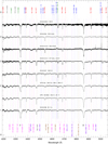 |
Fig. A.1. UVES spectra shown at their original resolution. |
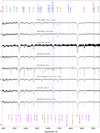 |
Fig. A.1. continued. |
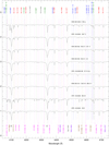 |
Fig. A.2. GIRAFFE spectra shown at a resolution R = 2500. |
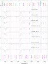 |
Fig. A.2. continued. |
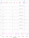 |
Fig. A.2. continued. |
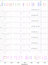 |
Fig. A.2. continued. |
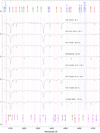 |
Fig. A.2. continued. |
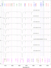 |
Fig. A.2. continued. |
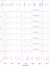 |
Fig. A.2. continued. |
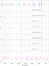 |
Fig. A.2. continued. |
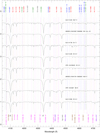 |
Fig. A.2. continued. |
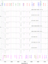 |
Fig. A.2. continued. |
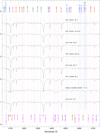 |
Fig. A.2. continued. |
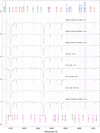 |
Fig. A.2. continued. |
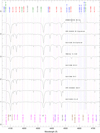 |
Fig. A.2. continued. |
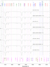 |
Fig. A.2. continued. |
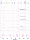 |
Fig. A.2. continued. |
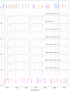 |
Fig. A.2. continued. |
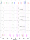 |
Fig. A.2. continued. |
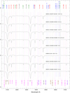 |
Fig. A.2. continued. |
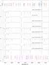 |
Fig. A.2. continued. |
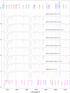 |
Fig. A.2. continued. |
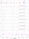 |
Fig. A.2. continued. |
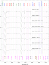 |
Fig. A.2. continued. |
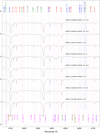 |
Fig. A.2. continued. |
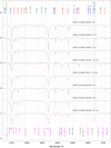 |
Fig. A.2. continued. |
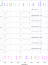 |
Fig. A.2. continued. |
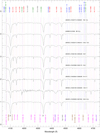 |
Fig. A.2. continued. |
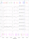 |
Fig. A.2. continued. |
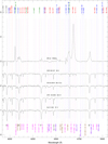 |
Fig. A.3. GOSSS spectra shown at a resolution R = 2500. |
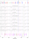 |
Fig. A.3. continued. |
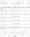 |
Fig. A.3. continued. |
All Tables
Wavelength range and resolving power of the GES spectra obtained with different gratings.
Binary statistics and fractions for the spectroscopic systems containing at least one O-type star present in the census.
Group proper motions in α* and δ derived in this work and those from the Villafranca II and III works, all based on Gaia EDR3 astrometry.
Stars of the census whose distance is not compatible with Car OB1 and are located in the foreground and in the background. See Table A.2 for reference acronyms.
Stars identified in the Car OB1 region as of WR or non-O supergiant (II to Ia) spectral class. See Table A.2 for reference acronyms.
Spectroscopic binary systems identified in the census containing at least one O-type star. See Table A.2 for reference acronyms.
Spectroscopic binary systems identified in the census formed by early B-type stars. See Table A.2 for reference acronyms.
All Figures
|
Fig. 1. Negative image of the Great Carina Nebula by Robert Gendler and Stephane Guisard showing the location of the whole census of massive stars in the GES surveyed area presented in this work. Yellow and cyan colors indicate O and B-type stars, respectively. Green, red, purple, and pink colors have been used to represent the sdO, luminous blue variable (LBV), Wolf-Rayet (WR), and red supergiant (RSG) stars, respectively. Small filled-circles refer to the GES sample while rhombuses and squares refer to stars from GOSSS/LiLiMarlin and other works (Smith 2006a; Alexander et al. 2016; Preibisch et al. 2021) not present in GES, respectively. Red circles indicate the observing GES pointings while the blue ones indicate the Villafranca groups: O-002 (Trumpler 14), O-003 (Trumpler 16 W), O-025 (Trumpler 16 E), O-027 (Trumpler 15), O-028 (Collinder 228), O-029 (Collinder 232), and O-030 (Bochum 11). The V-shaped extinction lane that dominates the appearance of the nebula is clearly seen crossing the image from top to bottom. |
| In the text | |
|
Fig. 2. Gaia EDR3 CMD for the stars of our census. First panel (see the following page for the second one): Gaia EDR3 CMD for the stars with spectral types in this paper. Different symbols and colors are used to represent stars with parallaxes compatible with being (or otherwise assumed to be) in the foreground (4), in the background (18), or in Car OB1 (294). Of the Car OB1 stars, 6 are of Wolf-Rayet or nonO supergiant (II to Ia) spectral class, 74 are of O type, and 214 are of nonsupergiant B type. Four of the Preibisch et al. (2021) stars are outside the frame towards the lower right due to their high extinction. Black lines show the average main sequence at a distance of 2.35 kpc with no extinction and with values of E(4405 − 5495) of 0.5, 1.0, 1.5, and 2.0 (labeled) using the extinction law of Maíz Apellániz et al. (2014) with a value of R5495 of 4.5, which is typical of the region but with a large dispersion (Maíz Apellániz & Barbá 2018). Solid orange lines show the R5495 = 4.5 extinction tracks for average MS stars of Teff of 52.5 kK, 30 kK, and 20 kK (labeled), respectively. The dotted orange line shows the R5495 = 3.0 extinction track for Teff = 30 kK. |
| In the text | |
|
Fig. 2. Second panel (see previous page for the first one): Equivalent plot but for all Gaia EDR3 stars in the region of interest with corrected parallaxes that are compatible with the distance to Car OB1 and positive, and with catalog values of GBP3 − GRP3. The plotted objects are classified according to whether they are located inside or outside of the area limited by GBP3 − GRP3 = 1.0 and the R5495 = 4.5 extinction track for average MS stars with Teff = 20 kK. Stars inside that area are further divided into those matched with objects in the first panel (154) and those unmatched (19). We note that an additional three stars inside the above-mentioned area in the first panel (HD 93 129 Ab, CPD −59 2636 A,B, and ALS 19 740) plus η Car outside of that area are not shown either because they are not included in Gaia EDR3 or have no parallaxes there. |
| In the text | |
|
Fig. 3. Example of new spectroscopic binary systems reported in this work: Si III line profiles from GES spectra shown at their original resolution. For reference, P and S letters indicate the positions of the primary and secondary components, respectively. See figures in Appendix A for full spectra details. |
| In the text | |
|
Fig. 5. v sin i histogram of those OB stars with any rotation index in their spectral classification. Broadening is denoted by (n), n, nn, and nnn indexes, progressing from slightly broadened to more broadened lines. Points and horizontal lines at the top of the figure indicate the mean v sin i value for each rotating group and the corresponding dispersion, respectively. |
| In the text | |
|
Fig. 6. Proper-motion distribution from Gaia EDR3 astrometry for all the stars of our census in each assigned Villafranca group. Orange squares indicate the OB stars analyzed in this work that are rotating at v sin i ≥ 200 km s−1. Blue crosses represent identified binary systems. Circles represent proper motion constraints for each group, whose centers μα * ,g and μδ, g are those shown in Table 3 in the central columns. For comparison, red plus symbols indicate group centers from Villafranca II and III works. We note that stars labeled as Car OB1 members are not included in the panels. |
| In the text | |
|
Fig. A.1. UVES spectra shown at their original resolution. |
| In the text | |
|
Fig. A.1. continued. |
| In the text | |
|
Fig. A.2. GIRAFFE spectra shown at a resolution R = 2500. |
| In the text | |
|
Fig. A.2. continued. |
| In the text | |
|
Fig. A.2. continued. |
| In the text | |
|
Fig. A.2. continued. |
| In the text | |
|
Fig. A.2. continued. |
| In the text | |
|
Fig. A.2. continued. |
| In the text | |
|
Fig. A.2. continued. |
| In the text | |
|
Fig. A.2. continued. |
| In the text | |
|
Fig. A.2. continued. |
| In the text | |
|
Fig. A.2. continued. |
| In the text | |
|
Fig. A.2. continued. |
| In the text | |
|
Fig. A.2. continued. |
| In the text | |
|
Fig. A.2. continued. |
| In the text | |
|
Fig. A.2. continued. |
| In the text | |
|
Fig. A.2. continued. |
| In the text | |
|
Fig. A.2. continued. |
| In the text | |
|
Fig. A.2. continued. |
| In the text | |
|
Fig. A.2. continued. |
| In the text | |
|
Fig. A.2. continued. |
| In the text | |
|
Fig. A.2. continued. |
| In the text | |
|
Fig. A.2. continued. |
| In the text | |
|
Fig. A.2. continued. |
| In the text | |
|
Fig. A.2. continued. |
| In the text | |
|
Fig. A.2. continued. |
| In the text | |
|
Fig. A.2. continued. |
| In the text | |
|
Fig. A.2. continued. |
| In the text | |
|
Fig. A.2. continued. |
| In the text | |
|
Fig. A.3. GOSSS spectra shown at a resolution R = 2500. |
| In the text | |
|
Fig. A.3. continued. |
| In the text | |
|
Fig. A.3. continued. |
| In the text | |
Current usage metrics show cumulative count of Article Views (full-text article views including HTML views, PDF and ePub downloads, according to the available data) and Abstracts Views on Vision4Press platform.
Data correspond to usage on the plateform after 2015. The current usage metrics is available 48-96 hours after online publication and is updated daily on week days.
Initial download of the metrics may take a while.