| Issue |
A&A
Volume 658, February 2022
|
|
|---|---|---|
| Article Number | A139 | |
| Number of page(s) | 13 | |
| Section | Cosmology (including clusters of galaxies) | |
| DOI | https://doi.org/10.1051/0004-6361/202141748 | |
| Published online | 11 February 2022 | |
First look at the topology of reionisation redshifts in models of the epoch of reionisation
Université de Strasbourg, CNRS UMR 7550, Observatoire Astronomique de Strasbourg, Strasbourg, France
e-mail: emilie.thelie@astro.unistra.fr
Received:
8
July
2021
Accepted:
22
November
2021
Context. During the epoch of reionisation (EoR), the first stars and galaxies appeared while creating ionised bubbles that eventually percolated near z ∼ 6. These ionised bubbles and percolation process are closely scrutinised today because observations of neutral hydrogen will be carried on in the next decade with the Square Kilometre Array radio telescope, for instance. In the meantime, EoR studies are performed in semi-analytical and fully numerical cosmological simulations to investigate the topology of the process, for instance.
Aims. We analyse the topology of EoR models by studying regions that are under the radiative influence of ionisation sources. These regions are associated with peak patches of the reionisation redshift field, for which we measure the general properties such as their number, size, shape, and orientation. We aim to gain insights into the geometry of the reionisation process and its relation to the matter distribution, for example. We also assess how these measurements can be used to quantify the effect of physical parameters on the EoR models or the differences between fully numerical simulations and semi-analytical models.
Methods. We used the framework of Morse theory and persistent homology in the context of the EoR, which was investigated via the DisPerSE algorithm on gas density and redshift of reionisation maps. We analysed different EoR scenarios with semi-analytical 21cmFAST and fully numerical EMMA simulations.
Results. We can distinguish between EoR models with different sources using simple analyses of the number, shape, and size distributions of the reionisation redshift patches. For every model (of the semi-analytical and fully numerical simulations), we statistically show that these bubbles are rather prolate and aligned with the underlying gas filaments. Moreover, we briefly highlight that the percolation process of HII bubbles during the EoR can be followed by studying the reionisation redshift fields with different persistence thresholds. Finally, we show that fully numerical EMMA simulations can be made consistent with 21cmFAST models in this topological framework as long as the source distribution is diffuse enough.
Key words: large-scale structure of Universe / dark ages / reionization / first stars / methods: numerical / galaxies: formation / galaxies: high-redshift
© E. Thélie 2022
 Open Access article, published by EDP Sciences, under the terms of the Creative Commons Attribution License (https://creativecommons.org/licenses/by/4.0), which permits unrestricted use, distribution, and reproduction in any medium, provided the original work is properly cited.
1. Introduction
The epoch of reionisation (EoR) marks the transition of a totally neutral to a fully ionised Universe, whose large-scale structures are composed of filaments, voids, and very dense regions. During the EoR, the first sources of radiation appear and release the photons that are required to ionise the cosmic gas. Light escaping from these first stars and galaxies created HII regions (also known as HII bubbles) that eventually percolated at the end of EoR between z = 5.3−6 (Kulkarni et al. 2019).
This epoch is closely studied today to try to understand, for instance, which types of sources drove the EoR, or how and when the HII bubbles overlapped. Analysing the large-scale topology of the EoR is useful to discover the properties of the objects that drove it, such as the nature of the driving sources of the EoR, their spatial distribution, the timing of their appearance, or the spectrum of their radiation (see e.g. Chardin et al. 2017).
Complementary to studies using the power spectrum, for instance (e.g. Mellema et al. 2006; Dixon et al. 2016; Shaw et al. 2020), many works tried to answer these questions with a topological approach of the EoR. For example, Minkowski functionals (and the derived genus or Euler characteristic) are used to analyse the volume, surface aera, and curvature of ionised and neutral regions, giving information about the shape of these regions and the percolation process (as in e.g. Gleser et al. 2006; Lee et al. 2008; Friedrich et al. 2011; Hong et al. 2014; Yoshiura et al. 2017; Chen et al. 2019). Other studies focused on the size distributions of neutral or ionised regions (also called island size distribution, ISD; and bubble size distribution; BSD, respectively), which characterise the size of neutral islands or HII bubbles and their percolation during the EoR. Examples of methods used in these studies are the friends-of-friends algorithm (Iliev et al. 2006; Friedrich et al. 2011; Lin et al. 2016; Giri et al. 2018, 2019), the spherical average method (Zahn et al. 2007; Friedrich et al. 2011; Lin et al. 2016; Giri et al. 2018), the mean free path method (Mesinger & Furlanetto 2007; Lin et al. 2016; Giri et al. 2018, 2019), and the granulometry method (Kakiichi et al. 2017). The Betti numbers, related to 3D structures of a field (isolated objects, tunnels, and cavities), are also used to probe the topology of ionised bubbles and neutral islands during the EoR (Giri & Mellema 2021). The triangle correlation function (TCF) is another tool for extracting topological information, such as the radius and shape of ionised and neutral bubbles (Gorce & Pritchard 2019). It relies on a three-point correlation function based on the inverse Fourier transform of the bispectrum that describes the phase of the signal of interest.
Upcoming observations from radio interferometers such as the New Extension in Nançay Upgrading loFAR1 (NenuFAR; Zarka et al. 2012) and the low-frequency component of the Square Kilometre Array2 (SKA-Low; see e.g. Mellema et al. 2013) will allow us to map the sky with HI regions through the redshifted 21 cm signal that is emitted during the EoR (Mellema et al. 2015). The SKA will produce 2D tomographic images of the 21 cm emission of the EoR at many redshifts. Geometrical studies can therefore focus directly on the 21 cm fields, for example, using the 21 cm power spectrum (see Kim et al. 2013; Choudhury & Paranjape 2018; Seiler et al. 2019; Pagano & Liu 2020) or the 21 cm bispectrum (see Hutter et al. 2020) to extract topological information, such as the size distribution of ionised bubbles.
In this study, we also propose to explore the EoR through its topology, but using the discrete persistent structure extractor, also called DisPerSE3 (Sousbie 2011). This code relies on discrete Morse theory and persistent homology. By computing gradients and critical points of fields, it extracts geometrical properties, including peaks, walls, filaments, and voids for a 3D field. The persistent homology is used in this algorithm only to focus on significant features, and it takes the noise in data sets into account, for instance, by providing a way to suppress the noise by tuning a persistence level. DisPerSE has been written in order to analyse astrophysical structures, in particular, the large-scale density structures of the Universe. Many studies have extracted and analysed the matter filaments with DisPerSE from cosmological simulations (e.g. Singh et al. 2020; Galárraga-Espinosa et al. 2020; Katz et al. 2020; Song et al. 2021), observations (e.g. Malavasi et al. 2020; Tanimura et al. 2020) or both (e.g. Sousbie et al. 2011). Persistent homology has also been used in phenomenological models of the EoR to study the topology of HII regions (Elbers & van de Weygaert 2019).
In this work, we extract the filaments of the matter density field, but also the peak patches of the redshift of reionisation field or zreion (Battaglia et al. 2013; Deparis et al. 2019) from EoR simulations produced by the semi-analytical code 21cmFAST4 (Murray et al. 2020; Mesinger et al. 2011) and the simulation code électromagnétisme et mécanique sur maille adaptative (EMMA; Aubert et al. 2015). The zreion field is a measure of the redshift at which each point in space has been reionised. It therefore contains spatial and temporal information about the propagation of radiation from sources of reionisation in a single field per simulation. Using DisPerSE, we apply the Morse theory framework to the 3D field of our different models. As detailed below, maxima (peaks) in zreion correspond to the seeds, the first sources, of local reionisations. Peak patches around these seeds represent the extent of their time-integrated radiative influence. Even though we did not investigate them in the current work, walls or filaments in zreion define the regions in which percolation occurred. This approach can complement the approaches that are based on the study of HII regions at a single redshift or a sequence of redshifts. The shape of these zreion patches might give us an indication about the way radiation escapes the galaxies. Their size could inform us about the extent of the radiative influence of the different types of sources, for example, in relation to the large absorption trough in the quasar spectra (Becker et al. 2015) or to understanding the observed strong fluctuations of UV radiation (Chardin et al. 2017). In general, a different long-range influence might be expected from faint or locally sub-dominant sources compared to more dominant emitters. Overall, the Morse theory framework as implemented by DisPerSE provides a solid and reproducible mathematical description of the zreion geometry that could be used to characterise and compare models of the EoR. In this initial study, we gain first insights into the extent of the zreion patches, their shapes, and their relative orientation to the underlying gas distribution. We compare different EoR models from 21cmFAST and EMMA.
We first describe in Sect. 2 the method we employed by presenting our simulations, the reionisation redshift field, the DisPerSE algorithm, and the method we used to extract the orientation and shape of the patches. Afterwards, Sect. 3 shows our first topological analyses: the number of reionisation seeds, and the shape and size of the reionisation patches. Sections 4 and 5 highlight the differences between simulations with different parameters, as well as studies of the orientation of radiation with respect to the underlying density. Section 6 presents a comparison of the topology of the EoR in semi-analytical and cosmological simulations. We finally conclude in Sect. 7. The cosmology parameters used throughout are (Ωm, Ωb, ΩΛ, h, σ8, ns) = (0.31, 0.05, 0.69, 0.68, 0.81, 0.97), as given by Planck Collaboration VI (2020).
2. Method
2.1. Simulated data
First, we obtained 3D cosmological simulations from the semi-analytical code 21cmFAST (version 3.0.3; Murray et al. 2020; Mesinger et al. 2011). 21cmFAST evolves initial density and velocity fields based on the first- or second-order perturbation theory of Zel’Dovich (1970), and provides associated predictions such as temperature, ionisation, 21 cm signal, and radiation fields.
In our case, the ionised gas evolved in a 1893 cMpc3 box at a resolution of 1.483 cMpc3 (or boxes of 1283 cMpc3 h−3 with 1283 cells). Different physical models were studied using two parameters of 21cmFAST: the virial temperature Tvir and the ionising efficiency ζ, as defined by Greig & Mesinger (2015). Tvir is the minimum virial temperature for a halo to start the star formation process. It allows controlling the gas accretion, cooling, and retainment of supernova outflows, and it is related to the halo mass through  . The higher the virial temperature, the higher the halo mass. ζ is the ionising efficiency of high-z galaxies. It defines the number of photons that escape from galaxies, and higher values tend to accelerate the reionisation.
The parameters of our different models are shown in Table 1. We separated the models into two sets of simulations: a set in which ζ and Tvir were varied, which we called the same reionisation history (SRH) set, and a set in which ζ alone was varied, which we called the different reonization history (DRH) set. For the SRH simulations set, virial temperatures were set first before we tuned the ionising efficiency in order to obtain the same reionisation history. Then, the higher Tvir, the larger ζ is in order to maintain the same reionisation history because only haloes with the highest mass radiate, meaning that there are also fewer haloes that release photons. The DRH simulation sets were made in order to analyse the effect of different emissivities and thus reionisation histories. We ran each model 101 times using different seeds in 21cmFAST. The ionisation histories of Fig. 1 are averaged over all the runs of each model. Figure 1 shows the ionised volume fraction of all models.
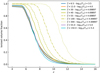 |
Fig. 1. Ionized volume fraction of sets of 21cmFAST simulations with different models, each averaged on their 101 runs. |
Parameters of the 21cmFAST simulated models.
2.2. Reionisation redshift maps
As mentioned in the Introduction, the geometry of ionisation is usually investigated via the ionised fraction distribution xHII(r, z) at a given redshift z or with a sequence of redshifts, where r stands for the 3D position. Here, we rather focus on the reionisation redshift field zreion. It is obtained by saving the redshift at which the gas is considered to be ionised for each position, that is, when the ionisation fraction exceeds a given threshold, which was set at 50%5, as follows:

It incorporates spatial and temporal information about the propagation of radiation during the EoR in a single field (Battaglia et al. 2013; Deparis et al. 2019; Trac et al. 2021) and can be seen as a reciprocal of or dual to the xHII field.
Figure 2 shows an example of a reionisation redshift map extracted from a 21cmFAST simulation. The bluest regions correspond to the places at which the gas was first reionised and can be interpreted as the local seeds of the local reionisation process. Ionization fronts propagated around these zreion peaks towards the reddest regions that reionised later on, forming connected regions of varying shapes and extent: these regions represent the local radiative influence of these local seeds, integrated over time.
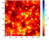 |
Fig. 2. 2D slice at depth z = 64 of the reionisation redshift field extracted from the 21cmFAST simulation (model ζ = 30 and Tvir = 5 × 10⁴ K). |
2.3. DisPerSE
DisPerSE relies on Morse theory in order to analyse the topology of manifolds through the study of differential functions. This code searches for critical points in a field, such as maxima, minima, and saddle points. DisPerSE also looks for the integral lines (or field lines) of the field: they are the tangent curves to the gradient in every point, and always have critical points as origin and destination. As these lines cover the entire space, we can produce a tessellation of the space, creating regions called ascending or descending manifolds. Finally, the set of all ascending or descending manifolds (also known as peak or void patches) is called the Morse complex of a field.
Within DisPerSE, we can tune the so-called “persistence” to control the significance of the topological features found in fields (see Sousbie 2011). This can be considered a significance threshold that separates two critical points, and the local critical points of the field that are not significant enough are ignored. This allows controlling the smoothness of the resulting topological features and can be used to remove the noise in the input data. Figure 3 illustrates the impact of applying a persistence threshold on a 1D field (left column) on which a persistence threshold is applied (right column). We consider a pair of critical points: a minimum (in blue) and a maximum (in red). The distance between the value of the field at these points (green arrows) is compared to the value of the chosen persistence threshold (distance between the two purple dashed lines): if it is higher than the persistence, these extrema are considered when points are detected and assigned to patches. When it is lower, however, they are discarded, as if they were filtered out from the field. In this case, the field becomes topologically smoother.
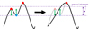 |
Fig. 3. Illustration of the persistence parameter of the DisPerSE algorithm. It shows a 1D function, with red dots as maxima and blue dots as minima. The left column is the actual function to which the persistence threshold is applied, and the right column shows the result after this threshold is applied. The length between the dashed purple lines represents the persistence threshold in that case. The green arrows represent the smoothing of the curve when the corresponding critical points are removed. This illustration is inspired by Sousbie (2011). |
Before we used DisPerSE, the gas density δ(r) and the reionisation redshift zreion(r) were first converted into dimensionless 3D fields by applying the following transformation:

where  and
and  are the mean of each field, and σδ and σzreion are their standard deviation. These transformations allowed us to express the persistence parameter in terms of the deviation of a field to its mean value. They show at how many σ the fields are smoothed from a topological point of view. Moreover, the fields were also filtered with a Gaussian kernel (with a standard deviation of one cell for each field) in order to avoid large patches of constant field values that prevent DisPerSE from running properly.
We first applied the DisPerSE algorithm with a persistence level of 0.5-σ (Sousbie et al. 2011; Codis et al. 2018; Galárraga-Espinosa et al. 2020; Cohn 2021) on the 3D reionisation redshift field of our simulations in order to determine the zreion patches associated with the zreion maxima6. They correspond to the regions that are topologically associated with a given zreion maximum. These regions gather all the cells of the simulations that have a positive gradient towards their maximum. These maxima are the first places to reionise: they are the seeds of local reionisations. Again, these patches are different from the ionised bubbles that are usually mentioned in the literature (see e.g. Chen et al. 2019; Gorce & Pritchard 2019; Giri et al. 2019; Giri & Mellema 2021), which are regions in which hydrogen gas is ionised at a given time. The cells within the patches discussed here are connected through time via the topology of zreion, providing another insight into the propagation of ionisation fronts and into the extent of the influence of the reionisation seeds. Figure 4 shows reionisation redshift maps superimposed on the contours of their segmentation obtained with DisPerSE. The patches are naturally centred around the maxima, are not necessarily spherical, and have different sizes and shapes (we recall that 3D effects can be hidden in these 2D maps) depending on the local specificities of the production and absorption of radiation.
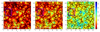 |
Fig. 4. 2D slices of zreion fields extracted from a 21cmFAST simulation. The reionisation redshifts are superimposed on the contours (in black) of the patches from the segmentation obtained with DisPerSE (with a persistence level of 0.5-σ). The three panels represent three models (of the DRH simulations set) with different ζ values: models 3 (ζ = 30), 3−2 (ζ = 55), and 3−4 (ζ = 300), from left to right. |
We are also interested in the filaments of the gas density structures in our models. With DisPerSE, they are detected as the set of points or cells in the density field belonging to arcs that originate in saddle points and end in extrema. We applied this selection to the gas density fields in our simulations using a 0.5-σ persistence level. Figure 5 is an example of a density map from a 21cmFAST simulation superimposed on the filaments detected with DisPerSE. The map is obtained from an average of several slices for better visualisation. The filaments clearly follow the distribution of the gas in the box.
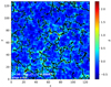 |
Fig. 5. 2D slice of the density field extracted from a 21cmFAST simulation (model ζ = 30 and Tvir = 5 × 10⁴ K). The density is superimposed on the filaments (in black) obtained with DisPerSE (with a persistence level of 0.5-σ). This map is made from an average of many slices to better visualise the filaments. |
2.4. Inertial tensor: A tool for determining the orientation of an object
Our study assesses the shape and size of the reionisation patches, as well as their orientation with respect to the gas filaments. We used inertial tensors, as defined by Tormen (1997),
Here, k scans all of the cells within the patches, i, j ∈ {1, 2, 3} refer to the Cartesian components of the cell position x, and ω is a weight. xref is a point of reference: in our case, it is the geometrical centre of each patch. The eigenvectors of the tensor provide the 3D directions of the extension of the patches, and the eingenvalues provide the typical extent of the cells along these directions. The eigenvector with the highest eigenvalue therefore represents the main axis of a given patch. The same procedure can be applied to the cells belonging to a given gas filament, in order to extract its main orientation.
For zreion patches, we used ωk = 1 because we are only interested in the geometrical shape. The main axis of these patches represents the direction favoured by radiation after it is emitted by the local seed. Presumably, this axis corresponds to the path of least resistance for radiation or is indicative of the geometry of light production as ionisation fronts propagated. Because we are interested in their orientation relative to the reionisation patch they are located in, we set ωk to the cell density for gas filaments and restricted ourselves to cells that are within this reionisation patch.
3. First topological insights
3.1. Number of reionisation patches
Figure 6 shows the number of reionisation patches in every model (accumulating all runs). The parameters that evolve from one simulation to the next, Tvir and ζ, only affect the radiation processes, whereas the density maps are not modified between the different (Tvir, ζ) models, and the filaments are necessarily the same, for instance. The number of reionisation patches (or reionisation seeds) decreases with increasing Tvir (and then ζ; see the top panel of Fig. 6, which shows the SRH set): with higher Tvir, there are fewer emitting haloes because this temperature favours massive haloes (which also produce more photons to maintain a reionisation with the same history). For the DRH simulations set (i.e. with the same emitting haloes, but different ionising efficiencies), the number of reionisation patches as a function of the ionising efficiency parameter presents two regimes. We would have expected the number of reionisation patches to only decrease with increasing ζ: when the sources emit more radiation, the first regions expand rapidly, preventing the smaller and later-formed haloes from creating their own patches. The latter sources are then ionised by external emitters and belong to the patches of these earlier external reionisers. For instance, this behaviour can be seen in the purple boxed patch in the middle and right panels of Fig. 4. It shows reionisation redshift fields for ζ values of 55 and 300 superimposed on their DisPerSE segmentations. As ζ increases, four small patches merge as bright early emitters expand their influence more efficiently and late emitters are externally reionised. However, the number of patches increases as ζ increases from 30 to 55. We verified that this behaviour is an artefact of the way the DisPerSE segmentations are produced in this study. The zreion field was smoothed before being processed by DisPerSE, filtering out small patches of low emitters with weak gradients. As ζ increases, the extent and the gradients are enhanced within these patches, and the gradients are not suppressed by the Gaussian smoothing and the persistence filter. This effect is illustrated in the left and middle panels of Fig. 4. Only two patches are detected within the purple box at low ζ, while four patches can be seen as this parameter is increased to moderately higher values.
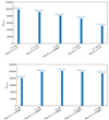 |
Fig. 6. Number of patches detected with DisPerSE (with a persistence level of 0.5-σ) for every model listed in Table 1. Top panel: models of the SRH set, and bottom panel: models of the DRH set. For each model, the patch numbers of every run are added. |
The number of patches is related to the first Betti number β0 of an ionisation field as it represents the number of sources of ionisation (Giri & Mellema 2021). Giri & Mellema (2021) computed the β0 number of their xHII ionisation field throughout the reionisation process for models that varied only the ionising efficiency (see their FN1 and FN2 models and the top left panel of their Fig. 6, where they accumulated the number of sources as xHII grew). These models can be compared to our DRH set models for which we have histories of reionisation (for the lowest ζ models) similar to theirs. They concluded that the β0 numbers of these two models are approximately the same, but with slightly fewer sources, for the model with the highest ζ. We conclude that reionisation patches appear sooner (see Fig. 1), and their total number throughout the reionisation history is lower for the highest ζ models (see Fig. 6), which is consistent with the results of Giri & Mellema (2021).
3.2. Shapes of the reionisation patches
With the eigenvalues given by the inertial tensors, we can compute a number that quantifies the geometrical shape of the patches. Tormen (1997) called it the triaxiality parameter and defined it as follows:

The λi (with i ∈ {1, 2, 3}) are the eigenvalues of the inertial tensors with λ1 ≤ λ2 ≤ λ3. When  , the object is oblate: it has two large dimensions and one small dimension, like a flattened sphere. When
  , the object is triaxial. When
  , the object is prolate: it has one large dimension and two small dimensions, like a rugby ball. The top panel of Fig. 7 shows the probability distribution functions of the triaxiality parameters computed for the reionisation patches of each run of every model. They all return a similar distribution, with a majority of prolate and a minority of oblate patches. The normalisation of these distributions with the fiducial model (bottom panel) reveals small differences between the SRH models, however: with increasing Tvir and ζ, the prolate patches dwindle.
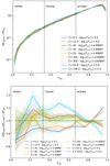 |
Fig. 7. Probability distribution functions of the triaxiality parameter of the reionisation patches of every model (top panel). Bottom panel: same PDFs, but each one of them is divided by one particular model (with ζ = 30 and log10(Tvir) = 4.69897). All the patches of each run for one specific model are accumulated in the two panels. |
These prolate or cigar shapes of the reionisation patches are reminiscent of the “ionised fibre” stage, as it was called in Chen et al. (2019). Using Minkowski functionals, these authors were able to separate the process of reionisation into five stages: an “ionised bubble” stage during which the first isolated ionised bubbles appear, an “ionised fibre” stage during which bubbles start to connect to each other and form a large fibre structure, a “sponge” stage with intertwined ionised and neutral regions, and “neutral fibre” and “neutral island” stages, which are the neutral counterparts of the two first stages. In our segmentations, patches seem to have kept a memory of the fibre shape of the second stage of Chen et al. (2019).
3.3. Size distribution of the reionisation patches
We computed the probability distribution function of the volume of the reionisation patches. Figure 8 shows the PDFs for the two simulation sets. Patches with intermediate volumes dominate the simulation box. The largest volume is limited by the finite size of the box, and the smallest volumes are limted by the resolution. When we compare the different models of the SRH set, the highest virial temperatures favour the ionisation by the more massive haloes that are stronger emitters: it leads to larger but fewer reionisation patches. A similar trend is measured for the DRH set, when ζ becomes large, with fewer and more prominent patches. From our size distributions, a typical radius of patches of ∼10 cMpc h−1 can be extracted, which is consistent for instance with the radii found by Gorce & Pritchard (2019) with their triangle correlation function.
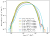 |
Fig. 8. Probability distribution functions of the volume of segmentation patches for each physical model listed in Table 1. Here, all the patches of each run for one specific model are accumulated. |
The size distribution of the patches returns general information about the maximum radius that can be reached by HII regions before percolation during the whole reionisation process. It thus provides insights into the required size for cosmological simulations of the EoR to use the framework described in this work. For example, our PDFs of the patch volumes indicate that our boxes (128 cMpc h−1) do not limit typical-sized patches (10 cMpc h−1), but it is not clear yet what kind of cut-off is applied to these PDFs in the regime of large reionisation patches. It is for instance known that many features in the 21 cm signal only converge at larger scales (200 cMpc h−1 at least; Iliev et al. 2014), and further investigations will be conducted in the future to show how this translates into our reionisation patches.
4. Orientation of the reionisation patches with respect to the gas filaments
This section examines the orientation of the reionisation patches with respect to matter. The directions of the main axis of the gas filaments and the patches they are located in are compared using the eigenvectors of their inertial tensors, computed as explained in Sect. 2.4. To do this, the cosine of the angle between these directions was computed as follows:

Ψzreion, 3 and Ψδ, 3 are the eigenvectors corresponding to the highest eigenvalue of the zreion patches and the filaments, respectively.
4.1. Emitting haloes with different mass ranges and ionising efficiency (SRH set)
We first consider the probability distribution functions of the patch-filament alignment for every model of the SRH set. The PDFs are shown in Fig. 9. For each model, we accumulated the cosines of all of their patches in order to improve the statistics of the result. The top panel shows that most reionisation patches are rather aligned with their gas filament. In addition, there does not seem to be any great difference between the different models of this set. The bottom panel, showing PDFs normalised to the ζ = 30 and Tvir = 5 × 10⁴ K fiducial model, shows the slight variations between the five models. The models are well ordered in the cos(⟨zreion, δ⟩) ∼ 1 regime: in simulations with the smaller emitting haloes, more patches are aligned with the density. Conversely, models with strong emitters more frequently show perpendicular configurations between matter and radiation, but they are still dominated by aligned situations. The grey curve in the top panel corresponds to the model with ζ = 30 and Tvir = 5 × 10⁴ K, for which each filament was rotated with a randomly chosen angle for safety checks. In this case, filaments are oriented randomly, which means that their orientation compared to the radiation is also random. The PDF of this test is rather flat and shows the expected random behaviour.
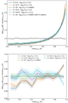 |
Fig. 9. Probability distribution functions of the cosine of the angle between the reionisation patches and their corresponding filaments (top panel). Bottom panel: same PDFs are shown, but divided by the one of the model with ζ = 30 and log10(Tvir) = 4.69897. Each model in which ζ and Tvir varied at the same time is represented here, and all patches of their 101 runs are accumulated in both panels. Top panel: the model with ζ = 30 and log10(Tvir) = 4.69897 is also represented (in grey) with a rotation of filaments for a comparison with total randomness. |
We now know that most reionisation patches are aligned with their filament. In Sect. 2.4, we showed that most reionisation patches have a prolate shape. The question now is whether these behaviours are correlated. Figure 10 is a 2D distribution of the triaxiality parameter versus the cosine of angles between the radiations and filaments for the fiducial model (ζ = 30 and log10(Tvir) = 4.69897). The shape and the orientation of zreion patches are indeed correlated: they are generally prolate and aligned with the filaments. This distribution is very similar for every other model (not shown here). Our simulations therefore show a clear regime of prolate-aligned reionisation patches (see the top right region with  and cos(⟨zreion, δ⟩) ≥ 0.5 of the T versus cos(⟨zreion, δ⟩) space, which includes 46.6% of the total number of patches). Other types of patches are visible as well, even if there are rarer. For example, the opposite of the prolate-aligned patches are the oblate-perpendicular patches to the filaments (see the bottom left region with
  and cos(⟨zreion, δ⟩) ≤ 0.5 of the T versus cos(⟨zreion, δ⟩) space): there are only a few of them (2.36%), and they are in fact patches with butterfly shapes. Figure 11 shows these two types of patches: the pink cells belong to the filament, and the rainbow-coloured cells belong to the reionisation patches. The top panel shows an example of a prolate-aligned region. It clearly shows its prolate shape, and the reionisation patch follows the direction of the filament well. In the bottom panel, the patch looks like a butterfly with two wings that surround the filament: it is easier for the radiation to escape perpendicularly to the filament, as these directions are less dense. Another interesting feature of this butterfly patch is that regions close to the filaments have clearly been reionised earlier, while the reionisation redshift decreases as the distance to the filaments increases. The same behaviour is observed in the prolate-aligned region of the top panel, but in a less impressive manner. These examples clearly show that the sources are located within the filaments or very close to them. This leads to an inside-out scenario of the EoR.
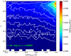 |
Fig. 10. 2D histogram representing the logarithm of the ratio of the number of patches to the total number of patches of the simulation in bins of triaxiality parameter and cosine of the angle between reionisation patches and filaments for the fiducial model (with ζ = 30 and log10(Tvir) = 4.69897). The white full lines are the isocontours of the histogram. The coloured cells of this histogram correspond to non-zero values, and the white cells indicate zero values. |
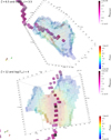 |
Fig. 11. Examples of reionisation patches and their corresponding filament extracted from the segmentations of our simulations: the top panel shows a prolate-aligned region, and the bottom panel shows an oblate-perpendicular or butterfly region. In shades of pink, we show filaments, and rainbow colors indicate the zreion region. The redder the region, the earlier it reionised. In contrast, the bluer the region, the later it reionised. |
The difference between fiber-like and butterfly shapes probably originates in the population of sources within a given patch. Fiber-like regions might include a collection of radiation sources that lie like pearls on a string along the filaments, with similar properties in terms of ignition time, emissivity, and environment: in these situations, the source, located at the reionisation peak of a given patch (i.e. the patch seed) is not different to close-by sources within the same region. The differences in reionisation times values and gradients created by these sources are not sufficient to cause DisPerSE to segment a region into small individual reionisation patches. It rather produces extended patches along filaments. On the other hand, butterfly patches might be the mark of a patch dominated by its seed source (because it is isolated and/or brighter than other local emitters), which alone drives the propagation of ionisation fronts from the very beginning, preferentially along the path of least resistance, perpendicularly to filaments. The latter geometry is clearly sub-dominant in our models, however. This trend can be accentuated by the late reionisation scenario of the SRH dataset (compared to e.g the DRH models): at late times, a greater number of locations are susceptible to host sources, and patches are rarely dominated by a single source. It should be noted that an increase in both Tvir and ζ can boost the propagation of ionisation fronts, cancelling local small variations of reionisation times and gradients around sources along filaments. This would lead to larger coherent patches, and we therefore expect a decrease in the number of fibre-like regions in these cases, as measured indeed in the SRH set.
4.2. Different reionisation histories
We now focus on the simulations of the DRH set (those that vary only ζ for the fiducial Tvir). Changing ζ allows us to study the effect of different histories of reionisation and different halo-ionising efficiencies. Figure 12 shows the PDFs of the cosine of the angle between their reionisation patches and their filaments. At first sight (top panel of this figure), there are no significant differences between the five models: most patches are aligned with their filaments. The PDF ratios of the fiducial model show a weak trend: the higher ζ, the weaker the alignment of the patches with the filaments, and there is a slight increase in the number of perpendicular butterfly patches. This is be consistent with the above hypothesis regarding the origins of the different geometries: DRH models with large ζ (while keeping Tvir constant) attribute strong emissivities to the first and rare sources that seed the patches and let them extend their radiative influence perpendicularly to the filaments at early times.
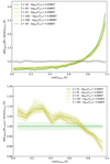 |
Fig. 12. Probability distribution functions of the cosine of the angle between the reionisation patches and their corresponding filaments (top panel). Bottom panel: same PDFs are shown, but they are divided by the one of the model with ζ = 30 and log10(Tvir) = 4.69897. Each of the models that only varied ζ is represented here, and all patches of their 101 runs are accumulated in both panels. The model with ζ = 30 and log10(Tvir) = 4.69897 is also represented (top panel, in grey) with a rotation of filaments for comparison with total randomness. |
5. Effect of the persistence parameter
In the results described above, all the segmentations of the density and the reionisation redshift fields were obtained using DisPerSE with a fixed value of the persistence threshold. In this section, we propose a brief comparison of the main results shown above, but with different persistence values. This comparison is only made for the fiducial 21cmFAST model (ζ = 30 and Tvir = 5 × 10⁴ K) for the sake of brevity, but it is very likely that the conclusions remain the same for every other model.
The segmentations of the density and redshift of reionisation fields (of the fiducial 21cmFAST model) were therefore computed with DisPerSE using four other persistence values, which were 0.625-σ, 0.75-σ, 0.875-σ, and 1-σ. Figure 13 shows the accumulated numbers of reionisation patches found in these fields for every one of the 101 runs. The stronger the persistence, the lower the number of patches, as expected because critical points are more easily merged. This means that in the resulting segmentations with these stronger persistences, the number of critical points is smaller, which explains the smaller number of patches. This behaviour directly affects the volume of the reionisation patches, for which the probability distribution functions are shown in Fig. 14. The correlation of the number of patches and their volume is clearly visible here: the stronger the persistence, the larger the volume of patches and the smaller the number patches because the total volume is conserved.
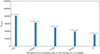 |
Fig. 13. Number of patches in the fiducial model (ζ = 30 and Tvir = 5 × 10⁴ K) that is detected using DisPerSE with different persistence levels. For each one of them, the patch numbers of every run were added. |
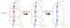 |
Fig. 14. Probability distribution functions of the volume of segmentations patches for the fiducial model (ζ = 30 and Tvir = 5 × 10⁴ K) with the different persistences used in DisPerSE. Here, all the patches of each run for one specific model are accumulated. |
Persistence is related to percolation. For instance, the 1D representation of the persistence in Fig. 3 shows that when a persistence threshold is applied, the leftmost maximum (reionisation seed in our case) disappears and is associated with the other maximum. A weak persistence applied to the reionisation redshift maps allows less prominent and more numerous patches to be taken into account in the final segmentations. Conversely, high persistence values favour the merging of patches by DisPerSE, as shown in Fig. 15. The persistence applied to the reionisation redshift maps can thus be seen as a relative measure of the different timings of creating two patches, and it can therefore follow the percolation process. We could in principle retrieve the relative progression of the fusion of ionised bubbles (regardless of the time), which would provide a complementary view of the time progression of the percolation, which is the subject of many studies in the literature (see e.g. Chen et al. 2019; Giri et al. 2019; Gorce & Pritchard 2019; Giri & Mellema 2021). Elbers & van de Weygaert (2019) pointed out that the persistence can follow the lifetime of a topological feature and then the creation and evolution of structures, which is the percolation process. They showed with simple models that they can follow the stages of reionisation and know in which stage the bubbles are by coupling the persistence homology with the Betti numbers.
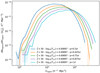 |
Fig. 15. 2D illustration of the percolation process using the persistences. A matter filament is represented in blue with many ionisation seeds (in red) within it. These seeds create their patch of radiative influence (shown in orange), and when the persistence increases (from left to right), smaller patches merge to form larger patches. |
By computing the triaxiality parameter for every new persistence, we can plot the PDFs shown in the top panel of Fig. 16. Generally, all the segmentations with the different persistences behave in the same way: they have a majority of prolate reionisation patches. In the detailed ratios with the 0.5-σ curves (bottom panel of the same figure), however, a trend with increasing persistences is clear: the stronger the persistence, the larger the number of prolate patches. The percolation process therefore favours the merging of patches along filaments and promotes prolate-aligned configurations, with patches like pearls on a string along filaments, as sketched again in Fig. 15. Again, our study of the persistence recalls the process detailed by Chen et al. (2019), who reported that small ionised bubbles grew during their “ionised bubble” stage and merged to form the larger and fibre-like regions during the “ionised fibre” stage. Changing the persistence parameter allows us to retrieve a similar behaviour in our segmentations.
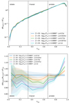 |
Fig. 16. Probability distribution functions of the triaxiality parameter for the fiducial model (ζ = 30 and Tvir = 5 × 10⁴ K) with the different persistences used in DisPerSE (top panel). Bottom panel: same PDFs, but each one of them is divided by one particular model (the fiducial model with a persistence of 0.5-σ). All the patches of each run for one specific model are accumulated in both panels. |
Nevertheless, our segmentations appear to be robust to the changes in persistence, and the main conclusions described in previous sections are unchanged. The shape of the reionisation patches (see Fig. 16) remains very similar, and the orientation of the patches with respect to the filaments is almost unchanged as well, as we show in Fig. 17.
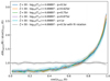 |
Fig. 17. Probability distribution functions of the cosine of the angle between the reionisation patches and their corresponding filaments (as explained in Sect. 2.4) of the fiducial model (ζ = 30 and Tvir = 5 × 10⁴ K) with the different persistences used in DisPerSE, accumulating all patches of every run. The model with the 0.5-σ persistence is also represented (in grey) with a rotation of filaments in order for comparison with total randomness. |
6. Comparison with EMMA simulations
We now compare the topology of EoR simulations obtained with the semi-numerical code 21cmFAST to that of the cosmological simulation code EMMA (Electromagnétisme et Mécanique sur Maille Adaptative, Aubert et al. 2015). EMMA is an adaptive mesh refinement (AMR) code that couples radiative transfer and hydrodynamics. Light is described as a fluid (resolved using the moment-based M1 approximation, Aubert & Teyssier 2008).
The EMMA simulations set we employed was composed of two simulations with a cosmology given by Planck Collaboration VI (2020), without AMR and no reduced speed of light (see Gillet et al. 2021 for more information about the simulations). The difference between the two simulations is the mass resolution of the stellar particles: 107 M⊙ for the one labelled EMMA Mslow and 108 M⊙ for the other simulation. As detailed in Gillet et al. (2021), stellar particles are converted from gas according to a Poissonian process. Cells that convert an amount of gas into stars that is only slightly larger than the stellar mass naturally lead to a stochastic star formation process. Conversely, if the same amount of gas is much larger than the stellar mass particle, it induces a steady stream of particles. As a consequence, the EMMA Mslow model presents a diffuse population of stars, whereas the other model exhibits a stellar biased population focused on the densest cells. For these two simulations, the boxes have 5123 cells for 5123 cMpc3h−3. We then cut these boxes in 64 sub-boxes of 1283 cells and 1283 cMpc3h−3, creating 64 runs of the two EMMA models. The resolution of these sub-boxes was the same as that of the 21cmFAST simulations. Comparisons with the 21cmFAST models were made with 64 runs of each 21cmFAST simulation for consistency.
Figure 18 shows the ionised volume fractions of every simulation of this study. The EMMA simulations are fully ionised approximately at the same time as those of 21cmFAST. With EMMA, however, the reionisation starts later and is more abrupt, which might be explained by the fact that EMMA simulations have larger volumes than the 21cmFAST simulations, with greater voids and larger haloes.
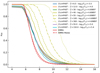 |
Fig. 18. Ionized volume fraction of all the 21cmFAST simulations and the two EMMA simulations having different models, each one of them averaged over 64 runs. |
Again, before we used DisPerSE on the EMMA fields, the same transformations as described in Sect. 2.3 were applied to each sub-box, using the means and the standard deviations of the 5123 cMpc3h−3 boxes instead of those of each sub-grid. We thus took the cosmic variance of the whole box into account. After obtaining the segmentations with DisPerSE with the same persistence as was used for all the 21cmFAST simulations (0.5-σ), the distribution of patch volumes was computed. This is shown in Fig. 19 for every EMMA and 21cmFAST simulation, accumulating 64 runs for each one of them. The EMMA simulations have smaller patches and a greater number of them than the 21cmFAST simulations. The EMMA model with the massive, 108 M⊙, stellar particles is significantly different from the 21cmFAST simulations: the patch size distribution is clearly shifted to smaller volumes with a large number of small patches. The EMMA Mslow model with the less massive, 107 M⊙, stellar particles is more like the 21cmFAST models: the more diffuse source distribution allowed by this setting recovers topological features similar to those of the 21cmFAST models (in which all locations are a potential source of radiation with its own distribution of emitting haloes).
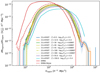 |
Fig. 19. Probability distribution functions of the volume of segmentation patches for every 21cmFAST and EMMA simulation. Here, all the patches of each 64 runs for one specific model are accumulated. |
The tensors and main directions of the reionisation patches and filaments of the EMMA simulations were computed and allowed us to compare the direction of the propagation of radiation with respect to the filament. The top panel of Fig. 20 shows the distributions of the cosine of the angle between these directions for the EMMA and the 21cmFAST simulations. Patches and gas filaments in the EMMA simulation are aligned similarly to the 21cmFAST models, and slightly more aligned in the EMMA Mslow simulation. The bottom panel of Fig. 20 shows the ratio of each PDF of cosines with the fiducial 21cmFAST model. Again, the EMMA Mslow shows very similar PDFs to the 21cmFAST models, which implies that it is possible to recover the same type of behaviour as in semi-analytical simulations with a fully numerical code even if the reionisation occurs differently. Conversely, the EMMA model with massive, 108 M⊙, stellar particles is different in terms of alignments. The scarce, stochastic, and biased distribution of sources in this models leads to many more perpendicular patches than in all the other models. While this model is in reasonable agreement in terms of reionisation history, its topology is quite different: this emphasises that models that present some reasonable global agreement can be vastly different in terms of topology when the details of the source models are not equivalent, for example. The higher star formation stochasticity and the more biased distribution of sources lead to trends that are similar to the higher virial temperatures in the 21cmFAST simulations, with isolated reionisation seeds that dominate their environment more strongly. The shapes of the reionisation patches in the EMMA simulations set are also rather prolate in both simulations, as in the 21cmFAST simulations, and no significant difference between the models was found (not shown here).
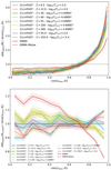 |
Fig. 20. Probability distribution functions of the cosine of the angle between the reionisation patches and their corresponding filaments (top panel). Bottom panel: same PDFs, but divided by the one of the model with ζ = 30 and log10(Tvir) = 4.69897. Each 21cmFAST model is represented here, alongside with the two EMMA simulations, accumulating all patches of 64 runs in both panels. |
7. Conclusions
We have analysed the topological structures extracted from different EoR models made with the 21cmFAST semi-analytical code and the EMMA cosmological simulation code. For this purpose, we used the reionisation redshift and gas density fields. The reionisation redshift field corresponds to the time when the gas has reionised and contains spatial and temporal information about the physical processes during the EoR. To extract the topological information, we used DisPerSE, which applies concepts of Morse theory, to the density field to obtain the filaments of matter and to the reionisation redshift field to segment it into reionisation patches coming from the same seed of local reionisation.
In the 21cmFAST models, the size distributions of the reionisation patches have an average radius of 10 cMpc h−1, quantifying the typical extent of the radiative influence of the seeds of reionisation. In general, an increase in the virial temperature and the ionising efficiency of haloes decreases the number of patches and expands them. This extends the reach of the radiative influence of the seeds of local reionisation.
Using the inertial tensors of the reionisation patches and density filaments, we were able to extract their shape and orientation. We found that the reionisation patches are statistically prolate and aligned with the local gas filaments. Radiation escapes from sources that lie like pearls on a string along the gas filament to reach the zones that reionise last (typically, the voids) in an inside-out manner. A minority of patches shows a butterfly shape. These are oblate patches with radiation that escapes perpendicularly to the local filaments. The difference probably arises from the properties of sources within the patches: if the initial source that defines a reionisation patch is locally dominant in terms of photon output, butterfly shapes can appear, whereas if the initial source is only the first of a collection of rather similar close-by emitters, patches become aligned with the local distribution of matter. We note that the dominant status of a source can depend on many factors (intrinsic emission, escape fraction, density, and configuration of local absorbers) and is therefore likely to be resolution and/or model dependent. Our results, obtained at rather low resolution (1.483 cMpc3), should be revisited, for instance, at higher resolution.
Comparisons of the 21cmFAST segmentations with those obtained from EMMA simulations showed that EMMA simulations can provide results similar to the semi-analytical predictions in terms of patch properties (volume, number) and relative orientations to the filaments of matter. We also find that EMMA simulations with increased bias and stochasticity for star formation can also lead to quite different topologies on the same criteria, even though they present similar reionisation histories.
These results appear to be robust when the persistence parameter with DisPerSE was changed. As the persistence increases and patches are merged, the patches expand and become more prolate. This provides insight into the percolation process of our EoR models directly from a single reionisation map. We find that during the first stages of the reionisation, isolated ionised bubbles appear and merge with time in order to form larger and fibre-like ionised bubbles (Chen et al. 2019). This subject could be further investigated, as it is complementary to standard percolation studies based on sequences of snapshots of ionised fractions maps.
To summarise, the reionisation redshift field contains much spatial and temporal information and is found to be quite useful in the current topological framework. In addition, statistical analyses of this field are quite practical because only one zreion field needs to be extracted from each simulation. We probably only skimmed the potential of the approach developed here. We already described the possibilities offered by the persistence parameter. We could also investigate the halo properties in relation to the host reionisation patches. Moreover, we could work on smaller scales to determine whether the study of the patch geometry (size, shape, orientation) might hold information about the ways in which radiation escapes from galaxies, how far they affect their environment, and even about the time evolution or duty cycles of the photons production (see e.g. Deparis et al. 2019). However, such studies of galaxies or haloes are not possible at the resolution discussed here. Ideally, they would be conducted with models with Cosmic Dawn (CoDa)-like characteristics (Ocvirk et al. 2016). Finally, the zreion field is not a direct observable, and similar analyses might be directly conducted on the topology of 21 cm maps or light cones. These geometrical studies may reveal a way to relate these observations to the timing of the reionisation process.
In practice, DisPerSE computed the ascending 3-manifolds of the field using the integral lines that are related to the maxima of the 3D field (see Sousbie 2011 for more details).
Acknowledgments
We thank Adélie Gorce for her proofreading and her precious questions and advice. We also thank Christophe Pichon for his help with the topological code DisPerSE. Furthermore, we express our gratitude to the referee of this paper for the useful and constructive comments that allowed us to make a more comprehensive and complete paper. This work was granted access to the HPC resources of CINES under the allocations 2020-A0070411049 and 2021-A0090411049 “Simulation des signaux et processus de l’aube cosmique et Réionisation de l’Univers” made by GENCI. This research made use of ASTROPY, a community-developed core Python package for astronomy (Astropy Collaboration 2018); MATPLOTLIB, a Python library for publication quality graphics (Hunter 2007); SCIPY, a Pythonbased ecosystem of open-source software for mathematics, science, and engineering (Virtanen et al. 2020); NUMPY (Harris et al. 2020) and PYTHON (Perez & Granger 2007).
References
- Astropy Collaboration (Price-Whelan, A. M., et al.) 2018, AJ, 156, 123 [Google Scholar]
- Aubert, D., & Teyssier, R. 2008, MNRAS, 387, 295 [NASA ADS] [CrossRef] [Google Scholar]
- Aubert, D., Deparis, N., & Ocvirk, P. 2015, MNRAS, 454, 1012 [Google Scholar]
- Battaglia, N., Trac, H., Cen, R., & Loeb, A. 2013, ApJ, 776, 81 [NASA ADS] [CrossRef] [Google Scholar]
- Becker, G. D., Bolton, J. S., Madau, P., et al. 2015, MNRAS, 447, 3402 [Google Scholar]
- Chardin, J., Puchwein, E., & Haehnelt, M. G. 2017, MNRAS, 465, 3429 [NASA ADS] [CrossRef] [Google Scholar]
- Chen, Z., Xu, Y., Wang, Y., & Chen, X. 2019, ApJ, 885, 23 [NASA ADS] [CrossRef] [Google Scholar]
- Choudhury, T. R., & Paranjape, A. 2018, MNRAS, 481, 3821 [NASA ADS] [CrossRef] [Google Scholar]
- Codis, S., Jindal, A., Chisari, N. E., et al. 2018, MNRAS, 481, 4753 [Google Scholar]
- Cohn, J. D. 2021, ArXiv e-prints [arXiv:2108.02292] [Google Scholar]
- Deparis, N., Aubert, D., Ocvirk, P., Chardin, J., & Lewis, J. 2019, A&A, 622, A142 [NASA ADS] [CrossRef] [EDP Sciences] [Google Scholar]
- Dixon, K. L., Iliev, I. T., Mellema, G., Ahn, K., & Shapiro, P. R. 2016, MNRAS, 456, 3011 [NASA ADS] [CrossRef] [Google Scholar]
- Elbers, W., & van de Weygaert, R. 2019, MNRAS, 486, 1523 [Google Scholar]
- Friedrich, M. M., Mellema, G., Alvarez, M. A., Shapiro, P. R., & Iliev, I. T. 2011, MNRAS, 413, 1353 [NASA ADS] [CrossRef] [Google Scholar]
- Galárraga-Espinosa, D., Aghanim, N., Langer, M., Gouin, C., & Malavasi, N. 2020, A&A, 641, A173 [EDP Sciences] [Google Scholar]
- Gillet, N. J. F., Aubert, D., Mertens, F. G., & Ocvirk, P. 2021, ArXiv e-prints [arXiv:2103.03061] [Google Scholar]
- Giri, S. K., & Mellema, G. 2021, MNRAS, 505, 1863 [NASA ADS] [CrossRef] [Google Scholar]
- Giri, S. K., Mellema, G., Dixon, K. L., & Iliev, I. T. 2018, MNRAS, 473, 2949 [NASA ADS] [CrossRef] [Google Scholar]
- Giri, S. K., Mellema, G., Aldheimer, T., Dixon, K. L., & Iliev, I. T. 2019, MNRAS, 489, 1590 [NASA ADS] [CrossRef] [Google Scholar]
- Gleser, L., Nusser, A., Ciardi, B., & Desjacques, V. 2006, MNRAS, 370, 1329 [NASA ADS] [CrossRef] [Google Scholar]
- Gorce, A., & Pritchard, J. R. 2019, MNRAS, 489, 1321 [NASA ADS] [CrossRef] [Google Scholar]
- Greig, B., & Mesinger, A. 2015, MNRAS, 449, 4246 [NASA ADS] [CrossRef] [Google Scholar]
- Harris, C. R., Millman, K. J., van der Walt, S. J., et al. 2020, Nature, 585, 357 [NASA ADS] [CrossRef] [Google Scholar]
- Hong, S. E., Ahn, K., Park, C., et al. 2014, J. Korean Astron. Soc., 47, 49 [NASA ADS] [CrossRef] [Google Scholar]
- Hunter, J. D. 2007, Comput. Sci. Eng., 9, 90 [NASA ADS] [CrossRef] [Google Scholar]
- Hutter, A., Watkinson, C. A., Seiler, J., et al. 2020, MNRAS, 492, 653 [CrossRef] [Google Scholar]
- Iliev, I. T., Mellema, G., Pen, U. L., et al. 2006, MNRAS, 369, 1625 [NASA ADS] [CrossRef] [Google Scholar]
- Iliev, I. T., Mellema, G., Ahn, K., et al. 2014, MNRAS, 439, 725 [Google Scholar]
- Kakiichi, K., Majumdar, S., Mellema, G., et al. 2017, MNRAS, 471, 1936 [NASA ADS] [CrossRef] [Google Scholar]
- Katz, H., Ramsoy, M., Rosdahl, J., et al. 2020, MNRAS, 494, 2200 [NASA ADS] [CrossRef] [Google Scholar]
- Kim, H.-S., Wyithe, J. S. B., Park, J., & Lacey, C. G. 2013, MNRAS, 433, 2476 [NASA ADS] [CrossRef] [Google Scholar]
- Kulkarni, G., Keating, L. C., Haehnelt, M. G., et al. 2019, MNRAS, 485, L24 [Google Scholar]
- Lee, K.-G., Cen, R., Gott, J. R., III, & Trac, H. 2008, ApJ, 675, 8 [NASA ADS] [CrossRef] [Google Scholar]
- Lin, Y., Oh, S. P., Furlanetto, S. R., & Sutter, P. M. 2016, MNRAS, 461, 3361 [NASA ADS] [CrossRef] [Google Scholar]
- Malavasi, N., Aghanim, N., Douspis, M., Tanimura, H., & Bonjean, V. 2020, A&A, 642, A19 [NASA ADS] [CrossRef] [EDP Sciences] [Google Scholar]
- Mellema, G., Iliev, I. T., Pen, U.-L., & Shapiro, P. R. 2006, MNRAS, 372, 679 [NASA ADS] [CrossRef] [Google Scholar]
- Mellema, G., Koopmans, L. V. E., Abdalla, F. A., et al. 2013, Exp. Astron., 36, 235 [NASA ADS] [CrossRef] [Google Scholar]
- Mellema, G., Koopmans, L., Shukla, H., et al. 2015, Advancing Astrophysics with the Square Kilometre Array (AASKA14), 10 [Google Scholar]
- Mesinger, A., & Furlanetto, S. 2007, ApJ, 669, 663 [Google Scholar]
- Mesinger, A., Furlanetto, S., & Cen, R. 2011, MNRAS, 411, 955 [Google Scholar]
- Murray, S., Greig, B., Mesinger, A., et al. 2020, J. Open Sour. Softw., 5, 2582 [NASA ADS] [CrossRef] [Google Scholar]
- Ocvirk, P., Gillet, N., Shapiro, P. R., et al. 2016, MNRAS, 463, 1462 [Google Scholar]
- Pagano, M., & Liu, A. 2020, MNRAS, 498, 373 [NASA ADS] [CrossRef] [Google Scholar]
- Perez, F., & Granger, B. E. 2007, Comput. Sci. Eng., 9, 21 [Google Scholar]
- Planck Collaboration VI. 2020, A&A, 641, A6 [NASA ADS] [CrossRef] [EDP Sciences] [Google Scholar]
- Seiler, J., Hutter, A., Sinha, M., & Croton, D. 2019, MNRAS, 487, 5739 [CrossRef] [Google Scholar]
- Shaw, A. K., Bharadwaj, S., & Mondal, R. 2020, MNRAS, 498, 1480 [CrossRef] [Google Scholar]
- Singh, A., Mahajan, S., & Bagla, J. S. 2020, MNRAS, 497, 2265 [Google Scholar]
- Song, H., Laigle, C., Hwang, H. S., et al. 2021, MNRAS, 501, 4635 [NASA ADS] [CrossRef] [Google Scholar]
- Sousbie, T. 2011, MNRAS, 414, 350 [NASA ADS] [CrossRef] [Google Scholar]
- Sousbie, T., Pichon, C., & Kawahara, H. 2011, MNRAS, 414, 384 [NASA ADS] [CrossRef] [Google Scholar]
- Tanimura, H., Aghanim, N., Bonjean, V., Malavasi, N., & Douspis, M. 2020, A&A, 637, A41 [NASA ADS] [CrossRef] [EDP Sciences] [Google Scholar]
- Tormen, G. 1997, MNRAS, 290, 411 [NASA ADS] [CrossRef] [Google Scholar]
- Trac, H., Chen, N., Holst, I., Alvarez, M. A., & Cen, R. 2021, ApJ, submitted [arXiv:2109.10375] [Google Scholar]
- Virtanen, P., Gommers, R., Oliphant, T. E., et al. 2020, Nat. Meth., 17, 261 [Google Scholar]
- Yoshiura, S., Shimabukuro, H., Takahashi, K., & Matsubara, T. 2017, MNRAS, 465, 394 [NASA ADS] [CrossRef] [Google Scholar]
- Zahn, O., Lidz, A., McQuinn, M., et al. 2007, ApJ, 654, 12 [NASA ADS] [CrossRef] [Google Scholar]
- Zarka, P., Girard, J. N., Tagger, M., & Denis, L. 2012, in SF2A-2012: Proceedings of the Annual Meeting of the French Society of Astronomy and Astrophysics, eds. S. Boissier, P. de Laverny, N. Nardetto, et al., 687 [Google Scholar]
- Zel’Dovich, Y. B. 1970, A&A, 500, 13 [Google Scholar]
All Tables
All Figures
|
Fig. 1. Ionized volume fraction of sets of 21cmFAST simulations with different models, each averaged on their 101 runs. |
| In the text | |
|
Fig. 2. 2D slice at depth z = 64 of the reionisation redshift field extracted from the 21cmFAST simulation (model ζ = 30 and Tvir = 5 × 10⁴ K). |
| In the text | |
|
Fig. 3. Illustration of the persistence parameter of the DisPerSE algorithm. It shows a 1D function, with red dots as maxima and blue dots as minima. The left column is the actual function to which the persistence threshold is applied, and the right column shows the result after this threshold is applied. The length between the dashed purple lines represents the persistence threshold in that case. The green arrows represent the smoothing of the curve when the corresponding critical points are removed. This illustration is inspired by Sousbie (2011). |
| In the text | |
|
Fig. 4. 2D slices of zreion fields extracted from a 21cmFAST simulation. The reionisation redshifts are superimposed on the contours (in black) of the patches from the segmentation obtained with DisPerSE (with a persistence level of 0.5-σ). The three panels represent three models (of the DRH simulations set) with different ζ values: models 3 (ζ = 30), 3−2 (ζ = 55), and 3−4 (ζ = 300), from left to right. |
| In the text | |
|
Fig. 5. 2D slice of the density field extracted from a 21cmFAST simulation (model ζ = 30 and Tvir = 5 × 10⁴ K). The density is superimposed on the filaments (in black) obtained with DisPerSE (with a persistence level of 0.5-σ). This map is made from an average of many slices to better visualise the filaments. |
| In the text | |
|
Fig. 6. Number of patches detected with DisPerSE (with a persistence level of 0.5-σ) for every model listed in Table 1. Top panel: models of the SRH set, and bottom panel: models of the DRH set. For each model, the patch numbers of every run are added. |
| In the text | |
|
Fig. 7. Probability distribution functions of the triaxiality parameter of the reionisation patches of every model (top panel). Bottom panel: same PDFs, but each one of them is divided by one particular model (with ζ = 30 and log10(Tvir) = 4.69897). All the patches of each run for one specific model are accumulated in the two panels. |
| In the text | |
|
Fig. 8. Probability distribution functions of the volume of segmentation patches for each physical model listed in Table 1. Here, all the patches of each run for one specific model are accumulated. |
| In the text | |
|
Fig. 9. Probability distribution functions of the cosine of the angle between the reionisation patches and their corresponding filaments (top panel). Bottom panel: same PDFs are shown, but divided by the one of the model with ζ = 30 and log10(Tvir) = 4.69897. Each model in which ζ and Tvir varied at the same time is represented here, and all patches of their 101 runs are accumulated in both panels. Top panel: the model with ζ = 30 and log10(Tvir) = 4.69897 is also represented (in grey) with a rotation of filaments for a comparison with total randomness. |
| In the text | |
|
Fig. 10. 2D histogram representing the logarithm of the ratio of the number of patches to the total number of patches of the simulation in bins of triaxiality parameter and cosine of the angle between reionisation patches and filaments for the fiducial model (with ζ = 30 and log10(Tvir) = 4.69897). The white full lines are the isocontours of the histogram. The coloured cells of this histogram correspond to non-zero values, and the white cells indicate zero values. |
| In the text | |
|
Fig. 11. Examples of reionisation patches and their corresponding filament extracted from the segmentations of our simulations: the top panel shows a prolate-aligned region, and the bottom panel shows an oblate-perpendicular or butterfly region. In shades of pink, we show filaments, and rainbow colors indicate the zreion region. The redder the region, the earlier it reionised. In contrast, the bluer the region, the later it reionised. |
| In the text | |
|
Fig. 12. Probability distribution functions of the cosine of the angle between the reionisation patches and their corresponding filaments (top panel). Bottom panel: same PDFs are shown, but they are divided by the one of the model with ζ = 30 and log10(Tvir) = 4.69897. Each of the models that only varied ζ is represented here, and all patches of their 101 runs are accumulated in both panels. The model with ζ = 30 and log10(Tvir) = 4.69897 is also represented (top panel, in grey) with a rotation of filaments for comparison with total randomness. |
| In the text | |
|
Fig. 13. Number of patches in the fiducial model (ζ = 30 and Tvir = 5 × 10⁴ K) that is detected using DisPerSE with different persistence levels. For each one of them, the patch numbers of every run were added. |
| In the text | |
|
Fig. 14. Probability distribution functions of the volume of segmentations patches for the fiducial model (ζ = 30 and Tvir = 5 × 10⁴ K) with the different persistences used in DisPerSE. Here, all the patches of each run for one specific model are accumulated. |
| In the text | |
|
Fig. 15. 2D illustration of the percolation process using the persistences. A matter filament is represented in blue with many ionisation seeds (in red) within it. These seeds create their patch of radiative influence (shown in orange), and when the persistence increases (from left to right), smaller patches merge to form larger patches. |
| In the text | |
|
Fig. 16. Probability distribution functions of the triaxiality parameter for the fiducial model (ζ = 30 and Tvir = 5 × 10⁴ K) with the different persistences used in DisPerSE (top panel). Bottom panel: same PDFs, but each one of them is divided by one particular model (the fiducial model with a persistence of 0.5-σ). All the patches of each run for one specific model are accumulated in both panels. |
| In the text | |
|
Fig. 17. Probability distribution functions of the cosine of the angle between the reionisation patches and their corresponding filaments (as explained in Sect. 2.4) of the fiducial model (ζ = 30 and Tvir = 5 × 10⁴ K) with the different persistences used in DisPerSE, accumulating all patches of every run. The model with the 0.5-σ persistence is also represented (in grey) with a rotation of filaments in order for comparison with total randomness. |
| In the text | |
|
Fig. 18. Ionized volume fraction of all the 21cmFAST simulations and the two EMMA simulations having different models, each one of them averaged over 64 runs. |
| In the text | |
|
Fig. 19. Probability distribution functions of the volume of segmentation patches for every 21cmFAST and EMMA simulation. Here, all the patches of each 64 runs for one specific model are accumulated. |
| In the text | |
|
Fig. 20. Probability distribution functions of the cosine of the angle between the reionisation patches and their corresponding filaments (top panel). Bottom panel: same PDFs, but divided by the one of the model with ζ = 30 and log10(Tvir) = 4.69897. Each 21cmFAST model is represented here, alongside with the two EMMA simulations, accumulating all patches of 64 runs in both panels. |
| In the text | |
Current usage metrics show cumulative count of Article Views (full-text article views including HTML views, PDF and ePub downloads, according to the available data) and Abstracts Views on Vision4Press platform.
Data correspond to usage on the plateform after 2015. The current usage metrics is available 48-96 hours after online publication and is updated daily on week days.
Initial download of the metrics may take a while.