| Issue |
A&A
Volume 648, April 2021
The LOFAR Two Meter Sky Survey
|
|
|---|---|---|
| Article Number | A5 | |
| Number of page(s) | 19 | |
| Section | Extragalactic astronomy | |
| DOI | https://doi.org/10.1051/0004-6361/202039998 | |
| Published online | 07 April 2021 | |
Extremely deep 150 MHz source counts from the LoTSS Deep Fields
1
Leiden Observatory, Leiden University,
PO Box 9513,
2300 RA
Leiden, The Netherlands
e-mail: This email address is being protected from spambots. You need JavaScript enabled to view it.
2
INAF - IRA,
Via P. Gobetti 101,
40129
Bologna,
Italy
e-mail: This email address is being protected from spambots. You need JavaScript enabled to view it.
3
ASTRON, the Netherlands Institute for Radio Astronomy,
Postbus 2,
7990 AA
Dwingeloo, The Netherlands
4
Centre for Astrophysics Research, School of Physics, Astronomy and Mathematics, University of Hertfordshire,
College Lane,
Hatfield
AL10 9AB, UK
5
International Centre for Radio Astronomy Research – Curtin University,
GPO Box U1987,
Perth,
WA
6845, Australia
6
GEPI & USN, Observatoire de Paris, Université PSL, CNRS,
5 Place Jules Janssen,
92190
Meudon, France
7
Department of Physics & Electronics, Rhodes University,
PO Box 94,
Grahamstown,
6140, South Africa
8
Fakultät für Physik, Universität Bielefeld,
Postfach 100131,
33501
Bielefeld, Germany
9
SUPA, Institute for Astronomy, Royal Observatory, Blackford Hill,
Edinburgh,
EH9 3HJ, UK
10
Italian ALMA Regional Centre,
Via Gobetti 101,
40129,
Bologna, Italy
11
INAF-Osservatorio Astronomico di Padova,
Vicolo dell’Osservatorio 5,
35122
Padova,
Italy
12
Astrophysics, Department of Physics,
Keble Road,
Oxford,
OX1 3RH, UK
13
University of the Western Cape,
Private Bag X17,
Bellville,
Cape Town
7535, South Africa
14
Thüringer Landessternwarte,
Sternwarte 5,
07778
Tautenburg, Germany
15
STFC UK Astronomy Technology Centre, Royal Observatory, Blackford Hill,
Edinburgh,
EH9 3HJ, UK
16
Astrophysics & Cosmology Research Unit, School of Mathematics, Statistics & Computer Science, University of KwaZulu-Natal,
Durban
3690, South Africa
Received:
26
November
2020
Accepted:
24
January
2021
Abstract
With the advent of new generation low-frequency telescopes, such as the LOw Frequency ARray (LOFAR), and improved calibration techniques, we have now started to unveil the subgigahertz radio sky with unprecedented depth and sensitivity. The LOFAR Two Meter Sky Survey (LoTSS) is an ongoing project in which the whole northern radio sky will be observed at 150 MHz with a sensitivity better than 100 μJy beam−1 at a resolution of 6′′. Additionally, deeper observations are planned to cover smaller areas with higher sensitivity. The Lockman Hole, the Boötes, and the Elais-N1 regions are among the most well known northern extra-galactic fields and the deepest of the LoTSS Deep Fields so far. We exploited these deep observations to derive the deepest radio source counts at 150 MHz to date. Our counts are in broad agreement with those from the literature and show the well known upturn at ≤1 mJy, mainly associated with the emergence of the star-forming galaxy population. More interestingly, our counts show, for the first time a very pronounced drop around S ~ 2 mJy, which results in a prominent “bump” at sub-mJy flux densities. Such a feature was not observed in previous counts’ determinations (neither at 150 MHz nor at a higher frequency). While sample variance can play a role in explaining the observed discrepancies, we believe this is mostly the result of a careful analysis aimed at deblending confused sources and removing spurious sources and artifacts from the radio catalogs. This “drop and bump” feature cannot be reproduced by any of the existing state-of-the-art evolutionary models, and it appears to be associated with a deficiency of active galactic nuclei (AGN) at an intermediate redshift (1 < z < 2) and an excess of low-redshift (z < 1) galaxies and/or AGN.
Key words: galaxies: evolution / surveys / radio continuum: general
© ESO 2021
1 Introduction
Large-area radio surveys are very important for statistical studies of radio source populations, addressing astrophysical properties and cosmological evolution of radio galaxies, quasars, and starburst galaxies. In the past, several wide-area radio surveys were carried out at low radio frequencies, such as the Cambridge Surveys (3C, 4C, 6C, and 7C at around 160 MHz: Edge et al. 1959; Bennett 1962; Pilkington & Scott 1965; Gower et al. 1967; Baldwin et al. 1985). However, the calibration of low-frequency radio data is challenging due to the direction-dependent, time-varying effects of the ionosphere that affects both the amplitude and the phase of the radio signal. Since these effects are only prominent in the megahertz (MHz) regime, the focus of wide-area and all-sky radio surveys switched to around 1 GHz in the last decades, resulting in the NRAO VLA Sky Survey (NVSS: Condon et al. 1998), the Sydney University Molonglo Sky Survey (SUMSS: Mauch et al. 2003), and the Faint Images of the Radio Sky at Twenty-Centimeters (FIRST) survey (Becker et al. 1995; White et al. 1997).
The higher sensitivity and higher spatial resolution of surveys at gigahertz (GHz) frequencies also allowed us to probe deeper and deeper flux densities, and today we have several deep surveys covering degree-scale fields, which are sensitive to the sub-mJy and μJy radio populations (see e.g., Prandoni et al. 2000a,b, 2006, 2018; Hopkins et al. 2003; Schinnerer et al. 2004, 2007; Hales et al. 2014a; Smolčić et al. 2017). After many years of studies, it is now well established that the sub-mJy radio population has a composite nature. Radio-loud (RL) active galactic nuclei (AGN) are dominant down to 1.4 GHz flux densities of 200–300 μJy, and star-forming galaxies (SFGs) become dominant below about 100–200 μJy (Smolčić et al. 2008; Bonzini et al. 2013; Prandoni et al. 2018; Bonato et al. 2021). A significant fraction of the sources below 100 μJy can also show signatures of AGN activity in the host galaxy at other bands (IR, optical, X-ray), but they rarely display the large-scale radio jets and lobes typical of classical radio galaxies. Most of them are unresolved or barely resolved on a few arcsec scale, that is to say on scales similar to the host galaxy size. The origin of the radio emission in these, so-called radio-quiet, AGN is debated: it may come from star formation in the host galaxy (Padovani et al. 2011, 2015, Bonzini et al. 2013, 2015; Ocran et al. 2017; Bonato et al. 2017) or from low-level nuclear activity (White et al. 2015, 2017; Maini et al. 2016; Herrera Ruiz et al. 2016, 2017; Hartley et al. 2019). Most likely, such AGN are composite systems where star formation and AGN-triggered radio emission coexist over a wide range of relative contributions (e.g., Delvecchio et al. 2017). This scenario is also supported by the modeling work of Mancuso et al. (2017, see also Macfarlane et al., in prep.).
Being sensitive to SFGs up to the epoch of the peak of their activity (z ~ 2−3) and reaching the dominant radio-quiet (RQ) AGN population for the first time, deep radio surveys probing the μJy regime can be used as a very important dust and gas-obscuration-free tool to study both AGN activity and star formation and how they evolve with cosmic time. However, to overcome uncertainties introduced by low statistics, cosmic variance effects (Heywood et al. 2013), and other systematics (Condon et al. 2012), deep-radio surveys that cover wide areas (≫1 deg2) and have multiband ancillary data are needed. Such wide–area surveys are also useful to investigate the role of the environment in driving the growth of galaxies and supermassive black hole (SMBH), and to better trace rare radio source populations.
With the advent of a new generation of low-frequency telescopes and better data processing techniques we can now revisit the radio sky at low-frequency. With the Murchison Widefield Array (MWA; Lonsdale et al. 2009), Wayth et al. (2015) have carried out the GaLactic and Extragalactic All-sky MWA survey (GLEAM; Hurley-Walker et al. 2017), reaching a sensitivity of a few mJy beam−1 at a resolution of a few arcminutes. The GMRT has significantly improved the low-frequency view of the radio sky in terms of sensitivity and angular resolution. This has already been shown in a few low-frequency surveys centered around 150 MHz (e.g., Ishwara-Chandra et al. 2010, Sirothia et al. 2009, Intema et al. 2011, 2017).
The Low Frequency Array (LOFAR; van Haarlem et al. 2013a) is one of the key pathfinders to the Square Kilometre Array (SKA). Most of the LOFAR antennas are based in the Netherlands, with baseline lengths ranging from 100 m to 120 km. Additional remote stations are located throughout various countries in Europe. The longest baseline of LOFAR can provide a resolution of 0.3′′ at 150 MHz. The combination of LOFAR’s large field of view, wide range of baseline lengths, and large fractional bandwidth makes it a powerful instrument for performing large area and deep sky surveys. The LOFAR Two Meter Sky Survey (LoTSS) is an an ongoing project in which the whole northern sky is observed with a sensitivity better than 100 μJy beam−1 at the resolution of 6′′ allowed by the Dutch LOFAR stations. The first data release (DR1) is described by Shimwell et al. (2017, 2019). The LoTSS also includes deeper observations of a number of preselected regions, where the aim is to eventually reach an rms depth of 10 μJy beam−1 at 150 MHz (Röttgering et al. 2011). In order to scientifically exploit these more sensitive surveys (collectively known as LoTSS Deep Fields), complementary multiwavelength data are necessary, most notably to identify the host galaxies of the extra-galactic radio sources and determine their redshift. For this reason observations were focused on fields with the highest quality multiwavelength data available. The Lockman Hole, the Boötes, and the European Large-Area ISO Survey-North 1 (ELAIS-N1) fields are the deepest of the LoTSS Deep Fields so far (see Tasse et al. 2021; Sabater et al. 2021; respectively Papers I and II of this series). All have rich multiwavelength ancillary data, covering a broad range of the electromagnetic spectrum, from X-ray to radio bands.
The Lockman Hole (LH hereafter) is one of the best studied extragalactic regions of the sky. It is characterized by a very low column density of Galactic HI (Lockman et al. 1986) making it an ideal field to study extragalactic sources with deep observations in the mid-IR, FIR, and submillimeter (Lonsdale et al. 2003; Mauduit et al. 2012; Oliver et al. 2012), optical/NIR (Muzzin et al. 2009; Fotopoulou et al. 2012; Hildebrandt et al. 2016), and X-ray (Polletta et al. 2006; Brunner et al. 2008). A variety of radio surveys cover limited areas within the LH region, at several frequencies. The widest deep radio survey so far consists of a 6.6 deg2. 1.4 GHz mosaic obtained with the Westerbork (WSRT) telescope (1σ sensitivity ~10 μJy beam−1; Prandoni et al. 2018). We refer to Prandoni et al. (2018) for a comprehensive summary of the available multifrequency and multiband coverage in this region (see also Kondapally et al. 2021, Paper III of this series).
The Boötes (Boo hereafter) field was originally targeted as part of the NOAO Deep Wide Field Surveys (NDWFS; Jannuzi & Dey 1999) which covers ~9 deg2 in the optical and near infrared (K) bands. Ancillary data is available for this field including X-ray (Murray et al. 2005; Kenter et al. 2005), UV (GALEX; Martin et al. 2003), and mid-infrared (Eisenhardt et al. 2004). Radio observations have also been carried out at 153 MHz with the GMRT (Intema et al. 2011; Williams et al. 2013), at 325 MHz with the VLA (Croft et al. 2008; Coppejans et al. 2015) and at 1.4 GHz with the WSRT (de Vries et al. 2002).
The Elais-N1 (EN1 hereafter) field has deep multiwavelength (0.15–250 μm) data taken as part of many different surveys – optical: the Panoramic Survey Telescope and Rapid Response System; Pan-STARRS (Chambers et al. 2016) and Hyper-Suprime-Cam Subaru Strategic Program (HSC-SSP) survey, u-band: Spitzer Adaptation of the Red-sequence Cluster Survey; SpARCS: Muzzin et al. 2009, UV: Deep Imaging Survey (DIS): Martin et al. 2005, NIR J and K band: the UKIDSS Deep Extragalactic Survey (DXS) DR10 (Lawrence et al. 2007), MIR: IRAC instrument on board the Spitzer Space Telescope: SWIRE; Lonsdale et al. 2003 and The Spitzer Extragalactic Representative Volume Survey (SERVS; Mauduit et al. 2012).
Mahony et al. (2016) presented the first LOFAR 150 MHz map of the LH with a sensitivity of 160 μJy beam−1 at a resolution of 18.7′′ × 16.4′′. Williams et al. (2016) presented the first LOFAR map of the Boo field at a resolution of 5.6′′ × 7.4′′ with an rms of 120 μJy beam−1. A deeper image of the Boo field, reaching an rms of 55 μJy at its center, was presented by Retana-Montenegro et al. (2018). Tasse et al. (2021; Paper I) present the deepest, high-resolution (6′′) low-frequency images and catalogs of the LH and Boo fields at 150 MHz and also describe the general method followed for the data reduction of the LoTSS Deep Fields. The even deeper LOFAR observations of the EN1 field are presented separately by Sabater et al. (2021; Paper II).
One of the immediate science products of deep radio surveys is the determination of the radio source counts, which can provide useful comparison with counts predictions based on evolutionary models of radio source populations. In the present paper, we collectively exploit the LH, Boo and EN1 deep LOFAR data to derive the deepest radio source counts at 150 MHz ever. The derived source counts are compared with other existing determinations, as well as with state-of-the-art radio source evolutionary models (e.g., Wilman et al. 2008; Mancuso et al. 2017; Bonaldi et al. 2019).
The outline of the paper is as follows. In Sect. 2 the data reduction and the imaging process followed to obtain the deep images of the LH, Boo and EN1 are described in brief. In Sect. 3, we summarize the source extraction process and we describe the derived source catalogs and corresponding properties. This is followed by an analysis of the source size distribution and of the catalog incompleteness due to resolution bias (Sect. 4). Eddington bias and related incompleteness are discussed in Sect. 5. Section 6 presents the derived 150 MHz source counts and their comparison with state-of-the-art evolutionary models. We summarize our results in Sect. 7. Throughout this paper, we have used the convention Sν ∝ να.
Overview of the statistical properties of the three LoTSS Deep Fields.
2 Observations and data reduction
The observations and data reduction of the LoTSS Deep Fields are described in detail in Paper I, but for completeness we provide a brief summary. Each of the deep fields was observed using the LOFAR High Band Antenna (HBA) in its HBA_DUAL_INNER mode. Observations were taken in approximately 8hr blocks and the total integration times were 112, 80 and 164 h for the LH, Boo and EN1 fields respectively1. The phase centers of the three pointings are listed in Table 1 (RA, Dec). The calibration of the data was completed in two steps. Firstly a direction-independent calibration was performed using the PREFACTOR pipeline2 which is described in van Weeren et al. (2016) and Williams et al. (2016) and corrects for direction independent effects (see de Gasperin et al. 2019). To efficiently deal with the large data rates, this pipeline is run on a compute cluster connected to the LOFAR archive (see Mechev et al. 2018 and Drabent et al. 2019). The resulting data products are then calibrated with the latest version of DDF-PIPELINE3 which is briefly outlined in Sect. 5.1 of Shimwell et al. (2019) and detailed by Paper I. This pipeline is based on the kMS solver (Tasse 2014; Smirnov & Tasse 2015) and the DDFacet imager (Tasse et al. 2018) to calibrate for direction-dependent effects, such as ionosphere-induced and beam model errors, and apply these solutions whilst imaging.
As described in Tasse et al. (2018), for each deep field a single good observation is selected and run through DDF-PIPELINE. The resulting sky model, together with all observations from that particular field, are then input into a second run of DDF-PIPELINE which calibrates all the data off that sky model, before imaging all the data together and completing a final round of direction independent and direction-dependent self-calibration. The frequency coverage used to produce the images is 120–168 MHz for Boo and LH and 115–177 MHz for EN14.
As described in Papers I and II, the peak and integrated flux densities of the final images were rescaled by factors of 0.920, 0.859 and 0.796 for the LH, Boo and EN1 fields respectively. These scaling factors were derived from the comparison of the LOFAR flux densities with a variety of shallower radio surveys available at various frequencies over these fields. The minimum sensitivity reached at the center of the images (after rescaling) is σc ~ 22, 32, 20 μJy beam−1, respectively, at a resolution of 6′′ (see Table 1). Although dynamic range effects are present around bright sources, in all cases the final image noise levels are within ~10% of the noise levels predicted from 8-h depths, assuming an rms scaling with time t−0.5. We note that the noise measured in the Boo field is higher compared to the other two, also due to its lower declination.
3 Source extraction, masking and deblending
Initial source catalogs were extracted in each field using the PYthon Blob Detector and Source Finder (PyBDSF; Mohan & Rafferty 2015). The strategy followed for LH and Boo is detailed in Paper I. In brief, the source detection threshold was set at 5σ for the peak flux density and at 3σ for the definition of the contiguous pixels used for the source Gaussian fitting, where σ is defined as the local rms noise at the source position. To measure the background noise variations across the images, a sliding box of the size of 40 × 40 synthesized beams was used. For high signal-to-noise (≥150) sources, the box size was reduced to 15 × 15 synthesized beams in order to capture the increased local noise level more accurately. For EN1 a slightly different set of parameters was used (see Table C.1 of Paper II). The PyBDSF wavelet decomposition mode was used in all fields to better describe complex sources characterized by very extended emission. PyBDSF produces source catalogs, by grouping together Gaussian components that belong to the same island of emission. A flag is assigned to each source according to the number of Gaussian components fitted and grouped together to form a source: ‘S’ and ‘M’ refer to sources fitted by a single and multiple Gaussian components respectively, whereas ‘C’ means that the source lies within the same island as another source. For a more detailed description of the method and format of the catalogs, see the webpage5 and Shimwell et al. (2019). The catalogs were cut at a distance from the pointing center roughly corresponding to 0.3 of the 150 MHz LOFAR primary beam power (corresponding to fields of view of about 25 deg2). The footprints of these initial PyBDSF catalogs (hereafter referred to as raw catalogs) are shown in light colors in Fig. 1. The total number of sources over these footprints is respectively 50, 112 (LH), 36, 767 (Boo) and 69, 954 (EN1).
Deep and wide optical and IR data are available for part of the LoTSS Deep Fields. Over these subregions, we were able to carry out a further process of multiwavelength cross-matching and source characterization (see Paper II). This process, based on a combinationof statistical methods and visual classification schemes, allowed us to identify the host galaxies of over 97% of the detected radio sources6. In addition it allowed us to produce a cleaner and more reliable radio source catalog by (a) removing spurious detections (mainly artifacts introduced by residual phase errors around bright radio sources), and (b) mitigating PyBDSF failures in correctly associating components to a source. Incorrect associations can occur in two main ways. Firstly, radio emission from physically distinct nearby sources could be associated as one PyBDSF source (blended sources). Such blends are more common at the faint end of the radio catalogs, where the source density is higher. Secondly, sources with multiple components could be incorrectly grouped into separate PyBDSF sources due to a lack of contiguous emission between the components. For example, this can occur for sources with well separated double radio lobes.
An extensive description of the aforementioned process is given by Paper II (see also Williams et al. 2019). Here we only provide a brief summary. All sources were evaluated through a decision tree to select those that require direct visual inspection and those that can be cross-matched through a Likelihood Ratio (LR) analysis. Sources with secure radiopositions (f.i. those described by compact single Gaussian components) were selected as suitable for the LR method. Very extended, complex or multiple Gaussian sources were classified through visual inspection froma groupconsensus, as well as sources that turn out to have an unreliable LR identification. Artifacts are generally found among sources with no reliable identification. Blended sources are typically recognized by the fact that (at least some of) their Gaussian components have very reliable distinct identifications. When confirmed through visual inspection, they are deblended.
After this cleaning process, the radio catalogs collect respectively 31, 163 (LH), 19, 179 (Boo) and 31, 645 (EN1) sources, distributed respectively over 10.3 deg2 (LH), 8.6 deg2 (Boo) and 6.7 deg2 (EN1). In the following we refer to these deblended and associated catalogs as final catalogs. The footprints of the final catalogs are shown in dark colors in Fig. 1. The irregular shape of these footprints follows the optical/IR sky coverage, corresponding to the region where source association and cross-identification is performed. We note that ‘holes’ are present in such footprints, due to the fact that regions with optically bright stars (which typically produce artifacts in their surroundings) were masked.
In addition we have generated pixel-matched images in each waveband and extracted forced aperture-matched photometry from ultraviolet to infrared wavelength (Paper II), deriving high-quality photometric redshifts for around 5 million objects across the three fields (see Duncan et al. 2021, Paper IV, for more details). The raw and final radio catalogs, as well as the optical/IR and photometric catalogs, are available on the LOFAR Surveys Data Release site web-page7.
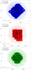 |
Fig. 1 LH (top), Boo (middle) and EN1 (bottom) fields targeted by LOFAR at 150 MHz. Light colors refer to the raw catalogs, cut at a distance from the pointing center of 0.3 of the LOFAR 150 MHz primary beam power. Darker colors refer to the final catalogs. The varying shape of their footprints highlights the regions with available optical/IR data. The areas of the optical/IR footprints are listed in Table 1. |
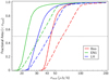 |
Fig. 2 Visibility functions of the raw (dashed lines) and final (solid lines) catalogs presented in this paper. Blue, red and green colorscorrespond to the LH, Boo and EN1 fields, respectively. The visibility functions represent the cumulative fraction of the total area of the noise map characterized by a noise lower than a given value. We caution that the total area coveredby the final catalogs is much smaller than the one covered by the raw catalogs (see Table 1). |
3.1 Visibility function of raw and final catalogs
Figure 2 shows the so-called visibility function (i.e., the cumulative fraction of the total area of the noise map characterized by noise measurements lower than a given value) for the LH (blue), Boo (red) and EN1 (green)fields. Raw and final catalogs are indicated respectively by the dashed and solid lines. We note that the visibility functions of final catalogs are significantly steeper than those of the raw catalogs. This is due to the fact that the final catalogs are mostly confined in the inner, most sensitive parts of the LOFAR fields. As a consequencethe median noise is significantly lower for final than for raw catalogs (see Table 1).
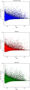 |
Fig. 3 Total to peak flux density ratio as a function of signal to noise ratio (S∕N = Speak∕σ) for both theraw (black transparent circles) and final |

3.2 Source size deconvolution
The characterization of resolved versus unresolved sources in our catalogs is important in order to correct the catalogs for the incompleteness introduced by so-called “resolution bias” (described in Sect. 4). The total flux density (Stotal) of a source can be written as:
 (1)
(1)
where Speak is the source peak flux density, θmin and θmaj are the source full-width-half-maximum (FWHM) axes, and bmin and bmaj are the restoring beam FWHM axes. In an ideal image, in the absence of noise, the total flux density of a point source is equal to its peak flux density. In real images both the total and peak flux density measurements of point sources are affected by errors. This means that not all sources with Stotal > Speak would be genuinely resolved sources. The Stotal∕Speak ratio as a function of signal-to-noise ratio (S∕N = Speak∕σ, where σ is the local rms noise), can be used to establish a statistical criterion to establish if a source is likely extended or point-like (see e.g., Prandoni et al. 2000b, 2006). In Fig. 3, the ratio of the total to peak flux densities is shown as a function of S/N for both raw and final catalogs. A lower envelope of the source distribution can be defined by the following equation:
 (2)
(2)
where A and B are two free parameters (see dashed lines in each panel of Fig. 3). As expected, going to higher S/N, measurement errors get smaller. At S∕N ≫100 the 2nd term of Eq. (2) can be neglected, and the Stotal∕Speak tends to A. In an ideal case, where radial smearing is taken care of, the ratio of the total over the peak flux density for point sources should converge to a value ofA = 1 at very highS/N. The DDFacet pipeline implements a facet dependent PSF which, for deconvolved sources, accounts for the impact of time and bandwidth smearing (Tasse 2014). However, due to imperfect calibration of the PSF across the field and/or smearing of sources due to ionospheric distortions, the value of the ratio at high signal-to-noise sources can be found to be higher than 1 and can be field-dependent (as ionospheric effects are time and spatially dependent). The values of A for the LH, Boo and EN1 field are respectively 1.15, 1.00 and 1.07 (see Table 2). This could potentially mean that the Boo field is less affected by ionospheric smearing when compared with LH and EN1. The B value also changes depending on the field, with Boo showing a lower value than LH and EN1 (see Table 2), again indicating smaller errors in the determination of source flux densities. We notice that the parameters given in Table 2 provides a good description of both raw and final catalogs. The lower envelopes can then be mirrored around the Stotal/Speak = A axis to get the upper envelopes:
 (3)
(3)
Sources lying above the upper envelopes (dashed black lines in each panel) are then considered to be truly extended or resolved sources. Sources below the upper envelopes are considered to be point sources. The fraction of resolved sources in each field is given in Table 2. In final catalogs the fraction of resolved sources vary from 24–25% (EN1 and LH) to 38% (Boo). The ~10% higher fractions observed in raw catalogs reflect the larger number of bright extended sources detected in their larger FoV. These fractions should be considered as indicative, as they depend on the criteria used to define them. Sabater et al. (2021), for instance, as part of their detailed analysis of the EN1 field, used more stringent criteria, which also include additional sources of errors for the source flux densities, and estimated that between 4 and 11% of the sources in the EN1 raw catalogs are genuinely extended (see Paper II for more details). Nevertheless, we decided to apply the same approach to all fields, and to both final and raw catalogs, to enable a consistent statistical analysis of the source size distribution in the three fields (see Sect. 4).
4 Source size distribution and resolution bias
In deriving the source counts, the completeness of the catalogs in terms of total flux density needs to be estimated. Such completeness depends on source angular sizes, since, as shown by Eq. (1), a larger source of a given total flux density will drop below the 5σ limit of a survey more easily than a smaller source of the same total flux density. This effect, called resolution bias, results from the fact that the detection of a source depends on its peak flux density. Following Prandoni et al. (2001, 2006), we can use Eq. (1) to calculate the approximate maximum deconvolved size (Θmax) a source of a given total flux density, Stotal, can have before dropping below the 5σ limit of the catalog:
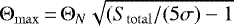 (4)
(4)
where ΘN ≡  is the geometric mean of the restoring beam axes. In our case ΘN = bmaj = bmin = 6′′.
In Fig. 4 we show the deconvolved source sizes as a function of the total flux density for both raw and final catalogs. Each panel corresponds to a different field: LH (top-left), Boo (top-right) and EN1 (bottom). Deconvolved sizes are defined as the geometric mean of the major and minor FWHM axes, except for well resolved radio galaxies, which are better described by their major axis. Deconvolved sizes of point sources are set to zero. As expected, the upper envelope of the source size distributions approximately follow the Θmax − Stotal relation (short-long-dashed line) in all fields.
Equations (1) and (3) can also be used to derive an approximate minimum intrinsic angular size (Θmin) that can be resolved reliably as a function of the source peak flux density:
 (5)
(5)
The curve representing Θmin is shown in Fig. 4 by the solid lines.
In order to quantify the fraction of sources larger than Θmax, and in turn the incompleteness affecting our catalog, we need to know the true intrinsic radio source size distribution within the flux density range probed by our survey. We start assuming the empirical integral distribution proposed by Windhorst et al. (1990) for 1.4 GHz-selected samples:
![Mathematical equation: \begin{equation*} h(>\Theta)\,{=}\,{\rm{exp}}[-\ln{2}\, (\Theta/\Theta_{\rm{med}})^{q}]\end{equation*}](/articles/aa/full_html/2021/04/aa39998-20/aa39998-20-eq7.png) (6)
(6)
where q = 0.62 and the median source size varies with the total flux density as follows:
 (7)
(7)
with k = 2′′, m = 0.3, S1.4GHz expressed in mJy. The Windhorst et al. (1990) relations are extensively used in the literature to estimate the resolution bias, either for 1.4 GHz selected samples (see e.g., Prandoni et al. 2001, 2018; Huynh et al. 2005; Hales et al. 2014a), or for surveys at other frequencies, including LOFAR HBA ones (Mahony et al. 2016; Williams et al. 2016; Retana-Montenegro et al. 2018). We converted the median size – flux density relation to 150 MHz assuming a spectral index α = −0.7. This assumption is appropriate for radio catalogs dominated by faint sub-mJy radio sources. Indeed spectral index analyses performed using shallower (S150 MHz≳1 mJy) LOFAR observations of the Boötes and LH fields, report overall median spectral index values of  and − 0.78 ± 0.24, for AGN and star-forming galaxies respectively (Boötes; Calistro Rivera et al. 2017), as well as a flattening of the spectral index going to lower flux densities, with a median value of
  at S150 MHz ~ 1−2 mJy (LH; Mahony et al. 2016).
As shown in Fig. 4 the median sizes of both raw and final catalogs (respectively indicated by filled black-bordered magenta squares and golden circles with error bars) are compared with the Windhorst et al. (1990) size – flux density relation converted to 150 MHz (long-dashed line). We see a discrepancy at intermediate flux densities (10−100 mJy), wherethe measured sizes appear in slight excess to what was predicted by Windhorst et al. (1990). We therefore decided to consider also the median size – flux density relation derived from the Tiered Radio Extragalactic Continuum Simulation (T-RECS) catalogs at 150 MHz (Bonaldi et al. 2019, dot-dashed line), which implement different size – flux density scaling relations forstar-forming galaxies and AGN. This seems to better reproduce our measured sizes at flux densities S150 MHz ~ 10−100 mJy, where extended radio galaxies (with typical sizes of hundreds of kpc) are expected to provide a significant contribution to the total radio source population. We note, however, that the afore-mentioned analysis is limited to flux densities S150 MHz≳2 mJy, while the large majority of the sources in the LoTSS Deep Fields are fainter. Most of these sources cannot be reliably deconvolved, implying that no direct information on their size distribution can be obtained. Several attempts have been made to estimate the intrinsic source sizes at sub-mJy flux densities, based on deep samples carried out over a wide range of observing frequencies (from 330 MHz to 10 GHz). Some of these works have proposed a steepening of the Windhorst et al. (1990) median size – flux density relation at sub-mJy fluxes, with m = 0.4−0.5 in the range 0.1−1 mJy (Richards 2000; Bondi et al. 2003, 2008; Smolčić et al. 2017). A smooth transition from a flatter to a steeper relation at sub-mJy flux densities could again be justified by a smooth transition from a flux regime dominated by extended radio galaxies (S ≫ 1 mJy) to a flux regime dominated by radio sources triggered by star-formation (or by composite SF/AGN emission), confined within the host galaxy.
In order to establish which size–flux density relation would best quantify the incompleteness of our catalogs we have decided to include in our analysis the results from other deep surveys. Figure 5 shows the existing measurements of (median) source sizes in various flux density bins for a number of surveys (different colors/symbols refer to different observing frequencies). Also shown are the median sizes derived by combining together the three LoTSS fields (raw and final catalogs, respectively indicated by filled black-bordered magenta squares and golden circles). To make the comparison meaningful, all flux densities referring to a different observing frequency have been converted to 1.4 GHz, assuming α = −0.7. Also shown are various size – flux density relations: the ones proposed by Bonaldi et al. (2019, converted to 1.4 GHz) and Windhorst et al. (1990) (dot-dashed and long-dashed lines respectively), and some modifications of the latter. The short dashed lines show the ones obtained by rescaling the Windhorst et al. (1990) relation by 1.5 × and 2 × (i.e., assuming k = 3 and k = 4 in Eq. (7)), while the dotted line assumes a smooth transition between m = 0.3 and m = 0.5 going from mJy to sub-mJy flux densities, i.e.,:
 (8)
(8)
with S1.4GHz expressed in mJy. Focusing on the sub-mJy regime, it is clear that both the Windhorst et al. (1990) and the steeper m(S) relations are consistent with the observed sizes, especially when considering only the 1.4 GHz surveys (black filled triangles). Surveys undertaken at higher frequencies seem to point toward the steeper relation, but these samples may be biased toward a flatter spectrum population, resulting in an over-estimation of the flux densities once converted to 1.4 GHz assuming a too steep spectral index. We also caution that higher frequency surveys more easily miss extended flux, and resolution bias issues can indeed mimic a steepening of source median sizes getting close to the flux limit of a radio survey. At larger flux densities (S1.4GHz≳1 mJy) the median sizes are observed to lie between the Windhorst et al. (1990) relations described by k = 2 and k = 4, with a tendency for larger sizes going to lower frequency. Indeed some analyses of source counts with shallower LOFAR surveys in the LH and Boo fields claimed in the past a better consistency with a k = 4 Windhorst et al. (1990) median size – flux scaling relation (Mahony et al. 2016; Retana-Montenegro et al. 2018). It is interesting to note, however, that the LoTSS final catalogs are characterized by smaller median sizes than the raw catalogs at their faint end (S1.4GHz≲5 mJy), indicating that confusion significantly affects the measured sizes of the faintest sources, and that a significant number of faint sources were deblended. On the other hand, the final catalogs tend to be characterized by larger sizes at the bright end (S1.4GHz≳100 mJy), likely as a consequence of the association of multiple components into single sources, after visual inspection of the radio/optical images (see Sect 3). After accounting for these effects, LoTSS median sizes (golden filled circles) are consistent with the Windhorst et al. (1990) k = 2 size – flux relation up to S1.4GHz ~ 2 mJy. Then they smoothly increase and become consistent with the Bonaldi et al. (2019) relation at S1.4GHz≳10 mJy. At S1.4GHz≳100 mJy the LoTSS source median sizes show large uncertainties. At these large flux densities also the Bonaldi et al. (2019) relation is poorly determined, being based on a simulated catalog covering a similar area to the one covered by the LOFAR deep fields (25 deg2). It is interesting to note, however, that both are consistent with the Windhorst et al. (1990) relation. Based on all the above considerations, a good description of the observed median sizes can be obtained by the following analytical form, which assumes the Windhorst et al. (1990) relation with a varying k = k(S), i.e.,:
 (9)
(9)
where S1.4GHz is expressed inmJy (see solid line in Fig. 5).
Another important consistency check regards the angular size distribution of the sources. Figure 6 shows the cumulative size distributions of the final catalogs combined together, in four flux density bins (yellow solid lines). Such distributions can be considered reliable only down to a flux-dependent minimum intrinsic size (see vertical gray lines), below which most of the sources cannot be reliably deconvolved and they are conventionally assigned Θ = 0. The observed distributions are compared with various realizations of the cumulative distribution function described by Eq. (6), obtained by varying either the function exponent q (left and right columns respectively) or the assumed median size – flux relations (see various black lines).The original function proposed by Windhorst et al. (1990) (Eq. (6) with q = 0.62, see left column) does provide a good approximation of the observed distributions, when assuming the original Θmed − S relation described by Eq. (7), only at flux densities S150 MHz≳10 mJy (see long-dashed lines). This is perhaps not surprising considering that this relation was calibrated at 1.4 GHz down to a few mJy fluxes. At the lowest flux densities (S150 MHz≲1 mJy) we need to assume a steepening of the parameter m (see Eq. (8)), to get a good match with observations (dotted line in the top left panel). This is consistent with what proposed for higher frequency deep surveys (as discussed earlier in this section). At intermediate fluxes (S150 MHz ~ 1−10) mJy, on the other hand, none of the discussed median size – flux relations can reproduce the observed size distribution (see second-row panel on the left). It is interesting to note, however, that if we assume a steeper exponent for the distribution function described by Eq. (7) (i.e., q = 0.80), we get a very good match with observations at all fluxes, when assuming a flux-dependent scaling factor (k = k(S); see Eq. (9)) for the Windhorst et al. (1990) median size – flux relation (black solid lines on the right). The median sizes derived from the T-RECS simulated catalogs (Bonaldi et al. 2019) also provide good results for q = 0.80 (dot-dashed lines on the right), except again at intermediate fluxes (S150 MHz ~ 1−10), where they show strong discrepancies with observations also in Fig. 5. This seems to indicate that the number density of extended radio galaxies in this flux density range is over-estimated in the T-RECS simulated catalogs.
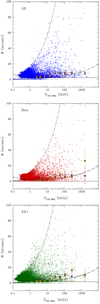 |
Fig. 4 Source intrinsic (deconvolved) angular sizes as a function of the measured 150 MHz total flux densities. Deconvolved sizes are defined as the geometric mean of the major and minor FWHM axes, except for well resolved radiogalaxies, which are better described by their major axis. Deconvolved sizes of point sources are set to zero. Raw (▪) and final ( |

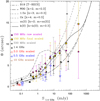 |
Fig. 5 Source median angular size vs. 1.4 GHz total flux density, as estimated in some of the deepest radio samples available so far. Different colors/symbols correspond to different observing frequencies: 330 MHz (gray filled diamonds – Owen et al. 2009); 1.4 GHz (black filled triangles – Richards 2000; Bondi et al. 2003, 2008; Muxlow et al. 2005; Prandoni et al. 2018); 3 GHz (red empty squares – Bondi et al. 2018; Cotton et al. 2018); 5.5 GHz (blue stars – Prandoni et al. 2006; Guidetti et al. 2017); 10 GHz (brown asteriscs – Murphy et al. 2017). Also shown are the median sizes measured in our raw and final catalogs (150 MHz), combined together (filled black-bordered magenta squares and golden circles). We note that Guidetti et al. (2017) gives different median sizes for the AGN and star-forming galaxy subpopulations. The latter population is indicated as a circled blue star in the figure. All flux densities have been converted to 1.4 GHz, assuming a spectral index α = − 0.7. Various median size – flux density relations are shown for comparison: the ones proposed by Bonaldi et al. (2019) and Windhorst et al. (1990) (dot-dashed and long-dashed lines respectively), and some revised versions of the latter. The short dashed lines show the relations obtained by rescaling the Windhorst et al. (1990) relation by 1.5 × and 2 × (i.e., assuming k = 3 and k = 4 in Eq. (7)); the dotted line assumes a smooth transition between m = 0.3 and m = 0.5 going from mJy to sub-mJy flux densities,a s described by Eq. (8); the solid line assumes a value of k varying with flux density according to Eq. (9) (see text for more details). |
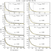 |
Fig. 6 Source size cumulative distribution of final catalogs (yellow solid line) in four 150 MHz flux density bins (top to bottom). The vertical gray lines in all panels provides an approximate indication of the minimum intrinsic angular size to which the observed distributions can be considered reliable (most of the sources below this line cannot be reliably deconvolved and they are conventionally assigned Θ = 0). Also shown for comparison are various realizations of the cumulative distribution function described by Eq. (6). The two columns correspond to two different values for the function exponent q: the original one proposed by Windhorst et al. (1990) (q = 0.62) on the left, and a steeper one (q = 0.80) on the right. In addition we also vary the median size – flux relation. In particular we assume the original Windhorst et al. (1990) relation (black long-dashed line), the revised versions with flux-dependent m and k parameters, as described by Eqs. (8) and (9) (black dotted and solid lines respectively) and the one describing the T-RECS catalogs (Bonaldi et al. 2019; black dot-dashed line). All such realizations are shown on the left; on the right we only show the realizations obtained using the Bonaldi et al. (2019) and the revised Windhorst et al. (1990) k = k(S) relations. |
Correction for resolution bias
The correction factor c that needs to be applied to the source counts to account for the resolution bias can be defined as (Prandoni et al. 2001):
![Mathematical equation: \begin{equation*} c\,{=}\, 1/[1-h(>\Theta_{\rm{lim}})] \end{equation*}](/articles/aa/full_html/2021/04/aa39998-20/aa39998-20-eq14.png) (10)
(10)
where h(> Θlim) takes the form of the integral of the angular size distribution proposed by Windhorst et al. (1990, see Eq. (6)), and Θlim is the limiting angular size above which the catalogs are expected to be incomplete. Following Prandoni et al. (2001), this is defined as:
![Mathematical equation: \begin{equation*} \Theta_{\rm{lim}}\,{=}\,\rm{max}[\Theta_{\rm{min}},\Theta_{\rm{max}}] \end{equation*}](/articles/aa/full_html/2021/04/aa39998-20/aa39998-20-eq15.png) (11)
(11)
where Θmax and Θmin are as defined in Eqs. (4) and (5) respectively. We notice that Θlim is always equal to Θmax, except for the lowest flux bins, where Θmax becomes unphysical (i.e., tends to zero). Θmin accounts for the effect of having a finite restoring beam size (that is Θlim > 0 at the survey limit) and a deconvolution efficiency which varies with the source peak flux density (see Prandoni et al. 2001 for more details).
Figure 7 (left panel) shows the correction factor derived assuming the median size – flux relations discussed above, combined with appropriate values of the q exponent in Eq. (6), based on our analysis of the source size distribution (see Fig. 6 and related discussion). A caveat to keep in mind is that the resolution bias correction does depend on both the source flux density and the noise value at the source position (and/or the source signal-to-noise ratio; see Eqs. (4) and (5)). The corrections presented inFig. 7 (left panel) account for local and radial variations of the noise through empirical relations between source flux and local noise or signal-to-noise ratio, specifically derived for each field. Such relations describe average trends only, and hence the corrections presented here should be considered as indicative. The corrections effectively applied to the counts are based on the actual source flux density, noise and signal-to-noise ratio distributions. It is interesting to note, however, that, as a consequence of radially-increasing noise (and/or limited dynamic range around bright radio sources), the correction factor c does not necessarily converge to 1 at large flux densities. As shown in Fig. 7, in the masked regions of our fields this only happens when assuming the shallower integral distribution function (q = 0.62). For the steeper one (q = 0.80), the expected number density of very extended sources is small, and resolution bias effects become negligible at S150 MHz≳500 mJy.
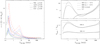 |
Fig. 7 Left: flux-dependent correction to be applied to source counts to account for incompleteness due to resolution bias, for four median size - flux relations: the one derived from the simulated T-RECS catalogs (Bonaldi et al. 2019; dot-dashed lines), the one proposed by Windhorst et al. (1990, long-dashed lines), the revised version with m = m(S), which betterdescribe source sizes at 1.4 GHz sub-mJy fluxes (see Eq. (8), dotted lines), and the revised version with k = k(S) proposed by us (Eq. (9), solid lines). We also vary the q exponent of the integral distribution function. Based on our analysis of the source size distribution (see Fig. 6 and related discussion), we assume the original value proposed by Windhorst et al. (1990, q = 0.62) for the Windhorst et al. (1990) median size – flux relation and for the revised version with m = m(S). We assume asteeper q = 0.80 for the revised version with k = k(S) and for the Bonaldi et al. (2019) relation (see legenda). Different colors refer to different fields: LH (blue), Boo (red), EN1 (green). The corrections account for noise variations in the masked images through an empirical relation between source flux and source signal-to-noise ratio, calibrated for each field (we assume here the median noise of the masked images; see last column of Table 1). Right: Eddington bias for different underlying number-count distributions, as illustrated in the top panel: source counts’ slope (γ; d N∕d S ~ S−γ) derived from the sixth-order polynomial fit proposed at 1.4 GHz by (a) Hopkins et al. (2003; dot-dashed line) and (b) Bondi et al. (2008; dashed line), both converted to 150 MHz assuming a spectral index α = − 0.7; we also show a revised version of the Bondi et al. (2008) fit, which assumes a constant Euclidean slope (γ = 2.5) from 2 mJy all the way down to 0.1 mJy (dotted line). The polynomial fit proposed by Intema et al. (2017) at 150 MHz and valid only for the bright end of the counts is also shown for reference (solid line). The flux boosting (Smeas ∕Strue) corresponding to the three cases illustrated above is shown in the bottom panel for two different source signal-to-noise ratios: S∕N = 5 and S∕N = 10. |
5 Eddington bias
While correcting for resolution bias is important to account for missed resolved sources, Eddington bias (Eddington 1913, 1940) should be taken into account to get an unbiased census of unresolved sources. Due to random measurement errors the measured peak flux densities will be redistributed around their true value. In presence of a source population which follows a nonuniform flux distribution, this will result in a redistribution of sources between number-count flux density bins. The way the sources are redistributed depends on the slope of source counts. If the source number density increases with decreasing flux, the flux densities tend to be boosted and the probability to detect a source below the detection threshold is higher than the probability to miss a source above the threshold, artificially boosting the detection fraction. As a consequence the catalog incompleteness at the detection threshold is also biased.
There are two main approaches to correct for Eddington bias, both requiring an assumption about the true underlying source counts distribution (see Hales et al. 2014a for a full discussion): one can build the source counts using the boosted flux densities and then apply a correction to each flux density bin, or one can correct the source flux densities, before deriving the counts. As demonstrated by Hales et al. (2014b) the two approaches give very similar and consistent results, and we decided to follow the latter approach. A maximum likelihood solution for the true source flux density can be defined as follows (see Hales et al. 2014a and references therein):
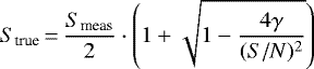 (12)
(12)
where γ = γ(S) is the slope of the counts at the given flux density (dN∕dS ~ S−γ), and S/N is the source signal-to-noise ratio. The slope of the counts can be modeled from empirical polynomial fits of the observed counts:
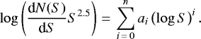 (13)
(13)
It is then easy to demonstrate that:
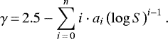 (14)
(14)
In order to derive γ we can use one of the several counts’ fits available in the literature. Intema et al. (2017) derived a fifth-order polynomial fit which describes the 150 MHz normalized counts of the TIFR GMRT Sky Survey (TGSS-ADR1), but this fit is only valid down to a flux limit of 5 mJy. The deepest fits available in the literature have been obtained at 1.4 GHz. We start by exploring the sixth-order (n = 6) polynomial fits obtainedby Hopkins et al. (2003) and Bondi et al. (2008) for 1.4 GHz normalized source counts (converted to 150 MHz using α = −0.78). The two cases are illustrated in the top right panel of Fig. 7 (dot-dashed and dashed lines respectively), where the derived counts’ slope is shown. Both cases are consistent with the Intema et al. (2017) 150 MHz fit (indicated by the solid line) at bright flux densities (S > 100 mJy), while significant discrepancies are observed at fainter fluxes, where the deeper 1.4 GHz fits better describe the well-known flattening of the normalized counts. Both the 1.4 GHz fits show an increasing slope below 10 mJy, reaching a maximum around 1 mJy. This maximum is more pronounced in the case of Bondi et al. (2008), and is consistent with an Euclidean slope of γ ~ 2.5. At S < 1 mJy both slopes show a rapid drop. The reality and strength of this drop is unclear, as this is the flux regime where the fits are less reliably constrained. We then explore a third case, i.e., a modification of the Bondi et al. (2008) fit, which assumes a constant Euclidean slope at flux densities S < 2 mJy. This represents an extreme scenario, which however might be favored by the recent 150 MHz source counts modeling proposed by Bonaldi et al. (2019), that indicates a flatter slope in the flux range 0.1−1 mJy. This last case is illustrated by the dotted line in Fig. 7 (top right panel). The flux density boosting expected for the three aforementioned scenarios is illustrated in the bottom right panel of Fig. 7 for two signal-to-noise ratio values, S∕N = 5 and S∕N = 10.
Once the point source flux densities are corrected for Eddington bias, we can obtain an estimate of the catalog incompleteness at the detection threshold through the use of Gaussian Error Functions (ERF).
6 Differential source counts
The differential source counts, normalized to a non-evolving Euclidean model, obtained from the LoTSS Deep Fields are shown in Fig. 8, together with other count determinations obtained in the same fields from previous low-frequency surveys (see legend). The top and bottom panels refer to counts derived from the raw and final catalogs, respectively (see filled boxes). The source counts obtained from the final catalogs are reported in tabular form in the appendix (Tables A.1–A.3, for LH, Boo and EN1 fields respectively), and are also shown in Fig. 10, where they are compared to counts extrapolated from higher frequencies. In deriving the counts we applied a ‘fiducial’ model for the systematic corrections described in Sects. 4 and 5. Specifically we assumed the Windhorst et al. (1990) size – flux relation with k = k(S) (Eq. (9)), in combinationwith a ‘steep’ (q = 0.80 in Eq. (6)) integral size distribution, to estimate the resolution bias, and we assumed the Bondi et al. (2008) source counts best fit to estimate the Eddington bias. The uncertainties associated with such assumptions are factored into systematic error terms (see Sys− and Sys+ columns in the counts’ tables), that are defined as the maximum discrepancy between the ‘fiducial’ counts and those obtained assuming the other discussed models (shown in Fig. 7). Also shown in Fig. 8 are the counts obtained from the three LoTSS fields before applying the corrections for resolution and Eddington bias (empty boxes). As expected such corrections are only relevant for the lowest flux density bins. We cut the source counts at a threshold of ~ 7σmed, where systematic errors dominate over Poissonian (calculated following Gehrels 1986) by factors ~ 5−10.
The normalized 150 MHz source counts derived from the three LoTSS Deep Fields are in broad agreement with each other, and show the well known flattening at S≲ few mJy. The observed field-to-field variations for the counts derived from the final catalogs are typically on the order of a few percent at sub-mJy fluxes, and of 5–10% at flux densities 1− 10 mJy, with EN1 showing somewhat larger deviations (up to 15–20% in some flux density bins). This is consistent with expectations from sample variance for surveys covering areas of 5−10 deg2 (Heywood et al. 2013; Prandoni et al. 2018). We notice that all of the other 150 MHz counts shown in Fig. 8 come from previous shallower LOFAR observations, but the catalogs did not go through the source association and deblending post-processing described in Sect. 3. This explains why determination of previous source counts are more in line with those we obtained from raw catalogs (see top panel of Fig. 8). The largest discrepancies are observed in the Boo field with the counts by Retana-Montenegro et al. (2018). The systematically higher counts that we obtain at sub-mJy flux densities may be the result of the new calibration and imaging pipeline, that produces higher fidelity, higher dynamic range images (Paper I). Another source of systematic differences may be a residual offset in the absolute flux scale.
When comparing the source counts derived from raw and final catalogs (top and bottom panels of Fig. 8), we notice a very interesting feature: the latter show a much more pronounced drop at flux densities around a few mJy, which results in a more prominent ‘bump’ in the sub-mJy regime. For a more quantitative analysis of this feature we have combined the sources in the three fields and produced a combined version of the source counts. This allows us to smooth out the aforementioned field-to-field variations, as well as reduce the scatter at bright flux densities, where Poissonian errors dominate. The combined counts derived from raw and final catalogs are shown in Fig. 9 and listed in Table 3. We notice that in this case we included LH and Boo sources down to a 5σ flux density limit, to increase the statistics available in the first two flux density bins. From the comparison of the raw and final counts we see that the latter are systematically lower by a factor 5− 15% in the range S ~1−10 mJy. This deficiency appears to be counterbalanced by an 8−16% excess at flux densities 0.2−0.6 mJy. This form of compensation is likely the result of source deblending (see Sect. 3 for more details). Indeed, for each field we have ~1000 s deblended sources (see Paper II), and deblending is mostly effective at the faint end of the counts, where it contributes to the increase of the number of the sources, through the splitting of confused (brighter) sources into several fainter ones. Artifact removal, on the other hand, has probably a limited effect. Artifacts mostly affect the flux density range 2− 20 mJy9, but only <100 sources per field are confirmed as such (see Paper II). The fact that source cataloguing processes can significantly affect the derived number counts is well known. Significant discrepancies are observed, for instance, when comparing counts derived from source catalogs with those directly obtained from Gaussian components (see e.g., Hopkins et al. 2003). While PyBDSF creates a source catalog, our association and deblending procedure aims at further combining Gaussian components together (association) or splitting them into several independent sources (deblending), hence modifying the source statistics and flux distribution of the original PyBDSF catalog.
As a final remark we note that none of the best fits from previous source counts (shown in Fig. 8) provide a good description of the pronounced ‘drop and bump’ feature that we observe at 150 MHz. We have therefore derived a new fit that better matches the faint end of the 150 MHz counts derived from our final catalogs. The slope of the counts is modeled by a 7th order polynomial function defined in the log-log space, according to Eq. (13) (see Sect. 5 for more details). To better constrain the bright end of the counts, where the LoTSS Deep Fields provide poor statistics, we have included the counts derived from the TGSS-ADR1 (Intema et al. 2017), up to a flux density of 10 Jy (beyond that the TGSS-ADR1 itself is affected by poor statistics). The resulting coefficient values and their uncertainties are listed in Table 4; the fitted curve is shown in Fig. 9.
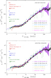 |
Fig. 8 Normalized 150 MHz differential source counts in the three LoTSS Deep Fields, as derived from raw (top) and final (bottom) catalogs (filled squares). Error bars correspond to the quadratic sum of Poisson and systematic errors. Also shown are the counts obtained without applying the corrections discussed in Sects. 4 and 5 (empty squares). The counts are derived by using total flux densities for both point and extended sources. In both figures, Wilman et al. (2008), Bonaldi et al. (2019) and Mancuso et al. (2017) 150 MHz models are shown for comparison, as well as other existing 150 MHz counts’ determinations in the same fields (see legend). Since published 150 MHz counts are missing for EN1, we show a recent determination obtained at 610 MHz (Ocran et al. 2020) and rescaled to 150 MHz, assuming α = − 0.7. Also shown are the counts’ best fits discussed in Sect. 5. |
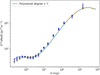 |
Fig. 9 150 MHz Euclidean normalized differential source counts as derived from the LoTSS Deep Fields: raw catalog are indicated by transparent black circles and final catalog by blue crosses. Also shown are the counts obtained from the TGSS-ADR1 (Intema et al. 2017, orange filled circles), which better describe the counts’ bright end. Over-plotted is the best fit obtained by modeling the counts in the log–log space with a 7th order polynomial function, according to Eq. (13) (see Table 4 for the values of the best-fit coefficients and associated errors). |
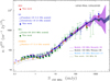 |
Fig. 10 Normalized 150 MHz differential source counts in the three LoTSS Deep Fields, as derived from final catalogs (filled squares), together with their best fit (gray solid line). They are compared to counts derived from higher frequencies surveys (see legend), and rescaled to 150 MHz by assuming α = − 0.7. Error bars correspond to the quadratic sum of Poisson and systematic errors. Also shown are the Wilman et al. (2008), Bonaldi et al. (2019) and Mancuso et al. (2017) 150 MHz models. The counts are derived by using total flux densities for both point and extended sources. |
6.1 Qualitative comparison with higher frequency counts
Our source counts are the deepest available at 150 MHz. Their faint end can therefore only be probed against counts obtained from higher frequency surveys of similar depth. In Fig. 10 we show the normalized differential counts in the three LoTSS Deep Fields, as derived from final catalogs, together with counts derived from higher frequencies surveys over the same regions of the sky, and rescaled to 150 MHz by assuming α = −0.7. We also add theCOSMOS 3GHz Large project (Smolčić et al. 2017), which provides the deepest counts to date, over a degree-scale field. None of the higher frequency counts show the pronounced ‘drop’ at mJy flux densities, that we observe at 150 MHz. The only exception is COSMOS, which is in agreement with our 150 MHz counts at S≳1 mJy, but falls below them at lower flux densities. We note that sample variance can in principle explain variations ≳15− 25% in the range 1− 10 mJy for surveys covering areas ≲2 deg2 (Heywood et al. 2013), like COSMOS and the ones by Ocran et al. (2020) and Vernstrom et al. (2016) in EN1 and LH respectively,but can hardly justify the observed discrepancies with Prandoni et al. (2018) sample, which covers more than half (~ 6.6 deg2) of the LoTSS LH field. In addition, sample variance is expected to be on the order of 5–10% at sub-mJy fluxes for a sample like COSMOS, i.e., smaller than what observed. It is then likely that survey systematics additionally contribute to the observed field-to-field variations. In this respect we note that the excess at mJy flux densities is significantly mitigated when comparing the higher frequency counts to the LoTSS ones derived from raw catalogs (see Ocran et al. 2020 counts in top panel of Fig. 8), indicating that the catalog post-processing undertaken for the LoTSS deep fields did play a role here. Indeed we could count on very complete identification rates (≳97% of radio sources havean optical/IR counterpart), enabling a very accurate process of association, deblending and artifact removal. This is not true for other samples which went through similar procedures, like the Prandoni et al. (2018) sample (identification rate ~ 80% down to S1.4 GHz = 0.12 mJy) or the Ocran et al. (2020) sample (identification rate ~90%). On the other hand, COSMOS counts may suffer from flux losses at their faintest end, being derived from a higher frequency (3 GHz), higher (sub-arcsec) resolution survey. Another source of systematics may be the extrapolation of the higher frequency counts to 150 MHz, which is sensitive to the assumed spectral index. In particular, adopting the same spectral index value for all the sources may not be appropriate. There are indeed indications that the spectral index may flatten at mJy/sub-mJy regimes, due to the emergence of a population of low power, core dominated AGN (e.g., Prandoni et al. 2006; Whittam et al. 2013) and re-steepen again at μJy levels, where star-forming galaxies become dominant (e.g., Owen et al. 2009).
150 MHz normalized differential radio-source counts as derived from combining the raw and final catalogs of the three LoTSS Deep Fields.
6.2 Qualitative comparison with models
The source counts derived from the LoTSS Deep Fields provide unprecedented observational constraints to the shape of the source counts at 150 MHz sub-mJy flux densities. As such they can be compared with counts predictions based on existing evolutionary models of radio source populations. A comprehensive comparison with models is beyond the scope of this paper, and will be the subject of forthcoming papers, where counts and luminosity functions will be presented and discussed for various radio source populations. Here we only provide some first qualitative considerations.
In Figs. 8 and 10 we compare the LoTSS source counts to the 150 MHz determinations derived from the Wilman et al. (2008) and Bonaldi et al. (2019) simulated catalogs10 (black and dark violet shaded curves, respectively), as well as from Mancuso et al. (2017) models (light blue curve). We notice that the Bonaldi et al. (2019) and Wilman et al. (2008) source counts are very similar at the bright end and better reproduce the observations than Mancuso et al. (2017). On the other hand, Bonaldi et al. (2019) and Mancuso et al. (2017) counts are very similar at the faint end, and in better agreement with the observations than Wilman et al. (2008). Nevertheless, neither Bonaldi et al. (2019) nor Mancuso et al. (2017) can reproduce the pronounced bump at sub-mJy flux densities, observed in the counts derived from final catalogs (see Fig. 8, bottom panel, or Fig. 10). In addition all models appear to over-estimate the counts derived from our final catalogs at intermediate flux densities (S ~ 2−20 mJy). An over-prediction of the observed counts over T-RECS and Wilman et al. (2008) simulations in the flux density range 3− 12 mJy was also noticed by Siewert et al. (2020) in their analysis of the HETDEX field of LoTSS-DR1 (Shimwell et al. 2017, 2019).
In an attempt to better understand where the evolutionary models may fail, we compare the observed source redshift distribution (using redshifts from Paper IV) with those of the Bonaldi et al. (2019) simulated catalog. We restrict this comparison to the EN1 field, as it is the deepest and has the most complete optical coverage among the three LoTSS Deep Fields. We limit our analysis to the flux density range 0.25 mJy ≤ S150 ≤ 20 mJy. At lower flux densities the effects of the visibility function and of incompleteness cannot be neglected anymore; at larger flux densities the available source statistics is very sparse. In the flux density regime under consideration, we have 14, 916 sources; 14 432 of them (97%) have measured redshifts (91% photometric and 9% spectroscopic, see Paper IV). 3% of the sources do not have redshift estimates, and are not included in the analysis. We believe the effect of neglecting these sources does not alter the main results of our analysis. Photometric redshifts can be considered robust up to z = 1.5 for galaxies (σNMAD = 1.48 × median(|Δz|∕(1 + zspec)) = 0.02), and up to z = 4 for AGN (σNMAD = 0.064; we refer to Paper IV for more details).
In Fig. 11 we show the redshift distributions of the sources in the EN1 field (solid black lines) for various flux density bins. These distributions are compared with the simulated distributions based on Bonaldi et al. (2019) evolutionary models (blue histogram bars). In the flux density bins spanning from 0.25 to 0.75 mJy we see a clear deficiency of the simulated sources, in agreement with the observed excess in the counts. This deficiency is mainly associated with sources at z < 1. The fact that the source counts’ excess is observed in all of the LoTSS fields (see e.g., Fig. 8) seems to rule out the case this is due to cosmic variance. We cannot exclude however, that the clustering properties assumed in the simulation may play a role in producing the observed discrepancy11. At larger flux densities (S≳1 mJy), we see an opposite trend, i.e., there is an excess of simulated sources with respect to observations. This is again consistent with the deficiency observed in our counts in the range 2− 20 mJy. This excess is associated with intermediate redshift (1 < z < 2) sources, andappears to be mostly due to an excess of AGN in the simulated catalog, at least at flux densities larger than a few mJy. We note that both the source excess at sub-mJy fluxes and the AGN deficiency at the brightest fluxes are observed at redshifts where the involved populations (galaxies and AGN in the former, AGN only in the latter) have robust photometric redshift estimates.
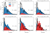 |
Fig. 11 Redshift distribution of the simulated sources in Bonaldi et al. (2019) catalog: the blue histogram corresponds to the total number of sources; the red histogram corresponds to the AGN component only. The solid black line shows the redshift distribution of the sources in the EN1 field. For a proper comparison the y-axis represents the source density in each catalog. Each panel corresponds to a different flux density bin, increasing from left to right and from top to bottom. Redshift bins range from Δz = 0.14 to Δz = 0.22 from the faintest to the brightest flux bin, i.e., they are larger than the estimated photometric redshift scatter by a factor 2− 3 for AGN andby a factor ≥7 for galaxies. We caution that the EN1 redshift distributions are reliable only up to z ~ 1.5 for galaxies and up to z ~ 4 for AGN. |
7 Conclusions
In this paper, we have presented the source number counts derived from the LoTSS Deep Fields: the Lockman Hole (LH), the Boötes (Boo) and the Elais-N1 (EN1). With central rms noise levels of 22, 33, 17 μJy beam−1 the LH, Boo and EN1 fields are the deepest obtained so far at 150 MHz, allowing us to get unprecedented observational constraints to the shape of the source counts at 150 MHz sub-mJy flux densities. We compared the source counts derived from the LoTSS deep fields with other existing source-counts determinations from low- and high- frequency radio surveys, and state-of-the-art evolutionarymodels. Our counts are in broad agreement with those from the literature, and show the well known upturn at ≲1 mJy, which indicates the emergence of the star forming galaxy population. More interestingly, our counts show for the first time a very pronounced drop around S ~ 2 mJy, which results in a prominent ‘bump’ at sub-mJy flux densities. Such a ‘drop and bump’ feature was not observed in previous counts’ determinations (neither at 150 MHz nor at higher frequency). While sample variance can play a role in explaining the observed discrepancies, we believe this is mostly the result of a careful analysis aimed at deblending confused sources from the radio source catalogs (see Paper II). Our counts cannot be fully reproduced by any of the existing evolutionary models. From a qualitative comparison with Bonaldi et al. (2019) simulated catalogs, we find that the sub-mJy ‘bump’ appears to be associated with an excess of low-redshift (z < 1) galaxies and/or AGN, while the drop at mJy flux densities seems to be due to a deficiency of AGN at redshifts 1 < z < 2. A more in-depth investigation of these preliminary results will be the subject of forthcoming papers, based on more comprehensive comparisons with models.
Acknowledgements
We thank the anonymous referee for constructive suggestions that allowed us to improve our draft. This paper is based (in part) on data obtained with the International LOFAR Telescope (ILT) under project code LC3_008. LOFAR (van Haarlem et al. 2013a) is the Low Frequency Array designed and constructed by ASTRON. It has observing, data processing, and data storage facilities in several countries, that are owned by various parties (each with their own funding sources), and that are collectively operated by the ILT foundation under a joint scientific policy. The ILT resources have benefitted from the following recent major funding sources: CNRS-INSU, Observatoire de Paris and Université d’Orléans, France; BMBF, MIWF-NRW, MPG, Germany; Science Foundation Ireland (SFI), Department of Business, Enterprise and Innovation (DBEI), Ireland; NWO, The Netherlands; The Science and Technology Facilities Council, UK ; Istituto Nazionale di Astrofisica (INAF), Italy. This paper is based on the data obtained with the International LOFAR Telescope (ILT). The Leiden LOFAR team acknowledge support from the ERC Advanced Investigator programme NewClusters 321271 and the VIDI research programme with project number 639.042.729, which is financed by the Netherlands Organisation for Scientific Research (NWO). A.D. acknowledges support by the BMBF Verbundforschung under the grant 05A17STA. The Jülich LOFAR Long Term Archive and the German LOFAR network are both coordinated and operated by the Jülich Supercomputing Centre (JSC), and computing resources on the supercomputer JUWELS at JSC were provided by the Gauss Centre for supercomputing e.V. (grant CHTB00) through the John von Neumann Institute for Computing (NIC). T.M.S. and D.J.S. acknowledge the Research Training Group 1620 ‘Models of Gravity’, supported by Deutsche Forschungsgemeinschaft (DFG) and support of the German Federal Ministry for Science and Research BMBF-Verbundforschungsprojekt D-LOFAR IV (grant number 05A17PBA). P.N.B. is grateful for support from the UK STFC via grant ST/R000972/1. M.J.H. acknowledges support from the UK Science and Technology Facilities Council (ST/R000905/1). I.P. and M.B. acknowledge support from INAF under PRIN SKA/CTA “FORECaST” and PRIN MAIN STREAM “SAuROS” projects, as well as from the Ministero degli Affari Esteri e della Cooperazione Internazionale - Direzione Generale per la Promozione del Sistema Paese Progetto di Grande Rilevanza ZA18GR02. J.S. is grateful for support from the UK STFC via grant ST/R000972/1. M.J.J. acknowledges support from the UK Science and Technology Facilities Council [ST/N000919/1] and the Oxford Hintze Centre for Astrophysical Surveys which is funded through generous support from the Hintze Family Charitable Foundation. R.K. acknowledges support from the Science and Technology Facilities Council (STFC) through an STFC studentship via grant ST/R504737/1. W.L.W. acknowledges support from the ERC Advanced Investigator programme NewClusters 321271. W.L.W. also acknowledges support from the CAS-NWO programme for radio astronomy with project number 629.001.024, which is financed by the Netherlands Organisation for Scientific Research (NWO). K.L.E. acknowledges financial support from the Dutch Science Organization (NWO) through TOP grant 614.001.351. This research made use of APLpy, an open-source plotting package for Python hosted at http://aplpy.github.com.
Appendix A LoTSS Deep Fields - Counts’ tables
150 MHz normalized differential radio-source counts as derived from the Lockman Hole final catalogs.
150 MHz normalized differential radio-source counts as derived from the Boötes final catalogs.
150 MHz normalized differential radio-source counts as derived from the ELAIS-N1 final catalogs.
References
- Baldwin, J. E., Boysen, R. C., Hales, S. E. G., et al. 1985, MNRAS, 217, 717 [NASA ADS] [Google Scholar]
- Becker, R. H., White, R. L., & Helfand, D. J. 1995, ApJ, 450, 559 [NASA ADS] [CrossRef] [Google Scholar]
- Bennett, A. S. 1962, MNRAS, 68, 163 [Google Scholar]
- Bonaldi, A., Bonato, M., Galluzzi, V., et al. 2019, MNRAS, 482, 2 [NASA ADS] [CrossRef] [Google Scholar]
- Bonato, M., Negrello, M., Mancuso, C., et al. 2017, MNRAS, 469, 1912 [Google Scholar]
- Bonato, M., Prandoni, I., De Zotti, G., et al. 2021, MNRAS, 500, 22 [Google Scholar]
- Bondi, M., Ciliegi, P., Zamorani, G., et al. 2003, A&A, 403, 857 [NASA ADS] [CrossRef] [EDP Sciences] [Google Scholar]
- Bondi, M., Ciliegi, P., Schinnerer, E., et al. 2008, ApJ, 681, 1129 [NASA ADS] [CrossRef] [Google Scholar]
- Bondi, M., Zamorani, G., Ciliegi, P., et al. 2018, A&A, 618, L8 [NASA ADS] [CrossRef] [EDP Sciences] [Google Scholar]
- Bonzini, M., Padovani, P., Mainieri, V., et al. 2013, MNRAS, 436, 3759 [NASA ADS] [CrossRef] [Google Scholar]
- Bonzini, M., Mainieri, V., Padovani, P., et al. 2015, MNRAS, 453, 1079 [NASA ADS] [CrossRef] [Google Scholar]
- Brunner, H., Cappelluti, N., Hasinger, G., et al. 2008, A&A, 479, 283 [NASA ADS] [CrossRef] [EDP Sciences] [Google Scholar]
- Calistro Rivera, G., Williams, W. L., Hardcastle, M. J., et al. 2017, MNRAS, 469, 3468 [NASA ADS] [CrossRef] [Google Scholar]
- Chambers, K. C., Magnier, E. A., Metcalfe, N., et al. 2016, ArXiv e-prints [arXiv:1612.05560] [Google Scholar]
- Condon, J. J., Cotton, W. D., Greisen, E. W., et al. 1998, AJ, 115, 1693 [NASA ADS] [CrossRef] [Google Scholar]
- Condon, J. J., Cotton, W. D., Fomalont, E. B., et al. 2012, ApJ, 758, 23 [NASA ADS] [CrossRef] [Google Scholar]
- Coppejans, R., Cseh, D., Williams, W. L., van Velzen, S., & Falcke, H. 2015, MNRAS, 450, 1477 [Google Scholar]
- Cotton, W. D., Condon, J. J., Kellermann, K. I., et al. 2018, ApJ, 856, 67 [NASA ADS] [CrossRef] [Google Scholar]
- Croft, S., van Breugel, W., Brown, M. J. I., et al. 2008, AJ, 135, 1793 [NASA ADS] [CrossRef] [Google Scholar]
- de Gasperin, F., Dijkema, T. J., Drabent, A., et al. 2019, A&A, 622, A5 [NASA ADS] [CrossRef] [EDP Sciences] [Google Scholar]
- Delvecchio, I., Smolčić, V., Zamorani, G., et al. 2017, A&A, 602, A3 [NASA ADS] [CrossRef] [EDP Sciences] [Google Scholar]
- de Vries, W. H., Morganti, R., Röttgering, H. J. A., et al. 2002, AJ, 123, 1784 [NASA ADS] [CrossRef] [Google Scholar]
- Drabent, A., Hoeft, M., Mechev, A. P., et al. 2019, ArXiv e-prints [arXiv:1910.13835] [Google Scholar]
- Duncan, K. J., Kondapally, R., Brown, M. J. I., et al. 2021, A&A, 648, A4 (LoTSS SI) [EDP Sciences] [Google Scholar]
- Eddington, A. S. 1913, MNRAS, 73, 359 [Google Scholar]
- Eddington, A. S. 1940, MNRAS, 100, 354 [NASA ADS] [CrossRef] [Google Scholar]
- Edge, D. O., Shakeshaft, J. R., McAdam, W. B., Baldwin, J. E., & Archer, S. 1959, MNRAS, 68, 37 [Google Scholar]
- Eisenhardt, P. R., Stern, D., Brodwin, M., et al. 2004, ApJS, 154, 48 [NASA ADS] [CrossRef] [Google Scholar]
- Fotopoulou, S., Salvato, M., Hasinger, G., et al. 2012, ApJS, 198, 1 [NASA ADS] [CrossRef] [Google Scholar]
- Gehrels, N. 1986, ApJ, 303, 336 [NASA ADS] [CrossRef] [Google Scholar]
- Gower, J. F. R., Scott, P. F., & Wills, D. 1967, MNRAS, 71, 49 [Google Scholar]
- Guidetti, D., Bondi, M., Prandoni, I., et al. 2017, MNRAS, 471, 210 [NASA ADS] [CrossRef] [Google Scholar]
- Hales, C. A., Norris, R. P., Gaensler, B. M., et al. 2014a, MNRAS, 441, 2555 [NASA ADS] [CrossRef] [Google Scholar]
- Hales, C. A., Norris, R. P., Gaensler, B. M., & Middelberg, E. 2014b, MNRAS, 440, 3113 [NASA ADS] [CrossRef] [Google Scholar]
- Hartley, P., Jackson, N., Sluse, D., Stacey, H. R., & Vives-Arias, H. 2019, MNRAS, 485, 3009 [Google Scholar]
- Herrera Ruiz, N., Middelberg, E., Norris, R. P., & Maini, A. 2016, A&A, 589, L2 [NASA ADS] [CrossRef] [EDP Sciences] [Google Scholar]
- Herrera Ruiz, N., Middelberg, E., Deller, A., et al. 2017, A&A, 607, A132 [NASA ADS] [CrossRef] [EDP Sciences] [Google Scholar]
- Heywood, I., Jarvis, M. J., & Condon, J. J. 2013, MNRAS, 432, 2625 [NASA ADS] [CrossRef] [Google Scholar]
- Hildebrandt, H., Choi, A., Heymans, C., et al. 2016, MNRAS, 463, 635 [NASA ADS] [CrossRef] [Google Scholar]
- Hopkins, A. M., Afonso, J., Chan, B., et al. 2003, AJ, 125, 465 [NASA ADS] [CrossRef] [Google Scholar]
- Hurley-Walker, N., Callingham, J. R., Hancock, P. J., et al. 2017, MNRAS, 464, 1146 [NASA ADS] [CrossRef] [Google Scholar]
- Huynh, M. T., Jackson, C. A., Norris, R. P., & Prandoni, I. 2005, AJ, 130, 1373 [NASA ADS] [CrossRef] [Google Scholar]
- Intema, H. T., van Weeren, R. J., Röttgering, H. J. A., & Lal, D. V. 2011, A&A, 535, A38 [NASA ADS] [CrossRef] [EDP Sciences] [Google Scholar]
- Intema, H. T., Jagannathan, P., Mooley, K. P., & Frail, D. A. 2017, A&A, 598, A78 [NASA ADS] [CrossRef] [EDP Sciences] [Google Scholar]
- Ishwara-Chandra, C. H., Sirothia, S. K., Wadadekar, Y., Pal, S., & Windhorst, R. 2010, MNRAS, 405, 436 [Google Scholar]
- Jannuzi, B. T., & Dey, A. 1999, ASP Conf. Ser., 191, 111 [Google Scholar]
- Kenter, A., Murray, S. S., Forman, W. R., et al. 2005, ApJS, 161, 9 [NASA ADS] [CrossRef] [Google Scholar]
- Kondapally, R., Best, P. N., Hardcastle, M. J., et al. 2021, A&A, 648, A3 (LoTSS SI) [EDP Sciences] [Google Scholar]
- Lawrence, A., Warren, S. J., Almaini, O., et al. 2007, MNRAS, 379, 1599 [NASA ADS] [CrossRef] [MathSciNet] [Google Scholar]
- Lockman, F. J., Jahoda, K., & McCammon, D. 1986, ApJ, 302, 432 [NASA ADS] [CrossRef] [Google Scholar]
- Lonsdale, C. J., Smith, H. E., Rowan-Robinson, M., et al. 2003, PASP, 115, 897 [NASA ADS] [CrossRef] [Google Scholar]
- Lonsdale, C. J., Cappallo, R. J., Morales, M. F., et al. 2009, IEEE Proc., 97, 1497 [Google Scholar]
- Mahony, E. K., Morganti, R., Prandoni, I., et al. 2016, MNRAS, 463, 2997 [NASA ADS] [CrossRef] [Google Scholar]
- Maini, A., Prandoni, I., Norris, R. P., Giovannini, G., & Spitler, L. R. 2016, A&A, 589, L3 [NASA ADS] [CrossRef] [EDP Sciences] [Google Scholar]
- Mancuso, C., Lapi, A., Prandoni, I., et al. 2017, ApJ, 842, 95 [NASA ADS] [CrossRef] [Google Scholar]
- Martin, C., Barlow, T., Barnhart, W., et al. 2003, Proc. SPIE, 4854, 336 [Google Scholar]
- Martin, D. C., Fanson, J., Schiminovich, D., et al. 2005, ApJ, 619, L1 [Google Scholar]
- Mauch, T., Murphy, T., Buttery, H. J., et al. 2003, MNRAS, 342, 1117 [NASA ADS] [CrossRef] [Google Scholar]
- Mauduit, J.-C., Lacy, M., Farrah, D., et al. 2012, PASP, 124, 1135 [NASA ADS] [CrossRef] [Google Scholar]
- Mechev, A. P., Plaat, A., Oonk, J. B. R., Intema, H. T., & Röttgering, H. J. A. 2018, Astron. Comput., 24, 117 [Google Scholar]
- Mohan, N., & Rafferty, D. 2015, Astrophysics Source Code Library [record ascl:1502.007] [Google Scholar]
- Murphy, E. J., Momjian, E., Condon, J. J., et al. 2017, ApJ, 839, 35 [NASA ADS] [CrossRef] [Google Scholar]
- Murray, S. S., Kenter, A., Forman, W. R., et al. 2005, ApJS, 161, 1 [NASA ADS] [CrossRef] [Google Scholar]
- Muxlow, T. W. B., Richards, A. M. S., Garrington, S. T., et al. 2005, MNRAS, 358, 1159 [NASA ADS] [CrossRef] [Google Scholar]
- Muzzin, A., Wilson, G., Yee, H. K. C., et al. 2009, ApJ, 698, 1934 [NASA ADS] [CrossRef] [Google Scholar]
- Ocran, E. F., Taylor, A. R., Vaccari, M., & Green, D. A. 2017, MNRAS, 468, 1156 [Google Scholar]
- Ocran, E. F., Taylor, A. R., Vaccari, M., Ishwara-Chandra, C. H., & Prandoni, I. 2020, MNRAS, 491, 1127 [Google Scholar]
- Oliver, S. J., Bock, J., Altieri, B., et al. 2012, MNRAS, 424, 1614 [Google Scholar]
- Owen, F. N., Morrison, G. E., Klimek, M. D., & Greisen, E. W. 2009, AJ, 137, 4846 [NASA ADS] [CrossRef] [Google Scholar]
- Padovani, P., Miller, N., Kellermann, K. I., et al. 2011, ApJ, 740, 20 [NASA ADS] [CrossRef] [Google Scholar]
- Padovani, P., Bonzini, M., Kellermann, K. I., et al. 2015, MNRAS, 452, 1263 [Google Scholar]
- Pilkington, J. D. H., & Scott, J. F. 1965, MNRAS, 69, 183 [NASA ADS] [Google Scholar]
- Polletta, M. d. C., Wilkes, B. J., Siana, B., et al. 2006, ApJ, 642, 673 [NASA ADS] [CrossRef] [Google Scholar]
- Prandoni, I., Gregorini, L., Parma, P., et al. 2000a, A&AS, 146, 31 [NASA ADS] [CrossRef] [EDP Sciences] [Google Scholar]
- Prandoni, I., Gregorini, L., Parma, P., et al. 2000b, A&AS, 146, 41 [NASA ADS] [CrossRef] [EDP Sciences] [Google Scholar]
- Prandoni, I., Gregorini, L., Parma, P., et al. 2001, A&A, 365, 392 [NASA ADS] [CrossRef] [EDP Sciences] [Google Scholar]
- Prandoni, I., Parma, P., Wieringa, M. H., et al. 2006, A&A, 457, 517 [NASA ADS] [CrossRef] [EDP Sciences] [Google Scholar]
- Prandoni, I., Guglielmino, G., Morganti, R., et al. 2018, MNRAS, 481, 4548 [NASA ADS] [CrossRef] [Google Scholar]
- Retana-Montenegro, E., Röttgering, H. J. A., Shimwell, T. W., et al. 2018, A&A, 620, A74 [NASA ADS] [CrossRef] [EDP Sciences] [Google Scholar]
- Richards, E. A. 2000, ApJ, 533, 611 [NASA ADS] [CrossRef] [Google Scholar]
- Röttgering, H., Afonso, J., Barthel, P., et al. 2011, JApA, 32, 557 [NASA ADS] [CrossRef] [Google Scholar]
- Sabater, J., Best, P. N., Tasse, C., et al. 2021, A&A, 648, A2 (LoTSS SI) [EDP Sciences] [Google Scholar]
- Schinnerer, E., Carilli, C. L., Scoville, N. Z., et al. 2004, AJ, 128, 1974 [NASA ADS] [CrossRef] [Google Scholar]
- Schinnerer, E., Smolčić, V., Carilli, C. L., et al. 2007, ApJS, 172, 46 [NASA ADS] [CrossRef] [Google Scholar]
- Shimwell, T. W., Röttgering, H. J. A., Best, P. N., et al. 2017, A&A, 598, A104 [NASA ADS] [CrossRef] [EDP Sciences] [Google Scholar]
- Shimwell, T. W., Tasse, C., Hardcastle, M. J., et al. 2019, A&A, 622, A1 [NASA ADS] [CrossRef] [EDP Sciences] [Google Scholar]
- Siewert, T. M., Hale, C., Bhardwaj, N., et al. 2020, A&A, 643, A100 [EDP Sciences] [Google Scholar]
- Sirothia, S. K., Saikia, D. J., Ishwara-Chandra, C. H., & Kantharia, N. G. 2009, MNRAS, 392, 1403 [NASA ADS] [CrossRef] [Google Scholar]
- Smirnov, O. M., & Tasse, C. 2015, MNRAS, 449, 2668 [NASA ADS] [CrossRef] [Google Scholar]
- Smolčić, V., Schinnerer, E., Scodeggio, M., et al. 2008, ApJS, 177, 14 [NASA ADS] [CrossRef] [Google Scholar]
- Smolčić, V., Novak, M., Bondi, M., et al. 2017, A&A, 602, A1 [NASA ADS] [CrossRef] [EDP Sciences] [Google Scholar]
- Tasse, C. 2014, ArXiv e-prints [arXiv:1410.8706] [Google Scholar]
- Tasse, C., Hugo, B., Mirmont, M., et al. 2018, A&A, 611, A87 [NASA ADS] [CrossRef] [EDP Sciences] [Google Scholar]
- Tasse, C., Shimwell, T., Hardcastle, M. J., et al. 2021, A&A, 648, A1 (LoTSS SI) [EDP Sciences] [Google Scholar]
- van Haarlem, M. P., Wise, M. W., Gunst, A. W., et al. 2013, A&A, 556, A2 [NASA ADS] [CrossRef] [EDP Sciences] [Google Scholar]
- van Weeren, R. J., Brunetti, G., Brüggen, M., et al. 2016, ApJ, 818, 204 [NASA ADS] [CrossRef] [Google Scholar]
- Vernstrom, T., Scott, D., Wall, J. V., et al. 2016, MNRAS, 462, 2934 [NASA ADS] [CrossRef] [Google Scholar]
- Wayth, R. B., Lenc, E., Bell, M. E., et al. 2015, PASA, 32, e025 [NASA ADS] [CrossRef] [Google Scholar]
- White, R. L., Becker, R. H., Helfand, D. J., & Gregg, M. D. 1997, ApJ, 475, 479 [NASA ADS] [CrossRef] [Google Scholar]
- White, S. V., Jarvis, M. J., Häußler, B., & Maddox, N. 2015, MNRAS, 448, 2665 [NASA ADS] [CrossRef] [Google Scholar]
- White, S. V., Jarvis, M. J., Kalfountzou, E., et al. 2017, MNRAS, 468, 217 [NASA ADS] [CrossRef] [Google Scholar]
- Whittam, I. H., Riley, J. M., Green, D. A., et al. 2013, MNRAS, 429, 2080 [NASA ADS] [CrossRef] [Google Scholar]
- Williams, W. L., Intema, H. T., & Röttgering, H. J. A. 2013, A&A, 549, A55 [NASA ADS] [CrossRef] [EDP Sciences] [Google Scholar]
- Williams, W. L., van Weeren, R. J., Röttgering, H. J. A., et al. 2016, MNRAS, 460, 2385 [NASA ADS] [CrossRef] [Google Scholar]
- Williams, W. L., Hardcastle, M. J., Best, P. N., et al. 2019, A&A, 622, A2 [NASA ADS] [CrossRef] [EDP Sciences] [Google Scholar]
- Wilman, R. J., Miller, L., Jarvis, M. J., et al. 2008, MNRAS, 388, 1335 [NASA ADS] [Google Scholar]
- Windhorst, R., Mathis, D., & Neuschaefer, L. 1990, ASP Conf. Ser., 10, 389 [Google Scholar]
The exact central frequency of the imaged band is therefore 144 MHz for LH and Boo, and 146 MHz for EN1.
97.6% for EN1 and LH; 96.9% for Boo.
We note that assuming a single spectral index is a crude approximation. In principle we should account for the intrinsic scatter in the spectral index distribution of the sources, as well as for possible deviations of the mean spectral index with flux density, due to the varying relative contribution of the individual source populations. Such an approximation is however acceptable, since the largest uncertainties in this analysis come from the assumptions on the counts’ slope at the faintest fluxes, which is very poorly known.
This was verified by running PyBDSF on the negative raw map (i.e., the raw map multiplied by −1), with the same input parameters used to extract the source catalog (see e.g., Prandoni et al. 2018).
Bonaldi et al. (2019) present three simulated catalogs, each covering a different area of the sky. The one used here is the so-called medium tier, which covers a 25 deg2 field of view, providing a very good match to the LoTSS Deep Fields. We use a new version of the catalogs originally presented in Bonaldi et al. (2019), which better reproduce the observations at the bottom and top of the covered frequency range (Bonaldi, priv. comm.).
We note, however, that a similar discrepancy is observed when comparing EN1 to the wide tier of the Bonaldi et al. (2019) simulations, where clustering is not implemented.
All Tables
150 MHz normalized differential radio-source counts as derived from combining the raw and final catalogs of the three LoTSS Deep Fields.
150 MHz normalized differential radio-source counts as derived from the Lockman Hole final catalogs.
150 MHz normalized differential radio-source counts as derived from the Boötes final catalogs.
150 MHz normalized differential radio-source counts as derived from the ELAIS-N1 final catalogs.
All Figures
|
Fig. 1 LH (top), Boo (middle) and EN1 (bottom) fields targeted by LOFAR at 150 MHz. Light colors refer to the raw catalogs, cut at a distance from the pointing center of 0.3 of the LOFAR 150 MHz primary beam power. Darker colors refer to the final catalogs. The varying shape of their footprints highlights the regions with available optical/IR data. The areas of the optical/IR footprints are listed in Table 1. |
| In the text | |
|
Fig. 2 Visibility functions of the raw (dashed lines) and final (solid lines) catalogs presented in this paper. Blue, red and green colorscorrespond to the LH, Boo and EN1 fields, respectively. The visibility functions represent the cumulative fraction of the total area of the noise map characterized by a noise lower than a given value. We caution that the total area coveredby the final catalogs is much smaller than the one covered by the raw catalogs (see Table 1). |
| In the text | |
|
Fig. 3 Total to peak flux density ratio as a function of signal to noise ratio (S∕N = Speak∕σ) for both theraw (black transparent circles) and final |
| In the text | |
|
Fig. 4 Source intrinsic (deconvolved) angular sizes as a function of the measured 150 MHz total flux densities. Deconvolved sizes are defined as the geometric mean of the major and minor FWHM axes, except for well resolved radiogalaxies, which are better described by their major axis. Deconvolved sizes of point sources are set to zero. Raw (▪) and final ( |
| In the text | |
|
Fig. 5 Source median angular size vs. 1.4 GHz total flux density, as estimated in some of the deepest radio samples available so far. Different colors/symbols correspond to different observing frequencies: 330 MHz (gray filled diamonds – Owen et al. 2009); 1.4 GHz (black filled triangles – Richards 2000; Bondi et al. 2003, 2008; Muxlow et al. 2005; Prandoni et al. 2018); 3 GHz (red empty squares – Bondi et al. 2018; Cotton et al. 2018); 5.5 GHz (blue stars – Prandoni et al. 2006; Guidetti et al. 2017); 10 GHz (brown asteriscs – Murphy et al. 2017). Also shown are the median sizes measured in our raw and final catalogs (150 MHz), combined together (filled black-bordered magenta squares and golden circles). We note that Guidetti et al. (2017) gives different median sizes for the AGN and star-forming galaxy subpopulations. The latter population is indicated as a circled blue star in the figure. All flux densities have been converted to 1.4 GHz, assuming a spectral index α = − 0.7. Various median size – flux density relations are shown for comparison: the ones proposed by Bonaldi et al. (2019) and Windhorst et al. (1990) (dot-dashed and long-dashed lines respectively), and some revised versions of the latter. The short dashed lines show the relations obtained by rescaling the Windhorst et al. (1990) relation by 1.5 × and 2 × (i.e., assuming k = 3 and k = 4 in Eq. (7)); the dotted line assumes a smooth transition between m = 0.3 and m = 0.5 going from mJy to sub-mJy flux densities,a s described by Eq. (8); the solid line assumes a value of k varying with flux density according to Eq. (9) (see text for more details). |
| In the text | |
|
Fig. 6 Source size cumulative distribution of final catalogs (yellow solid line) in four 150 MHz flux density bins (top to bottom). The vertical gray lines in all panels provides an approximate indication of the minimum intrinsic angular size to which the observed distributions can be considered reliable (most of the sources below this line cannot be reliably deconvolved and they are conventionally assigned Θ = 0). Also shown for comparison are various realizations of the cumulative distribution function described by Eq. (6). The two columns correspond to two different values for the function exponent q: the original one proposed by Windhorst et al. (1990) (q = 0.62) on the left, and a steeper one (q = 0.80) on the right. In addition we also vary the median size – flux relation. In particular we assume the original Windhorst et al. (1990) relation (black long-dashed line), the revised versions with flux-dependent m and k parameters, as described by Eqs. (8) and (9) (black dotted and solid lines respectively) and the one describing the T-RECS catalogs (Bonaldi et al. 2019; black dot-dashed line). All such realizations are shown on the left; on the right we only show the realizations obtained using the Bonaldi et al. (2019) and the revised Windhorst et al. (1990) k = k(S) relations. |
| In the text | |
|
Fig. 7 Left: flux-dependent correction to be applied to source counts to account for incompleteness due to resolution bias, for four median size - flux relations: the one derived from the simulated T-RECS catalogs (Bonaldi et al. 2019; dot-dashed lines), the one proposed by Windhorst et al. (1990, long-dashed lines), the revised version with m = m(S), which betterdescribe source sizes at 1.4 GHz sub-mJy fluxes (see Eq. (8), dotted lines), and the revised version with k = k(S) proposed by us (Eq. (9), solid lines). We also vary the q exponent of the integral distribution function. Based on our analysis of the source size distribution (see Fig. 6 and related discussion), we assume the original value proposed by Windhorst et al. (1990, q = 0.62) for the Windhorst et al. (1990) median size – flux relation and for the revised version with m = m(S). We assume asteeper q = 0.80 for the revised version with k = k(S) and for the Bonaldi et al. (2019) relation (see legenda). Different colors refer to different fields: LH (blue), Boo (red), EN1 (green). The corrections account for noise variations in the masked images through an empirical relation between source flux and source signal-to-noise ratio, calibrated for each field (we assume here the median noise of the masked images; see last column of Table 1). Right: Eddington bias for different underlying number-count distributions, as illustrated in the top panel: source counts’ slope (γ; d N∕d S ~ S−γ) derived from the sixth-order polynomial fit proposed at 1.4 GHz by (a) Hopkins et al. (2003; dot-dashed line) and (b) Bondi et al. (2008; dashed line), both converted to 150 MHz assuming a spectral index α = − 0.7; we also show a revised version of the Bondi et al. (2008) fit, which assumes a constant Euclidean slope (γ = 2.5) from 2 mJy all the way down to 0.1 mJy (dotted line). The polynomial fit proposed by Intema et al. (2017) at 150 MHz and valid only for the bright end of the counts is also shown for reference (solid line). The flux boosting (Smeas ∕Strue) corresponding to the three cases illustrated above is shown in the bottom panel for two different source signal-to-noise ratios: S∕N = 5 and S∕N = 10. |
| In the text | |
|
Fig. 8 Normalized 150 MHz differential source counts in the three LoTSS Deep Fields, as derived from raw (top) and final (bottom) catalogs (filled squares). Error bars correspond to the quadratic sum of Poisson and systematic errors. Also shown are the counts obtained without applying the corrections discussed in Sects. 4 and 5 (empty squares). The counts are derived by using total flux densities for both point and extended sources. In both figures, Wilman et al. (2008), Bonaldi et al. (2019) and Mancuso et al. (2017) 150 MHz models are shown for comparison, as well as other existing 150 MHz counts’ determinations in the same fields (see legend). Since published 150 MHz counts are missing for EN1, we show a recent determination obtained at 610 MHz (Ocran et al. 2020) and rescaled to 150 MHz, assuming α = − 0.7. Also shown are the counts’ best fits discussed in Sect. 5. |
| In the text | |
|
Fig. 9 150 MHz Euclidean normalized differential source counts as derived from the LoTSS Deep Fields: raw catalog are indicated by transparent black circles and final catalog by blue crosses. Also shown are the counts obtained from the TGSS-ADR1 (Intema et al. 2017, orange filled circles), which better describe the counts’ bright end. Over-plotted is the best fit obtained by modeling the counts in the log–log space with a 7th order polynomial function, according to Eq. (13) (see Table 4 for the values of the best-fit coefficients and associated errors). |
| In the text | |
|
Fig. 10 Normalized 150 MHz differential source counts in the three LoTSS Deep Fields, as derived from final catalogs (filled squares), together with their best fit (gray solid line). They are compared to counts derived from higher frequencies surveys (see legend), and rescaled to 150 MHz by assuming α = − 0.7. Error bars correspond to the quadratic sum of Poisson and systematic errors. Also shown are the Wilman et al. (2008), Bonaldi et al. (2019) and Mancuso et al. (2017) 150 MHz models. The counts are derived by using total flux densities for both point and extended sources. |
| In the text | |
|
Fig. 11 Redshift distribution of the simulated sources in Bonaldi et al. (2019) catalog: the blue histogram corresponds to the total number of sources; the red histogram corresponds to the AGN component only. The solid black line shows the redshift distribution of the sources in the EN1 field. For a proper comparison the y-axis represents the source density in each catalog. Each panel corresponds to a different flux density bin, increasing from left to right and from top to bottom. Redshift bins range from Δz = 0.14 to Δz = 0.22 from the faintest to the brightest flux bin, i.e., they are larger than the estimated photometric redshift scatter by a factor 2− 3 for AGN andby a factor ≥7 for galaxies. We caution that the EN1 redshift distributions are reliable only up to z ~ 1.5 for galaxies and up to z ~ 4 for AGN. |
| In the text | |
Current usage metrics show cumulative count of Article Views (full-text article views including HTML views, PDF and ePub downloads, according to the available data) and Abstracts Views on Vision4Press platform.
Data correspond to usage on the plateform after 2015. The current usage metrics is available 48-96 hours after online publication and is updated daily on week days.
Initial download of the metrics may take a while.