| Issue |
A&A
Volume 652, August 2021
|
|
|---|---|---|
| Article Number | A146 | |
| Number of page(s) | 12 | |
| Section | The Sun and the Heliosphere | |
| DOI | https://doi.org/10.1051/0004-6361/202039788 | |
| Published online | 25 August 2021 | |
Line formation of He I D3 and He I 10 830 Å in a small-scale reconnection event
1
Institute for Solar Physics, Dept. of Astronomy, Stockholm University, Albanova University Center, 10691 Stockholm, Sweden
e-mail: tine.libbrecht@astro.su.se
2
Rosseland Centre for Solar Physics, University of Oslo, PO Box 1029, Blindern 0315 Oslo, Norway
3
Institute of Theoretical Astrophysics, University of Oslo, PO Box 1029, Blindern 0315 Oslo, Norway
4
Lockheed Martin Solar & Astrophysics Laboratory, 3251 Hanover St., Palo Alto, CA 94304, USA
5
Bay Area Environmental Research Institute, NASA Research Park, Moffett Field, CA 94035, USA
Received:
29
October
2020
Accepted:
29
March
2021
Context. Ellerman bombs (EBs) and UV bursts are small-scale reconnection events that occur in the region of the upper photosphere to the chromosphere. It has recently been discovered that these events can have emission signatures in the He I D3 and He I 10 830 Å lines, suggesting that their temperatures are higher than previously expected.
Aims. We aim to explain the line formation of He I D3 and He I 10 830 Å in small-scale reconnection events.
Methods. We used a simulated EB in a Bifrost-generated radiative magnetohydrodynamics snapshot. The resulting He I D3 and He I 10 830 Å line intensities were synthesized in 3D using the non-local thermal equilibrium (non-LTE) Multi3D code. The presence of coronal extreme UV (EUV) radiation was included self-consistently. We compared the synthetic helium spectra with observed raster scans of EBs in He I 10 830 Å and He I D3 obtained at the Swedish Solar Telescope with the TRI-Port Polarimetric Echelle-Littrow Spectrograph.
Results. Emission in He I D3 and He I 10 830 Å is formed in a thin shell around the EB at a height of ∼0.8 Mm, while the He I D3 absorption is formed above the EB at ∼4 Mm. The height at which the emission is formed corresponds to the lower boundary of the EB, where the temperature increases rapidly from 6 × 10³ K to 106 K. The synthetic line profiles at a heliocentric angle of μ = 0.27 are qualitatively similar to the observed profiles at the same μ-angle in dynamics, broadening, and line shape: emission in the wing and absorption in the line core. The opacity in He I D3 and He I 10 830 Å is generated through photoionization-recombination driven by EUV radiation that is locally generated in the EB at temperatures in the range of 2 × 10⁴ − 2 × 10⁶ K and electron densities between 1011 and 1013 cm−3. The synthetic emission signals are a result of coupling to local conditions in a thin shell around the EB, with temperatures between 7 × 10³ and 104 K and electron densities ranging from ∼1012 to 1013 cm−3. This shows that both strong non-LTE and thermal processes play a role in the formation of He I D3 and He I 10 830 Å in the synthetic EB/UV burst that we studied.
Conclusions. In conclusion, the synthetic He I D3 and He I 10 830 Å emission signatures are an indicator of temperatures of at least 2 × 10⁴ K; in this case, as high as ∼106 K.
Key words: Sun: chromosphere / Sun: magnetic fields / radiative transfer / line: formation
© ESO 2021
1. Introduction
Both the He I D3 and He I 10 830 Å lines originate from transitions between states in the triplet system of He I. Neutral helium consists of a singlet system (quantum number S = 1) and a triplet system (quantum number S = 3) between which radiative electric dipole transitions are forbidden. Since Goldberg (1939) discovered that the transitions in the triplet system of neutral helium are anomalously bright compared to the singlet transitions, the population mechanism of the helium triplet levels has been debated. Many modeling studies have suggested a photoionization-recombination mechanism (PRM) in which the required EUV photons originate in the corona and impinge on the chromosphere, in which neutral helium becomes ionized and then recombines into both the singlet and the triplet states (Zirin 1975; Andretta & Jones 1997; Centeno et al. 2008; Leenaarts et al. 2016).
Leenaarts et al. (2016) used a 3D rMHD simulation and 3D non-LTE spectral synthesis of the He I 10 830 Å line to show that the source of the ionizing photons is not only located in the 106 K corona, but also in the transition region where ionizing photons originate at T ∼ 8 × 10⁴ K. The ionizing photons at this temperature are emitted in locations that are spatially very close to the upper chromosphere, in which He I 10 830 Å and He I D3 are formed, which is how sub-arcsecond structure in He I 10 830 Å and He I 10 830 Å images is formed.
All findings of Leenaarts et al. (2016) are derived from a quiet-Sun-like rMHD snapshot, however. Line formation of He I 10 830 Å in active regions and in reconnection targets such as flares is still unknown, especially the role of electron collisions in comparison to the PRM in flares (see, e.g., Laming & Feldman 1992; Ding et al. 2005; Zeng et al. 2014; Judge et al. 2015; Xu et al. 2016 for He I 10 830 Å and Liu et al. 2013; Libbrecht et al. 2019 for He I D3).
Ellerman bombs (EBs) and UV bursts are examples of reconnection events on smaller scales that have attracted much attention in recent years, specifically with regard to their temperatures. The most characteristic spectral signature of EBs are their mustache-shaped line profiles in Hα, which have been observed for more than 100 years (Ellerman 1917). However, with the launch of the Interface Region Imaging Spectrometer (IRIS, De Pontieu et al. 2014), it was discovered that EBs can exhibit strongly enhanced and broadened emission profiles in the Si IV 1400 Å doublet (e.g., Peter et al. 2014; Vissers et al. 2015, 2019; Tian et al. 2016; Libbrecht et al. 2017; Chen et al. 2019; Ortiz et al. 2020). Under the assumption of coronal equilibrium, the Si IV 1400 Å doublet has a formation temperature of ∼8 × 10⁴ K, which is not compatible with EB temperatures of T ≤ 104 K as calculated with semi-empirical modeling (e.g., Bello González et al. 2013; Berlicki & Heinzel 2014; Fang et al. 2017).
Libbrecht et al. (2017) presented spectral raster scans of EBs observed with the TRI-Port Polarimetric Echelle-Littrow spectrograph (TRIPPEL, Kiselman et al. 2011) at the Swedish 1-m Solar Telescope (SST, Scharmer et al. 2003) of He I D3, He I 10 830 Å and Hβ lines in co-observation with IRIS. It was found that EBs and UV bursts can have emission signals in He I D3 and He I 10 830 Å, which the authors interpreted as evidence that EB temperatures range between T ∼ 2 × 10⁴ − 105 K.
In this paper, we aim to study the line formation of He I D3 and He I 10 830 Å in this type of events in more detail, with the goal of understanding under which conditions He I D3 and He I 10 830 Å emission can be generated in EBs. To do this, we use a simulated EB generated with the rMHD code Bifrost. Radiative MHD simulations have been used before to study spectral diagnostics of EBs and UV bursts (Nelson et al. 2013; Danilovic 2017; Hansteen et al. 2017; Danilovic et al. 2017). These studies demonstrated that the spectral diagnostics of EBs and UV bursts are reasonably well reproduced during the reconnection events found in the rMHD simulations. The details of the 3D rMHD simulation and the event studied in this paper are described in Hansteen et al. (2019), while we focus on helium line formation in the EB. Our results might also be relevant for flares or other events causing emission in He I D3 and He I 10 830 Å, for example, shocks (Lagg et al. 2007).
2. Method
2.1. rMHD simulation and event description
We used an rMHD simulation with the Bifrost code (Gudiksen et al. 2011), which was run and is described in detail by Hansteen et al. (2019). The MHD equations were solved with the assumption of LTE ionization for the plasma. Radiative transfer was included in the energy equation through approximate terms describing the photospheric and chromospheric optically thick radiative losses and the coronal optically thin radiative losses of the dominant spectral lines (Carlsson & Leenaarts 2012). The absorption of coronal radiation in the chromosphere was treated in 1D, meaning that the coronal radiative losses propagate vertically.
The numerical domain spans 24 Mm horizontally and 17 Mm vertically from 2.5 Mm below the photosphere up to 14.5 Mm into the corona. The simulation was run with 768 × 768 × 768 grid points with uneven vertical sampling so that the sampling is dense when the scale height is small.
The Bifrost simulation was run with the aim of studying a flux emergence region and reconnection events. The original model is an enhanced network simulation with small-scale magnetic field patches of up to 1500 G. This model is partially based on the publicly available model (Carlsson et al. 2016), but uses higher resolution and an LTE equation of state. A magnetic sheet with a horizontal magnetic field strength of By = 2000 G is added at the bottom boundary in the convection zone. The magnetic sheet rises through a combination of convective motions and buoyancy and emerges into the photosphere in small-scale elements. At this point, the field only continues to rise in locations where it is sufficiently strong and where the field is not trapped by dense material. These conditions give rise to undulating field lines where opposite-polarity magnetic fields are pushed closely together by opposite-polarity photospheric flows. In such locations, a current sheet forms and reconnection occurs in the form of EBs and UV bursts.
In the simulation, at least one such event is present in the middle of the domain at x = 11, y = 11 Mm. We selected a snapshot in which the event reaches temperatures of up to ∼3 MK between at a height of 0.8−3.5 Mm above the photosphere. The event has been classified as both an EB and UV burst by Hansteen et al. (2019) because of the nominal mustache shape of the synthesized Hα spectral profile and the broadened and enhanced synthesized Si IV 1400 Å doublet. The presence of both these spectral signatures is an incentive for us to use this snapshot because both signatures were present in the EBs observed by Libbrecht et al. (2017). Vertical magnetic fields of opposite polarity collide with a vertical field strength of ∼600 G at a height of 0.15 Mm. Bidirectional jets are present, with vertical velocities of ∼100 km s−1. A detailed description of the development of the current sheet and the event evolution is given in Hansteen et al. (2019). Vertical cuts along the x- and y-axis through the EB are shown in Fig. 1 for temperature, density, and vertical velocity.
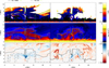 |
Fig. 1. Vertical cuts through the rMHD snapshot intersecting the EB location at x = 11.3 Mm, y = 10.7 Mm. Left column: cut along the y-axis, and right column: cut along the x-axis. We display the temperature, density (on a logarithmic scale), and the vertical velocity together with hmax, 10 830 (solid line) and hmax, D3 (dash-dotted line) as defined in Eq. (2). The red and black boxes in the right panels indicate the region that we zoom into in Figs. 10, 11, and 13. |
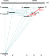 |
Fig. 2. Schematic view of the model atom for He I. The blue lines represent the transitions present in the model atom file, both collisional and radiative. The red lines indicate the He I 10 830 Å and He I D3 spectral lines. Energy levels 1s 2p 3P0, 1, 2 and 3d 3D1, 2, 3 are each depicted in the diagram as one energy level, but they consist of three levels each. The total number of levels in the model atom is 16, 12 of which belong to He I. |
2.2. Multi3D and the model atom
To synthesize the He I D3 and He I 10 830 Å spectral lines, we used the 3D non-LTE radiative transfer code Multi3D (Leenaarts & Carlsson 2009). The code solves the statistical equilibrium equations using multilevel accelerated Λ-iteration (MALI, Rybicki & Hummer 1991, 1992). We used an A4 angle quadrature set consisting of 24 angles. All background opacities including hydrogen were calculated with the Uppsala opacity package (Gustafsson 1973). We used only every second grid point in the x and y direction from the rMHD snapshot for our radiative transfer calculations and the top boundary was clipped, so that the input cube was reduced to dimensions 384 × 384 × 606.
The helium model atom is a simplified 16-level version of the 33-level model atom used by Golding et al. (2014), where the sources of the atomic data are listed in detail. It contains 12 He I levels, 3 He II levels, and the He III continuum. In Fig. 2.2 we show the details of the included energy levels and transitions in He I. Our primary goal is to study the He I D3 and He I 10 830 Å spectral lines that are part of the triplet system. To do this, we included all seven levels that make up these transitions unaltered: 1s 2s 3S1, 1s 2p 3P0, 1, 2, and 1s 3d 3D1, 2, 3, while the 1s 3s 3S2 level and the 1s 3p 3P0, 1, 2 levels were merged. In the singlet system, we included the ground-level 1s21S0 and levels 1s 2s 1S0 and 1s 2p 1P1. Levels 1s 3s 1S0 and 1s 3p 1P1 were merged. No higher excited states of neutral helium were used. In the He II atom, only the He II continuum level was kept unchanged. Levels 2p 2P and 2s 2S
 were merged, as were levels 3s 2S
 , 3p 2P
 , and 3d 2D
 .
.
We also added collisional transitions to the model atom that were missing in the original 33-level model atom. The most important missing collisional transitions were those between the energetically close J-split sublevels of the He I 10 830 Å and He I D3 levels themselves (e.g., 3P0 to 3P1) because these collisional rates are roughly ten orders of magnitude higher than the collisional rates between 3P0 and 3D1, for example. The rates were obtained with the Van Regemorter prescription for collisional excitation (van Regemorter 1962).
The helium model atom includes 26 bound-bound transitions, 62 collisional transitions, and 15 bound-free transitions. The frequency grid contains 1139 points, among which the He I 10 830 Å and He I D3 transitions are sampled with 278 frequency points each. Of these 278 frequency points, 226 sample the lines equidistantly between −224 and +224 km s−1. This reaches the highest chromospheric velocities in the rMHD snapshot.
Coronal radiation is included in the Multi3D calculations as described in detail by Leenaarts et al. (2016). The coronal emissivity is defined as
with ne the electron number density, nH the hydrogen number density and Λν(T) the coronal emissivity per electron and per hydrogen atom as a function of temperature. Λν(T) is calculated from CHIANTI (Dere et al. 2009) with the assumption of coronal equilibrium ionization for all elements with lines present in the EUV spectrum shortward of the ionization edge of He I at 504 Å. These calculations do not include hydrogen and helium lines because these are already accounted for in Multi3D as background source and active element, respectively. The coronal emissivity ψν calculated with CHIANTI is then remapped onto the coarse frequency grid used by Multi3D while preserving the frequency-integrated emissivity.
2.3. Observational data
The He I 10 830 Å and He I D3 spectra were obtained from raster scans with SST/TRIPPEL on 2015 August 1 between 07:51 UT and 10:10 UT. The data acquisition and reduction is described in detail in Libbrecht et al. (2017).
3. Results
3.1. Helium spectra within the snapshot domain
Before we focus on the EB, we briefly consider the entire snapshot domain. Vertical cuts of the rMHD snapshot are shown in Fig. 1, where the EB is present in both columns at x = 11, y = 11 Mm. In the EB location, the temperature rises steeply to coronal values of about 105 − 106 K, the density drops, and bidirectional jets are present with velocities of about 100 km s−1.
In Fig. 1 we display hmax, ℓ of He I 10 830 Å and He I D3, which is defined as
![$$ \begin{aligned} h_{\max ,\ell }=\max \left[h_{\nu _{\ell }}(\tau _{\nu _{\ell }}=1)\right], \end{aligned} $$](/articles/aa/full_html/2021/08/aa39788-20/aa39788-20-eq7.gif)
where ℓ corresponds to the transition and νℓ to all frequencies that sample the corresponding transition. With optically thick line formation, the quantity hmax, ℓ corresponds to the height at which the line core of the transition is formed. In the snapshot displayed in Figs. 1 and 3, hmax, 10 830 is situated everywhere at the interface between the chromosphere and the transition region, where the temperature rises steeply to coronal temperatures. The line formation of He I 10 830 Å is optically thick throughout the snapshot. The He I D3 line is generally formed at lower heights than He I 10 830 Å because its opacity is lower. The He I D3 absorption fluctuates between being optically thick and optically thin. The optically thin state is obvious in locations in which hmax, D3 suddenly drops to the photosphere. The vertical cuts in Fig. 1 demonstrate that flux emergence in the simulation has pushed the corona upward in a large part of the domain toward heights of 6−8 Mm. Regions in which the transition region is situated at a height of around 2 Mm are x = 0 − 4 Mm and x = 18 − 24 Mm, for instance. In these regions, the formation heights of He I D3 and He I 10 830 Å coincide.
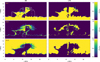 |
Fig. 3. Vertical cuts through the rMHD snapshot intersecting the y-axis at the EB location y = 10.7 Mm. Left column: statistical equilibrium (SE) He I, II, and III population relative to the total population. Right column: LTE He I, II, and III populations relative to the total population. hmax, 10 830 (solid line) and hmax, D3 (dash-dotted line) are plotted in the upper left panel; see the definition in Eq. (2). The white boxes in the left panels indicate the region that we zoom into in Figs. 10, 11, and 13. |
Even though Bifrost treats ionization in LTE in this simulation, with its implications for the heat budget, Multi3D takes non-LTE ionization of helium with the assumption of statistical equilibrium (SE) into account. The difference between SE and LTE helium ionization is shown in Fig. 3. The SE case takes radiation into account, which causes ionization to become nonlocal. Therefore the He II region is more diffuse than in the LTE case, where it simply follows the steep temperature stratification. The opacity in the He I triplet system scales with the He II population because the triplet system is generally populated through recombination cascades from the He II continuum (PRM). Sufficient He I has to be available at the same time as He II in order to populate the He I triplet levels. The vertical cuts demonstrate that it is more likely in the SE case that substantial He II and He I coexist at the same locations. It is therefore important to take SE helium ionization into account to obtain more realistic He I 10 830 Å and He I D3 intensities. Golding et al. (2014) used time-dependent modeling in 1D to show that even the assumption of SE is not valid under dynamic conditions, and full time-dependent modeling is required to obtain the correct helium intensities. This is not yet feasible in 3D, however.
The emergent line core intensities of He I 10 830 Å and He I D3 are shown in Fig. 4. We compare them with observations of a flux emergence region in He I 10 830 Å and He I D3 (same observations as in Libbrecht et al. 2017).
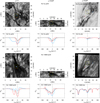 |
Fig. 4. Comparison of a simulated and observed flux emergence region in He I 10 830 Å and He I D3. Top two rows: He I D3 images and spectra, and lower two rows: He I 10 830 Å images and spectra. Left column: synthetic data at μ = 1, middle column: synthetic data at μ = 0.27, and right column: observed data at μ = 0.27. The He I D3 observed image is normalized by the local continuum. The red and blue squares in the images indicate areas over which the spectra are averaged that are displayed in the corresponding color in the panel below the image. The black spectrum is an average over the entire field of view shown in the image. The He I 10 830 Å observed spectral region also contains a Si I line at vLOS ∼ −85 km s−1 and two telluric lines at vLOS ∼ 50 km s−1 and vLOS ∼ 100 km s−1. The vertical black lines on the spectra indicate the wavelength position at which the image is shown. We have adopted the observer point of view for Doppler shifts in which a negative vLOS corresponds to a blueshift in the spectral line. The larger yellow squares correspond to the regions that are zoomed into in Fig. 5. Vertical slices along the white markers in the synthetic μ = 1 images are shown in Figs. 1 and 3. |
The synthetic and observed He I 10 830 Å image show long and thick fibrils and a thick canopy structure, while the less active areas appear to be more grainy. The average synthetic He I 10 830 Å absorption equals 0.6 ILC, where ILC is the local continuum intensity at μ = 0.27. This value is similar to the observed average absorption at the same μ-angle.
For the He I D3 line the difference is more substantial: The observations have to be normalized by the local measured continuum intensity to even notice the He I D3 absorption, while the synthetic absorption becomes optically thick in many locations and is very obvious over almost the entire domain. The absorption in the average synthetic He I D3 profile reaches 0.7 ILC, and the average observed absorption is 0.9 ILC for μ = 0.27.
The rMHD snapshot harbors velocities of about 100 km s−1 at the He I 10 830 Å and He I D3 formation height, while velocities this high are very rare in He I D3 and He I 10 830 Å observations of flux emergence regions. These extreme velocities cause the synthetic line profiles to exhibit multiple velocity components and hence a more complicated appearance than the observed profiles.
3.2. EB helium profiles
Figure 5 shows a zoom on an EB in the synthetic and observed data and the He I D3 and He I 10 830 Å spectra. First, we concentrate on the synthetic images and spectra at μ = 1. The EB has a slightly elongated appearance and is bright in the line core images of He I D3 and He I 10 830 Å. The EB has a He I 10 830 Å line profile in pure emission, while most He I D3 profiles are pure absorption profiles. However, some of the synthetic He I D3 profiles show a combination of emission and absorption, with the emission redshifted with velocities of ∼70 km s−1.
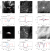 |
Fig. 5. Comparison of a simulated and an observed EB in He I 10 830 Å and He I D3. Top two rows: He I D3 images and spectra, and lower two rows: He I 10 830 Å images and spectra. Left column: synthetic data at μ = 1, middle column: synthetic data at μ = 0.27, and right column: observed data at μ = 0.27. The He I D3 observed image is normalized by the local continuum. The red and blue squares in the images indicate the position of the spectra that are displayed in the corresponding color in the panel below the image. The white square corresponds to the black profile. The He I 10 830 Å observed spectral region also contains a Si I line at vLOS ∼ −85 km s−1 and two telluric lines at vLOS ∼ 50 km s−1 and vLOS ∼ 100 km s−1. The vertical black lines on the spectra indicate the wavelength position at which the image is shown. We have adopted the observer point of view for Doppler shifts in which a negative vLOS corresponds to a blueshift in the spectral line. The label Lem indicates the pixel with maximum emission in He I D3, which we study in detail in Sect. 3.3. The black spectrum is an average over the entire field of view shown in the image. The emission feature in the observed He I D3 spectrum at vLOS ∼ 40 km s−1 is an artifact resulting from a telluric correction applied to the spectra. Details of this procedure can be found in Libbrecht et al. (2017). |
The appearance of the EB changes drastically when the outgoing intensity is calculated along highly inclined rays. At an angle of μ = 0.27, the EB is one-pixel thin and very elongated in He I 10 830 Å and He I D3, with a length of more than one arcsec. At this viewing angle, all synthetic He I D3 and He I 10 830 Å EB profiles are a combination of emission in the line wing and absorption in the line core. This demonstrates that the combination of obstruction by fibrils and the line-of-sight velocity are the dominant properties that shape the helium EB profiles.
The synthetic He I D3 and He I 10 830 Å EB profiles at μ = 0.27 match the observed profiles on a qualitative level: occurrence of emission in the wing, absorption in the core, and the dynamics appear to be largely reproduced. Strong blue- and/or redshifts are present, depending on the viewing angle. Moreover, the broadening is on the same order of magnitude in the observed and the synthetic profiles. However, the synthetic emission features are much stronger than the observed ones: The maximum observed He I D3 emission is only at ∼1.1 ILC, while the synthetic He I D3 emission is at ∼3.5 ILC when they are compared at equal viewing angles of μ = 0.27.
Despite the differences between the observed and synthetic profiles, the 3D rMHD simulation provides a remarkable opportunity to study line formation in detail. This cannot be done with the observations. It is encouraging that emission is present in the synthetic EB profiles and that there is some qualitative overlap between the observations and simulation, and we aim to determine the cause of the synthetic emission. To do this, we selected the profile with maximum He I D3 emission for a more detailed study. We call the location at which this profile is located Lem.
3.3. EB helium line formation
In order to study line formation, we consider the μ = 1 case. Figures 6 and 7 show diagrams that break down the different factors that make up the contribution function Cν to the He I D3 and He I 10 830 Å line profiles (Carlsson & Stein 1997),
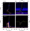 |
Fig. 6. Line formation plot with all factors that make up the contribution function (Eq. (3)) of the EB He I D3 emission profile at location Lem (see Fig. 5) and at a heliocentric viewing angle of μ = 1. Top left: opacity χν divided by optical depth τν. The hmax, ℓ surface (Eq. (2)) is shown as a solid red line and the vertical velocity vz as a solid white line. Top right: total source function |

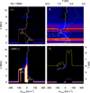 |
Fig. 7. Same as Fig. 6, but for He I 10 830 Å Line formation plot with all factors that make up the contribution function (Eq. (3)) of the EB He I 10 830 Å emission profile at location Lem (see Fig. 5) and at a heliocentric viewing angle of μ = 1. |
with χν the opacity and τν the optical depth. The source function  equals the total source function, which combines the line source function
  and the continuum source function
  as
as
where  and jν is the emissivity. The terms can be separated by calculating the line source function Sl through
where the subscript l stands for lower level and u for upper level of the transition. n is the population of the level, A is the Einstein coefficient for spontaneous deexcitation, and B is the Einstein coefficient for stimulated (de-)excitation.
The contribution function demonstrates that the absorption in the He I D3 profile is formed in a thin slab at a height of ∼4 Mm, while the emission is formed in a thin layer at ∼0.8 Mm, much deeper in the atmosphere. The same is true for He I 10 830 Å, but the component formed at ∼4 Mm is mostly in emission as well. The line-of-sight velocity has the opposite sign at 0.8 compared to 4 Mm so that the absorption component becomes blueshifted and the emission component becomes redshifted. The τν = 1 surfaces of both lines demonstrate that the height of the main opacity sources highly depends on frequency because it shoots straight up from the photosphere into the upper chromosphere and back without a smooth transition. This is also what we expect to see when we scan through images at different frequencies of the He I D3 and He I 10 830 Å lines. We expect the value of the total source function  compared to the continuum source function
  to indicate whether absorption or emission is expected for a certain contribution at a certain height. Therefore we provide a line plot of the source function of He I D3 at different frequencies with height in Fig. 8. The emission is present because the source function at 0.8 Mm is higher than the source function at 0 Mm, where the continuum is formed. To understand the real cause of the emission and absorption, we investigated why the source function and opacity behave as they do.
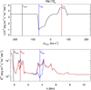 |
Fig. 8. Comparison of the emergent intensity and the source function of an EB He I D3 emission profile. Top panel: emergent intensity. Three vertical lines in black, blue, and red correspond to three selected frequencies νcont, νabs, and νem. Bottom panel: total source function at three different frequencies |


First of all, we have to understand how the triplet levels are populated. Figure 9 shows a schematic rate diagram where we plot the total net rates N, defined as


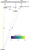 |
Fig. 9. Net rate N at location Lem (see Fig. 4) and height of maximum emissivity in He I D3. The model atom incorporates 12 levels in neutral helium (16 in total). We have combined many of these levels to increase the readability of the diagram, but they are treated separately in the calculations (see Sect. 2 and Fig. 2.2). |
R are the radiative rates, and C are the collisional rates between levels l and u or u and l. We define Nr and Nc as the total radiative net rate and the total collisional net rate, respectively. We combined many of the levels and net rates accordingly for a clear visualization. If Nr > Nc, the arrow in Fig. 9 is plotted as a full line, and if Nc > Nr, the arrow is plotted as a dotted line. However, the color of the line still represents the total net rate N, taking into account both radiative and collisional transitions.
From Fig. 9 we deduce that the triplet levels are populated by photoionization-recombination. The total number of transitions from the He I ground level to the He II continuum equals N = 8 × 1013 cm−3 s−1, with N ∼ Nr and Nc = −8 × 108 cm−3 s−1 (note the opposite sign). This means that there are a factor 105 more photoionizations than collisional recombinations.
Recombination from He II into the excited triplet system of neutral helium is also radiatively dominated, while the net collisional rates are a factor ten lower and in the opposite direction. Radiative ionizations from the ground level of the triplet state (indicated as 2s in Fig. 9) balance the populations in the triplet system. No collisions populate the triplet system from the ground level of He I directly, instead, a relatively strong downward collisional rate is obtained. All these properties prove that photoionization-recombination is the dominant populating mechanism for the triplet system of He I at this location.
Next, we investigated the source of those photoionizing photons at the EB location. To do this, we studied a close-up of a vertical cutout along the x-axis corresponding to the boxes indicated in Figs. 1 and 3. The cutout is shown in Fig. 10 at a height of 0.3−2 Mm. This is the region in which He I D3 emission is formed: hem = 0.8 Mm in Fig. 8. Figure 10 shows that the very hot part of the bomb with a temperature of T > 106 K is located at heights ranging between 0.8 and 1.5 Mm, in which all helium is doubly ionized, so that only He III is present. The mass and electron density are ∼3 orders of magnitude lower in the high-temperature region of the EB than outside the EB. Outside the EB, mass and electron density are quite high and quickly increase with depth because the location is deep in the atmosphere, only 0.8 Mm above the τ500 = 1 surface.
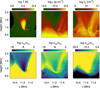 |
Fig. 10. Properties of a cutout along the x-axis of the lower part of the EB (indicated as a white box in Figs. 1 and 3). Top row: temperature T, mass density ρ, and electron number density ne are shown on a log scale. Bottom row: ratio of the number density of He I, He II, and He III to the total number density of helium ntot are shown on a log scale. The black and white markers show the position of the He I D3 profile shown in Figs. 6 and 8 at locations Lem (see Fig. 5) and hem (see Fig. 8). |
Figure 10 indicates that a narrow shell is present around the EB in which He II is present. This shell is vitally important to the formation of the He I D3 and He I 10 830 Å lines. We know that photoionization-recombination is the mechanism that populates the triplet system of He I. In Fig. 11 we therefore display the EUV radiation field consisting of ionizing radiation integrated between ν = 0 and  , with λion = 504 Å being the ionization edge of He II,
 |
Fig. 11. Properties of a cutout along the x-axis of the lower part of the EB (indicated as a white box in Figs. 1 and 3). Top left to right: frequency-integrated ionizing radiation field Jion (see Eq. (9)), where jion, abs is absorbed (see Eq. (14)), and total number of recombinations in the triplet system Nrec as defined Eq. (15). Bottom: composite panel of Jion, jion, abs, and Nrec. The black markers indicate the position of the He I D3 profile shown in Figs. 6 and 8 at locations Lem (see Fig. 5) and hem (see Fig. 8). The black contours show the regions in which |

with Jν defined as the mean intensity  . The emissivity jion of this mean intensity can be written as the sum of the background emissivity
  and the emissivity originating from EUV helium lines themselves,
  ,
,
The background emissivity  consists of all other coronal and transition region EUV line emissivities, except for those of helium EUV lines.
  can be written as the sum of two contributions: thermal photons and scattered photons (see also Eq. (17)),
where ϵb is the destruction probability of background photons,  is defined as the thermal contribution to the background emissivity, and
  is the scattering contribution. The quantity Jion shown in Fig. 11 indicates where the ionizing radiation is present, while the contours in Fig. 11 show where the photons are thermally created because the contours map the regions in which

The ionizing background photons are thermally created close to the lower boundary of the EB. Subsequently, these ionizing photons can propagate only within the hot part of the EB and are absorbed in a shell around the EB, as depicted by the quantity jion, abs in Fig. 11, defined as
The recombination rate into the triplet system is calculated as
and is proportional to the population of the He II continuum nc, which peaks in a thin shell around the EB and around the shell in which jion, abs peaks.
Because the location in which  peaks is known exactly, we can derive the temperature and electron density required to emit this radiation and hence populate the levels. We selected pixels where
  erg s−1 cm−3 ster−1 to display in Fig. 12. The value of
  peaks in regions that have a temperature between 2 × 10⁴ and 2 × 10⁶ K and an electron density between 1011 and 1013 cm−3. Data points with the highest
  can have very different temperatures, but all have high electron densities of 1013 cm−3.
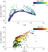 |
Fig. 12. Top: all pixels in Fig. 11 in which |


When the triplet levels are populated, we still need to study how the lines are formed exactly and why the emission is present. In order to determine whether thermal processes play a role, it is useful to look at the photon destruction probability with a two-level atom approximation,
where B(T) equals the Planck function. In the two-level atom approximation, the source function then consists of a thermal and a scattering part, quantified by ϵ,
with B(T) the Planck function, and  equals
where ϕ(ν − ν0) is the line profile and ν0 the line core frequency. The photon destruction probability ϵ is shown in Fig. 13 and is a measure for collisional coupling to the local conditions in the plasma. In other words, it shows how close the conditions are to LTE. It roughly follows the variation of the electron density. The value for ϵ equals 10−2 for He I D3 and 10−1 for He I 10 830 Å at Lem (see Fig. 5) and hem (see Fig. 8). These values are relatively high for chromospheric lines: We can compare them with Figs. 12–15 of Bjørgen et al. (2019), who showed that most chromospheric diagnostics only reach these values in flare ribbons.
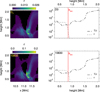 |
Fig. 13. Properties of a cutout along the x-axis of the lower part of the EB (indicated as a white box in Figs. 1 and 3). Top left: destruction probability ϵ of He I D3. Bottom left: same for He I 10 830 Å. Top right: thermalization length 1/ϵ (see Eq. (16)) in units of optical depth as a function of height at location Lem (see Fig. 5), plotted together with the optical depth τν at νem (see Fig. 8). hem as defined in Fig. 8 is overplotted as a vertical line. Bottom right: same for He I 10 830 Å. |
It is useful to compare the thermalization length 1/ϵ in units of optical depth with the optical depth τν, which is shown in the right panels of Fig. 13. The photons are thermalized when τν ≥ 1/ϵ. We read from Fig. 13 that the opacity of the shell around the EB is optically thick in He I D3 and He I 10 830 Å. The photons subsequently escape at hem when τν drops below one. The temperature in this optically thick layer is in the range 7 × 10³ − 104 K. This is higher than the temperature at which the continuum radiation is formed, and therefore emission is produced due to thermalization. The photons subsequently escape outside the optically thick thermalized part of the layer where τν drops below one.
Another possible mechanism that could generate emission are recombination cascades in the triplet system. These are difficult to quantify, however, because the two-level approximation is no longer valid, and Eq. (17) should be rewritten in the following way (see Rutten & Uitenbroek 2012):

Here, ϵ′ is the photon destruction probability, but it cannot be easily determined, and Eq. (16) does not apply in this case. δ is the fraction of photons that are created by alternative processes (for example, recombination cascades) and B(T′) is the Planck function calculated using a virtual temperature T′ that corresponds to the radiation temperature of the photons created by recombination cascades. For He I 10 830 Å, we are quite certain that recombination cascades are negligible: The line source function coincides with the temperatures in the thermalized shell because the value of ϵ is higher. This strongly suggests that thermal processes dominate. For He I D3, ϵ is one order of magnitude smaller and the temperature and source function are only partially coupled. This means that electron cascades might contribute to the formation of emission in He I D3, but tehy likely do not dominate.
4. Discussion
The first question we address is whether the rMHD simulation presented in Hansteen et al. (2019) provides us with a realistic model of an EB. On the positive side, the physics that are associated with reconnection in EBs are present: colliding vertical magnetic fields, and resulting bidirectional jets. The main spectral characteristics of EBs/UV bursts are also reproduced in Hα, Si IV 1400 Å, and Ca II 8542 Å. The least realistic part of the simulation in the context of our calculations is that coronal radiative losses were treated in 1D. A strongly heated column is therefore present immediately above the EB starting at a height of ∼4 Mm and extends upward throughout the domain. If coronal losses were treated in 3D, they would have propagated in all directions, which would likely have a tempering effect. However, we focused on the emission in He I D3 generated in the deep atmosphere at ≤1 Mm. Therefore the emission is not affected by the heated column located above the EB. The He I D3 and He I 10 830 Å profiles that are shown in the middle column of Fig. 5 at a heliocentric angle of μ = 0.27 are not affected by the heated column because the line of sight does not cross this region of the domain.
The largest difference between the observed and synthetic profiles is that the emission peaks are much more intense in the synthetic profiles. It is likely that spatial smearing of the observations by the point spread function of TRIPPEL contributes to this difference. Another important cause of the more intense emission peaks in the simulation is the massive amount of material at chromospheric temperatures in this snapshot. In more quiet-Sun-like environments, the chromosphere is a rather thin layer usually situated between heights of ∼0.5 and 2 Mm. In this case, the violent flux emergence has pushed the chromosphere and transition region up to heights of up to 8 Mm, as displayed in Fig. 1. Realistic or not, this property of the synthetic atmosphere does not affect the physical mechanisms that we propose in this paper, populating the helium triplet levels and generating emission in He I D3 and He I 10 830 Å.
Another question we address is whether it is realistic that the EB/UV burst in the rMHD snapshot reaches temperatures of 106 K. Part of our motivation for this paper originates from discussions and uncertainties about the temperature of EBs, but no estimate in the literature has been higher than 105 K so far. However, these temperatures have always been estimated using chromospheric and transition region spectral lines such as Hα and Si IV 1400 Å. None of these lines would sample plasma with coronal temperatures because these species become fully ionized. Coronal emission from the EB, on the other hand, would be completely absorbed by the overlying cooler plasma. This means that we are observationally blind to this type of temperatures in the deep atmosphere and that we have no straightforward way of determining whether it is possible to reach coronal temperatures in EBs.
Our results show that the ionizing radiation is thermally created at temperatures in the range of 2 × 10⁴ − 106 K and densities between 1011 and 1013 cm−1. This means that at least in our simulation, we require a high temperature in order to generate opacity in He I D3 and He I 10 830 Å through the ionization-recombination mechanism. This ionizing radiation is created locally in the EB and ionizes a cooler layer or shell around it. This is reminiscent of Leenaarts et al. (2016), who showed that a substation part of the He I 10 830 Å opacity is created locally adjacent to hot transition region patches. Similarly, Labrosse & Gouttebroze (2004) modeled a transition region between a cool prominence and a hot surrounding corona and concluded that such an interface layer plays a significant role in the formation of the helium triplet line.
When the triplet levels in neutral helium are populated, the He I 10 830 Å and He I D3 emission is created by thermalization in an optically thick layer around the EB with temperatures between 7 × 10³ and 104 K and electron densities of about 1013 cm−3. There might be a possible but not dominant contribution from recombination cascades to the He I D3 emission.
It is clear that EBs and UV bursts are complex multithermal objects. We can think of them as an onion with a hot core and shells around it in which ionizing radiation is created and absorbed, and recombinations into the triplet system take place. Libbrecht et al. (2017) reported a temperature estimate of EBs in the range of 2 × 10⁴ − 105 K. However, we estimated the lower limit of 2 × 10⁴ K based on the assumption of LTE, not based on the idea of generating local ionizing EUV radiation. In any case, similarly as in Libbrecht et al. (2017), we claim that the presence of He I D3 and He I 10 830 Å emission is an indicator of high temperatures in EBs. This is compatible with the radiative transfer calculations presented by Hansteen et al. (2019), which confirm that even an EB/UV burst of 106 K can be compatible with the observed Hα and Si IV 1400 Å profiles in these objects.
5. Summary and conclusion
We have focused on helium line formation in an EB. We used a synthetic atmosphere generated by an rMHD simulation and used the atmosphere to calculate helium line intensities using the 3D non-LTE code Multi3D, under the assumption of statistical equilibrium.
The EB line profiles of He I 10 830 Å and He I D3 in the simulation show similar properties as the observed line profiles of an EB at equal viewing angle. Emission in the wing is present while the line core is in absorption. The dynamics and the broadening are largely reproduced in the simulation. However, the line intensities of the simulation are different: The emission and the absorption signatures are both stronger in the synthetic profiles than in the observed profiles, at least for the He I D3 line. Moreover, the synthetic emission in He I 10 830 Å is very intense but barely present in the observed profiles.
Encouraged by the qualitative overlap between the synthetic and observed EB He I D3 profiles, we continued the paper to focus on the most intense He I D3 emission profile. The emission part of the He I D3 profile in our simulation is formed low in the atmosphere at a height of ∼1 Mm, and the absorption part is formed much higher at ∼4 Mm, which is reminiscent of the formation of Hα profiles in EBs. We find that photoionization-recombination is the dominant mechanism in populating the helium triplet system inside and outside the EB. The ionizing radiation is thermally created locally inside the EB at temperatures between 2 × 10⁴ and 106 K and electron densities ranging between 1011 and 1013 cm−1, and it is absorbed in a dense and cooler shell around it. Recombinations populate the triplet levels. Emission in He I D3 and He I 10 830 Å is created in a thermalized shell that is optically thick in He I D3 and He I 10 830 Å and has temperatures in the range of 7 × 10³ − 104 K and electron densities between 1012 and 1013 cm−3.
These results suggest that the observation of He I D3 and He I 10 830 Å signatures in EBs/UV bursts indicate temperatures higher than 2 × 10⁴ K. In our case, they are as high as ∼106 K.
Acknowledgments
TL is supported by the Swedish Research Council (2015-03994) and the Swedish National Space Board (128/15). JdlCR is supported by grants from the Swedish Research Council (2015-03994), the Swedish National Space Board (128/15) and the Swedish Civil Contingencies Agency (MSB). This project has received funding from the European Research Council (ERC) under the European Union’s Horizon 2020 research and innovation programme (SUNMAG, grant agreement 759548). JJ is supported by the Research Council of Norway, project 250810, and through its Centres of Excellence scheme, project number 262622. The Institute for Solar Physics is supported by a grant for research infrastructures of national importance from the Swedish Research Council (registration number 2017-00625). The Swedish 1-m Solar Telescope is operated on the island of La Palma by the Institute for Solar Physics of Stockholm University in the Spanish Observatorio del Roque de los Muchachos of the Instituto de Astrofísica de Canarias. The 3D non-LTE radiative transfer calculations were performed on resources provided by the Swedish National Infrastructure for Computing (SNIC) at the High Performance Computing Center North at Umeå University. This research has made use of NASA’s Astrophysics Data System Bibliographic Services.
References
- Andretta, V., & Jones, H. P. 1997, ApJ, 489, 375 [Google Scholar]
- Bello González, N., Danilovic, S., & Kneer, F. 2013, A&A, 557, A102 [NASA ADS] [CrossRef] [EDP Sciences] [Google Scholar]
- Berlicki, A., & Heinzel, P. 2014, A&A, 567, A110 [Google Scholar]
- Bjørgen, J. P., Leenaarts, J., Rempel, M., et al. 2019, A&A, 631, A33 [NASA ADS] [CrossRef] [EDP Sciences] [Google Scholar]
- Carlsson, M., & Leenaarts, J. 2012, A&A, 539, A39 [Google Scholar]
- Carlsson, M., & Stein, R. F. 1997, ApJ, 481, 500 [Google Scholar]
- Carlsson, M., Hansteen, V. H., Gudiksen, B. V., Leenaarts, J., & De Pontieu, B. 2016, A&A, 585, A4 [Google Scholar]
- Centeno, R., Trujillo Bueno, J., Uitenbroek, H., & Collados, M. 2008, ApJ, 677, 742 [Google Scholar]
- Chen, Y., Tian, H., Peter, H., et al. 2019, ApJ, 875, L30 [NASA ADS] [CrossRef] [Google Scholar]
- Danilovic, S. 2017, A&A, 601, A122 [Google Scholar]
- Danilovic, S., Solanki, S. K., Barthol, P., et al. 2017, ApJS, 229, 5 [Google Scholar]
- De Pontieu, B., Title, A. M., Lemen, J. R., et al. 2014, Sol. Phys., 289, 2733 [NASA ADS] [CrossRef] [Google Scholar]
- Dere, K. P., Landi, E., Young, P. R., et al. 2009, A&A, 498, 915 [Google Scholar]
- Ding, M. D., Li, H., & Fang, C. 2005, A&A, 432, 699 [Google Scholar]
- Ellerman, F. 1917, ApJ, 46, 298 [NASA ADS] [CrossRef] [Google Scholar]
- Fang, C., Hao, Q., Ding, M.-D., & Li, Z. 2017, Res. Astron. Astrophys., 17, 031 [NASA ADS] [CrossRef] [Google Scholar]
- Goldberg, L. 1939, ApJ, 89, 673 [Google Scholar]
- Golding, T. P., Carlsson, M., & Leenaarts, J. 2014, ApJ, 784, 30 [Google Scholar]
- Gudiksen, B. V., Carlsson, M., Hansteen, V. H., et al. 2011, A&A, 531, A154 [Google Scholar]
- Gustafsson, B. 1973, Upps. Astron. Obs. Ann., 5, 6 [Google Scholar]
- Hansteen, V. H., Archontis, V., Pereira, T. M. D., et al. 2017, ApJ, 839, 22 [NASA ADS] [CrossRef] [Google Scholar]
- Hansteen, V., Ortiz, A., Archontis, V., et al. 2019, A&A, 626, A33 [Google Scholar]
- Judge, P. G., Kleint, L., & Sainz Dalda, A. 2015, ApJ, 814, 100 [Google Scholar]
- Kiselman, D., Pereira, T. M. D., Gustafsson, B., et al. 2011, A&A, 535, A14 [Google Scholar]
- Labrosse, N., & Gouttebroze, P. 2004, ApJ, 617, 614 [Google Scholar]
- Lagg, A., Woch, J., Solanki, S. K., & Krupp, N. 2007, A&A, 462, 1147 [NASA ADS] [CrossRef] [EDP Sciences] [Google Scholar]
- Laming, J. M., & Feldman, U. 1992, ApJ, 386, 364 [Google Scholar]
- Leenaarts, J., & Carlsson, M. 2009, in The Second Hinode Science Meeting: Beyond Discovery-Toward Understanding, eds. B. Lites, M. Cheung, T. Magara, J. Mariska, & K. Reeves, ASP Conf. Ser., 415, 87 [NASA ADS] [Google Scholar]
- Leenaarts, J., Golding, T., Carlsson, M., Libbrecht, T., & Joshi, J. 2016, A&A, 594, A104 [Google Scholar]
- Libbrecht, T., Joshi, J., Rodríguez, J. D. L. C., Leenaarts, J., & Ramos, A. A. 2017, A&A, 598, A33 [Google Scholar]
- Libbrecht, T., de la Cruz Rodríguez, J., Danilovic, S., Leenaarts, J., & Pazira, H. 2019, A&A, 621, A35 [Google Scholar]
- Liu, C., Xu, Y., Deng, N., et al. 2013, ApJ, 774, 60 [Google Scholar]
- Nelson, C. J., Shelyag, S., Mathioudakis, M., et al. 2013, ApJ, 779, 125 [Google Scholar]
- Ortiz, A., Hansteen, V. H., Nóbrega-Siverio, D., & van der Voort, L. R. 2020, A&A, 633, A58 [Google Scholar]
- Peter, H., Tian, H., Curdt, W., et al. 2014, Science, 346, 1255726 [Google Scholar]
- Rutten, R. J., & Uitenbroek, H. 2012, A&A, 540, A86 [Google Scholar]
- Rybicki, G. B., & Hummer, D. G. 1991, A&A, 245, 171 [NASA ADS] [Google Scholar]
- Rybicki, G. B., & Hummer, D. G. 1992, A&A, 262, 209 [NASA ADS] [Google Scholar]
- Scharmer, G. B., Bjelksjo, K., Korhonen, T. K., Lindberg, B., & Petterson, B. 2003, in Innovative Telescopes and Instrumentation for Solar Astrophysics, eds. S. L. Keil, & S. V. Avakyan, SPIE Conf. Ser., 4853, 341 [Google Scholar]
- Tian, H., Xu, Z., He, J., & Madsen, C. 2016, ApJ, 824, 96 [CrossRef] [Google Scholar]
- van Regemorter, H. 1962, ApJ, 136, 906 [Google Scholar]
- Vissers, G. J. M., van der Rouppe Voort, L. H. M., Rutten, R. J., Carlsson, M., & De Pontieu, B. 2015, ApJ, 812, 11 [Google Scholar]
- Vissers, G. J. M., de la Cruz Rodríguez, J., Libbrecht, T., et al. 2019, A&A, 627, A101 [Google Scholar]
- Xu, Y., Cao, W., Ding, M., et al. 2016, ApJ, 819, 89 [Google Scholar]
- Zeng, Z., Qiu, J., Cao, W., & Judge, P. G. 2014, ApJ, 793, 87 [Google Scholar]
- Zirin, H. 1975, ApJ, 199, L63 [Google Scholar]
All Figures
|
Fig. 1. Vertical cuts through the rMHD snapshot intersecting the EB location at x = 11.3 Mm, y = 10.7 Mm. Left column: cut along the y-axis, and right column: cut along the x-axis. We display the temperature, density (on a logarithmic scale), and the vertical velocity together with hmax, 10 830 (solid line) and hmax, D3 (dash-dotted line) as defined in Eq. (2). The red and black boxes in the right panels indicate the region that we zoom into in Figs. 10, 11, and 13. |
| In the text | |
|
Fig. 2. Schematic view of the model atom for He I. The blue lines represent the transitions present in the model atom file, both collisional and radiative. The red lines indicate the He I 10 830 Å and He I D3 spectral lines. Energy levels 1s 2p 3P0, 1, 2 and 3d 3D1, 2, 3 are each depicted in the diagram as one energy level, but they consist of three levels each. The total number of levels in the model atom is 16, 12 of which belong to He I. |
| In the text | |
|
Fig. 3. Vertical cuts through the rMHD snapshot intersecting the y-axis at the EB location y = 10.7 Mm. Left column: statistical equilibrium (SE) He I, II, and III population relative to the total population. Right column: LTE He I, II, and III populations relative to the total population. hmax, 10 830 (solid line) and hmax, D3 (dash-dotted line) are plotted in the upper left panel; see the definition in Eq. (2). The white boxes in the left panels indicate the region that we zoom into in Figs. 10, 11, and 13. |
| In the text | |
|
Fig. 4. Comparison of a simulated and observed flux emergence region in He I 10 830 Å and He I D3. Top two rows: He I D3 images and spectra, and lower two rows: He I 10 830 Å images and spectra. Left column: synthetic data at μ = 1, middle column: synthetic data at μ = 0.27, and right column: observed data at μ = 0.27. The He I D3 observed image is normalized by the local continuum. The red and blue squares in the images indicate areas over which the spectra are averaged that are displayed in the corresponding color in the panel below the image. The black spectrum is an average over the entire field of view shown in the image. The He I 10 830 Å observed spectral region also contains a Si I line at vLOS ∼ −85 km s−1 and two telluric lines at vLOS ∼ 50 km s−1 and vLOS ∼ 100 km s−1. The vertical black lines on the spectra indicate the wavelength position at which the image is shown. We have adopted the observer point of view for Doppler shifts in which a negative vLOS corresponds to a blueshift in the spectral line. The larger yellow squares correspond to the regions that are zoomed into in Fig. 5. Vertical slices along the white markers in the synthetic μ = 1 images are shown in Figs. 1 and 3. |
| In the text | |
|
Fig. 5. Comparison of a simulated and an observed EB in He I 10 830 Å and He I D3. Top two rows: He I D3 images and spectra, and lower two rows: He I 10 830 Å images and spectra. Left column: synthetic data at μ = 1, middle column: synthetic data at μ = 0.27, and right column: observed data at μ = 0.27. The He I D3 observed image is normalized by the local continuum. The red and blue squares in the images indicate the position of the spectra that are displayed in the corresponding color in the panel below the image. The white square corresponds to the black profile. The He I 10 830 Å observed spectral region also contains a Si I line at vLOS ∼ −85 km s−1 and two telluric lines at vLOS ∼ 50 km s−1 and vLOS ∼ 100 km s−1. The vertical black lines on the spectra indicate the wavelength position at which the image is shown. We have adopted the observer point of view for Doppler shifts in which a negative vLOS corresponds to a blueshift in the spectral line. The label Lem indicates the pixel with maximum emission in He I D3, which we study in detail in Sect. 3.3. The black spectrum is an average over the entire field of view shown in the image. The emission feature in the observed He I D3 spectrum at vLOS ∼ 40 km s−1 is an artifact resulting from a telluric correction applied to the spectra. Details of this procedure can be found in Libbrecht et al. (2017). |
| In the text | |
|
Fig. 6. Line formation plot with all factors that make up the contribution function (Eq. (3)) of the EB He I D3 emission profile at location Lem (see Fig. 5) and at a heliocentric viewing angle of μ = 1. Top left: opacity χν divided by optical depth τν. The hmax, ℓ surface (Eq. (2)) is shown as a solid red line and the vertical velocity vz as a solid white line. Top right: total source function |
| In the text | |
|
Fig. 7. Same as Fig. 6, but for He I 10 830 Å Line formation plot with all factors that make up the contribution function (Eq. (3)) of the EB He I 10 830 Å emission profile at location Lem (see Fig. 5) and at a heliocentric viewing angle of μ = 1. |
| In the text | |
|
Fig. 8. Comparison of the emergent intensity and the source function of an EB He I D3 emission profile. Top panel: emergent intensity. Three vertical lines in black, blue, and red correspond to three selected frequencies νcont, νabs, and νem. Bottom panel: total source function at three different frequencies |
| In the text | |
|
Fig. 9. Net rate N at location Lem (see Fig. 4) and height of maximum emissivity in He I D3. The model atom incorporates 12 levels in neutral helium (16 in total). We have combined many of these levels to increase the readability of the diagram, but they are treated separately in the calculations (see Sect. 2 and Fig. 2.2). |
| In the text | |
|
Fig. 10. Properties of a cutout along the x-axis of the lower part of the EB (indicated as a white box in Figs. 1 and 3). Top row: temperature T, mass density ρ, and electron number density ne are shown on a log scale. Bottom row: ratio of the number density of He I, He II, and He III to the total number density of helium ntot are shown on a log scale. The black and white markers show the position of the He I D3 profile shown in Figs. 6 and 8 at locations Lem (see Fig. 5) and hem (see Fig. 8). |
| In the text | |
|
Fig. 11. Properties of a cutout along the x-axis of the lower part of the EB (indicated as a white box in Figs. 1 and 3). Top left to right: frequency-integrated ionizing radiation field Jion (see Eq. (9)), where jion, abs is absorbed (see Eq. (14)), and total number of recombinations in the triplet system Nrec as defined Eq. (15). Bottom: composite panel of Jion, jion, abs, and Nrec. The black markers indicate the position of the He I D3 profile shown in Figs. 6 and 8 at locations Lem (see Fig. 5) and hem (see Fig. 8). The black contours show the regions in which |
| In the text | |
|
Fig. 12. Top: all pixels in Fig. 11 in which |
| In the text | |
|
Fig. 13. Properties of a cutout along the x-axis of the lower part of the EB (indicated as a white box in Figs. 1 and 3). Top left: destruction probability ϵ of He I D3. Bottom left: same for He I 10 830 Å. Top right: thermalization length 1/ϵ (see Eq. (16)) in units of optical depth as a function of height at location Lem (see Fig. 5), plotted together with the optical depth τν at νem (see Fig. 8). hem as defined in Fig. 8 is overplotted as a vertical line. Bottom right: same for He I 10 830 Å. |
| In the text | |
Current usage metrics show cumulative count of Article Views (full-text article views including HTML views, PDF and ePub downloads, according to the available data) and Abstracts Views on Vision4Press platform.
Data correspond to usage on the plateform after 2015. The current usage metrics is available 48-96 hours after online publication and is updated daily on week days.
Initial download of the metrics may take a while.