| Issue |
A&A
Volume 642, October 2020
|
|
|---|---|---|
| Article Number | A89 | |
| Number of page(s) | 18 | |
| Section | Cosmology (including clusters of galaxies) | |
| DOI | https://doi.org/10.1051/0004-6361/202037965 | |
| Published online | 09 October 2020 | |
X-ray study of the merging galaxy cluster Abell 3411-3412 with XMM-Newton and Suzaku
1
Leiden Observatory, Leiden University, PO Box 9513, 2300 RA Leiden, The Netherlands
e-mail: xyzhang@strw.leidenuniv.nl
2
SRON Netherlands Institute for Space Research, Sorbonnelaan 2, 3584 CA Utrecht, The Netherlands
3
Kavli Institute for the Physics and Mathematics of the Universe (WPI), The University of Tokyo, Kashiwa, Chiba 277-8583, Japan
Received:
15
March
2020
Accepted:
29
July
2020
Context. Previous Chandra observations of the Abell 3411-3412 merging galaxy cluster system revealed an outbound bullet-like sub-cluster in the northern part and many surface brightness edges at the southern periphery, where multiple diffuse sources are also reported from radio observations. Notably, a southeastern radio relic associated with fossil plasma from a radio galaxy and with a detected X-ray edge provides direct evidence of shock re-acceleration. The properties of the reported surface brightness features have yet to be constrained from a thermodynamic viewpoint.
Aims. We use the XMM-Newton and Suzaku observations of Abell 3411-3412 to reveal the thermodynamical nature of the previously reported re-acceleration site and other X-ray surface brightness edges. We also aim to investigate the temperature profile in the low-density outskirts with Suzaku data.
Methods. We performed both imaging and spectral analysis to measure the density jump and the temperature jump across multiple known X-ray surface brightness discontinuities. We present a new method to calibrate the vignetting function and spectral model of the XMM-Newton soft proton background. Archival Chandra, Suzaku, and ROSAT data are used to estimate the cosmic X-ray background and Galactic foreground levels with improved accuracy compared to standard blank sky spectra.
Results. At the southeastern edge, temperature jumps revealed by both XMM-Newton and Suzaku point to a ℳ ∼ 1.2 shock, which agrees with the previous result from surface brightness fits with Chandra. The low Mach number supports the re-acceleration scenario at this shock front. The southern edge shows a more complex scenario, where a shock and the presence of stripped cold material may coincide. There is no evidence for a bow shock in front of the northwestern “bullet” sub-cluster. The Suzaku temperature profiles in the southern low-density regions are marginally higher than the typical relaxed cluster temperature profile. The measured value kT500 = 4.84 ± 0.04 ± 0.19 keV with XMM-Newton and kT500 = 5.17 ± 0.07 ± 0.13 keV with Suzaku are significantly lower than previously inferred from Chandra.
Key words: methods: data analysis / X-rays: galaxies: clusters / galaxies: clusters: individual: Abell 3411 / shock waves
© ESO 2018
1. Introduction
Galaxy clusters are the largest gravitationally bound objects in the Universe. They grow hierarchically by merging with sub-clusters and accreting matter from the intergalactic medium. During mergers, gravitational energy is converted to thermal energy in the intracluster medium (ICM) via merging-induced shocks and turbulence. Shocks compress and heat the ICM, which exhibits surface-brightness, temperature, and pressure jumps. As a consequence, the pressure is discontinuous across a shock front. In galaxy clusters, there is another type of surface brightness discontinuity, namely “cold fronts”, which are produced by the motion of relatively cold gas clouds in the ambient high-entropy gas (Markevitch & Vikhlinin 2007). In merger systems, cold fronts indicate sub-cluster cores under disruption. It is hard to determine whether a surface brightness discontinuity is a shock or a cold front based on imaging analyses alone, especially when the merging scenario is complicated or still unclear. On the other hand, the temperature and pressure profiles across shocks and cold fronts show different trends. For a cold front, the denser side of the discontinuity has a lower temperature, such that the pressure profile remains continuous. Hence, temperature measurements from spectroscopic analysis are necessary to distinguish shocks from cold fronts.
Besides heating and compressing the ICM, shocks can accelerate a small proportion of particles into the relativistic regime as cosmic ray protons (CRp) and electrons (CRe). The interaction of CRe with the magnetic field in the ICM leads to synchrotron radiation that is observable at radio wavelengths as radio relics. Radio relics are often observed in galaxy cluster peripheries with elongated (0.5 to 2 Mpc) arched morphologies and high polarisation (≳20%, Ensslin et al. 1998). The basic idea of the shock acceleration mechanism is diffusive shock acceleration (DSA, Blandford & Eichler 1987; Jones & Ellison 1991). According to DSA theory, the acceleration efficiency depends on the shock Mach number ℳ. The Mach number can be derived either from X-ray observations using the Rankine-Hugoniot jump condition (Landau & Lifshitz 1959) or from the radio injection spectral index αinj on the assumption of DSA. Since the first clear detection of an X-ray shock co-located with the northwestern radio relic in Abell 3667 (Finoguenov et al. 2010), around 20 X-ray–radio coupled shocks have been found (see van Weeren et al. 2019 for a review). However, there are still some remaining questions surrounding the observational results so far. First, both X-ray and radio observations suggest low Mach numbers for cluster-merging shocks (ℳ < 4). In weak shocks, particles from the thermal pool are less efficiently accelerated due to the steep injection spectrum (Kang & Jones 2002) and less effective thermal-leakage-injection (Kang et al. 2002). The re-acceleration scenario has been proposed to alleviate this problem (Markevitch et al. 2005). With the presence of pre-existing fossil plasma, the acceleration efficiency would be highly increased (Kang & Jones 2005; Kang & Ryu 2011). Second, the Mach numbers derived from X-ray observations are not always identical to those from radio observations. This could be explained from both sides. The X-ray estimations from surface brightness or temperature jumps may suffer from projection effects (Akamatsu et al. 2017). In radio, when using the integrated spectral index αint to calculate Mach numbers, the simple approximation that αint = αinj + 0.5 (Kardashev 1962; Ensslin et al. 1998) would be incorrect when the underlying assumptions fail (Kang 2015; Stroe et al. 2016). The systematic errors associated to both methods need to be studied thoroughly before we can ascribe the discrepancy to problems in DSA theory.
Abell 3411-3412 is a major merger system where the first direct evidence of the re-acceleration scenario was observed (van Weeren et al. 2017). From the dynamic analysis with optical samples, it is a probable binary merger at redshift z = 0.162, about 1 Gyr after the first passage. The two sub-clusters have comparable masses of ∼1 × 10¹⁵ M⊙. Later, Golovich et al. (2019b) increased the optical sample from 174 to 242 galaxies and confirmed the redshift. From the same dataset, recently, Andrade-Santos et al. (2019) use the YX − M scaling relation to find r500 ∼ 1.3 Mpc, kT = 6.5 ± 0.1 keV, and M500 = (7.1 ± 0.7)×1014 M⊙, which is much lower than the result from the previous dynamic analysis. Based on the Chandra X-ray flux map, the core of one sub-cluster is moving towards the northeast and shows bullet-like morphology while another sub-cluster core has been entirely stripped during the previous passage. From radio images, at least four “relics” are located at the southern periphery of the system (van Weeren et al. 2013; Giovannini et al. 2013). The most northwestern of these four is associated with a radio galaxy, where the spectral index decreases along the radio jet and starts to increase at a certain location of the relic. The flattening edge is co-located with an X-ray surface brightness jump. All the evidence points to a scenario in which CRes lose energy via synchrotron and inverse Compton radiation in the jet, and then are re-accelerated when crossing the shock. The analysis by van Weeren et al. (2017) shows the Mach number from radio observation is ℳradio = 1.9, and the compression factor of the shock from the X-ray surface brightness profile fitting is C = 1.3 ± 0.1, corresponding to ℳSB = 1.2. Later Andrade-Santos et al. (2019) report that the compression factor at this discontinuity based on Chandra data is  . Additionally, these latter authors provide the temperature measurements of both pre-shock and post-shock regions. However, they use large radii sector (annulus) regions to extract spectra, which makes the temperature ratio biased by the ICM far away from the shock location. Golovich et al. (2019b) suggest this shock could be produced by an optically poor group. Besides the southwest shock, Andrade-Santos et al. (2019) report a south surface brightness discontinuity as a cold front from the core debris of the sub-cluster Abell 3412; a potential surface brightness discontinuity in front of the southeast shock; and a bow shock in front of the “bullet” with
  .
.
In this paper, we analyse archival XMM-Newton and Suzaku data in order to constrain the thermodynamical property of the reported shock and to characterise the other X-ray surface brightness discontinuities. The paper is organised as follows. In Sect. 2, we describe the data reduction processes. In Sects. 3 and 4, we describe imaging and spectral analysis methods, selection regions, model components, and systematic errors. We present results in Sect. 5. We discuss and interpret our results in Sect. 6. We summarise our results in Sect. 7. We assume H0 = 70 km s−1 Mpc−1, Ωm = 0.3, and ΩΛ = 0.7. At the redshift z = 0.162, 1′ corresponds to 167.2 kpc.
2. Data reduction
2.1. XMM-Newton
We analysed 137 ks of XMM-Newton European Photon Imaging Camera (EPIC) archival data (ObsID: 0745120101) for this target. The XMM-Newton Science Analysis System (SAS) v17.0.0 is used for data reduction. MOS and pn event files are obtained from the observation data files with the tasks emproc and epproc. The out-of-time event file of pn is produced by epproc as well.
This observation suffers from strong soft proton contamination. To minimise the contamination of soft proton flares, we adopt strict good time interval (GTI) filtering criteria. For each detector, we first bin the 10–12 keV light curve in 100 s intervals. We take the median value of the histogram as the mean flux of the source. All bins with count rate more than μ + 1σ are rejected, where the σ is derived from a Poissonian distribution. To exclude the contamination of some extremely fast flares, we then bin the residual 10–12 keV light curve in 20 s intervals and reject bins with a count rate of more than μ + 2σ. After GTI filtering, the clean exposure time of MOS1, MOS2, and pn are 89 ks, 97 ks, and 74 ks, respectively. For both imaging and spectral analysis, we select single to quadruple MOS events (PATTERN< = 12) and single to double pn events (PATTERN< = 4).
Particle backgrounds are generated from integrated Filter Wheel Closed (FWC) data1 2017v1. The FWC spectra of MOS are normalised using the unexposed area as described by Kuntz & Snowden (2008). The normalisation factors of MOS1 and MOS2 FWC spectra are 0.97 and 0.98, respectively. For pn, there is no “clean” out-of-field-of-view (FOV) area (see Appendix A). Therefore we normalise the integrated FWC spectrum using the FWC observation in revolution 2830, which was performed six months after our observation and is the closest FWC observation time. The normalisation factor of the integrated pn FWC spectrum is 0.82.
2.2. Suzaku
Abell 3411 was observed by Suzaku for 127 ks (ObsID: 809082010). A 21′ offset area was observed for 39 ks (ObsID: 809083010). We use standard screened X-ray Imaging Spectrometer (XIS) event files for analysis. Two clocking mode (5 × 5 and 3 × 3) event lists are combined. Additionally, geomagnetic cut-off rigidity (COR) > 8 selection is applied to filter the event files and generate the non-X-ray background (NXB). The latest recommended recipe for removing flickering pixels2 is applied to both observation and NXB event files. After COR screening, the valid source exposure time is 105 ks for XIS0, and 108 ks for XIS1 and XIS3. The NXB spectra are generated using the task xisnxbgen (Tawa et al. 2008) and are subtracted directly. The normalisation of NXB spectra is scaled by the 10–14 keV count rates. To estimate the systematic error contributed by the NXB in the spectral analysis, we assume a fluctuation of 3% around the nominal value (Tawa et al. 2008).
The Suzaku XIS astrometry shift could be as large as 50″ (Serlemitsos et al. 2007). To measure the offset of our observation, we first make a combined 0.7–7.0 keV XIS flux map to detect point sources and then compare the XIS coordinates with EPIC coordinates from the 3XMM-DR8 catalogue (Rosen et al. 2016). We follow the instruction3 to correct the vignetting effect. Only four point sources are detected by wavdetect in the CIAO package. The mean XIS RA offset is 25.0 ± 0.3″ to the east, and the mean Declination offset is 6.8 ± 0.3″ to the south.
2.3. Chandra
We use the same Chandra dataset as van Weeren et al. (2017). Event files, as well as auxiliary files, are reproduced by task chandra_repro in the Chandra Interactive Analysis of Observations (CIAO) package v4.10 with CALDB 4.8.0. We use merge_obs to merge all observations and create a 1.2–4.0 keV flux map. Stowed event files are used as particle backgrounds. The normalisations are scaled by the 10–12 keV band count rate of each observation.
The observation IDs, instruments, pointing coordinates, and clean exposure times of the observations taken with all three satellites are listed in Table 1.
Observation information.
3. Imaging analysis
We used the XMM-Newton 1.2–4.0 keV band for surface brightness analysis. The vignetting-corrected exposure maps were generated by the task eexpmap. Pixels with less than 0.3 of the maximum exposure value were masked by emask and then excluded. Because half of the photons from mirrors 1 and 2 are deflected by the RGS system, and the quantum efficiency of MOS is different from that of pn, we needed to scale the MOS exposure maps to make the MOS fluxes match the pn flux. We first derived the radial surface brightness profiles of the three detectors with unscaled exposure maps. The selection region is a circle centred at the pn focal point. We fitted 0′< r < 6′ MOS-to-pn surface brightness ratios with a constant model. The ratios are 0.37 and 0.38 for MOS1 and MOS2, respectively. We combined the net count maps and scaled exposure maps from three detectors to produce a flux map. The particle-background-subtracted, vignetting-corrected, smoothed image is shown in Fig. 1. We excluded point sources before we extracted the surface brightness profiles. The coordinates of point sources were obtained from the 3XMM-DR8 catalogue (Rosen et al. 2016) and checked by visual inspection. The exclusion shape of each point source was generated by the psfgen in SAS with the PSF model ELLBETA.
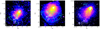 |
Fig. 1. Smoothed flux image of Abell 3411 combined from 1.2–4.0 keV XMM-Newton EPIC CCDs (left), 0.7–7.0 keV Suzaku XIS CCDs (middle), and 1.2–4.0 keV Chandra ACIS-I (right). Particle background and vignetting effect have been corrected. White contours are GMRT 610 MHz radio intensity. XMM-Newton and Suzaku analysis regions are plotted with cyan sectors. The locations of two BCGs are plotted with red crosses in the Chandra image. The coordinates of the BCGs are obtained from Golovich et al. (2019a). |
We extracted surface brightness profiles along four regions, which are marked on the XMM-Newton flux map in Fig. 1. The first selection region (the southwest region) is the previously reported shock (van Weeren et al. 2017). From the XMM-Newton flux map, this discontinuity is unlikely to be seen by the naked eye. With the help of the Chandra flux map, we are able to define an elliptical sector whose side is parallel to the discontinuity. The second region (south) is crossing the south discontinuity seen in the Chandra flux map (Andrade-Santos et al. 2019) as well as a diffuse radio emission. The third one (cold front) stretches along the direction of the bullet and probably hosts a bow shock. The last one is the bullet itself. We set the region boundary carefully to be parallel to the surface brightness edge.
We extracted surface brightness profiles from both XMM-Newton and Chandra datasets. We used a projected double power-law density model to fit discontinuities, whose unprojected density profile is
where C is the compression factor at the shock or cold front, and redge and nedge are the radius and the density at the edge, respectively. We assume the curvature radius along the line of sight is equal to the average radius of the surface brightness discontinuity (i.e. the ellipticity along the third axis is zero). The projected surface brightness profile is
where z is the coordinate along the line of sight, and Sbg is the surface brightness contributed by the X-ray background. For Chandra, we measure Sbg = 7 × 10⁻⁷ count s−1 cm−2 arcmin−2 from the front-illuminated ACIS-S chips. For XMM-Newton, this value is more difficult to properly estimate. Because soft protons are less vignetted than photons, we can see an artificial surface brightness increases beyond 10′. We therefore avoid regions located beyond 10′ from the focal point. C-statistics (Cash 1979) is adopted to calculate the likelihood function for fitting.
4. Spectral analysis
To study the thermodynamic structure of the cluster, in particular across known surface brightness discontinuities, we performed spectroscopic analysis and obtained the temperature from different selection regions. For spectral analysis, the spectral fitting package SPEX v3.05 (Kaastra et al. 1996, 2018) was used. The reference proto-solar element abundance table is from Lodders et al. (2009). OGIP format spectra and response matrices were converted to SPEX format by the trafo task. All spectra were optimally binned (Kaastra & Bleeker 2016) and fitted with C-statistics (Cash 1979). The Galactic hydrogen column density was calculated using the method of Willingale et al. (2013)4, which takes both atomic and molecular hydrogen into account. The weighted effective column density is nH = 5.92 × 1020 cm−2. We used the ROSAT All-Sky Survey (RASS) spectra generated by the X-Ray Background Tool5 (Sabol & Snowden 2019) to help us to constrain two foreground thermal components: the local hot bubble (LHB) and Galactic halo (GH). The RASS spectrum was selected from a 1° −2° annulus centred at our galaxy cluster. The two foreground components were modelled using single-temperature collisional ionisation equilibrium (CIE) models in SPEX. The GH is absorbed by the Galactic hydrogen while the LHB is unabsorbed. We fixed the abundance to the proto-solar abundance for those two components. The best-fit foreground parameters are shown in Table 3. These temperatures are consistent with previous studies (e.g. Yoshino et al. 2009).
4.1. XMM-Newton
In the XMM-Newton spectral analysis, the effective extraction region areas of spectra from different detectors were calculated using the SAS task backscale. To ensure that the extracted spectra from different detectors cover the same sky area, we excluded the union set of the bad pixels of all three detectors from each spectrum. This method leads to lower photon statistics but can reduce the spectral discrepancies due to different selection regions when we perform the parallel fitting. With the calculated backscale parameter, we determined the sky area of each spectrum with respect to 1 arcmin2 and set the region normalisation to that value. The spectral components and models are listed in Table 2. We fitted all spectra from different detectors simultaneously. We plot the MOS1 spectrum within r500 in Fig. 2 as an example to show all spectral components. The components of the MOS2 and pn spectra are similar, so we only additionally plot the fit residuals of these two detectors in Fig. 2.
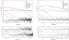 |
Fig. 2. r500XMM-Newton-EPIC MOS1 (top left) and Suzaku XIS0 (top right) spectra as well as individual spectral components. We also plot residuals from the other two EPIC detectors (bottom left) and XIS detectors (bottom right). The fit statistics are C − stat/d.o.f = 1992/1554 for XMM-Newton EPIC spectra and C − stat/d.o.f = 563/423 for Suzaku XIS spectra. |
Spectral fitting components and models.
X-ray foreground components constrained by the RASS spectrum.
The ICM is modelled with a single temperature CIE. The abundances of metal elements are coupled with the Fe abundance. With the FWC data, we find the particle background continuum can be fit by a broken power law with break energy at 2.5 and 2.9 keV for MOS and pn, respectively. Because the instrumental lines in particle backgrounds are spatially variable, we fitted instrumental lines as delta functions with free normalisations. The energies of instrumental lines are taken from Mernier et al. (2015). If the selection region includes MOS1 CCD4 or MOS2 CCD5 pixels, channels below 1.0 keV are ignored because of the low-energy noise plateau6. The two foreground components are coupled with the components of the RASS spectrum. To determine the point source detection limit and calculate the cosmic CXB flux, we first used the CIAO package tool wavdetect to detect point sources in a 1–8 keV combined XMM-Newton EPIC flux image. We set wavdetect parameters scale=“1.0 2.0 4.0”, ellsigma = 4, and sigthresh = 1e–5, which is roughly the reciprocal of the image size in our case. The values of other parameters were left as the default. In the detected source list, we selected the four lowest detection significance sources to extract and combined their MOS and pn spectra. The source extraction regions are directly obtained from the output of the wavdetect task. Local backgrounds were extracted and subtracted from the total source spectra with elliptical annuli, whose inner radii are the radii of the source regions, and the width is 15″. We fitted the point source spectra using abs * pow models with free power law normalisation and photon index. The best-fit flux in 2–8 keV range is (6.0 ± 0.5)×10−15 erg s−1 cm−2. Two out of four sources are in our Chandra point source catalogue (see Appendix C). Their Chandra fluxes are (6.8 ± 1.1)×10−15 and (9.2 ± 1.2)×10−15 erg s−1 cm−2, respectively. Therefore, we used 6.0 × 10⁻¹⁵ erg s−1 cm−2 from 2–8 keV as a detection limit to calculate the CXB surface brightness. The corresponding CXB surface brightness is 3.5 × 10⁻¹⁴ erg s−1 cm−2 arcmin−2 with a fixed photon index Γ = 1.41; see Appendix C for details. The CXB deviation is calculated by Eq. (C.5); we fitted spectra with ±1σsys CXB luminosity to obtain the systematic errors contributed by CXB uncertainty. We also included the GH systematic error for XMM-Newton spectral analysis with the uncertainty measured from the Suzaku offset observation (see Sect. 4.2.1). We calibrated the soft proton background in terms of spectral models and vignetting functions with an observation of the Lockman Hole (see Appendix B). The best-fit parameters and the systematic uncertainties of each soft proton component are listed in Table B.3. When studying the systematics from the soft proton components, we fit spectra with ±1σsys of the MOS1, MOS2, and pn soft proton luminosity individually. The envelope of the highest and the lowest fitted temperatures are taken as the systematics from the soft proton model.
4.2. Suzaku
In the Suzaku spectral analysis, the energy range 0.7–7.0 keV is used for spectral fitting. Auxiliary response files (ARFs) are generated by the task xissimarfgen (Ishisaki et al. 2007) with the parameter source_mode=UNIFORM. X-ray spectral components are the same as those of the EPIC spectra. We exclude sources with 2–8 keV flux S2 − 8 keV > 2 × 10⁻¹⁴ erg s−1 cm−2 in our catalogue (see Appendix C) using 1′ radius circles. The unresolved CXB flux, as well as its uncertainty for each selected region, were calculated using Eq. (C.5). All spectra from different detectors were fitted simultaneously as well. Because the Suzaku ARFs are normalised to 400π arcmin2, we set region normalisations in SPEX to 400π. In that case, the fitted luminosity value corresponds to 1 arcmin2. An example of the XIS0, the r500 spectrum is shown in Fig. 2 to illustrate all spectral components. As in the EPIC spectra, we additionally plot the residuals of XIS1 and XIS3.
4.2.1. Offset observation
We used the offset observation to study the systematic error from the foreground X-ray components. We extracted spectra from the full FOV but excluded the XIS0 bad region and point sources by visual inspection. We fitted the spectrum from 0.4 to 7.0 keV with LHB, GH, and CXB components. Additionally, we added a delta line component at 0.525 keV to fit an extremely strong O I Kα line, which is generated by the fluorescence of solar X-rays with neutral oxygen in the Earth’s atmosphere (Sekiya et al. 2014). Because the LHB flux is prominent at energies much lower than 0.4 keV, we still coupled the normalisation and temperature with the RASS LHB component. From 0.4 to 1 keV, the spectrum is dominated by the GH. We freed the normalisation of the GH but still coupled the temperature with the RASS GH component. The CXB power law index was set as Γ = 1.41, and the normalisation was thawed. Best-fit parameters are listed in Table 4. The best-fit GH normalisation is 40% lower than the best-fit value from RASS. We include the 40% GH normalisation to study the systematic error.
Best-fit parameters of Suzaku offset spectra.
4.2.2. Selection regions
Because of the large radius of the point spread function (PSF) of Suzaku, structures on small scales are not resolved. We use sector regions centred at the centre of the cluster and extending towards the southeast (SE), south (S), and southwest (SW) directions (see Fig. 1) to extract spectra and measure the temperature profiles.
4.3. XMM-Newton-Suzaku cross-calibration
Because Suzaku XIS has a lower instrumental background and does not suffer from soft proton contamination due to its low orbit, its temperature measurements in faint cluster outskirts can be considered more reliable than those from XMM-Newton EPIC. Therefore, we used the Suzaku temperature profiles to cross-check the validity of the XMM-Newton temperature profile and verify our soft proton modelling approach. We used the Suzaku SE selection region for the cross-check because the S and SW regions cover the missing MOS1 CCD. We extracted EPIC spectra from the exact same regions as the XIS spectra except for the point-source exclusion regions. All spectra were fitted using the method described in Sects. 4.1 and 4.2. We plot Suzaku and XMM-Newton temperature profiles as well as profiles from only MOS and pn in Fig. 3. Except for the second subregion from the cluster centre, the MOS temperatures are globally higher than Suzaku XIS temperatures, which are themselves higher than pn temperatures. The total EPIC temperatures are in agreement with XIS temperatures within the systematic errors.
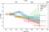 |
Fig. 3. Temperature profiles of both Suzaku and XMM-Newton in the Suzaku SE selection region. Filled bands of each profile represent the major systematic errors, i.e. SP for XMM-Newton and CXB+GH for Suzaku. |
5. Results
We performed both imaging and spectral analysis for surface brightness discontinuities. We measured the global temperature of the cluster. Meanwhile, we obtained temperature profiles to the cluster outskirts using the Suzaku data.
5.1. Properties of surface brightness discontinuities
We calculate surface brightness profiles from each selection region shown in Fig. 1. We use the double power law model introduced in Sect. 3 to fit surface brightness profiles. Because Chandra has a narrow PSF, we first fit Chandra profiles to obtain precise redges. For XMM-Newton profiles, we convolve a σ = 0.1′ Gaussian kernel to the model to mimic the PSF effect. We fix redge for the XMM-Newton profile fitting based on the value determined with Chandra. We compare the C-statistic value when fixing C to the Chandra result or allowing it to be free in the fit.
Surface brightness profiles and fitted models are plotted in Fig. 4, and fitted parameter values as well as fitting statistics are listed in Table 5. There is a systematic offset between the density jumps measured with Chandra and XMM-Newton. We use the best-fit redge as the location of the shock/cold front to extract spectra. We also split both the high and low-density sides into several bins when extracting spectra. Temperature profiles are plotted in Fig. 5.
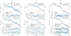 |
Fig. 4. Surface brightness profile fitting results of SE, S, and cold front (CF) regions. Upper panel: Chandra surface brightness. Lower panel: XMM-Newton surface brightness profile fitted by fixed and free C parameters. All XMM-Newton models are smoothed by a σ = 0.1′ Gaussian function. Red lines indicate the ratio between the subtracted FWC background counts and the remaining signal, which include the ICM, X-ray background, and soft proton contamination. In regions where this ratio is higher than one, the FWC background dominates. Black dashed lines are the radio surface brightness profiles in an arbitrary unit. |
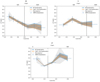 |
Fig. 5. XMM-Newton temperature profile of each region. Dashed lines indicate edge locations fitted from surface brightness profiles. Grey bands indicate the temperature discrepancy between MOS and pn. |
5.1.1. Southeast
At the previously reported shock front, the compression factor fitted with our selection region from the Chandra profile is identical to the result of van Weeren et al. (2017), namely C = 1.3 ± 0.1, and is slightly higher than the result of Andrade-Santos et al. (2019),  , but within 1σ uncertainty. However, it is hard to find this feature in the XMM-Newton profile. Fitting with fixed redge and C, we obtain C-stat/d.o.f = 76.4/44. If we free the C parameter, the fitted CXMM − Newton = 1.09 ± 0.08, which means the data are consistent with the lack of a density jump, but are consistent with the result of Andrade-Santos et al. (2019). The reason that we do not detect an edge in the XMM-Newton profile could be the missing pixels around the edge. The radio relic is located very close to bad pixel columns of MOS2, and a CCD gap of pn. The temperature profile (the top-left panel in Fig. 5) drops linearly and then flattens at larger radii. The temperature at the bright side of the edge is higher than at the other side. Hence, we rule out the possibility that this edge is a cold front.
5.1.2. South
In the southern region, a significant surface brightness jump is seen in both Chandra (CChandra = 1.74 ± 0.15) and XMM-Newton (CXMM − Newton = 1.45 ± 0.10) profiles. A simple spherically symmetric double power-law density model cannot fit the Chandra profile perfectly; it is a sudden jump with flat or even increasing surface brightness profile on the high-density side. There is an excess above the best-fit model at the edge. The temperature is almost identical across the edge, which is not a typical shock or cold front. We discuss this edge in Sect. 6.3.
5.1.3. Cold front
The cold front surface brightness profile can be well modelled by the double power-law density model. The density ratio from Chandra observation CChandra = 2.00 ± 0.06 is higher than that from the XMM-Newton, which is CXMM − Newton = 1.74 ± 0.05. Similar to the southern edge, even if we account for the PSF of XMM-Newton, the density jump measured by XMM-Newton is smaller than that determined using Chandra. In addition, the inner power-law component of the density profiles is steeper when measured with XMM-Newton than with Chandra. The energy dependence of the vignetting function and of the effective area (and their uncertainties) can affect this inner slope, which in turn is correlated with the density jump (a steeper inner power-law leads to a smaller compression factor). This may contribute to the observed differences. The temperature profile confirms that it is a cold front. The temperature reaches the minimum before the cold front and then rises until r = 3′.
5.2. Global temperature
We extract spectra from the region with r500 = 1.3 Mpc (Andrade-Santos et al. 2019) to obtain the global temperature. Although we miss MOS1 CCD3 and 6, most of the flux is in the centre CCD, which means our result will not be significantly biased by the missing CCDs. The best-fit temperature is kT500 = 4.84 ± 0.04 ± 0.19 keV, where the second error item represents the systematic uncertainty. The temperatures of individual detectors are listed in Table 6. The kT500, MOS is about 0.1 keV higher than kT500, pn. These two measurements agree within their 1σ uncertainty interval, which is dominated by the systematic error from the soft proton model. Compared with the result of Andrade-Santos et al. (2019) of kT500 = 6.5 ± 0.1 keV, the kT500 in our work is much lower.
kT500 from XMM-Newton and Suzaku.
We also used Suzaku data to check the global temperature. Suzaku does not suffer from soft proton contamination, and its NXB level is lower than that of XMM-Newton, making it a valuable tool to check our XMM-Newton analysis. The Suzaku observation does not cover the whole r500 area. To avoid the missing XIS0 strip, we extract spectra from the south semicircle (see the red region in Fig. 6). The best-fit results with all detectors as well as with the only front-illuminated (FI, XIS0 + XIS3) and back-illuminated (BI, XIS1) CCDs are listed in Table 6. The best-fit temperature is kT500 = 5.17 ± 0.07 ± 0.13 keV, which is slightly higher than the XMM-Newton result.
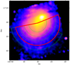 |
Fig. 6. Suzaku semicircle r500 selection region (red) and radial bins (green). |
5.3. Temperature profiles to the outskirts
Individual Suzaku temperature profiles of three sectors are shown in Fig. 7. Apart from three individual directions, we split the Suzakur500 region into four annuli (the green regions in Fig. 6), and define another bin outside of r500. We plot all four profiles together with a typical relaxed cluster outskirt temperature profile (Burns et al. 2010), where we take ⟨kT⟩ = 5.2 keV. The curve obtained by these latter authors agrees with Suzaku observations of relaxed clusters remarkably (Akamatsu et al. 2011; Reiprich et al. 2013). For our data, at r500, the southern temperature profile agrees with the profile of Burns et al. (2010). The other three profiles are marginally higher than the typical relaxed cluster temperature profile but within 1σ systematic error. In the work of Burns et al. (2010), ⟨kT⟩ is the averaged temperature between 0.2 and 2.0 r200. Because our Suzaku observation only covers the r500 area, the actual ⟨kT⟩ could be slightly lower than the value we use. In that case, the southern temperature profile could also be marginally higher than the profile of Burns et al.. This cluster is undergoing a major merger, and our results show that the temperature in the outskirts has been disturbed.
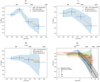 |
Fig. 7. Suzaku temperature profiles of the SE, S, and SW regions, as well as a comparison with the relaxed temperature profile in the outskirts predicted by numerical simulations. |
6. Discussion
6.1. T500 discrepancy
Our measurements of kT500 are lower than the result of Chandra data. The cross-calibration uncertainties between XMM-Newton EPIC and Chandra ACIS may be the major cause for this discrepancy. Using the scaling relation of temperatures between EPIC and ACIS log kTEPIC = 0.0889 × log kTACIS (Schellenberger et al. 2015), a 6.5 keV ACIS temperature corresponds to a 5.3 keV EPIC temperature, which is close to our measurement. By contrast, the temperature discrepancy between XMM-Newton EPIC and Suzaku XIS is relatively small. This discrepancy of 8% is slightly larger than the value from the Suzaku XIS and XMM-Newton EPIC-pn cross-calibration study (5%, Kettula et al. 2013). Because the Suzaku extraction region does not cover the cold front, the reported Suzaku temperature may be higher than the average value within the entire r500 region, explaining this difference.
With our temperature results, we use the M500 − kTX relation h(z)M500 = 1014.58 × (kTX/5.0)1.71 M⊙ (Arnaud et al. 2007) to roughly estimate the mass of the cluster. The kTX is the temperature from 0.1 to 0.75r500. We do not exclude the inner 0.1r500 part because it is not a relaxed system, and there is no dense cool core in the centre. For kTX = 5.0 keV, the M500 − TX relation suggests a mass of M500 = 5.1 × 10¹⁴ M⊙. This is less than that from the Planck Sunyaev–Zeldovich catalogue of MSZ = (6.6 ± 0.3)×1014 M⊙ (Planck Collaboration XXVII 2016). However, this underestimation is not surprising. Because the source is undergoing a major merger, the kinetic energy of two sub-halos is still being dissipated into the thermal energy of the ICM. Once the system relaxes, the kTX will be higher than in the current epoch.
6.2. Shock properties
The shock Mach number can be calculated by the Rankine-Hugoniot condition (Landau & Lifshitz 1959) either from the density jump or from the temperature jump,
![$$ \begin{aligned} \mathcal{M}&=\left[\frac{2C}{\gamma +1-C(\gamma -1)}\right]^2\end{aligned} $$](/articles/aa/full_html/2020/10/aa37965-20/aa37965-20-eq6.gif)
where C is the compression factor across the shock, and γ = 5/3 if we assume the ICM is an ideal gas. Because the systematic errors from the CXB and GH are Gaussian, we directly propagate them into the statistical error when estimating the Mach number uncertainty. However, the soft proton systematic uncertainty is not Gaussian, and so we use the measured temperature and the temperature obtained by varying the soft proton component within their ±1σ uncertainties determined in Appendix B to estimate the XMM-Newton Mach number systematic error.
The Suzaku southeast sector covers the re-acceleration site, and we see a jump from the second to the third point in that temperature profile. The Suzaku spectral extraction regions are defined unbiasedly. We further inspect the temperature profile based on the radio morphology. The radio-based selection region is shown in Fig. 8. We intentionally leave a 1.1′ gap (Akamatsu et al. 2015) between the second and the third bin to avoid photon leakage from the brighter side. We plot both the XMM-Newton and Suzaku temperature profiles of this sector in Fig. 9. Because XMM-Newton has a much smaller PSF than Suzaku, we can use the spectrum from the gap.
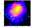 |
Fig. 8. Suzaku flux map and the cyan spectral extraction regions are based on radio morphology (white contours). |
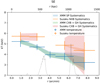 |
Fig. 9. Suzaku and XMM-Newton temperature profiles from the radio-based selection regions in Fig. 8. The radio surface brightness profile is plotted as a black line. |
There is a systematic offset between Suzaku and XMM-Newton. The Suzaku temperature is globally higher than the XMM-Newton temperature. Both profiles drop from the centre of the cluster to the outskirts. The new XMM-Newton temperature profile is similar to the previous one in Sect. 5.1.1. The temperature decreases from the centre of the cluster and flattens after the radio relic. We use temperatures across the radio relic to obtain the shock Mach number. As a comparison, we calculate the Mach number by the density jump fitted from the Chandra surface brightness profile. Results are listed in Table 7. From our spectral analysis, we confirm the Mach number of this shock is close to the value measured from the surface brightness profile fit. Results from all telescopes point to the value ℳX ∼ 1.2. This shock is another case where the radio Mach number is higher than the X-ray Mach number (see Fig. 10). Such a low Mach number supports the re-acceleration scenario. We note that our calculation does not account for the presence of a “relaxed” temperature gradient in the absence of a shock. This could further reduce the Mach number, but the conclusion that the re-acceleration mechanism is needed would remain robust.
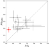 |
Fig. 10. Shock Mach numbers derived from radio spectral index (ℳRadio) against those from the ICM temperature jump (ℳX). The data points of previous studies (grey) are adapted from Fig. 22 in van Weeren et al. (2019). The red point is the southwestern shock in Abell 3411-3412. |
Comparison of the southeast shock Mach number obtained from different instruments and methods.
6.3. The mystery of the southern edge
The density jump at the southern edge is strong, and Andrade-Santos et al. (2019) claim it is a cold front from the sub-cluster Abell 3412. From our spectral fitting, the temperature inside and outside of the southern edge is kT = 4.36 ± 0.34 keV, and kT = 4.26 ± 0.46 keV, respectively. The projected temperature jump is 1.02 ± 0.14. From the surface brightness fitting, the de-projected density jump is C = 1.7 ± 0.2. This value corresponds to a de-projected temperature jump of 1.48 ± 0.25 under the assumption of Rankine-Hugoniot shock conditions, and a temperature jump 0.59 ± 0.07 under the assumption that it is a cold front in pressure equilibrium. Neither the shock scenario nor the cold front scenario matches the measured lack of temperature jump.
To obtain the de-projected temperature jump, we simply assume that the spectrum from the high-density side is a double-temperature spectrum. The temperature of one of the components is the same as that from the low-density side. We assume that the discontinuity structure is spherically symmetric, and calculate the volume ratio between the intrinsic and projected components in the high-density side. We fit spectra from both sides simultaneously. For the high-density side spectrum, we couple one CIE temperature to that of the low-density spectrum. We also couple the normalisation of that component to that of the low-density spectrum with a factor of the volume ratio. We leave the other two temperature and normalisation parameters free. The de-projected temperature ratio is then 1.08 ± 0.17 with a systematic uncertainty 0.10. This value is ∼1.3σ offset from the shock scenario but is ∼2.6σ offset from the cold front scenario. Therefore, the temperature jump we measured is in closer agreement with the shock scenario. Also, the pressure across the edge is out of equilibrium. The pressure jump implies a supersonic motion of the gas.
The presence of a huge density jump but a marginal temperature jump suggests an excess of surface brightness on the bright side of the edge. Also, the Chandra surface brightness profile shows a tip beyond the best-fit double power-law density model. Because the brightest cluster galaxy (BCG) of Abell 3412 (see Fig. 1) is located only 1′ away from the southern edge, the surface brightness excess may be due to the remnant core of the sub-cluster Abell 3412. We are therefore looking at a more complex superposition of a core and a shock. The second possibility is that the excess emission may be associated with one galaxy in the cluster, which contains highly ionised gas. The gas is being stripped from the galaxy while it moves in the cluster (e.g. ESO 137-001 Sun et al. 2006). A third possibility is that the excess emission could be inverse Compton (IC) radiation from the radio jet tail on top of the X-ray edge. We estimate the upper limit of IC emission based on the equation from Brunetti & Jones (2014):
where  is the emission-weighted magnetic field strength and ℓ(α) is a dimensionless function. In Abell 3411, the radio spectral index at the southern edge is α ∼ 1 (van Weeren et al. 2017), at which ℓ = 3.16 × 10³. In the third southern spectral extraction region, the averaged radio flux at 325 MHz is 1.2 × 10⁻³ Jy arcmin−2. Usually, in the ICM, the magnetic field value B is approximately equal to between one and a few μG. If we use ⟨B⟩ = 1 μG to estimate the upper limit of the X-ray IC flux, the corresponding flux density is 3.24 × 10⁻²⁴ erg s−1 Hz−1 cm−2 arcmin−2. The converted photon density is 7.8 × 10⁻⁹ ph s−1 keV−1 cm−2 arcmin−2 at 1 keV. In the 1.2–4.0 keV band, the contribution of the IC emission is 2.8 × 10⁻⁸ ph s−1 cm−2 arcmin−2, which is about two orders of magnitude lower than the total source flux. This possibility is therefore ruled out.
6.4. The location of the bow shock
In front of the bullet, Andrade-Santos et al. (2019) claim the detection of a bow shock with  at
at  arcmin. The significance of the density jump is low and the uncertainty of the location is large. To confirm this jump, we extract the XMM-Newton surface brightness profile in front of the bullet using the same region definition as that used by Andrade-Santos et al. (2019) (see Fig. 11). We fit the profile using both single power-law and double power-law models. The double power-law model returns C-stat/d.o.f. = 98.4/115 with density jump C = 1.056 ± 0.061. As a comparison, the single power-law model returns C-stat/d.o.f. = 99.8/118. A single power-law model can fit this profile well.
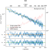 |
Fig. 11. XMM-Newton surface brightness profile of the northwest region. No density jump is found. |
So far, radio observation cannot pinpoint the bow shock because this cluster has neither a radio relic nor a radio halo edge in the northern outskirts. One other method to predict the bow shock location is to use the relation between the bow shock stand-off distance and the Mach number (Sarazin 2002; Schreier 1982). However, Dasadia et al. (2016) found that most of the bow shocks in galaxy clusters have longer stand-off distances than the expected value. In extreme cases, such as that of Abell 2146 (Russell et al. 2010), the difference can reach a factor of ten (Dasadia et al. 2016). Recently, from simulations, Zhang et al. (2019) found that the unexpectedly large stand-off distance can be due to de-acceleration of the cold front speed after the core passage, while the shock front can move faster.
The offset between the projected BCG (see Fig. 1) and the X-ray peak positions implies the merging phase. For the sub-cluster Abell 3411, the BCG lags behind the X-ray peak by ∼17″. Without a weak-lensing observation, we consider the position of the BCG as the bottom of the gravitational potential well of the dark matter halo. When two sub-clusters undergo the first core passage, the position of the dark matter halo will usually be in front of the gas density peaks (e.g. the Bullet cluster, Clowe et al. 2006) because dark matter is collision-less, but the ICM is collisional. When the dark matter halo reaches the apocentre, the ambient gas pressure drops quickly and so the gas can catch up and overtake the mass peak (e.g. Abell 168, Hallman & Markevitch 2004). Hence, the location of the BCG of Abell 3411 indicates the dark matter halo has almost reached its apocentre. The dynamic analysis also suggests the two sub-clusters are near their apocentres (van Weeren et al. 2017). Thus, the stand-off distance could be much larger than the expected value. The stand-off distance calculated from the bow shock location reported by Andrade-Santos et al. (2019) almost matches the Mach number ℳ ∼ 1.2. We speculate that the real bow shock location could be far ahead of the reported location. Unfortunately, in the northwestern outskirts, the XMM-Newton counts are dominated by the background, and the Suzaku observation does not cover that region. We are unable to probe the bow shock by thermodynamic analysis.
7. Conclusion
We analyse the XMM-Newton and Suzaku data to study the thermodynamic properties of the merging system Abell 3411-3412. We calibrate the XMM-Newton soft proton background properties based on one Lockman hole observation and apply the model to fit the Abell 3411 spectra (Appendix B). Our work is an update of the current understanding of this merging system. We summarise our results as follows:
-
We measure T500 = 4.84 ± 0.04 ± 0.19 with XMM-Newton and T500 = 5.17 ± 0.07 ± 0.13 in the southern semicircle with Suzaku. The corresponding mass from the M500 − TX relation is M500 = 5.1 × 10¹⁴ M⊙.
-
The Chandra northern bullet-like sub-cluster and southern edges are detected by XMM-Newton as well, while the southeastern edge shows no significant density jump in the XMM-Newton surface brightness profile.
-
The southern edge was claimed as a cold front previously (Andrade-Santos et al. 2019). With our XMM-Newton analysis, the temperature jump prefers a shock front scenario. There is a clear pressure jump indicating supersonic motions, although the geometry seems to be more complicated, with a possible superposition of a shock and additional stripped material from the Abell 3412 sub-cluster.
-
Both Suzaku and XMM-Newton results confirm the southeastern edge is a ℳ ∼ 1.2 shock front, which agrees with the previous result from Chandra surface brightness fit (van Weeren et al. 2017; Andrade-Santos et al. 2019). Such a low Mach number supports the particle re-acceleration scenario at the shock front.
Acknowledgments
We thank the anonymous referee for constructive suggestions that improved this paper. X.Z. is supported by the the China Scholarship Council (CSC). R.J.vW. acknowledges support from the ERC Starting Grant ClusterWeb 804208. SRON is supported financially by NWO, The Netherlands Organization for Scientific Research. This research made use of Astropy (http://www.astropy.org), a community-developed core Python package for Astronomy (Astropy Collaboration 2013, 2018). This research is based on observations obtained with XMM-Newton, an ESA science mission with instruments and contributions directly funded by ESA Member States and NASA. This research has made use of data obtained from the Suzaku satellite, a collaborative mission between the space agencies of Japan (JAXA) and the USA (NASA). This research has made use of data obtained from the Chandra Data Archive and the Chandra Source Catalog, and software provided by the Chandra X-ray Center (CXC) in the application package CIAO.2pt
References
- Akamatsu, H., Hoshino, A., Ishisaki, Y., et al. 2011, PASJ, 63, S1019 [CrossRef] [Google Scholar]
- Akamatsu, H., van Weeren, R. J., Ogrean, G. A., et al. 2015, A&A, 582, A87 [Google Scholar]
- Akamatsu, H., Mizuno, M., Ota, N., et al. 2017, A&A, 600, A100 [NASA ADS] [CrossRef] [EDP Sciences] [Google Scholar]
- Andrade-Santos, F., van Weeren, R. J., Di Gennaro, G., et al. 2019, ApJ, 887, 31 [CrossRef] [Google Scholar]
- Arnaud, M., Pointecouteau, E., & Pratt, G. W. 2007, A&A, 474, L37 [NASA ADS] [CrossRef] [EDP Sciences] [Google Scholar]
- Astropy Collaboration (Price-Whelan, A. M., et al.) 2018, AJ, 156, 123 [Google Scholar]
- Astropy Collaboration (Robitaille, T. P., et al.) 2013, A&A, 558, A33 [NASA ADS] [CrossRef] [EDP Sciences] [Google Scholar]
- Blandford, R., & Eichler, D. 1987, Phys. Rep., 154, 1 [Google Scholar]
- Brunetti, G., & Jones, T. W. 2014, Int. J. Mod. Phys. D, 23, 1430007 [Google Scholar]
- Burns, J. O., Skillman, S. W., & O’Shea, B. W. 2010, ApJ, 721, 1105 [Google Scholar]
- Cash, W. 1979, ApJ, 228, 939 [NASA ADS] [CrossRef] [Google Scholar]
- Cavaliere, A., & Fusco-Femiano, R. 1976, A&A, 500, 95 [NASA ADS] [Google Scholar]
- Clowe, D., Bradač, M., Gonzalez, A. H., et al. 2006, ApJ, 648, L109 [NASA ADS] [CrossRef] [Google Scholar]
- Dasadia, S., Sun, M., Morandi, A., et al. 2016, MNRAS, 458, 681 [NASA ADS] [CrossRef] [Google Scholar]
- Ensslin, T. A., Biermann, P. L., Klein, U., & Kohle, S. 1998, A&A, 332, 395 [NASA ADS] [Google Scholar]
- Finoguenov, A., Sarazin, C. L., Nakazawa, K., Wik, D. R., & Clarke, T. E. 2010, ApJ, 715, 1143 [NASA ADS] [CrossRef] [Google Scholar]
- Giovannini, G., Vacca, V., Girardi, M., et al. 2013, MNRAS, 435, 518 [NASA ADS] [CrossRef] [Google Scholar]
- Golovich, N., Dawson, W. A., Wittman, D. M., et al. 2019a, ApJS, 240, 39 [NASA ADS] [CrossRef] [Google Scholar]
- Golovich, N., Dawson, W. A., Wittman, D. M., et al. 2019b, ApJ, 882, 69 [Google Scholar]
- Hallman, E. J., & Markevitch, M. 2004, ApJ, 610, L81 [NASA ADS] [CrossRef] [Google Scholar]
- Hickox, R. C., & Markevitch, M. 2006, ApJ, 645, 95 [NASA ADS] [CrossRef] [Google Scholar]
- Hoshino, A., Henry, J. P., Sato, K., et al. 2010, PASJ, 62, 371 [NASA ADS] [CrossRef] [Google Scholar]
- Ishisaki, Y., Maeda, Y., Fujimoto, R., et al. 2007, PASJ, 59, 113 [NASA ADS] [Google Scholar]
- Jones, F. C., & Ellison, D. C. 1991, Space Sci. Rev., 58, 259 [NASA ADS] [CrossRef] [Google Scholar]
- Kaastra, J. S., & Bleeker, J. A. M. 2016, A&A, 587, A151 [NASA ADS] [CrossRef] [EDP Sciences] [Google Scholar]
- Kaastra, J. S., Mewe, R., & Nieuwenhuijzen, H. 1996, UV and X-ray Spectroscopy of Astrophysical and Laboratory Plasmas, 411 [Google Scholar]
- Kaastra, J. S., Raassen, A. J. J., de Plaa, J., & Gu, L. 2018, SPEX X-ray Spectral Fitting Package [Google Scholar]
- Kang, H. 2015, J. Korean Astron. Soc., 48, 9 [NASA ADS] [CrossRef] [Google Scholar]
- Kang, H., & Jones, T. W. 2002, J. Korean Astron. Soc., 35, 159 [NASA ADS] [CrossRef] [Google Scholar]
- Kang, H., & Jones, T. W. 2005, ApJ, 620, 44 [NASA ADS] [CrossRef] [Google Scholar]
- Kang, H., Jones, T. W., & Gieseler, U. D. J. 2002, ApJ, 579, 337 [NASA ADS] [CrossRef] [Google Scholar]
- Kang, H., & Ryu, D. 2011, ApJ, 734, 18 [NASA ADS] [CrossRef] [Google Scholar]
- Kardashev, N. S. 1962, Soviet Ast., 6, 317 [Google Scholar]
- Kettula, K., Nevalainen, J., & Miller, E. D. 2013, A&A, 552, A47 [NASA ADS] [CrossRef] [EDP Sciences] [Google Scholar]
- Kuntz, K. D., & Snowden, S. L. 2008, A&A, 478, 575 [NASA ADS] [CrossRef] [EDP Sciences] [Google Scholar]
- Landau, L. D., & Lifshitz, E. M. 1959, Fluid mechanics (Pergamon Press) [Google Scholar]
- Lehmer, B. D., Xue, Y. Q., Brandt, W. N., et al. 2012, ApJ, 752, 46 [NASA ADS] [CrossRef] [Google Scholar]
- Lodders, K., Palme, H., & Gail, 2009, 4.4 Abundances of the elements in the Solar System: Datasheet from Landolt-Börnstein - Group VI Astronomy and Astrophysics · Volume 4B: “Solar System” in Springer Materials [Google Scholar]
- Markevitch, M., & Vikhlinin, A. 2007, Phys. Rep., 443, 1 [NASA ADS] [CrossRef] [EDP Sciences] [Google Scholar]
- Markevitch, M., Govoni, F., Brunetti, G., & Jerius, D. 2005, ApJ, 627, 733 [NASA ADS] [CrossRef] [Google Scholar]
- Mernier, F., de Plaa, J., Lovisari, L., et al. 2015, A&A, 575, A37 [Google Scholar]
- Planck Collaboration XXVII. 2016, A&A, 594, A27 [NASA ADS] [CrossRef] [EDP Sciences] [Google Scholar]
- Reiprich, T. H., Basu, K., Ettori, S., et al. 2013, Space Sci. Rev., 177, 195 [NASA ADS] [CrossRef] [EDP Sciences] [Google Scholar]
- Rosen, S. R., Webb, N. A., Watson, M. G., et al. 2016, A&A, 590, A1 [NASA ADS] [CrossRef] [EDP Sciences] [Google Scholar]
- Russell, H. R., Sanders, J. S., Fabian, A. C., et al. 2010, MNRAS, 406, 1721 [Google Scholar]
- Sabol, E. J., & Snowden, S. L. 2019, sxrbg: ROSAT X-Ray Background Tool [Google Scholar]
- Sarazin, C. L. 2002, The Physics of Cluster Mergers, eds. L. Feretti, I. M. Gioia, & G. Giovannini, Astrophys. Space Sci. Libr., 272, 1 [Google Scholar]
- Schellenberger, G., Reiprich, T. H., Lovisari, L., Nevalainen, J., & David, L. 2015, A&A, 575, A30 [NASA ADS] [CrossRef] [EDP Sciences] [Google Scholar]
- Schreier, S. 1982, Compressible Flow, AWiley-Interscience publication(Wiley) [Google Scholar]
- Sekiya, N., Yamasaki, N. Y., Mitsuda, K., & Takei, Y. 2014, PASJ, 66, L3 [CrossRef] [Google Scholar]
- Serlemitsos, P. J., Soong, Y., Chan, K.-W., et al. 2007, PASJ, 59, S9 [NASA ADS] [Google Scholar]
- Stroe, A., Shimwell, T., Rumsey, C., et al. 2016, MNRAS, 455, 2402 [NASA ADS] [CrossRef] [Google Scholar]
- Sun, M., Jones, C., Forman, W., et al. 2006, ApJ, 637, L81 [NASA ADS] [CrossRef] [Google Scholar]
- Tawa, N., Hayashida, K., Nagai, M., et al. 2008, PASJ, 60, S11 [NASA ADS] [Google Scholar]
- van Weeren, R. J., Fogarty, K., Jones, C., et al. 2013, ApJ, 769, 101 [NASA ADS] [CrossRef] [Google Scholar]
- van Weeren, R. J., Andrade-Santos, F., Dawson, W. A., et al. 2017, Nat. Astron., 1, 0005 [NASA ADS] [CrossRef] [Google Scholar]
- van Weeren, R. J., de Gasperin, F., Akamatsu, H., et al. 2019, Space Sci. Rev., 215, 16 [NASA ADS] [CrossRef] [Google Scholar]
- Wang, S., Liu, J., Qiu, Y., et al. 2016, ApJS, 224, 40 [NASA ADS] [CrossRef] [Google Scholar]
- Willingale, R., Starling, R. L. C., Beardmore, A. P., Tanvir, N. R., & O’Brien, P. T. 2013, MNRAS, 431, 394 [NASA ADS] [CrossRef] [Google Scholar]
- Yoshino, T., Mitsuda, K., Yamasaki, N. Y., et al. 2009, PASJ, 61, 805 [NASA ADS] [Google Scholar]
- Zhang, C., Churazov, E., Forman, W. R., & Jones, C. 2019, MNRAS, 482, 20 [NASA ADS] [CrossRef] [Google Scholar]
Appendix A: Light curves of EPIC CCDs
In Table 1, the MOS2 GTI is about 8 ks larger than MOS1. We plot the light curve and filtered GTIs of each EPIC detector in Fig. A.1. Although the light curves of two MOS detectors show a similar trend, some flares are only significant in MOS1. This explains why we obtain less GTI for MOS1.
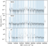 |
Fig. A.1. Inside FOV light curves for the three EPIC detectors in the 10–12 keV band with 100s bins. The filtered GTIs are shown as blue shadows. |
Out-of-FOV detector pixels are usually used for particle background level estimation. However, the out-of-FOV corners of the EPIC-pn CCD suffer from soft proton flares as well. We select 100s binned pn out-of-FOV light curves with selection criteria FLAG==65536 && PATTERN==0 && (PI IN [10000:12000]). To make a comparison, we extract light curves of the two MOS CCDs with the same out-of-FOV region expressions as in Sect. 2, which are from Kuntz & Snowden (2008). Light curves are plotted in Fig. A.2. We use a two-sample Kolmogorov-Smirnov (KS) test to check whether the cumulative density function (CDF) of the count rate matches a Poisson distribution. For the pn CCD, the p-value is less than 0.05. Therefore, the null hypothesis that the count rate follows a Poisson distribution is rejected. The KS test suggests that the out-of-FOV region of the pn detector is significantly contaminated by soft proton flares, while the out-of-FOV of the MOS area is clean enough to be used as a reference for the particle background level estimation.
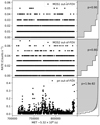 |
Fig. A.2. Out-of-FOV 10–12 keV light curves of three EPIC detectors. Right panels: CDFs of count rates. For each light curve, the CDF of the Poisson distribution with μ from the data is plotted as a grey area. The p-values to reject the null hypothesis that the count rate distribution is Poissonian are labelled. |
Appendix B: Soft proton modelling
Our observation suffered from significant soft proton contamination. Although we adopt strict flare filtering criteria, the contamination in the quiescent state is not negligible. Inappropriate estimations of the soft proton flux, as well as its spectral shape, would introduce considerable systematic error to fit the results. The integrated flare state soft proton spectra from MOS are studied by Kuntz & Snowden (2008). They are smooth and featureless, with the shape of an exponential cut-off power law. The spectrum is harder when flares are stronger.
The soft proton spectra of pn during flares have not been studied yet. To investigate the soft proton background properties, including spectral parameters, vignetting functions, and so on, we analyse one observation of the Lockman Hole (ObsID: 0147511201), which is also heavily contaminated by soft proton flares. That observation was also performed with the medium filter. Flare state time intervals are defined by μ + 2σ filtering criteria on 100 s binned light curves in the 10–12 keV energy intervals. The flare state proportion of pn is ∼87%. The pure flare state spectra are simply calculated by subtracting quiescent state spectra from flare state spectra.
B.1. Spectral analysis
Flare state soft proton spectra in the 0.5–14.0 keV band within a 12′ radius are plotted in Fig. B.1. The spectra of the centre and outer MOS CCDs are plotted individually. The shape of the pn spectrum is almost coincident with that of MOS; they are all smooth and featureless and can be described as a cut-off power law. The spectra from central MOS CCDs are coincident with each other. However, the spectra from outer CCDs are slightly different.
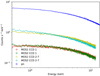 |
Fig. B.1. Flare state soft proton spectra in 12′ radius. |
Redistribution matrix files (RMFs) generated by rmfgen are calibrated on photons and include the photon redistribution jump at the Si K edge. However, we do not see any feature there in the soft proton spectra. As a result, we use genrsp in FTOOL to generate a dummy RMF for fitting. A SPEX built-in generalised power-law model is used to model the soft proton spectra. The generalised power law can be expressed as
where A is the flux density at 1 keV, Γ is the photon index, and η(E) is given by
with ξ = ln(E/E0) and  , where E0 is the break energy, ΔΓ is photon index difference after the break energy, and b is the break strength. Instead of using flux density A, we have adjusted the model implementation to use 2–10 keV integrated luminosity L as a normalisation factor.
We fit the integrated pn, MOS centre CCD, and MOS outer CCDs spectra with the model described above. To solve the degeneracy of parameters, we fix all Γ to 0, and therefore the photon index after the break energy Γ2 = ΔΓ. We manually choose sets of E0 and b values inside the 1σ contours from the parameter diagrams (see Fig. B.2). All fixed and fitted parameters, as well as the fit statistics, are listed in Table B.1.
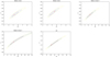 |
Fig. B.2. Best-fit statistics for the Lockman hole soft proton flare state spectra in E0 vs. b space. The chosen parameters are plotted as red crosses. Contours from inner to outer are 1σ, 2σ, and 3σ confidence levels. |
Best-fit parameters of flare state soft proton spectra in the Lockman Hole observation.
B.2. Vignetting function
The soft proton vignetting function is different from that of X-rays. To determine the spatial distribution of soft proton counts, we study the vignetting behaviour of different CCDs from the Lockman hole observation. We calculate surface brightness profiles with our surface brightness profile analysis tool. We take total count maps as the source images and quiescent state count maps as backgrounds. A uniform dummy exposure map is applied. The surface brightness profile of the residual soft protons reflects the vignetting behaviour.
The count weighted vignetting functions in the 2–10 keV band are shown in Fig. B.3. Because the MOS outer chips are closer to the mirror, there is a gap the vignetting functions of the central and outer CCDs. The vignetting behaviours of MOS1 and MOS2 centre CCDs are similar, but different in the outer CCDs. We fit vignetting functions with β profiles (Cavaliere & Fusco-Femiano 1976)
![$$ \begin{aligned} S(r) = S_0\left[1+\left(\frac{r}{r_0}\right)^2\right]^{0.5-3\beta }, \end{aligned} $$](/articles/aa/full_html/2020/10/aa37965-20/aa37965-20-eq16.gif)
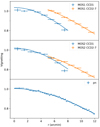 |
Fig. B.3. Vignetting functions of flare state soft protons detected by the EPIC CCDs in the 2–10 keV band determined from the Lockman hole observation. Each set of measurements is normalised to the second data point. Solid lines are best-fit β models. |
where r0 is fixed to 40′. Best fit parameters are listed in Table B.2.
Best fit parameters of 2–10 keV soft proton vignetting functions. Parameter r0 is fixed to 40′.
B.3. Self-calibration
We extract MOS and pn spectra from the Abell 3411 observation, separating the MOS centre and outer CCD region. We exclude the union of the MOS and pn bad pixel regions using additional region selection expressions. The selected regions are annuli centred at the pn focal point from 1′ to 12′ with width 1′. From the central MOS CCD region, we extract spectra up to r = 6′. From the outer MOS CCD region, we extract spectra from r = 8′. There are 3 × 5 centre region spectra and 3 × 4 outer region spectra in total. The energy range 0.5–14.0 keV is used for spectral fitting. Spectral components are the same as described in Table 2. We first fit FWC spectra with an exponential cut off power law and delta lines. We freeze the FWC continuum with the fitted cut-off power-law parameters and fit the soft proton and ICM components. We add two delta lines at 0.56 and 0.65 keV to fit the SWCX radiation. The other free parameters are Γ2 and L of soft proton components, norm, T and Z of the ICM. The best-fit values of a subset of the most relevant parameters are plotted in Fig. B.4.
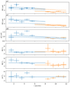 |
Fig. B.4. Radial profiles of L and Γ2 from the Abell 3411 observation. Blue points are from the centre MOS CCD region and orange points are from the outer MOS CCDs region. The best-fit radial models are plotted with lines. |
We use constant models to fit five Γ2 profiles, and use the vignetting models from Appendix B.2 to fit five luminosity profiles individually. We fix each β parameter but thaw the normalisation. Best-fit soft proton L0s and Γ2s are listed in the second and third columns of Table B.3, respectively. The best-fit model profiles are plotted with solid lines in Fig. B.4. If we assume the detector responses to SP are identical over time and in both flare and quiescent states, we can estimate the luminosity profiles in a second way. For this, we need to calculate the ratio of normalisations among different detectors. From Appendix B.2 we have surface brightness radial profiles at the flare state
Best-fit parameters and systematics of quiescent state soft proton components.
where  are the flare state spectrum models of different CCDs at radius r, and Vig is the vignetting function. Det can be MOS1 center, MOS1 outer, MOS2 center, MOS2 outer and pn. We take pn as a reference. The count rate ratio between other detectors and pn is
The energy flux ratio between other detectors and pn at the quiescent state can be easily calculated:
With the best-fit quiescent state Γ2, we obtain  s and list them in the fourth column of Table B.3. We couple the MOS L parameter to that of pn with the scale factor
  to fit the L profiles simultaneously. The best-fit L0 of pn is (9.5 ± 0.2)×1037W. We plot this set of luminosity models with dashed lines in Fig. B.4.
The systematic errors of radial luminosity models include two parts: one is the offset between the measured model (solid lines) and the empirical model on the basis of the Lockman Hole observation (dashed lines); another is from the intrinsic scatter that makes the χ2/d.o.f. of each profile in Fig. B.4 larger than 1.
The offset systematic errors, ηoff, are calculated using the formula  . The intrinsic systematic errors, ηin, are calculated such that
where  is the model luminosity at the ith point. The total systematic errors are then
  . We list the offset, intrinsic, and total systematic errors in the fifth to seventh columns of Table B.3.
We apply the self-calibrated soft proton model to spectra from regions of interest. Parameters E0 and b are fixed based on the values in Table B.1. Γ2 is fixed given in Table B.3. L is fixed to the value calculated from the vignetting function B.3 with β values from Table B.2 and normalisation values from the column L0 in B.3.
Appendix C: Cosmic X-ray background
Thanks to the Chandra observation, we are able to study the log N − log S relationship of point sources in the Abell 3411-3412 field. The result can help us to constrain the XMM-Newton point-source detection limit and to optimise point-source exclusion in the Suzaku analysis.
C.1. Point-source flux and the logN − logS relation
We use wavdetect to detect point sources in this field. An exposure-weighted PSF map is provided for source detection. The wavelet size is set as 1.0, 2.0, and 4.0. The task returns 147 sources in total. After visual inspection, 113 sources are left. We use roi to extract source and background regions for each point source. The background regions are set as elliptical annuli from 1.5 to 2.0 times the source radius. We extract spectra for each source from each observation using the task specextract. A point source aperture correction is applied. For each point source, all source and background spectra, as well as response files from each observation, are combined by combine_spectra. We model each point source spectrum with an absorbed power-law model. The energy range 0.5–7.0 keV is used for spectral fitting. We fit spectra with both a fixed Γ = 1.41 and a free Γ. If the relative error of Γ is less than 10%, we adopt the best-fit Γ and the corresponding flux. We exclude sources with zero fitted flux or Γ > 5 and compile the rest 101 sources into a catalogue.
To check the log N − log S relation of our sample, we plot the cumulative source number curve in Fig. C.1. The log N − log S relationship from the Chandra Deep Field South (CDF-S) has been well studied by Lehmer et al. (2012). X-ray point sources in the range 10−15 < S < 10−13 (erg s−1 cm−2) are dominated by AGNs (including X-ray binaries), and their distribution can be expressed by a broken power law,
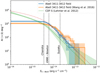 |
Fig. C.1. log N − log S curve from Chandra observations. The blue steps are from our analysis of the Abell 3411-3412 field. The best-fit power law is plotted as a blue dashed line. The model we assume to calculate the unresolved CXB in this field is shown as the red dotted line. The orange steps are from the Wang et al. (2016) catalogue of this field. As a comparison, the curve from CDF-S is plotted as a green line. The error of the CDF-S curve includes both Poisson error and the uncertainties on the best-fit parameters. The detection limits of Chandra and XMM-Newton as well as the Suzaku point-source exclusion limit in this paper are marked as vertical dotted lines. |
where Sref = 10−14 erg s−1 cm−2, and fb = 6.4 ± 1.0 × 10⁻¹⁵ erg s−1 cm−2 is the power-law break flux. The power-law index after the break flux is β2 = 2.55 ± 0.17. We plot the total CDF-S cumulative log N − log S curve in Fig. C.1 as well. The normalisation of the Abell 3411-3412 field is higher than that of the CDF-S. To cross check our point source flux analysis, we look up the catalogue compiled by Wang et al. (2016), which covers the Abell 3411-3412 field. In their work, for each source, the 0.3–8.0 keV flux is calculated with a fixed Γ = 1.7 and a free nH. We assume nH = 4.8 × 1020 cm−2 and convert the 0.3–8.0 keV flux to a 2–8 keV flux. The cumulative curve from that catalogue is also plotted. Though the methods of point-source flux calculation are different from our work, the log N − log S curve is consistent with ours at the faint end. At the bright end, the discrepancy is due to the assumptions for flux calculation. The consistency of results from two independent analyses proves that in this field, the number of point sources is much higher than the average value in the CDF-S. We fit our cumulative curve from 6 × 10⁻¹⁵ to 1 × 10⁻¹³ erg s−1 cm−2 using a single power-law model with a fixed cumulative index α = β2 + 1 = 1.55. The ratio between our normalisation to that from CDF-S is KA3411/KCDF − S = 2.03 ± 0.03.
C.2. Detection limit and CXB flux
From the cumulative log N − log S curve, the Chandra detection limit in this field is ∼3.5 × 10⁻¹⁵ erg s−1 cm−2. The detection limit of XMM-Newton is 6 × 10⁻¹⁵ erg s−1 cm−2; see Sect. 4.1 for details. The Suzaku detection limit is much higher because of the large PSF radius of rHEW = 1′. Excluding more point sources would make the spectrum fitting less biased by unresolved sources but would decrease the signal statistics at the same time. We exclude from the Suzaku analysis only point sources detected by Chandra with a flux above 2 × 10⁻¹⁴ s−1 cm−2. Point source coordinates are from the compiled Chandra catalogue. We inspect the chosen sources on the flux maps and additionally include two sources. One is a super-soft source (130.527°, −17.569°) whose photon index Γ = 3.8 causes the 2–8 keV flux F = 7.2 × 10⁻¹⁵ erg s−1 cm−2 to be below our exclusion limit. Another one is (130.561°, −17.657°), which is just at the edge of the Chandra field, but the source is bright in the XMM-Newton flux map. We shift all source coordinates to match the Suzaku astrometry.
The unresolved point source flux from CXBTools7 is based on the log N − log S relation from the work of Lehmer et al. (2012). As we have find the point source density in our field is twice higher than that of CDF-S, we need to take that into account to estimate the unresolved CXB level of XMM-Newton and Suzaku spectral components properly. The number density of point sources below the Chandra detection limit is unknown, but we speculate the dN/dS curve of our field will converge into the curve of CDF-S when S is small. We assume the convergent point is Scov = 1.4 × 10⁻¹⁶ erg s−1 cm−2, and at the breaking point of Lehmer et al. (2012)’s curve fb, the differential curve normalisation is twice that of the curve from CDF-S. We can express this relationship with the equation as below:
The solution of the function is α = 0.18. Therefore, in our field, the differential log N − log S relation is
and the unit of source flux is erg s−1 cm−2. The cumulative curve of this modified log N − log S model is plotted as the red dotted line in Fig. C.1.
We apply the differential log N − log S relation to estimate unresolved CXB flux in this paper. The unresolved CXB flux and its Poisson uncertainty can be expressed as
![$$ \begin{aligned}&F(S<S_\mathrm{lim} ) = A\left[F(S < S_\mathrm{cov} )+\int _{S_\mathrm{cov} }^{S_\mathrm{lim} }S\left(\frac{\mathrm{d} N}{\mathrm{d} S}\right)_\mathrm{A3411} \mathrm{d} S\right] \end{aligned} $$](/articles/aa/full_html/2020/10/aa37965-20/aa37965-20-eq31.gif)
where the unresolved flux below 1.4 × 10⁻¹⁶ erg s−1 cm−2 is 3.4 × 10⁻¹² erg s−1 cm−2 deg−2 (Hickox & Markevitch 2006), and A is the sky area of the selection region. The unresolved flux as a function of the detection limit is plotted in Fig. C.2 together with the relative error for a 1 deg2 sky area. For comparison, we over-plot the empirical relative error curve from Hoshino et al. (2010).
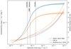 |
Fig. C.2. Unresolved CXB flux in the 2–8 keV band as a function of the point-source detection limit. The curves of CDF-S and our field are plotted with orange and blue lines, respectively. Dashed lines indicate the relative poisson error for 1 deg2 sky area. |
We note that for XMM-Newton data analysis, the actual CXB residual luminosity is not uniform due to the ICM emission. The detection limit extends to fainter point sources further out in radius as the ICM emission decreases. The point source sensitivity (in cgs units) can be expressed as
where  is the averaged photon energy, S the signal-to-noise ratio, A the effective area, t the exposure time, B the background counts per PSF beam, and P the PSF size. We use a quadratic function to model the radial increase of the PSF size and use a linear function to model the vignetting effect. The background B in the formula is composed of the cluster emission and other background components. The cluster emission is modelled by a β model (see Eq. (B.3)). The estimated 2D standard deviation of the residual CXB flux inside 10′ is ∼12%. As a comparison, based on the uncertainty curve in Fig. C.2, the CXB uncertainty contributed by the cosmic variance in a 3 arcmin2 selection region is ∼45% and this value will be larger in a smaller selection region. Therefore, we only take the cosmic variance into account. For Suzaku data analysis, we adopt the point-source exclusion limit based on the Chandra point-source catalogue, and can therefore assume a uniform residual CXB flux.
All Tables
Comparison of the southeast shock Mach number obtained from different instruments and methods.
Best-fit parameters of flare state soft proton spectra in the Lockman Hole observation.
Best fit parameters of 2–10 keV soft proton vignetting functions. Parameter r0 is fixed to 40′.
Best-fit parameters and systematics of quiescent state soft proton components.
All Figures
|
Fig. 1. Smoothed flux image of Abell 3411 combined from 1.2–4.0 keV XMM-Newton EPIC CCDs (left), 0.7–7.0 keV Suzaku XIS CCDs (middle), and 1.2–4.0 keV Chandra ACIS-I (right). Particle background and vignetting effect have been corrected. White contours are GMRT 610 MHz radio intensity. XMM-Newton and Suzaku analysis regions are plotted with cyan sectors. The locations of two BCGs are plotted with red crosses in the Chandra image. The coordinates of the BCGs are obtained from Golovich et al. (2019a). |
| In the text | |
|
Fig. 2. r500XMM-Newton-EPIC MOS1 (top left) and Suzaku XIS0 (top right) spectra as well as individual spectral components. We also plot residuals from the other two EPIC detectors (bottom left) and XIS detectors (bottom right). The fit statistics are C − stat/d.o.f = 1992/1554 for XMM-Newton EPIC spectra and C − stat/d.o.f = 563/423 for Suzaku XIS spectra. |
| In the text | |
|
Fig. 3. Temperature profiles of both Suzaku and XMM-Newton in the Suzaku SE selection region. Filled bands of each profile represent the major systematic errors, i.e. SP for XMM-Newton and CXB+GH for Suzaku. |
| In the text | |
|
Fig. 4. Surface brightness profile fitting results of SE, S, and cold front (CF) regions. Upper panel: Chandra surface brightness. Lower panel: XMM-Newton surface brightness profile fitted by fixed and free C parameters. All XMM-Newton models are smoothed by a σ = 0.1′ Gaussian function. Red lines indicate the ratio between the subtracted FWC background counts and the remaining signal, which include the ICM, X-ray background, and soft proton contamination. In regions where this ratio is higher than one, the FWC background dominates. Black dashed lines are the radio surface brightness profiles in an arbitrary unit. |
| In the text | |
|
Fig. 5. XMM-Newton temperature profile of each region. Dashed lines indicate edge locations fitted from surface brightness profiles. Grey bands indicate the temperature discrepancy between MOS and pn. |
| In the text | |
|
Fig. 6. Suzaku semicircle r500 selection region (red) and radial bins (green). |
| In the text | |
|
Fig. 7. Suzaku temperature profiles of the SE, S, and SW regions, as well as a comparison with the relaxed temperature profile in the outskirts predicted by numerical simulations. |
| In the text | |
|
Fig. 8. Suzaku flux map and the cyan spectral extraction regions are based on radio morphology (white contours). |
| In the text | |
|
Fig. 9. Suzaku and XMM-Newton temperature profiles from the radio-based selection regions in Fig. 8. The radio surface brightness profile is plotted as a black line. |
| In the text | |
|
Fig. 10. Shock Mach numbers derived from radio spectral index (ℳRadio) against those from the ICM temperature jump (ℳX). The data points of previous studies (grey) are adapted from Fig. 22 in van Weeren et al. (2019). The red point is the southwestern shock in Abell 3411-3412. |
| In the text | |
|
Fig. 11. XMM-Newton surface brightness profile of the northwest region. No density jump is found. |
| In the text | |
|
Fig. A.1. Inside FOV light curves for the three EPIC detectors in the 10–12 keV band with 100s bins. The filtered GTIs are shown as blue shadows. |
| In the text | |
|
Fig. A.2. Out-of-FOV 10–12 keV light curves of three EPIC detectors. Right panels: CDFs of count rates. For each light curve, the CDF of the Poisson distribution with μ from the data is plotted as a grey area. The p-values to reject the null hypothesis that the count rate distribution is Poissonian are labelled. |
| In the text | |
|
Fig. B.1. Flare state soft proton spectra in 12′ radius. |
| In the text | |
|
Fig. B.2. Best-fit statistics for the Lockman hole soft proton flare state spectra in E0 vs. b space. The chosen parameters are plotted as red crosses. Contours from inner to outer are 1σ, 2σ, and 3σ confidence levels. |
| In the text | |
|
Fig. B.3. Vignetting functions of flare state soft protons detected by the EPIC CCDs in the 2–10 keV band determined from the Lockman hole observation. Each set of measurements is normalised to the second data point. Solid lines are best-fit β models. |
| In the text | |
|
Fig. B.4. Radial profiles of L and Γ2 from the Abell 3411 observation. Blue points are from the centre MOS CCD region and orange points are from the outer MOS CCDs region. The best-fit radial models are plotted with lines. |
| In the text | |
|
Fig. C.1. log N − log S curve from Chandra observations. The blue steps are from our analysis of the Abell 3411-3412 field. The best-fit power law is plotted as a blue dashed line. The model we assume to calculate the unresolved CXB in this field is shown as the red dotted line. The orange steps are from the Wang et al. (2016) catalogue of this field. As a comparison, the curve from CDF-S is plotted as a green line. The error of the CDF-S curve includes both Poisson error and the uncertainties on the best-fit parameters. The detection limits of Chandra and XMM-Newton as well as the Suzaku point-source exclusion limit in this paper are marked as vertical dotted lines. |
| In the text | |
|
Fig. C.2. Unresolved CXB flux in the 2–8 keV band as a function of the point-source detection limit. The curves of CDF-S and our field are plotted with orange and blue lines, respectively. Dashed lines indicate the relative poisson error for 1 deg2 sky area. |
| In the text | |
Current usage metrics show cumulative count of Article Views (full-text article views including HTML views, PDF and ePub downloads, according to the available data) and Abstracts Views on Vision4Press platform.
Data correspond to usage on the plateform after 2015. The current usage metrics is available 48-96 hours after online publication and is updated daily on week days.
Initial download of the metrics may take a while.