© ESO, 2017

1. Introduction

An intense focus in current observational cosmology is detection of the cosmic microwave background (CMB) B-mode signal induced by primordial gravitational waves during the inflation era (Starobinsky 1979; Fabbri & Pollock 1983; Abbott & Wise 1984). The BICEP2 experiment¹ puts an upper bound on the amplitude of the CMB B-mode signal, parameterized by a tensor-to-scalar ratio (r) at a level of r< 0.09 (95% confidence level BICEP2 and Keck Array Collaboration et al. 2016). Therefore, the major challenge for a BICEP2-like experiment with limited frequency coverage is to detect such an incredibly faint CMB B-mode signal in the presence of foreground Galactic contamination (Betoule et al. 2009). The dominant polarized foreground above 100GHz come from thermal emission by aligned aspherical dust grains (Planck Collaboration Int. XXII 2015; Planck Collaboration X 2016). Unlike the CMB, the polarized dust emission is distributed non-uniformly on the sky with varying column density over which are summed contributions from multiple components with different dust composition, size, and shape and with different magnetic field orientation (see reviews by Prunet & Lazarian 1999; Lazarian 2008). Acknowledging these complexities, the goal of this paper is to model the principal effects, namely multiple components with different magnetic field orientations, to produce realistic simulated maps of the polarized dust emission.

Our knowledge and understanding of the dust polarization has improved significantly in the submillimetre and microwave range through exploitation of data from the Planck satellite² (Planck Collaboration I 2016; Planck Collaboration X 2016; Planck Collaboration Int. XIX 2015), which provides important empirical constraints on the models. The Planck satellite has mapped the polarized sky at seven frequencies between 30 and 353GHz (Planck Collaboration I 2016). The Planck maps are available in HEALPix³ format (Górski et al. 2005) with resolution parameter labelled with the N_side value. The general statistical properties of the dust polarization in terms of angular power spectrum at intermediate and high Galactic latitudes from 100 to 353GHz are quantified in Planck Collaboration Int. XXX (2016).

Two unexpected results from the Planck observations were an asymmetry in the amplitudes of the angular power spectra of the dust E- and B-modes (EE and BB spectra, respectively) and a positive temperature E-mode (TE) correlation at 353GHz. Explanation of these important features was explored by Planck Collaboration Int. XXXVIII (2016) through a statistical study of the filamentary structures in the Planck Stokesmaps and Caldwell et al. (2017) discussed them in the context of magnetohydrodynamic interstellar turbulence. They are a central focus of the modelling in this paper.

The Planck 353GHz polarization maps (Planck Collaboration Int.XIX 2015) have the best signal-to-noise ratio and enable study of the link between the structure of the Galactic magnetic field (GMF) and dust polarization properties. A large scatter of the dust polarization fraction (p) for total column density N_H< 10²² cm^-2 at low and intermediate Galactic latitudes is reported in Planck Collaboration Int. XIX (2015). Based on numerical simulations of anisotropic magnetohydrodynamic turbulence in the diffuse interstellar medium (ISM), it has been concluded that the large scatter of p in the range 2 × 10²¹ cm^-2<N_H< 2 × 10²² cm^-2 comes mostly from fluctuations in the GMF orientation along the line of sight (LOS) rather than from changes in grain shape or the efficiency of the grain alignment (Planck Collaboration Int. XX 2015). To account for the observed scatter of p in the high latitude southern Galactic sky (b ≤ −60°), a finite number of polarization layers was introduced (Planck Collaboration Int. XLIV 2016). The orientation of large-scale GMF with respect to the plane of the sky (POS) also plays a crucial role in explaining the scatter of p (Planck Collaboration Int. XX 2015).

The Planck polarization data reveal a tight relationship between the orientation of the dust intensity structures and the magnetic field projected on the plane of the sky (B_POS, Planck Collaboration Int. XXXII 2016; Planck Collaboration Int.XXXV 2016; Planck Collaboration Int.XXXVIII 2016). In particular, the dust intensity structures are preferentially aligned with B_POS in the diffuse ISM (Planck Collaboration Int. XXXII 2016). Similar alignment is also reported between the Galactic Arecibo L-Band Feed Array (GALFA, Peek et al. 2011) HI filaments and B_POS derived either from starlight polarization (Clark et al. 2014) or Planck polarization data (Clark et al. 2015). Furthermore, a detailed all-sky study of the HI filaments, combining the Galactic All Sky Survey (GASS, McClure-Griffiths et al. 2009) and the Effelsberg Bonn HI Survey (EBHIS, Winkel et al. 2016), shows that most of the filaments occur in the cold neutral medium (CNM, Kalberla et al. 2016). The HI emission in the CNM phase has a line profile with 1σ velocity dispersion 3kms^-1 (FWHM 7kms^-1) in the solar neighbourhood (Heiles & Troland 2003) and filamentary structure on the sky, which might result from projection effects of gas organized primarily in sheets (Heiles & Troland 2005; Kalberla et al. 2016). Alignment of CNM structures with B_POS from Planck has been reported towards the north ecliptic pole, among the targeted fields of the Green Bank Telescope HI Intermediate Galactic Latitude Survey (GHIGLS, Martin et al. 2015). Such alignment can be induced by shear strain of gas turbulent velocities stretching matter and the magnetic field in the same direction (Hennebelle 2013; Inoue & Inutsuka 2016).

Alignment between the CNM structures and B_POS was not included in the pre-Planck dust models, for example Planck Sky Model (PSM, Delabrouille et al. 2013) and FGPol (O’Dea et al. 2012). The most recent version of post-Planck PSM uses a filtered version of the Planck 353GHz polarization data as the dust templates (Planck Collaboration XII 2016). Therefore, in low signal-to-noise regions the PSM dust templates are not reliable representations of the true dust polarized sky. In Planck Collaboration Int. XXXVIII (2016) it was shown that preferential alignment of the dust filaments with B_POS could account for both the E-B asymmetry in the amplitudes of the dust ${\mathrm{𝒟}}_{\mathit{\ell }}^{\mathit{EE}}$ and ${\mathrm{𝒟}}_{\mathit{\ell }}^{\mathit{BB}}$ angular power spectra⁴ over the multipole range 40 <ℓ< 600 and the amplitude ratio ${\mathrm{𝒟}}_{\mathit{\ell }}^{\mathit{TE}}$/${\mathrm{𝒟}}_{\mathit{\ell }}^{\mathit{EE}}$, as measured by Planck Collaboration Int. XXX (2016). Clark et al. (2015) showed that the alignment of the B_POS with the HI structures can explain the observed E-B asymmetry.

Recently, Vansyngel et al. (2017) have extended the approach introduced in Planck Collaboration Int. XLIV (2016) using a parametric model to account for the observed dust power spectra at intermediate and high Galactic latitudes. Our work in this paper is complementary, incorporating additional astrophysical data and insight and focusing on the cleanest sky area for CMB B-mode studies from the southern hemisphere.

In more detail, the goal of this paper is to test whether preferential alignment of the CNM structures with B_POS together with fluctuations in the GMF orientation along the LOS can account fully for a number of observed statistical properties of the dust polarization over the southern low column density sky. These statistical properties include the scatter of the polarization fraction p, the dispersion of the polarization angle ψ around the large-scale GMF, and the observed dust power spectra ${\mathrm{𝒟}}_{\mathit{\ell }}^{\mathit{EE}}$, ${\mathrm{𝒟}}_{\mathit{\ell }}^{\mathit{BB}}$, and ${\mathrm{𝒟}}_{\mathit{\ell }}^{\mathit{TE}}$ at 353GHz. In doing so we extend the analysis of Planck Collaboration Int. XXXVIII (2016) and Planck Collaboration Int. XLIV (2016) to sky areas in which the filaments have very little contrast with respect to the diffuse background emission. Within the southern Galactic cap (defined here to be b ≤ −30°), in which dust and gas are well correlated (Boulanger et al. 1996; Planck Collaboration XI 2014) and the GASS HI emission is a good tracer of the dust intensity structures (Planck Collaboration Int. XVII 2014),we focus our study on the low column density portion. We choose to model the dust polarization sky at 1° resolution, which corresponds to retaining multipoles ℓ ≤ 160 where the Galactic dust dominates over the CMB B-mode signal. Also, most of the ground-based CMB experiments are focusing at a degree scale for the detection of the recombination bump of the CMB B-mode signal. Our dust polarization model should be a useful product for the CMB community. It covers 34% of the southern Galactic cap, a 3500 deg² region containing the cleanest sky accessible to ongoing ground and balloon-based CMB experiments: ABS (Essinger-Hileman et al. 2010), Advanced ACTPol (Henderson et al. 2016), BICEP/ Keck (Ogburn et al. 2012), CLASS (Essinger-Hileman et al. 2014), EBEX (Reichborn-Kjennerud et al. 2010), Polarbear (Kermish et al. 2012), Simons array (Suzuki et al. 2016), SPIDER (Crill et al. 2008), and SPT3G (Benson et al. 2014).

This paper is organized as follows. Section2 introduces the Planck observations and GASS H I data used in our analysis, along with a selected sky region within the southern Galactic cap, called SGC34. In Sect.3, we summarize the observational dust polarization properties in SGC34 as seen by Planck. A model to simulate dust polarization using the GASS HI data and a phenomenological description of the GMF is detailed in Sect.4. The procedure to simulate the polarized dust sky towards the southern Galactic cap and the choice of the dust model parameters are discussed in Sect.5. Section5.4 presents the main results where we statistically compare the dust model with the observed Planck data. In Sect.6, we make some predictions using our dust model. We end with an astrophysical perspective in Sect.7 and a short discussion and summary of our results in Sect.8.

2. Data sets used and region selection

2.1. Planck 353GHz data

In this paper we used the publicly available⁵ maps from the Planck 2015 polarization data release (PR2), specifically at 353GHz (Planck Collaboration I 2016)⁶. The data processing and calibration of the Planck High Frequency Instrument (HFI) maps are described in Planck Collaboration VIII (2016). We used multiple Planck 353GHz polarization data sets: the two yearly surveys, Year 1 (Y1) and Year 2 (Y2), the two half-mission maps, HM1 and HM2, and the two detector-set maps, DS1 and DS2, to exploit the statistical independence of the noise between them and to test for any systematic effects⁷. The 353GHz polarization maps are corrected for zodiacal light emission at the map-making level (Planck Collaboration VIII 2016). These data sets are described in full detail in Planck Collaboration VIII (2016).

All of the 353GHz data sets used in this study have an angular resolution of FWHM 4.′82 and are projected on a HEALPix grid with a resolution parameter N_side=2048 (1.′875pixels). We corrected for the main systematic effect, that is leakage from intensity to polarization, using the global template fit, as described in Planck Collaboration VIII (2016), which accounts for the monopole, calibration, and bandpass mismatches. To increase the signal-to-noise ratio of the Planck polarization measurements over SGC34, we smoothed the Planck polarization maps to 1° resolution using a Gaussian approximation to the Planck beam and reprojected to a HEALPix grid with N_side=128(30′pixels). We did not attempt to correct for the CMB polarization anisotropies at 1° resolution because they are negligibly small compared to the dust polarization at 353GHz.

The dust intensity at 353GHz, D₃₅₃, is calculated from the latest publicly available Planck thermal dust emission model (Planck Collaboration Int. XLVIII 2016), which is a modified blackbody (MBB) fit to maps at ν ≥ 353GHz from which the cosmic infrared background anisotropies (CIBA) have been removed using the generalized linear internal combination (GNILC) method and zero-level offsets (e.g. the CIB monopole) have been removed by correlation with H I maps at high Galactic latitude. By construction, this dust intensity map is corrected for zodiacal light emission, CMB anisotropies, and resolved point sources as well as the CIBA and the CIB monopole. As a result of the GNILC method and the MBB fitting, the noise in the D₃₅₃ map is lower than in the StokesI frequency map at 353GHz. We also smoothed the D₃₅₃ map to the common resolution of 1°, taking into account the effective beam resolution of the map.

2.2. GASS Hi data

We use the GASS H I survey⁸ (McClure-Griffiths et al. 2009; Kalberla et al. 2010; Kalberla & Haud 2015) which mapped the southern sky (declination δ< 1°) with the Parkes telescope at an angular resolution of FWHM 14.′4. The rms uncertainties of the brightness temperatures per channel are at a level of 57mK at δv = 1kms^-1. The GASS survey is the most sensitive and highest angular resolution survey of H I emission over the southern sky. The third data release version has improved performance by the removal of residual instrumental problems along with stray radiation and radio-frequency interference, which can be major sources of error in H I column density maps (Kalberla & Haud 2015). The GASS HI data are projected on a HEALPix grid with N_side=1024 (3.′75pixels).

For this optically thin gas, the brightness temperature spectra T_b of the GASS H I data are decomposed into multiple Gaussian components (Haud & Kalberla 2007; Haud 2013) as ${\mathit{T}}_{\mathrm{b}}\mathrm{=}\sum _{\mathit{i}}{\mathit{T}}_{\mathrm{0}}^{\mathit{i}}\exp \left[\mathrm{-}\frac{\mathrm{1}}{\mathrm{2}}{\left(\frac{{\mathit{v}}_{\mathrm{LSR}}\mathrm{-}{\mathit{v}}_{\mathrm{c}}^{\mathit{i}}}{{\mathit{\sigma }}^{\mathit{i}}}\right)}^{\mathrm{2}}\right]\mathit{,}$(1)where the sum is over all Gaussian components for a LOS, v_LSR is the velocity of the gas relative to the local standard of rest (LSR), and ${\mathit{T}}_{\mathrm{0}}^{\mathit{i}}$, ${\mathit{v}}_{\mathrm{c}}^{\mathit{i}}$, and σⁱ are the peak brightness temperature (inK), central velocity, and 1σ velocity dispersion of the ith Gaussian component, respectively. Although the Gaussian decomposition does not provide a unique solution, it is correct empirically. Haud (2013) used the GASS survey at N_side=1024 and decomposed the observed 6655155 HI profiles into 60349584Gaussians. In this study, we use an updated (but unpublished) Gaussian decomposition of the latest version of the GASS HI survey (third data release). The intermediate and high velocity gas over the southern Galactic cap has negligible dust emission (see discussion in Planck Collaboration Int. XVII 2014) and in any case lines of sight with uncorrelated dust and H I emissions are removed in our masking process (Sect.2.3).

Broadly speaking, the Gaussian H I components represent the three conventional phases of the ISM. In order of increasing velocity dispersion these are: (1) a cold dense phase, the CNM, with a temperature in the range ~40−200K; (2) a thermally unstable neutral medium (UNM), with a temperature in the range ~200−5000K; and (3) a warm diffuse phase, the warm neutral medium (WNM), with a temperature in the range ~5000−8000K. Based on sensitive high-resolution Arecibo observations, Heiles & Troland (2003) found that a significant fraction of the H I emission is in the UNM phase at high Galactic latitude. Numerical simulations of the ISM suggest that the magnetic field and dynamical processes like turbulence could drive H I from the stable WNM and CNM phases into the UNM phase (Audit & Hennebelle 2005; Hennebelle & Iffrig 2014; Saury et al. 2014).

The total H I column density along the LOS, N_Hi, in units of 10¹⁸ cm^-2, is obtained by integrating the brightness temperature over velocity. We can separate the total N_Hi into the three different phases of the ISM based on the velocity dispersion of the fitted Gaussian. Thus $\begin{array}{ccc}{\mathit{N}}_{\mathrm{H}\hspace{0.17em}{i}}& \mathrm{=}& \mathrm{1.82}\mathrm{\times }\mathrm{\int }{\mathit{T}}_{\mathrm{b}}\mathrm{d}{\mathit{v}}_{\mathrm{LSR}}\\ & \mathrm{=}& \mathrm{1.82}\mathrm{\times }\mathrm{\int }\sum _{\mathit{i}}{\mathit{T}}_{\mathrm{0}}^{\mathit{i}}\exp \left[\mathrm{-}\frac{\mathrm{1}}{\mathrm{2}}{\left(\frac{{\mathit{v}}_{\mathrm{LSR}}\mathrm{-}{\mathit{v}}_{\mathrm{c}}^{\mathit{i}}}{{\mathit{\sigma }}^{\mathit{i}}}\right)}^{\mathrm{2}}\right]\mathrm{d}{\mathit{v}}_{\mathrm{LSR}}\\ & \mathrm{=}& \mathrm{1.82}\mathrm{\times }\sqrt{\mathrm{2}\mathit{\pi }}\begin{array}{c}\sum \end{array}\mathrm{(}{\mathit{T}}_{\mathrm{0}}^{\mathit{i}}{\mathit{\sigma }}^{\mathit{i}}{\mathit{w}}_{\mathrm{c}}\mathrm{+}{\mathit{T}}_{\mathrm{0}}^{\mathit{i}}{\mathit{\sigma }}^{\mathit{i}}{\mathit{w}}_{\mathrm{u}}\mathrm{+}{\mathit{T}}_{\mathrm{0}}^{\mathit{i}}{\mathit{\sigma }}^{\mathit{i}}{\mathit{w}}_{\mathrm{w}}\mathrm{)}\\ & \mathrm{\equiv }& \end{array}$(2)where w_c, w_u, and w_w are the weighting factors to select the CNM, UNM, and WNM components, respectively, and ${\mathit{N}}_{{Hi}}^{\mathrm{c}}$, ${\mathit{N}}_{{Hi}}^{\mathrm{u}}$, and ${\mathit{N}}_{{Hi}}^{\mathrm{w}}$ are the CNM, UNM, and WNM column densities, respectively. The weighting factors are defined as $\begin{array}{ccc}& & {\mathit{w}}_{\mathrm{c}}\mathrm{=}\{\begin{array}{c}\\ & \\ & \\ & \end{array}\\ & & {\mathit{w}}_{\mathrm{w}}\mathrm{=}\{\begin{array}{c}\\ & \\ & \\ & \end{array}\\ & & {\mathit{w}}_{\mathrm{u}}\mathrm{=}\mathrm{1}\mathrm{-}{\mathit{w}}_{\mathrm{c}}\mathrm{-}{\mathit{w}}_{\mathrm{w}}\mathit{.}\end{array}$(3)We use overlapping weighting factors to avoid abrupt changes in the assignment of the emission from a given H I phase to another, adopting g = 0.2. There is a partial correlation between two neighbouring H I components. To select local velocity gas, we included only Gaussian components with $\mathrm{\left|}{\mathit{v}}_{\mathrm{c}}^{\mathit{i}}\mathrm{\right|}\mathrm{\le }\mathrm{50}\mathrm{km}{\mathrm{s}}^{-1}$.

For our analysis we also smoothed these N_Hi maps to the common resolution of 1°, taking into account the effective beam resolution of the map. Figure1 shows the separation of the total N_Hi into the three Gaussian-based H I phases, CNM, UNM, and WNM. The weights were calculated with σ_c = 7.5 km s^-1 and σ_u = 10 km s^-1 as adopted in Sect.5.2. The total N_Hi map obtained by summing these component phases is very close to the Low velocity cloud (LVC) map in Fig.1 of Planck Collaboration Int. XVII (2014) obtained by integrating over the velocity range defined by Galactic rotation, with dispersion only 0.012 × 10²⁰cm^-2 in the difference or 0.8% in the fractional difference over the selected region SGC34 defined below.

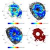Fig. 1 NHi maps of the three Gaussian-based HI phases: CNM (top left), UNM (top right), and WNM (bottom left) over the portion of the southern Galactic cap (b ≤ −30°) covered by the GASS HI survey, at 1° resolution. Coloured region corresponds to the selected region SGC34 (bottom right). Orthographic projection in Galactic coordinates: latitudes and longitudes marked by lines and circles respectively.

To build our CNM map we use an upper limit to the velocity dispersion (σ_c = 7.5 km s^-1) larger than the conventional line width of cold H I gas (Wolfire et al. 2003; Heiles & Troland 2005; Kalberla et al. 2016). The line width can be characterised by a Doppler temperature T_D. Because the line width includes a contribution from turbulence, T_D is an upper limit to the gas kinetic temperature. In Kalberla et al. (2016), the median Doppler temperature of CNM gas is about T_D = 220K, corresponding to a velocity dispersion of about σ_c = 1.3kms^-1, while the largest value of T_D = 1100K corresponds to σ_c = 3.0kms^-1. The value of σ_c = 7.5kms^-1 in our model follows from the model fit to the Planck polarization data (the observed E−B asymmetry and the ${\mathrm{𝒟}}_{\mathit{\ell }}^{\mathit{TE}}$/${\mathrm{𝒟}}_{\mathit{\ell }}^{\mathit{EE}}$ ratio over SGC34, see Sect.5.2). Thus our CNM component (${\mathit{N}}_{{Hi}}^{\mathrm{c}}$) includes some UNM gas. To investigate the impact of this on our modelling, we divided our CNM component map into two parts corresponding to components with velocity dispersions above and below σ_c = 3.0 km s^-1. We then repeated our data fitting with these two separate maps replacing our single CNM component map and found no significant difference in the model results.

2.3. Selection of the region SGC34

For our analysis we select a low dust column density region of the sky within the southern Galactic cap. As a first cut, we retain only the sky pixels that have N_Hi below a threshold value, N_{H i} ≤ 2.7 × 10²⁰ cm^-2. Molecular gas is known from UV observations to be negligible at this threshold N_Hi value (Gillmon et al. 2006). We adopt a second mask, from Planck Collaboration Int. XVII (2014), to avoid sky pixels that fall off the main trend of gas-dust correlation between the GASS H I column density and Planck HFI intensity maps, in particular applying a threshold of 0.21MJysr^-1 (3σ cut, see Fig.4 of Planck Collaboration Int. XVII 2014) on the absolute value of the residual emission at 857GHz after subtraction of the dust emission associated with HI gas. We smooth the second mask to Gaussian 1° FWHM resolution and downgrade to N_side=128 HEALPix resolution. Within this sky area, we also mask out a 10° radius patch centred around to avoid H I emission from the Magellanic stream, whose mean radial velocity for this specific sky patch is within the Galactic range of velocities (Nidever et al. 2010).

After masking, we are left with a 3500 deg² region comprising 34% of the southern Galactic cap, referred to hereafter as SGC34. This is presented in Fig.1. The mean N_Hi over SGC34 is ⟨ N_Hi ⟩ = 1.58 × 10²⁰cm^-2. For the adopted values of σ_c and σ_u, the mean column densities of the three ISM phases (Fig.1) are $\mathrm{⟨}{\mathit{N}}_{{Hi}}^{\mathrm{c}}\mathrm{⟩}\mathrm{=}\mathrm{0.66}\mathrm{\times }{\mathrm{10}}^{\mathrm{20}}\mathrm{c}{\mathrm{m}}^{-2}$, $\mathrm{⟨}{\mathit{N}}_{{Hi}}^{\mathrm{u}}\mathrm{⟩}\mathrm{=}\mathrm{0.49}\mathrm{\times }{\mathrm{10}}^{\mathrm{20}}\mathrm{c}{\mathrm{m}}^{-2}$, and $\mathrm{⟨}{\mathit{N}}_{{Hi}}^{\mathrm{w}}\mathrm{⟩}\mathrm{=}\mathrm{0.43}\mathrm{\times }{\mathrm{10}}^{\mathrm{20}}\mathrm{c}{\mathrm{m}}^{-2}$. SGC34 has a mean dust intensity of ⟨ D₃₅₃ ⟩ = 54 kJysr^-1. Correlating the total N_Hi map with the D₃₅₃ map, we find an emissivity (slope) 32 kJysr^-1(10²⁰ cm^-2)^-1 at 353GHz (Sect.5.2) and an offset of just 3kJysr^-1, which we use below as a 1σ uncertainty on the zero-level of the Galactic dust emission.

For computations of the angular power spectrum, we apodized the selection mask by convolving it with a 2° FWHM Gaussian. The effective sky coverage of SGC34 as defined by the mean sky coverage of the apodized mask is ${\mathit{f}}_{\mathrm{sky}}^{\mathrm{eff}}\mathrm{=}\mathrm{0.085}$ (8.5%), meaning that the smoothing extends the sky region slightly but conserves the effective sky area.

2.4. Power spectrum estimator

We use the publicly available Xpol code (Tristram et al. 2005) to compute the binned angular power spectra over a given mask. A top-hat binning in intervals of 20 ℓ over the range 40 <ℓ< 160 is applied throughout this analysis. The upper cutoff ℓ_max = 160 is set by 1° smoothed maps used throughout this paper. The lower cutoff ℓ_min = 40 is chosen to avoid low ℓ systematic effects present in the publicly available Planck polarization data (Planck Collaboration Int. XLVI 2016). The Xpol code corrects for the incomplete sky coverage, leakage from E- to B-mode polarization, beam smoothing, and pixel window function. Other codes such as PolSpice (Chon et al. 2004) and Xpure (Grain et al. 2009) also compute angular power spectra from incomplete sky coverage. We prefer Xpol over other codes because it directly computes the analytical error bars of the power spectrum without involving any Monte-Carlo simulations. The final results of this paper do not depend on the Xpol code, as the same mean power spectra are returned by other power spectrum estimators.

3. Planck dust polarization observations over the selected region SGC34

In this section we derive the statistical properties of the Planck dust polarization over SGC34. These statistical properties include normalized histograms from pixel space data, specifically of p² and of ψ with respect to the local polarization angle of the large-scale GMF, and the polarized dust power spectra in the harmonic domain.

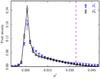Fig. 2 Normalized histograms of p2 over SGC34 at 353GHz. Planck data, ${\mathit{p}}_{\mathrm{d}}^{\mathrm{2}}$, blue inverted-triangles, with 1σerror bars as described in text. The pixel density on the y-axis is the number of pixels in each bin of p2 divided by the total number of pixels over SGC34. Dust model, ${\mathit{p}}_{\mathrm{m}}^{\mathrm{2}}$, black circles connected by line, with 1σ error bars computed from 100Monte-Carlo realizations. The vertical dashed line corresponds to the parameter p0 = 18.5% (${\mathit{p}}_{\mathrm{0}}^{\mathrm{2}}\mathrm{=}\mathrm{0.034}$) of this dust model.

3.1. Polarization fraction

The naive estimator of p, defined as $\mathit{p}\mathrm{=}\sqrt{{\mathit{Q}}^{\mathrm{2}}\mathrm{+}{\mathit{U}}^{\mathrm{2}}}\mathit{/}\mathit{I}$, is a biased quantity. The bias in p becomes dominant in the low signal-to-noise regime (Simmons & Stewart 1985). Montier et al. (2015) review the different algorithms to debias the p estimate. To avoid the debiasing problem, we choose to work with the unbiased quantity ${\mathit{p}}_{\mathrm{d}}^{\mathrm{2}}$ derived from a combination of independent subsets of the Planck data at 353GHz (see Eq.(12) of Planck Collaboration Int. XLIV 2016): 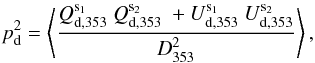${\mathit{p}}_{\mathrm{d}}^{\mathrm{2}}\mathrm{=}⟨\frac{{\mathit{Q}}_{\mathrm{d}\mathit{,}\mathrm{353}}^{{\mathrm{s}}_{\mathrm{1}}}{\mathit{Q}}_{\mathrm{d}\mathit{,}\mathrm{353}}^{{\mathrm{s}}_{\mathrm{2}}}\mathrm{+}{\mathit{U}}_{\mathrm{d}\mathit{,}\mathrm{353}}^{{\mathrm{s}}_{\mathrm{1}}}{\mathit{U}}_{\mathrm{d}\mathit{,}\mathrm{353}}^{{\mathrm{s}}_{\mathrm{2}}}}{{\mathit{D}}_{\mathrm{353}}^{\mathrm{2}}}⟩\mathit{,}$(4)where the subscript “d” refers to the observed polarized dust emission from the Planck 353GHz data (as distinct from “m” for the model below).

Normalized histograms of ${\mathit{p}}_{\mathrm{d}}^{\mathrm{2}}$ are computed over SGC34 from the cross-products of the three subsets of the Planck data where (s₁,s₂)={(HM1, HM2), (Y1,Y2), (DS1, DS2)}. Figure2 presents the mean of these three normalized histograms (blue inverted-triangles). The two main sources of uncertainty that bias the normalized histogram of ${\mathit{p}}_{\mathrm{d}}^{\mathrm{2}}$ are data systematics and the uncertainty of the zero-level of the Galactic dust emission. The former is computed per histogram bin using the standard deviation of ${\mathit{p}}_{\mathrm{d}}^{\mathrm{2}}$ from the three subsets of the Planck data. The latter is propagated by changing the dust intensity D₃₅₃ by ±3kJysr^-1. The total 1σ error bar per histogram bin is the quadrature sum of these two uncertainties.

The mean, median, and maximum values of the dust polarization fraction for the three subsets of the Planck data are presented in Table1. The maximum value of p_d at 1° resolution is consistent with the ones reported in Planck Collaboration Int.XLIV (2016) over the high latitude southern Galactic cap and the Planck Collaboration Int. XIX (2015) value at low and intermediate Galactic latitudes. We define a sky fraction f(p_d> 25%) where the observed dust polarization fraction is larger than a given value of 25% or ${\mathit{p}}_{\mathrm{d}}^{\mathrm{2}}\mathit{>}\mathrm{0.0625}$. In SGC34 this fraction is about 1%. The small scatter between the results from the three different subsets shows that the Planck measurements are robust against any systematic effects.

The negative values of ${\mathit{p}}_{\mathrm{d}}^{\mathrm{2}}$ computed from Eq.(4) arise from instrumental noise present in the three subsets of the Planck data. The width of the ${\mathit{p}}_{\mathrm{d}}^{\mathrm{2}}$ normalized histogram is narrower than the width reported by Planck Collaboration Int. XLIV (2016) over the high latitude southern Galactic cap. We were able to reproduce the broader distribution of ${\mathit{p}}_{\mathrm{d}}^{\mathrm{2}}$ by adopting the same analysis region as in Planck Collaboration Int. XLIV (2016), showing the sensitivity to the choice of sky region.

3.2. Polarization angle

We use multiple subsets of the Planck polarization data at 353GHz to compute the normalized Stokesparameters ${\mathit{q}}_{\mathrm{d}\mathit{,}\mathrm{353}}^{\mathrm{s}}\mathrm{=}{\mathit{Q}}_{\mathrm{d}\mathit{,}\mathrm{353}}^{\mathrm{s}}\mathit{/}{\mathit{D}}_{\mathrm{353}}$ and ${\mathit{u}}_{\mathrm{d}\mathit{,}\mathrm{353}}^{\mathrm{s}}\mathrm{=}{\mathit{U}}_{\mathrm{d}\mathit{,}\mathrm{353}}^{\mathrm{s}}\mathit{/}{\mathit{D}}_{\mathrm{353}}$, where s = {DS1, DS2, HM1, HM2, Y1, Y2}. Using these data over SGC34, we fit the mean direction of the large-scale GMF, as defined by two coordinates l₀ and b₀, using model A of Planck Collaboration Int.XLIV (2016). The best-fit values of l₀ and b₀ for each of the six independent subsets of the Planck data are quoted in Table1. The mean values of l₀ and b₀ and their dispersions from the independent subsets are and , respectively. Our error bars are smaller than those (5°) reported by Planck Collaboration Int. XLIV (2016) because the latter include the difference between fit values obtained with and without applying the bandpass mismatch (BPM) correction described in Sect. A.3 of Planck Collaboration VIII (2016). The mean values of l₀ and b₀ reported by Planck Collaboration Int. XLIV (2016) were derived using maps with no correction applied. The difference of relative to our mean value of l₀ arises primarily from the BPM correction used in our analysis.

Fig. 3 Similar to Fig.2, but for normalized histograms of ψR, the polarization angle relative to the local polarization angle of the large-scale GMF. The vertical dashed line corresponds to a model in which the turbulence is absent (Bturb = 0 so that ψR = 0°).

The best-fit values of l₀ and b₀ are used to derive a map of a mean-field polarization angle ${\mathit{\psi }}_{\mathrm{0}}\mathrm{\left(}\hat{{n}}\mathrm{\right)}$ (see Planck Collaboration Int. XLIV 2016, for the Q and U patterns associated with the mean field). We then rotate each sky pixel with respect to the new reference angle ${\mathit{\psi }}_{\mathrm{0}}\mathrm{\left(}\hat{{n}}\mathrm{\right)}$, using the relation $\begin{array}{ccc}\left[\begin{array}{c}\\ \\ \end{array}\right]& \mathrm{=}& \left(\begin{array}{c}\\ & & \\ & & \end{array}\right)\\ & & \mathrm{\times }\left[\begin{array}{c}\\ \\ \end{array}\right]\mathit{,}\end{array}$(5)where ${\mathit{Q}}_{\mathrm{d}\mathit{,}\mathrm{353}}^{\mathrm{R}}$ and ${\mathit{U}}_{\mathrm{d}\mathit{,}\mathrm{353}}^{\mathrm{R}}$ are the new rotated Stokesparameters. The “butterfly patterns” caused by the large-scale GMF towards the southern Galactic cap (Planck Collaboration Int. XLIV 2016) are now removed from the dust polarization maps. Non-zero values of the polarization angle, ${\mathit{\psi }}_{\mathrm{d}}^{\mathrm{R}}$, derived from the ${\mathit{Q}}_{\mathrm{d}\mathit{,}\mathrm{353}}^{\mathrm{R}}$ and ${\mathit{U}}_{\mathrm{d}\mathit{,}\mathrm{353}}^{\mathrm{R}}$ maps via ${\mathit{\psi }}_{\mathrm{d}}^{\mathrm{R}}\mathrm{\left(}\hat{{n}}\mathrm{\right)}\mathrm{=}\frac{\mathrm{1}}{\mathrm{2}}{\tan }^{-1}\mathrm{(}\mathrm{-}{\mathit{U}}_{\mathrm{d}\mathit{,}\mathrm{353}}^{\mathrm{R}}\mathrm{(}\hat{{n}}\mathrm{)}\mathit{,}{\mathit{Q}}_{\mathrm{d}\mathit{,}\mathrm{353}}^{\mathrm{R}}\mathrm{(}\hat{{n}}{\mathrm{\left)}}^{\mathrm{\right)}}\mathit{,}$(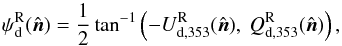6)result from the dispersion of B_POS around the mean direction of the large-scale GMF. The minus sign in ${\mathit{U}}_{\mathrm{d}\mathit{,}\mathrm{353}}^{\mathrm{R}}$ is necessary to produce angles in the IAU convention from HEALPix format Stokesmaps in the “COSMO” convention as used for the Planck data.

The mean normalized histogram of ${\mathit{\psi }}_{\mathrm{d}}^{\mathrm{R}}$ is computed from the multiple subsets of the Planck data and is presented in Fig.3 (blue inverted-triangles). The 1σ error bars on ${\mathit{\psi }}_{\mathrm{d}}^{\mathrm{R}}$ are derived from the standard deviation of the six independent measurements of the Planck data, as listed in Table1. We fit a Gaussian to the normalized histogram of ${\mathit{\psi }}_{\mathrm{d}}^{\mathrm{R}}$ and find a 1σ dispersion of over SGC34. Our 1σ dispersion value of ${\mathit{\psi }}_{\mathrm{d}}^{\mathrm{R}}$ is slightly higher than the one found over the high latitude southern Galactic cap (Planck Collaboration Int. XLIV 2016). This result is not unexpected because SGC34 extends up to b ≤ −30° and adopting a mean direction of the large-scale GMF is only an approximation.

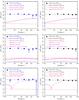Fig. 4 Left column: Planck 353GHz ${\mathrm{𝒟}}_{\mathit{\ell }}^{\mathit{EE}}$ (top row), ${\mathrm{𝒟}}_{\mathit{\ell }}^{\mathit{BB}}$ (middle row), and ${\mathrm{𝒟}}_{\mathit{\ell }}^{\mathit{TE}}$ (bottom row) power spectra in units of ${\mathit{\mu K}}_{\mathrm{CMB}}^{\mathrm{2}}$ computed over SGC34 using the subsets of the Planck data. See text calculation of 1σ error bars. The best-fit power law assuming exponent −2.3 is plotted for each power spectrum (dashed blue line). For comparison, we also show the Planck 2015 best-fit ΛCDM expectation curves for the CMB signal (Planck Collaboration XIII 2016), with the TE expectation shown as dashed where it is negative. Extrapolations of the dust power spectra to 150GHz (see text) are plotted as dashed red lines. Right column: similar to left panels, but for the dust model (Sect.5.4).

3.3. Polarized dust power spectra

We extend the analysis by Planck Collaboration Int. XXX (2016) of the region LR24 (${\mathit{f}}_{\mathrm{sky}}^{\mathrm{eff}}$=0.24 or 24% of the total sky) to the smaller lower column density selected area SGC34 within it (${\mathit{f}}_{\mathrm{sky}}^{\mathrm{eff}}$=0.085). We compute the polarized dust power spectra ${\mathrm{𝒟}}_{\mathit{\ell }}^{\mathit{EE}}$, ${\mathrm{𝒟}}_{\mathit{\ell }}^{\mathit{BB}}$, and ${\mathrm{𝒟}}_{\mathit{\ell }}^{\mathit{TE}}$ by cross-correlating the subsets of the Planck data at 353GHz in the multipole range 40 <ℓ< 160 over SGC34. We use the same D₃₅₃ map for all subsets of the Planck data. The binning of the measured power spectra in six multipole bins matches that used in Planck Collaboration Int. XXX (2016). We take the mean power spectra computed from the cross-spectra of DetSets (DS1×DS2), HalfMissions (HM1×HM2), and Years (Y1 × Y2). The mean dust ${\mathrm{𝒟}}_{\mathit{\ell }}^{\mathit{EE}}$ is corrected for the CMB contribution using the Planck best-fit ΛCDM model at the power spectrum level, while the mean ${\mathrm{𝒟}}_{\mathit{\ell }}^{\mathit{BB}}$ and ${\mathrm{𝒟}}_{\mathit{\ell }}^{\mathit{TE}}$ are kept unaltered. Figure4 shows that the contribution of the CMB BB spectra (for r = 0.15 with lensing contribution) is negligibly small as compared to the mean dust spectra ${\mathrm{𝒟}}_{\mathit{\ell }}^{\mathit{BB}}$ over SGC34. The mean ${\mathrm{𝒟}}_{\mathit{\ell }}^{\mathit{TE}}$ is unbiased because we use D₃₅₃ as a dust-only StokesI map. However, the unsubtracted CMB E-modes bias the 1σ error of the dust ${\mathrm{𝒟}}_{\mathit{\ell }}^{\mathit{TE}}$ power spectrum by a factor $\sqrt{\mathrm{\left[}{\mathrm{𝒟}}_{\mathit{\ell }}^{\mathit{TT}}\mathrm{\right(}\mathrm{dust}\mathrm{)}\mathrm{\times }{\mathrm{𝒟}}_{\mathit{\ell }}^{\mathit{EE}}\mathrm{(}\mathrm{CMB}\mathrm{\left)}\mathrm{\right]}\mathit{/}{\mathit{\nu }}_{\mathit{\ell }}}$, where ν_ℓ is associated with the effective number of degrees of freedom (Tristram et al. 2005).

The mean dust power spectra ${\mathrm{𝒟}}_{\mathit{\ell }}^{\mathit{EE}}$, ${\mathrm{𝒟}}_{\mathit{\ell }}^{\mathit{BB}}$, and ${\mathrm{𝒟}}_{\mathit{\ell }}^{\mathit{TE}}$ of the Planck 353GHz data are presented in the left column of Fig.4. The 1σ statistical uncertainties from noise (solid error bar in the left column of Fig.4) are computed from the analytical approximation implemented in Xpol. The 1σ systematic uncertainties are computed using the standard deviation of the dust polarization power spectra from the three subsets of the Planck data (as listed in Table1). The total 1σ error bar per ℓ bin (dashed error bar in the left column of Fig.4) is the quadrature sum of the two. The measured Planck 353GHz polarized dust power spectra ${\mathrm{𝒟}}_{\mathit{\ell }}^{\mathit{EE}}$, ${\mathrm{𝒟}}_{\mathit{\ell }}^{\mathit{BB}}$, and ${\mathrm{𝒟}}_{\mathit{\ell }}^{\mathit{TE}}$ are well described by power laws in multipole space, consistent with the one measured at intermediate and high Galactic latitudes (Planck Collaboration Int. XXX 2016). Similar to the analysis in Planck Collaboration Int. XXX (2016), we fit the power spectra with the power-law model, 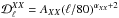${\mathrm{𝒟}}_{\mathit{\ell }}^{\mathit{XX}}\mathrm{=}{\mathit{A}}_{\mathit{XX}}\mathrm{(}\mathit{\ell }\mathit{/}\mathrm{80}{\mathrm{)}}^{{\mathit{\alpha }}_{\mathit{XX}}\mathrm{+}\mathrm{2}}$, where A_XX is the best-fit amplitude at ℓ = 80, α_XX is the best-fit slope, and XX = { EE,BB,TE }. We restrict the fit to six band-powers in the range 40 <ℓ< 160 so that we can compare the Planck data directly with the low-resolution dust model derived using the GASS H I data. The exponents α_XX of the unconstrained fits are quoted in the top row of Table2. Next, we perform the fit with a fixed exponent −2.3 for the appropriate α_XX. The resulting power laws are shown in the left column of Fig.4 and the values of χ² (with number of degrees of freedom, N_d.o.f. = 6) and the best-fit values of A_XX are presented in Table2.

The ratio of the dust B- and E-mode power amplitudes, roughly equal to a half (Table2), is maintained from LR24 to SGC34. The measured amplitude A_BB = 8.85 μK_CMB² at ℓ = 80 is about ~35% lower than the value expected from the empirical power-law A_BB ∝ ⟨ D₃₅₃ ⟩ ^1.9 (Planck Collaboration Int. XXX 2016) applied to SGC34. For future work, it will be important to understand the amplitude and variations of the dust B-mode signal in these low column density regions.

We find a significant positive TE correlation, ${\mathrm{𝒟}}_{\mathit{\ell }}^{\mathit{TE}}$, over SGC34; the amplitude A^TE normalized at ℓ = 80 hasmore than 4σ significance when the multipoles between 40 and 160 are combined in this way. Similarly, a positive TE correlation was reported over LR24 (see Fig.B.1 of Planck Collaboration Int. XXX 2016). The non-zero positive TE correlation is a direct consequence of the correlation between the dust intensity structures and the orientation of the magnetic field. Planck Collaboration Int. XXXVIII (2016) report that oriented stacking of the dust E-map over T peaks of interstellar filaments identified in the dust intensity map picks up a positive TE correlation (see their Fig.10).

For comparison in Fig.4 we show the Planck 2015 best-fit ΛCDM CMB ${\mathrm{𝒟}}_{\mathit{\ell }}^{\mathit{EE}}$, ${\mathrm{𝒟}}_{\mathit{\ell }}^{\mathit{BB}}$ (primordial tensor-to-scalar ratio r = 0.15 plus lensing contribution), and ${\mathrm{𝒟}}_{\mathit{\ell }}^{\mathit{TE}}$ expectation curves (Planck Collaboration XIII 2016). Then assuming that the dust spectral energy distribution (SED) follows a MBB spectrum with a mean dust spectral index 1.59 ± 0.02 and a mean dust temperature of 19.6K (Planck Collaboration Int. XXII 2015), we extrapolate the best-fit dust power spectra from 353GHz to 150GHz (scaling factor s_150/353 = 0.0408²) in order to show the level of the dust polarization signal (red dashed lines in Fig.4) relative to the CMB signal over SGC34.

4. Model framework

In this section we extend the formalism developed in Planck Collaboration Int. XLIV (2016) to simulate the dust polarization over SGC34 using a phenomenological description of the magnetic field and the GASS H I emission data. We introduce two main ingredients in the dust model: (1) fluctuations in the GMF orientation along the LOS and (2) alignment of the CNM structures with B_POS. Based on the filament study by Planck Collaboration Int. XXXVIII (2016), we anticipate that alignment of the CNM structures with B_POS will account for the positive dust TE correlation and the ${\mathrm{𝒟}}_{\mathit{\ell }}^{\mathit{TE}}$/${\mathrm{𝒟}}_{\mathit{\ell }}^{\mathit{EE}}$ ratio over SGC34.

4.1. Formalism

We use the general framework introduced by Planck Collaboration Int.XX (2015) to model the dust Stokesparameters, I, Q, and U, for optically thin regions at a frequencyν: $\begin{array}{ccc}& & {\mathit{I}}_{\mathrm{m}\mathit{,\nu }}\mathrm{\left(}\hat{{n}}\mathrm{\right)}\mathrm{=}\mathrm{\int }\left[\mathrm{1}\mathrm{-}{\mathit{p}}_{\mathrm{0}}\left({\cos }^{\mathrm{2}}{\mathit{\gamma }}^{\mathit{i}}\mathrm{\left(}\hat{{n}}\mathrm{\right)}\mathrm{-}\frac{\mathrm{2}}{\mathrm{3}}\right)\right]{\mathit{S}}_{\mathit{\nu }}^{\mathit{i}}\mathrm{\left(}\hat{{n}}\mathrm{\right)}\mathrm{d}{\mathit{\tau }}_{\mathit{\nu }}\\ & & \\ & & {\mathit{U}}_{\mathrm{m}\mathit{,\nu }}\mathrm{\left(}\hat{{n}}\mathrm{\right)}\mathrm{=}\mathrm{-}\mathrm{\int }{\mathit{p}}_{\mathrm{0}}{\cos }^{\mathrm{2}}{\mathit{\gamma }}^{\mathit{i}}\mathrm{\left(}\hat{{n}}\mathrm{\right)}\sin \mathrm{2}{\mathit{\psi }}^{\mathit{i}}\mathrm{\left(}\hat{{n}}\mathrm{\right)}{\mathit{S}}_{\mathit{\nu }}^{\mathit{i}}\mathrm{\left(}\hat{{n}}\mathrm{\right)}\mathrm{d}{\mathit{\tau }}_{\mathit{\nu }}\mathit{,}\end{array}$(7)where (see Appendix B of Planck Collaboration Int. XX 2015, for details) $\hat{{n}}$ is the direction vector, S_ν is the source function given by the relation S_ν = n_dB_ν(T)C_avg, τ_ν is the optical depth, p₀ = p_dustR is the product of the “intrinsic dust polarization fraction” (p_dust) and the Rayleigh reduction factor (R, related to the alignment of dust grains with respect to the GMF), ψ is the polarization angle measured from Galactic North, and γ is the angle between the local magnetic field and the POS. Again, like in Sect.3.2, the minus sign in U_m,ν is necessary to work from the angle map ψ given in the IAU convention to produce HEALPix format Stokesmaps in the COSMO convention. We start with the same dust Stokesparameters equations as in the Vansyngel et al. (2017) parametric dust model.

Following the approach in Planck Collaboration Int. XLIV (2016), we replace the integration along the LOS over SGC34 by the sum over a finite number of layers with different polarization properties. These layers are a phenomenological means of accounting for the effects of fluctuations in the GMF orientation along the LOS, the first main ingredient of the dust model. We interpret these layers along the LOS as three distinct phases of the ISM. The Gaussian decomposition of total N_Hi into the CNM, UNM, and WNM components based on their line-widths (or velocity dispersion) is described in detail in Sect.2.2.

We can replace the integral of the source function over each layer directly with the product of the column density maps of the three H I components and their mean dust emissivities. Within these astrophysical approximations, we can modify Eq.(7)to be $\begin{array}{ccc}{\mathit{I}}_{\mathrm{m}\mathit{,\nu }}\mathrm{\left(}\hat{{n}}\mathrm{\right)}& \mathrm{=}& \sum _{\mathit{i}\mathrm{=}\mathrm{1}}^{\mathrm{3}}\left[\mathrm{1}\mathrm{-}{\mathit{p}}_{\mathrm{0}}\left({\cos }^{\mathrm{2}}{\mathit{\gamma }}^{\mathit{i}}\mathrm{\left(}\hat{{n}}\mathrm{\right)}\mathrm{-}\frac{\mathrm{2}}{\mathrm{3}}\right)\right]\mathrm{⟨}{\mathit{ϵ}}_{\mathit{\nu }}^{\mathit{i}}\mathrm{⟩}{\mathit{N}}_{\mathrm{H}\hspace{0.17em}{i}}^{\mathit{i}}\mathrm{\left(}\hat{{n}}\mathrm{\right)}\\ {\mathit{Q}}_{\mathrm{m}\mathit{,\nu }}\mathrm{\left(}\hat{{n}}\mathrm{\right)}& \mathrm{=}& \\ {\mathit{U}}_{\mathrm{m}\mathit{,\nu }}\mathrm{\left(}\hat{{n}}\mathrm{\right)}& \mathrm{=}& \mathrm{-}\sum _{\mathit{i}\mathrm{=}\mathrm{1}}^{\mathrm{3}}{\mathit{p}}_{\mathrm{0}}{\cos }^{\mathrm{2}}{\mathit{\gamma }}^{\mathit{i}}\mathrm{\left(}\hat{{n}}\mathrm{\right)}\sin \mathrm{2}{\mathit{\psi }}^{\mathit{i}}\mathrm{\left(}\hat{{n}}\mathrm{\right)}\mathrm{⟨}{\mathit{ϵ}}_{\mathit{\nu }}^{\mathit{i}}\mathrm{⟩}{\mathit{N}}_{\mathrm{H}\hspace{0.17em}{i}}^{\mathit{i}}\mathrm{\left(}\hat{{n}}\mathrm{\right)}\mathit{,}\end{array}$(8)where $\mathrm{⟨}{\mathit{ϵ}}_{\mathit{\nu }}^{\mathit{i}}\mathrm{⟩}$ is the mean dust emissivity for each of the three H Icomponents.

In general, the emissivity is a function not only of frequency, but also of sky position $\hat{{n}}$ and different H I phases. However, in SGC34 the overall emissivity D₃₅₃/N_Hi is quite uniform (see Sect.5.2) and from a simultaneous fit of the D₃₅₃ map to all three component N_Hi maps we find little evidence, for our decomposition, that the emissivities of the individual components are different than the overall mean.

Similarly, the effective degree of alignment p₀ = p_dustR could be a function of frequency and different for different H I components. Equation(8)also tells us that the product p₀ is degenerate with ⟨ ϵ_ν ⟩ for the dust StokesQ_m,ν and U_m,ν parameters. Such effects could make the source functions in the layers even more different from one another.

In this paper we explore how models based on simplifying assumptions, namely a constant p₀ and a frequency dependent⟨ ϵ_ν ⟩ common to the three H I components, might despite the reduced flexibility nevertheless provide a good description of the data.

This use of the GASS N_Hi data can be contrasted to the approach of Planck Collaboration Int. XLIV (2016) and Vansyngel et al. (2017), where the source functions are assumed to be the same in each layer. Furthermore, Planck Collaboration Int. XLIV (2016) choose to ignore the correction term involving p₀ in the integrand for ${\mathit{I}}_{\mathrm{m}\mathit{,\nu }}\mathrm{\left(}\hat{{n}}\mathrm{\right)}$.

This phenomenological dust model based on the GASS H I data is not unique. It is based on several astrophysical assumptions as noted in this section. Within the same general framework, we could contemplate replacing the H I emission with three-dimensional (3D) extinction maps, though no reliable maps are currently available over the SGC34 region (Green et al. 2015). Furthermore, the HI emission traces the temperature or density structure of the diffuse ISM, whereas the dust extinction traces only the dust column density. Thus, using the HI emission to model the dust polarization is an interesting approach even if we had reliable 3D extinction maps toward the southern Galactic cap.

4.2. Structure of the Galactic magnetic field

The Galactic magnetic field, B, is expressed as a vector sum of a mean large-scale (ordered, B_ord) and a turbulent (random, B_turb) component (Jaffe et al. 2010) 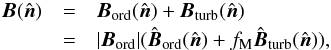$\begin{array}{ccc}{B}\mathrm{\left(}\hat{{n}}\mathrm{\right)}& \mathrm{=}& {{B}}_{\mathrm{ord}}\mathrm{\left(}\hat{{n}}\mathrm{\right)}\mathrm{+}{{B}}_{\mathrm{turb}}\mathrm{\left(}\hat{{n}}\mathrm{\right)}\\ & \mathrm{=}& \end{array}$(9)where f_M is the standard deviation of the relative amplitude of the turbulent component | B_turb | with respect to the mean large-scale | B_ord |. The butterfly patterns seen in the orthographic projections of the Planck polarization maps, Q_d,353 and U_d,353, centred at (l,b) = (0°,−90°) are well fitted by a mean direction of the large-scale GMF over the southern Galactic cap (Planck Collaboration Int. XLIV 2016). We assume that the mean direction of the large-scale GMF is still a good approximation to fit the butterfly patterns seen in the Planck StokesQ_d,353 and U_d,353 maps over SGC34 (Fig.1). The unit vector $\hat{{B}}{\mathrm{ord}}_{}$ is defined as $\hat{{B}}{}_{\mathrm{ord}}\mathrm{=}\mathrm{\left(}\cos {\mathit{l}}_{\mathrm{0}}\cos {\mathit{b}}_{\mathrm{0}}\mathit{,}\sin {\mathit{l}}_{\mathrm{0}}\cos {\mathit{b}}_{\mathrm{0}}\mathit{,}\sin {\mathit{b}}_{\mathrm{0}}\mathrm{\right)}$.

We model B_turb with a Gaussian realization on the sky with an underlying power spectrum, C_ℓ ∝ ℓ^α_M, for ℓ ≥ 2 (Planck Collaboration Int. XLIV 2016). The correlated patterns of B_turb over the sky are needed to account for the correlated patterns of dust p and ψ seen in Planck 353GHz data (Planck Collaboration Int. XIX 2015). Following Fauvet et al. (2012), we only consider isotropic turbulence in our analysis. We produce a spatial distribution of B_turb in the x, y, and z direction from the above power spectrum on the celestial sphere of HEALPix resolution N_side. We add B_turb to B_ord with a relative strength f_M as given in Eq.(9).

4.3. Alignment of the CNM structures with the magnetic field

We use the algebra given in Sect.4.1 of Planck Collaboration Int.XLIV (2016) to compute cos²γⁱ for the three H I components. For the UNM and WNM components, we assume that there is no TE correlation and the angles ψ^u and ψ^w are computed directly from the total B again using the algebra by Planck Collaboration Int. XLIV (2016). For the CNM we follow a quite different approach to compute ψ^c.

We introduce a positive TE correlation for the CNM component through the polarization angle ψ^c. The alignment between the CNM structures and B_POS is introduced to test whether it fully accounts for the observed E-B power asymmetry or not. To do that, we assume that the masked ${\mathit{N}}_{{Hi}}^{\mathrm{c}}$ map is a pure E-mode map and define spin-2 maps Q_T and U_T as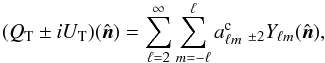$\mathrm{(}{\mathit{Q}}_{\mathrm{T}}\mathrm{\pm }\mathit{i}{\mathit{U}}_{\mathrm{T}}\mathrm{)}\mathrm{\left(}\hat{{n}}\mathrm{\right)}\mathrm{=}\sum _{\mathit{\ell }\mathrm{=}\mathrm{2}}^{\mathrm{\infty }}\sum _{\mathit{m}\mathrm{=}\mathrm{-}\mathit{\ell }}^{\mathit{\ell }}{\mathit{a}}_{\mathit{\ell m}}^{\mathrm{c}}{\mathrm{\pm }\mathrm{2}}_{}{\mathit{Y}}_{\mathit{\ell m}}\mathrm{\left(}\hat{{n}}\mathrm{\right)}\mathit{,}$(10)where ${\mathit{a}}_{\mathit{\ell m}}^{\mathrm{c}}$are the harmonic coefficients of the masked ${\mathit{N}}_{{Hi}}^{\mathrm{c}}$map. In the flat-sky limit, ${\mathit{Q}}_{\mathrm{T}}\mathrm{\simeq }\mathrm{(}{\mathit{\partial }}_{\mathrm{x}}^{\mathrm{2}}\mathrm{-}{\mathit{\partial }}_{\mathrm{y}}^{\mathrm{2}}\mathrm{)}{\mathrm{\nabla }}^{-2}{\mathit{N}}_{{Hi}}^{\mathrm{c}}$ and ${\mathit{U}}_{\mathrm{T}}\mathrm{\simeq }\mathrm{-}\mathrm{2}{\mathit{\partial }}_{\mathit{x}}{\mathit{\partial }}_{\mathit{y}}{\mathrm{\nabla }}^{-2}{\mathit{N}}_{{Hi}}^{\mathrm{c}}$, where ∇^-2 is the inverse Laplacian operator (Bowyer et al. 2011). We compute the angle ψ^c using the relation, ψ^c = (1/2)tan^-1(−U_T,Q_T) (see Planck Collaboration XVI 2016, for details). The polarization angle ψ^c is the same as the angle between the major axis defined by a local quadrature expansion of the ${\mathit{N}}_{{Hi}}^{\mathrm{c}}$ map and the horizontal axis. This idea of aligning perfectly the CNM structures with B_POS is motivated from the H I studies by Clark et al. (2015), Martin et al. (2015), and Kalberla et al. (2016), and Planck dust polarization studies by Planck Collaboration Int. XXXII (2016) and Planck Collaboration Int. XXXVIII (2016). This is the second main ingredient of the dust model.

4.4. Model parameters

The dust model has the following parameters: ⟨ ϵ_ν ⟩, the mean dust emissivity per H I component at frequency ν; p₀, the normalization factor to match the observed dust polarization fraction over the southern Galactic cap; l₀ and b₀, describing the mean direction of B_ord in the region of the southern Galactic cap; f_M, the relative strength of B_turb with respect to B_ord for the different components; α_M, the spectral index of B_turb power spectrum for the different components; and σ_c and σ_u to separate the total N_Hi into the CNM, UNM, and WNM components (phases).

We treat the three H I components with different density structures and magnetic field orientations as three independent layers. Because we include alignment of the CNM structures with B_POS, we treat the CNM polarization layer separately from the WNM and UNM polarization layers. The value of ${\mathit{f}}_{\mathrm{M}}^{\mathrm{c}}$ for the CNM component is different than the common ${\mathit{f}}_{\mathrm{M}}^{\mathrm{u}\mathit{/}\mathrm{w}}$ for the UNM and WNM components. For the same reason, the spectral index of the turbulent power spectrum ${\mathit{\alpha }}_{\mathrm{M}}^{\mathrm{c}}$ for the CNM component could be different than the common ${\mathit{\alpha }}_{\mathrm{M}}^{\mathrm{u}\mathit{/}\mathrm{w}}$ for the UNM and WNM components, but we take them to be the same, simplifying the model and reducing the parameter space in our analysis. We also use the same values of ⟨ ϵ_ν ⟩ and p₀ for each layer. This gives a total of nine parameters.

In this analysis, we do not optimize the nine parameters of the dust model explicitly. Instead, we determine five parameters based on various astrophysical constraints and optimize only⟨ ϵ_ν ⟩, p₀, ${\mathit{f}}_{\mathrm{M}}^{\mathrm{u}\mathit{/}\mathrm{w}}$, and σ_c simultaneously (Sect.5.2). Our main goal is to test quantitatively whether the fluctuations in the GMF orientation along the LOS plus the preferential alignment of the CNM structures with B_POS can account simultaneously for both the observed dust polarization power spectra and the normalized histograms of p² and ψ^R over SGC34.

We review here the relationship between the nine dust model parameters and the various dust observables.

• The emissivity ⟨ ϵ_ν ⟩ simply converts the observed N_Hi (10²⁰cm^-2) to the Planck intensity units (in μK_CMB) (Planck Collaboration Int. XVII 2014). This parameter is optimized in Sect.5.2, subject to a strong prior obtained by correlating the map D₃₅₃ with the N_Hi map.

• The parameter p₀ is constrained by the observed distribution of ${\mathit{p}}_{\mathrm{d}}^{\mathrm{2}}$ at 353GHz and the amplitude of the dust polarization power spectra ${\mathrm{𝒟}}_{\mathit{\ell }}^{\mathit{EE}}$, ${\mathrm{𝒟}}_{\mathit{\ell }}^{\mathit{BB}}$, and ${\mathrm{𝒟}}_{\mathit{\ell }}^{\mathit{TE}}$. It is optimized using the latter in Sect.5.2.

• The two model parameters l₀ and b₀ determine the orientation of the butterfly patterns seen in the orthographic projections of the Planck polarization maps, Q_d,353 and U_d,353 (Planck Collaboration Int. XLIV 2016). They are found by fitting these data (Sect.3.2).

• The parameter f_M for each polarization layer is related to the dispersion of ${\mathit{\psi }}_{\mathrm{d}}^{\mathrm{R}}$ and ${\mathit{p}}_{\mathrm{d}}^{\mathrm{2}}$ (the higher the strength of the turbulent field with respect to the ordered field, the higher the dispersion of ${\mathit{\psi }}_{\mathrm{d}}^{\mathrm{R}}$ and ${\mathit{p}}_{\mathrm{d}}^{\mathrm{2}}$) and to the amplitude of the dust polarization power spectra. Our prescription for the alignment of CNM structure and B_POS subject to statistical constraints from polarization data determines ${\mathit{f}}_{\mathrm{M}}^{\mathrm{c}}$ (Sect.5.1); ${\mathit{f}}_{\mathrm{M}}^{\mathrm{u}\mathit{/}\mathrm{w}}$ is optimized using the dust polarization band powers in Sect.5.2.

• The parameter ${\mathit{\alpha }}_{\mathrm{M}}^{\mathrm{c}}$ is constrained by the alignment of the CNM structures with B_POS (Sect.5.1).

• The parameter σ_c controls the fraction of the H I in the CNM and hence sets the amount of E-B power asymmetry and the ${\mathrm{𝒟}}_{\mathit{\ell }}^{\mathit{TE}}$/${\mathrm{𝒟}}_{\mathit{\ell }}^{\mathit{EE}}$ ratio through the alignment of the CNM structures with B_POS. It is optimized in Sect.5.2. Our dust model is insensitive to the precise value of the parameter σ_u, which is used to separate the UNM and WNM into distinct layers.

To break the degeneracy between different dust model parameters and obtain a consistent and robust model, we need to make use of dust polarization observables in pixel space as well as in harmonic space.

5. Dust sky simulations

We simulate the dust intensity and polarization maps at only a single Planck frequency 353GHz. It would be straightforward to extrapolate the dust model to other microwave frequencies using a MBB spectrum of the dust emission (Planck Collaboration Int.XVII 2014; Planck Collaboration Int.XXI 2015; Planck Collaboration Int. XXX 2016) or replacing the value of ⟨ ϵ_ν ⟩ from Planck Collaboration Int. XVII (2014). However, such a simple-minded approach would not generate any decorrelation of the dust polarization pattern between different frequencies, as reported in Planck Collaboration Int. L (2017).

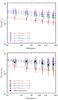Fig. 5 Mean power spectra of cos2γ (top panel) and cos2ψ (bottom panel) over SGC34 for a set of αM and fM parameters in the multipole range 40 <ℓ< 160. The 1σ error bars are computed from the standard deviations of the 100Monte-Carlo realizations of the dust model. The alignment of the CNM structures with BPOS (see Sect.5.1 for details) constrains the value of ${\mathit{\alpha }}_{\mathrm{M}}^{\mathrm{c}}$ and ${\mathit{f}}_{\mathrm{M}}^{\mathrm{c}}$ for the CNM component.

5.1. Constraining the turbulent GMF for the CNM component

As discussed in Sect.4.3, we adopted an alternative approach to compute the polarization angle ψ^c for the CNM component. At first sight, it might look physically inconsistent and therefore a main source of bias. However, we now show that the original and alternative approaches lead to statistically similar results and so can be compared in order to constrain the parameters of B_turb, that is ${\mathit{\alpha }}_{\mathrm{M}}^{\mathrm{c}}$ and ${\mathit{f}}_{\mathrm{M}}^{\mathrm{c}}$, for the CNM component.

To do this we first adopt the original approach from Planck Collaboration Int. XLIV (2016; and used for the UNM and CNM components). We generate Gaussian realizations of B_turb for a set of (α_M,f_M) values. We assume a fixed mean direction of B_ord as 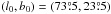(Table1) and add to it B_turb to derive a total B. We use the algebra given in Sect.4.1 of Planck Collaboration Int. XLIV (2016) to compute the two quantities cos²γ and cos2ψ for different values of α_M and f_M. Because the polarization angles γ and ψ are circular quantities, we choose to work with quantities like cos²γ and cos2ψ as they appear in the StokesQ and U parameters (Eq.(8)). We then apply the Xpol routine to compute the angular power spectra of these two quantities for each sky realization over SGC34. The mean power spectra of cos²γ and cos2ψ are computed by averaging 100Monte-Carlo realizations and are presented in Fig.5. The power spectra of the two polarization angles are well described by power-laws in multipole space, , where α_M is the same as the spectral index of B_turb power spectrum. The amplitudes and slopes of these two quantities are related systematically to the values of α_M and f_M. The higher the f_M value, the higher is the amplitude of the power spectra in Fig.5. The best-fit slope of the power spectrum over the multipole range 40 < ℓ < 160 is the same as the spectral index of the B_turb power spectrum for relevant f_M values.

For each Monte Carlo realization we also calculated ψ^c for the CNM component by the alternative approach and from that computed the power spectra of cos2ψ for the CNM component over SGC34. By comparing these results to the spectra from the first Planck Collaboration Int. XLIV (2016) approach, as in Fig.5 (bottom panel), we can constrain the values of ${\mathit{\alpha }}_{\mathrm{M}}^{\mathrm{c}}$ and ${\mathit{f}}_{\mathrm{M}}^{\mathrm{c}}$. The typical values of ${\mathit{\alpha }}_{\mathrm{M}}^{\mathrm{c}}$ and ${\mathit{f}}_{\mathrm{M}}^{\mathrm{c}}$ are −2.4 and 0.4, respectively. One needs a Monte-Carlo approach to put realistic error bars on the ${\mathit{\alpha }}_{\mathrm{M}}^{\mathrm{c}}$ and ${\mathit{f}}_{\mathrm{M}}^{\mathrm{c}}$ parameters, which is beyond the scope of this paper. However, we do note that the value of ${\mathit{\alpha }}_{\mathrm{M}}^{\mathrm{c}}$ is close to the exponent of the angular power spectrum of the ${\mathit{N}}_{{Hi}}^{\mathrm{c}}$ map computed over SGC34, reflecting the correlation between the structure of the intensity map and the orientation of the field.

We stress that the values of ${\mathit{\alpha }}_{\mathrm{M}}^{\mathrm{c}}$ and ${\mathit{f}}_{\mathrm{M}}^{\mathrm{c}}$ derived from Fig.5 are valid only over SGC34. If we increase the sky fraction to b ≤ −30° covered by the GASS H I survey, we get the same ${\mathit{\alpha }}_{\mathrm{M}}^{\mathrm{c}}$ value, but a slightly higher ${\mathit{f}}_{\mathrm{M}}^{\mathrm{c}}$ value (${\mathit{f}}_{\mathrm{M}}^{\mathrm{c}}\mathrm{=}\mathrm{0.5}$). This suggests that the relative strength of B_turb with respect to B_ord might vary across the sky.

5.2. Values of model parameters

Here we describe how the nine model parameters were found.

We found the mean direction of B_ord to be and from a simple model fit of normalized Stokesparameters for polarization over SGC34 (Sect.3.2, Table1).

As described in Sect.5.1, using ${\mathit{N}}_{{Hi}}^{\mathrm{c}}$ as a tracer of the dust polarization angle gives the constraints ${\mathit{\alpha }}_{\mathrm{M}}^{\mathrm{c}}\mathrm{=}\mathrm{-}\mathrm{2.4}$ and ${\mathit{f}}_{\mathrm{M}}^{\mathrm{c}}\mathrm{=}\mathrm{0.4}$. The spectral index ${\mathit{\alpha }}_{\mathrm{M}}^{\mathrm{u}\mathit{/}\mathrm{w}}$ of B_turb for the UNM and WNM components is assumed to be same as the ${\mathit{\alpha }}_{\mathrm{M}}^{\mathrm{c}}$ value of the CNM component, for simplicity.

Only four model parameters, ⟨ ϵ₃₅₃ ⟩, p₀, ${\mathit{f}}_{\mathrm{M}}^{\mathrm{u}\mathit{/}\mathrm{w}}$, and σ_c, are adjusted by evaluating the goodness of fit through a χ²-test, specifically ${\mathit{\chi }}_{\mathit{XX}}^{\mathrm{2}}\mathrm{=}\sum _{{\mathit{\ell }}_{\min }}^{{\mathit{\ell }}_{\max }}\left[\frac{{\mathrm{𝒟}}_{\mathit{\ell }}^{\mathit{XX}}\mathrm{-}{\mathrm{ℳ}}_{\mathit{\ell }}^{\mathit{XX}}\mathrm{(}\mathrm{⟨}{\mathit{ϵ}}_{\mathrm{353}}\mathrm{⟩}\mathit{,}{\mathit{p}}_{\mathrm{0}}\mathit{,}{\mathit{f}}_{\mathrm{M}}^{\mathrm{u}\mathit{/}\mathrm{w}}\mathit{,}{\mathit{\sigma }}_{\mathrm{c}}\mathrm{)}}{{\mathit{\sigma }}_{\mathit{\ell }}^{\mathit{XX}}}\right]2$(11)and ${\mathit{\chi }}^{\mathrm{2}}\mathrm{=}\sum _{\mathit{i}}^{{\mathit{N}}_{\mathrm{pix}}}{\mathrm{[}{\mathit{D}}_{\mathrm{353}}\mathrm{-}\mathit{s}{\mathit{I}}_{\mathrm{m}\mathit{,}\mathrm{353}}\mathrm{(}\mathrm{⟨}{\mathit{ϵ}}_{\mathrm{353}}\mathrm{⟩}\mathit{,}{\mathit{p}}_{\mathrm{0}}\mathit{,}{\mathit{f}}_{\mathrm{M}}^{\mathrm{u}\mathit{/}\mathrm{w}}\mathit{,}{\mathit{\sigma }}_{\mathrm{c}}\mathrm{)}\mathrm{-}{\mathit{o}}^{\mathrm{]}}}^{\mathrm{2}}\mathit{,}$(12)where XX = { EE,BB,TE }, ${\mathrm{𝒟}}_{\mathit{\ell }}^{\mathit{XX}}$, and ${\mathit{\sigma }}_{\mathit{\ell }}^{\mathit{XX}}$ are the mean observed dust polarization band powers and standard deviation at 353GHz, respectively, ${\mathrm{ℳ}}_{\mathit{\ell }}^{\mathit{XX}}$ is the model dust polarization power spectrum over SGC34, N_pix is the total number of pixels in SGC34, s and o are the slope and the offset of the “T-T” correlation between the D₃₅₃ and I_m,353 maps. We evaluated ${\mathit{\chi }}_{\mathit{XX}}^{\mathrm{2}}$ using the six band powers in the range 40 <ℓ < 160. For χ² minimization, we put a flat prior on the mean dust emissivity, ⟨ ϵ₃₅₃ ⟩ = (111 ± 22) μK_CMB(10²⁰ cm^-2)^-1 at 353GHz, as obtained by correlating N_Hi with D₃₅₃ map over SGC34. Based on the observed distribution of the polarization fraction (Sect.3.1), we put a flat prior on p₀ = (18 ± 4)%. To match the observed dust amplitude at 353GHz, the value of s should be close to 1 and is kept so by adjusting ⟨ ϵ₃₅₃ ⟩ during the iterative solution of the two equations.

The typical mean values of ⟨ ϵ₃₅₃ ⟩, p₀, ${\mathit{f}}_{\mathrm{M}}^{\mathrm{u}\mathit{/}\mathrm{w}}$, and σ_c that we obtained are 121.8 μK_CMB(10²⁰ cm^-2)^-1, 18.5%, 0.1, and 7.5kms^-1, respectively, with ${\mathit{\chi }}_{\mathit{EE}}^{\mathrm{2}}\mathrm{=}\mathrm{5.0}$, ${\mathit{\chi }}_{\mathit{BB}}^{\mathrm{2}}\mathrm{=}\mathrm{3.3}$, and ${\mathit{\chi }}_{\mathit{TE}}^{\mathrm{2}}\mathrm{=}\mathrm{4.9}$ for six degrees of freedom (or band-powers). The precise optimization is not important and is beyond the scope of this paper.

The model is not particularly sensitive to the value of the final parameter, σ_u, but it is important to have significant column density in each of UNM and WNM so as to have contributions from three layers; we chose σ_u = 10kms^-1, for which the average column densities of the phases over SGC34 are rather similar (Sect.2.3).

Our value of ⟨ ϵ₃₅₃ ⟩ differs slightly from the mean value ⟨ ϵ₃₅₃ ⟩ quoted in Table2 of Planck Collaboration Int. XVII (2014), where the Planck intensity maps are correlated with HI LVC emission over many patches within Galactic latitude b< −25°. A difference in the mean dust emissivity is not unexpected because our study is focussed on the low column density region (N_{H i} ≤ 2.7 × 10²⁰ cm^-2) within the Planck Collaboration Int. XVII (2014) sky region (N_{H i} ≤ 6 × 10²⁰ cm^-2).

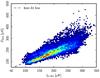Fig. 6 Correlation of the Planck 353GHz dust intensity map and the dust model StokesI map. The dashed line is the best-fit relation.

Figure6 shows the correlation between the data D₃₅₃ and the model I_m,353 over SGC34. The parameters of the best fit line are s = 1.0 (iteratively by construction) and o = −6.6 μK_CMB. We compute a residual map Δ ≡ D₃₅₃−I_m,353 over SGC34. The dispersion of the residual emission with respect to the total D₃₅₃ emission is σ_Δ/σ_D353 = 0.36. This means that the residual emission accounts for only 13% (${\mathit{\sigma }}_{\mathrm{\Delta }}^{\mathrm{2}}\mathit{/}{\mathit{\sigma }}_{{\mathit{D}}_{\mathrm{353}}}^{\mathrm{2}}$) of the total dust power at 353 GHz. We calculate the Pearson correlation coefficients over SGC34 between the residual map and the three H I templates, namely the CNM, UNM, and WNM, finding −0.09, −0.17, and 0.13, respectively. The residual might originate in pixel-dependent variations of ϵ₃₅₃ or possibly from diffuse ionized gas that is not spatially correlated with the total N_Hi map. Planck Collaboration Int. XVII (2014) explored these two possibilities (see their Appendix D) and were able to reproduce the observed value of σ_Δ/ ⟨ D₃₅₃ ⟩ at 353GHz. We do not use the residual emission in our analysis because our main goal is to reproduce the mean dust polarization properties over the SGC34 region. For future work, the pixel-dependent variation of ϵ₃₅₃, like in the Planck Collaboration Int. XVII (2014) analysis, could be included so that one could compare the refined dust model with the observed dust polarization data for a specific sky patch (e.g. the BICEP2 field).

5.3. Monte-Carlo simulations

Using the general framework described in Sect.4, we simulate a set of 100 polarized dust sky realizations at 353GHz using a set of model parameters, as discussed in Sect.4.4. Because the model of the turbulent GMF is statistical, we can simulate multiple dust sky realizations for a given set of parameters. The simulated dust intensity and polarization maps are smoothed to an angular resolution of FWHM 1° and projected on a HEALPix grid of N_side=128. These dust simulations are valid only in the low column density regions.

To compare the dust model with the Planck observations, we add realistic noise simulations called full focal plane 8 or “FFP8” (Planck Collaboration XII 2016). These noise simulations include the realistic noise correlation between pair of detectors for a given bolometer. For a given dust realization, we produce two independent samples of dust StokesQ and U noisy model maps as 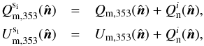$\begin{array}{ccc}{\mathit{Q}}_{\mathrm{m}\mathit{,}\mathrm{353}}^{{\mathrm{s}}_{\mathrm{i}}}\mathrm{\left(}\hat{{n}}\mathrm{\right)}& \mathrm{=}& {\mathit{Q}}_{\mathrm{m}\mathit{,}\mathrm{353}}\mathrm{\left(}\hat{{n}}\mathrm{\right)}\mathrm{+}{\mathit{Q}}_{\mathrm{n}}^{\mathit{i}}\mathrm{\left(}\hat{{n}}\mathrm{\right)}\mathit{,}\\ {\mathit{U}}_{\mathrm{m}\mathit{,}\mathrm{353}}^{{\mathrm{s}}_{\mathrm{i}}}\mathrm{\left(}\hat{{n}}\mathrm{\right)}& \mathrm{=}& \end{array}$(13)where i = 1,2 are two independent samples, and ${\mathit{Q}}_{\mathrm{n}}^{\mathit{i}}$ and ${\mathit{U}}_{\mathrm{n}}^{\mathit{i}}$ are the statistical noise of the subsets of the Planck polarization maps (as listed in Table1).

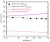Fig. 7 Best-fit power law dust model TT power spectra at 353GHz (black dashed line) and extrapolated dust power spectra at 150GHz (red dashed line) as computed over SGC34. For comparison, we also show the Planck 2015 best-fit ΛCDM expectation curves of the CMB signal.

5.4. Comparison of the dust model with Planck observations

In this section we compare the statistical properties of the dust polarization from the dust model with the Planck 353GHz observations over the selected region SGC34.

We showed in Fig.6 that the model Stokes${\mathit{I}}_{\mathrm{353}}^{\mathrm{m}}$ provides a good fit to the D₃₅₃ map in amplitude. Here we show that this is the case for the shape of the ${\mathrm{𝒟}}_{\mathit{\ell }}^{\mathit{TT}}$ power spectrum too. We compute the model dust TT power spectrum, ${\mathrm{ℳ}}_{\mathit{\ell }}^{\mathit{TT}}\mathrm{\equiv }\mathit{\ell }\mathrm{(}\mathit{\ell }\mathrm{+}\mathrm{1}\mathrm{)}{\mathit{C}}_{\mathit{\ell ,}\mathrm{m}}^{\mathit{TT}}\mathit{/}\mathrm{\left(}\mathrm{2}\mathit{\pi }\mathrm{\right)}$, over SGC34 in the range 40 <ℓ< 600. The dust ${\mathrm{ℳ}}_{\mathit{\ell }}^{\mathit{TT}}$ power spectrum is well represented with a power-law model, ${\mathrm{ℳ}}_{\mathit{\ell }}^{\mathit{TT}}\mathrm{\propto }\mathrm{(}\mathit{\ell }\mathit{/}\mathrm{80}{\mathrm{)}}^{{\mathit{\alpha }}_{\mathit{TT}}\mathrm{+}\mathrm{2}}$, with a best-fit slope α_TT = −2.59 ± 0.02, as shown in Fig.7. Our derived best-fit value of α_TT is consistent with that measured in Planck Collaboration XVI (2014) and Planck Collaboration XIII (2016) at high Galactic latitude. For comparison, we also show the TT power spectrum of the CMB signal for the Planck 2015 best-fit ΛCDM model (Planck Collaboration XIII 2016). The best-fit dust ${\mathrm{ℳ}}_{\mathit{\ell }}^{\mathit{TT}}$ power spectrum extrapolated from 353GHz to 150GHz, scaling as in Fig.4 and shown here as a dashed red line, reveals that over SGC34 the amplitude of the dust emission at 150GHz is less than 1% compared to the amplitude of the CMB signal.

Next we show that the dust model is able to reproduce the observed distribution on ${\mathit{p}}_{\mathrm{d}}^{\mathrm{2}}$ and dispersion of ${\mathit{\psi }}_{\mathrm{d}}^{\mathrm{R}}$ over SGC34 shown in Figs.2 and 3. We note that these statistics were not used to optimize the four model parameters in Sect.5.2, and so this serves as an important quality check for the model. We compute the square of the polarization fraction, ${\mathit{p}}_{\mathrm{m}}^{\mathrm{2}}$, for the dust model ${\mathit{p}}_{\mathrm{m}}^{\mathrm{2}}\mathrm{=}⟨\frac{{\mathit{Q}}_{\mathrm{m}\mathit{,}\mathrm{353}}^{{\mathrm{s}}_{\mathrm{1}}}{\mathit{Q}}_{\mathrm{m}\mathit{,}\mathrm{353}}^{{\mathrm{s}}_{\mathrm{2}}}\mathrm{+}{\mathit{U}}_{\mathrm{m}\mathit{,}\mathrm{353}}^{{\mathrm{s}}_{\mathrm{1}}}{\mathit{U}}_{\mathrm{m}\mathit{,}\mathrm{353}}^{{\mathrm{s}}_{\mathrm{2}}}}{{\mathit{I}}_{\mathrm{m}\mathit{,}\mathrm{353}}^{\mathrm{2}}}⟩\mathit{,}$(14)where the index “m” again refers to the dust model. We use the two independent samples to exploit the statistical independence of the noise between them. The mean normalized histogram of ${\mathit{p}}_{\mathrm{m}}^{\mathrm{2}}$ and the associated 1σ error bars are computed over SGC34 using 100 Monte-Carlo simulations. Returning to Fig.2, we compare the normalized histogram of ${\mathit{p}}_{\mathrm{m}}^{\mathrm{2}}$ (black circles) with the normalized histogram of ${\mathit{p}}_{\mathrm{d}}^{\mathrm{2}}$ (blue inverted-triangles). The Planck instrumental noise (FFP8 noise) added in the dust model accounts nicely for the observed negative values of ${\mathit{p}}_{\mathrm{m}}^{\mathrm{2}}$ and also contributes the extension of the ${\mathit{p}}_{\mathrm{m}}^{\mathrm{2}}$ distribution beyond the input value of ${\mathit{p}}_{\mathrm{0}}^{\mathrm{2}}$. The value of p₀ found in this paper is close to the value of 19% deduced at 1° resolution over intermediate and low Galactic latitudes (Planck Collaboration Int. XIX 2015).

We also compute the dispersion of the polarization angle${\mathit{\psi }}_{\mathrm{m}}^{\mathrm{R}}$ for the dust model. We follow the same procedure as discussed in Sect.3.3 and compute the angle ${\mathit{\psi }}_{\mathrm{m}}^{\mathrm{R}}\mathrm{=}\frac{\mathrm{1}}{\mathrm{2}}{\tan }^{-1}\mathrm{(}\mathrm{-}{\mathit{U}}_{\mathrm{m}\mathit{,}\mathrm{353}}^{\mathrm{R}}\mathit{,}{{\mathit{Q}}_{\mathrm{m}\mathit{,}\mathrm{353}}^{\mathrm{R}}}^{\mathrm{)}}\mathit{,}$(15)where ${\mathit{Q}}_{\mathrm{m}\mathit{,}\mathrm{353}}^{\mathrm{R}}$ and ${\mathit{U}}_{\mathrm{m}\mathit{,}\mathrm{353}}^{\mathrm{R}}$ are rotated Stokesparameters with respect to the local direction of the large-scale GMF. We make the normalized histogram of ${\mathit{\psi }}_{\mathrm{m}}^{\mathrm{R}}$ over SGC34. The mean normalized histogram and associated 1σ error bars of ${\mathit{\psi }}_{\mathrm{m}}^{\mathrm{R}}$ for the dust model are computed from 100 Monte-Carlo simulations. Returning to Fig.3, we compare the dispersion of ${\mathit{\psi }}_{\mathrm{m}}^{\mathrm{R}}$ (black points) with the dispersion of ${\mathit{\psi }}_{\mathrm{d}}^{\mathrm{R}}$ (blue points). The 1σ dispersion of ${\mathit{\psi }}_{\mathrm{m}}^{\mathrm{R}}$ derived from the mean of 100 dust model realizations is , slightly larger than for the Planck data ( , Sect.3.2). This could come from the simple modelling assumptions used in our analysis. In particular, the histograms of ${\mathit{p}}_{\mathrm{d}}^{\mathrm{2}}$ and ${\mathit{\psi }}_{\mathrm{d}}^{\mathrm{R}}$ depend on the dust modelling at low multipoles (ℓ< 40), which are not constrained by our data fitting. Varying some of the model parameters such as ${\mathit{\alpha }}_{\mathrm{M}}^{\mathrm{u}\mathit{/}\mathrm{w}}$, different R for different ISM phases, or introducing a low-ℓ cutoff in the spectral index of the B_turb (Cho & Lazarian 2002, 2010) might provide a better fit of these histograms to the Planck data. Due to the limited sky coverage over SGC34 and residual systematics in the publicly available Planck PR2 data at low multipoles (Planck Collaboration Int. XLVI 2016), we are unable to test some of these possibilities within our modelling framework.

Finally, we compute power spectra of the dust model over SGC34 using the cross-spectra of two independent samples as described in Sects.3.3 and 5.3. Mean dust polarization power spectra of the noisy dust model, ${\mathrm{ℳ}}_{\mathit{\ell }}^{\mathit{EE}}$, ${\mathrm{ℳ}}_{\mathit{\ell }}^{\mathit{BB}}$, and ${\mathrm{ℳ}}_{\mathit{\ell }}^{\mathit{TE}}$, over the multipole range 40 < ℓ < 160 are calculated from 100Monte-Carlo simulations and presented in the right column of Fig.4. The associated 1σ error bar per ℓ bin is also derived from the Monte-Carlo simulations. All of the dust polarization power spectra are well represented by a power law in ℓ. We fit the model spectra with a power-law model over the multipole range 40 < ℓ < 160. The best-fit values of the exponents and then of the amplitudes with exponent −2.3 are quoted in Table2. Because of the χ² optimization of the four model parameters (Sect.5.2), these power spectra agree well with the observed power spectra over SGC34.

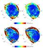Fig. 8 Left column: orthographic projections of the Planck 353GHz D353 (StokesI) map (top row) and the square of the polarization intensity P2 (bottom row), at 1° resolution over the southern Galactic cap covered by the GASS H I survey, with the selected region SGC34 outlined by a black contour. The same coordinate system is used as in Fig.1. Right column: similar to left panels, but for a realization of the 353GHz dust model. Judged visually, the dust model is able to reproduce roughly the observed dust polarization sky over SGC34, and indeed over the entire field shown.

6. Predictions from the dust model

The simulated dust emission maps with FFP8 noise approximate the Planck 353GHz data well over SGC34. In this section we use noiseless dust simulations to make a few predictions concerning the foreground dust B-mode that are important for the search for the CMB B-mode signal. These predictions include the TB and EB correlation for the dust emission and the statistical variance of the dust B-modes at the power spectrum level.

But first we compare the spatial distribution of StokesI and the polarization intensity (P²) of the noiseless dust model with the Planck 353GHz data over the southern Galactic cap. The comparison between one realization of the dust model and the Planck data is presented in Fig.8. The dust simulation is derived completely from the GASS HI data and a phenomenological description of the large-scale and turbulent components of the GMF with parameters optimized over SGC34, a subregion of the SGC. We find a good match between the data and the dust model over SGC34, outlined by the black contour. Outside of SGC34, the brightest emission features appear stronger in the Planck 353GHz data because the HI-based dust model does not account for dust emission associated with H₂ gas and with H I gas that is too cold to result in significant net emission.

6.1. Dust TB and EB correlation

The TB and EB cross-spectra vanish for the CMB signal in the standard ΛCDM model (Zaldarriaga & Seljak 1997). Here we test whether the corresponding dust model TB and EB cross-spectra vanish or not in the low column density region SGC34. To do this we simulate 100 Monte-Carlo realizations of noiseless dust skies and compute the cross-spectra for each realization.

The mean model dust ${\mathrm{ℳ}}_{\mathit{\ell }}^{\mathit{EB}}$ spectrum over the multipole range 40 < ℓ < 160 is presented in Fig.9. Similar to Abitbol et al. (2016), we fit the EB power spectrum with a power-law model, ${\mathrm{ℳ}}_{\mathit{\ell }}^{\mathit{EB}}$= A_EB(ℓ/ 80)^{α_EB + 2} with a fixed slope α_EB = −2.3 and extrapolate it to 150GHz using the scaling factor s_150/353. Our dust model predicts A_EB = 0.31 ± 0.13 μK_CMB² (2.4σ level) at 353GHz. The best-fit value of A_EB at ℓ = 80translates into an EB amplitude of 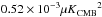$\mathrm{0.52}\mathrm{\times }{\mathrm{10}}^{-3}{\mathit{\mu K}}_{\mathrm{CMB}}^{\mathrm{2}}$ at 150GHz, consistent with the results presented in TableA1 of Abitbol et al. (2016) over the BICEP2 patch (1.3% of the cleanest sky region). Because our dust simulations are noiseless, we can determine the amplitude of the EB spectrum with relatively small error bars. This non-zero dust EB spectrum towards the SGC34 region can produce a spurious B-mode signal, if not taken into account in the self-calibrated telescope polarization angle (Abitbol et al. 2016). Comparing our result with Abitbol et al. (2016) indicates that the amplitude of spurious B-mode signal is negligible at ν ≤ 150GHz, but becomes important at dust frequency channels ν > 217GHz.

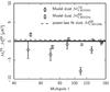Fig. 9 Predicted dust model power spectra ${\mathrm{ℳ}}_{\mathit{\ell }}^{\mathit{TB}}$ (diamonds) and ${\mathrm{ℳ}}_{\mathit{\ell }}^{\mathit{EB}}$ (squares) over SGC34 computed using 100 noiseless Monte-Carlo dust realizations. Dashed curve gives a power-law fit to ${\mathrm{ℳ}}_{\mathit{\ell }}^{\mathit{EB}}$ (see Sect.6.1).

On the other hand, the mean model dust ${\mathrm{ℳ}}_{\mathit{\ell }}^{\mathit{TB}}$ spectrum is mostly negative, but consistent with zero within the 3σ error bar for each multipole bin except for ℓ = 110. 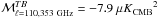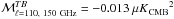The amplitude ${\mathrm{ℳ}}_{\mathit{\ell }\mathrm{=}\mathrm{110}\mathit{,}\mathrm{353}\mathrm{GHz}}^{\mathit{TB}}\mathrm{=}\mathrm{-}\mathrm{7.9}{{\mathit{\mu K}}_{\mathrm{CMB}}}^{\mathrm{2}}$ (or ${\mathrm{ℳ}}_{\mathit{\ell }\mathrm{=}\mathrm{110}\mathit{,}\mathrm{150}\mathrm{GHz}}^{\mathit{TB}}\mathrm{=}\mathrm{-}\mathrm{0.013}{{\mathit{\mu K}}_{\mathrm{CMB}}}^{\mathrm{2}}$ is consistent with the Abitbol et al. (2016) value over the BICEP2 patch (1.3% of the cleanest sky region). The origin of the negative ${\mathrm{ℳ}}_{\mathit{\ell }}^{\mathit{TB}}$ at ℓ = 110 is currently unknown. However, the significance of the negative ${\mathrm{ℳ}}_{\mathit{\ell }}^{\mathit{TB}}$ amplitude goes down with the choice of binning Δℓ> 30. It would be interesting to check our predicted model dust ${\mathrm{ℳ}}_{\mathit{\ell }}^{\mathit{EB}}$ and ${\mathrm{ℳ}}_{\mathit{\ell }}^{\mathit{TB}}$ spectra with the upcoming BICEP2 dust power spectra at 220 GHz.

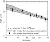Fig. 10 Comparison of the cosmic variance of the dust model ${\mathrm{𝒟}}_{\mathit{\ell }}^{\mathit{BB}}$power spectrum with the one derived from pure Gaussian dust simulations. The statistical variance at low multipoles (ℓ< 80) results from the fixed mean direction of the large-scale GMF (see Sect.6.2).

6.2. Statistical variance of the dust model

In the analysis in BICEP2/Keck Array and Planck Collaborations (2015), Gaussian random realizations of the dust sky are simulated with a spatial power law ℳ_ℓ ∝ ℓ^-0.42 at 353GHz (and scaled to other microwave frequencies using a MBB spectrum with β_d = 1.59 and T_d = 19.6K). In contrast to that Gaussian dust model, our dust model produces non-Gaussianity because it is based on the GASS H I data. Here we test to what degree the statistical variance of the new dust simulations is compatible with the pure Gaussian model approximation.

For this test we proceed as in Sect.5.4 by estimating the mean dust ${\mathrm{ℳ}}_{\mathit{\ell }}^{\mathit{BB}}$ power spectrum at 353GHz over the multipole range 40 < ℓ < 160 and the 1σ standard deviations from 100, in this case noiseless, dust sky realizations over SGC34. These dust model results are shown in Fig.10 as black points, with a power-law fit as the dashed line. Then we assume the hypothesis of Gaussian and statistical isotropy and simulate 100 Gaussian dust sky realizations. The 1σ error range for the BB power from these Gaussian dust realizations is shown as the shaded region in Fig.10.

Comparing these results, our dust simulation band powers shown by the black symbols have less statistical variance at low multipoles ℓ < 80 compared to the variance from the Gaussian sky simulations. This reflects the fact that the model is not constrained exclusively by the dust polarization power spectra. In our dust model, the mean GMF orientation is fixed and the polarization angle of the CNM layer is determined by the GASS H I data. However, at high multipoles ℓ > 80, the effect of B_turb starts dominating over B_ord, leading to a statistical variance that is comparable to or higher than that from the Gaussian sky simulations.

In summary, our dust model predicts smaller statistical variance at multipoles ℓ < 80 compared to the Gaussian dust approximation. Such an effect in the variance is not seen in the Vansyngel et al. (2017) dust model over the same multipole range for the LR regions defined in Planck Collaboration Int.XXX (2016). This is because the amplitudes of the dust polarization power in the Vansyngel et al. (2017) analysis are dominated by the brightest sky areas within these larger regions, whereas by its selection criteria the SGC34 region is more homogeneous.

7. Astrophysical interpretation

In this section we present an astrophysical interpretation of our dust modelling results.

In our analysis the alignment of the CNM structures with B_POS sets the spectral index of the B_turb power spectrum, ${\mathit{\alpha }}_{\mathrm{M}}^{\mathrm{c}}\mathrm{=}\mathrm{-}\mathrm{2.4}$. The Vansyngel et al. (2017) parametric dust model reports α_M = −2.5 for each polarization layer using the CIB-corrected 353 GHz GNILC dust map (Planck Collaboration Int. XLVIII 2016). These two complementary analyses show that the spectral index of the B_turb power spectrum is very close to the slope of the polarized dust power spectra (${\mathrm{𝒟}}_{\mathit{\ell }}^{\mathit{EE}}$, ${\mathrm{𝒟}}_{\mathit{\ell }}^{\mathit{BB}}$, and ${\mathrm{𝒟}}_{\mathit{\ell }}^{\mathit{TE}}$).

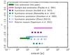Fig. 11 Summary of the observed spectral indices of the power spectrum as a function of length scales (in pc), from dust polarization (solid), synchrotron emission (dashed), synchrotron polarization (dashed-dot), and rotation measures (dotted). See Sect.7 for a detailed description.

Our value of the spectral index α_M is significantly higher (the spectrum is less steep) than the value of −11/3 from the Kolmogorov spectrum. In Fig.11, we compare our result with the spectral indices obtained in earlier studies using starlight polarization (Fosalba et al. 2002), synchrotron emission (Iacobelli et al. 2013; Remazeilles et al. 2015), synchrotron polarization (Haverkorn et al. 2003; Planck Collaboration X 2016), and rotation measures (Oppermann et al. 2012). For each data set we convert the ℓ range to physical sizes. We used a scale-height of 1kpc for the warm ionized medium and the synchrotron emission. For the study of SGC34 here, the maximum distance of the dust emitting layer is L_max = 100−200pc, a range between estimates of the typical distance to the local bubble (Lallement et al. 2014) and of the dust emission scale height (Drimmel & Spergel 2001). All of the values are larger than the spectral index of the Kolmogorov spectrum. In several papers this is explained by introducing an outer scale of turbulence close to the measured physical sizes. However, the current data do not show a consistent systematic trend of spectra steepening towards smaller sizes. Such a trend might be difficult to see combining different tracers of the magnetic field. For dust polarization, we fit the Planck observations over the multipole range 40 < ℓ < 160, which corresponds to physical scales of 2−15pc on the sky. At larger scales, the spectral index from starlight dust polarization (interstellar polarization) is flatter. If this interpretation is correct, then we expect to see further flattening of the B_turb power spectrum at low multipoles (see Fig.20 of Planck Collaboration Int. XLVI 2016). Such flattening, which we neglected in this analysis, could possibly account for the slight differences in the histograms of p² and ψ^R between the Planck data and the dust model (Figs.2 and3).

With our modelling assumption of the same dust alignment parameter (R; see Sect.4.1) for each HI component, we find that the value of ${\mathit{f}}_{\mathrm{M}}^{\mathrm{c}}$ is significantly larger than the value of ${\mathit{f}}_{\mathrm{M}}^{\mathrm{u}\mathit{/}\mathrm{w}}$. The size of ${\mathit{f}}_{\mathrm{M}}^{\mathrm{c}}$ follows from the statistics of the H I CNM map because we assume that B_POS is aligned with CNM structures (Sect.5.1). From ${\mathit{f}}_{\mathrm{M}}^{\mathrm{c}}\mathrm{=}\mathrm{0.4}$, the value of ${\mathit{f}}_{\mathrm{M}}^{\mathrm{u}\mathit{/}\mathrm{w}}$ (0.1) is set by the amplitudes of the observed polarization power spectra (Sect.5.2). Through a consistency check we find that the dispersion of ${\mathit{\psi }}_{\mathrm{m}}^{\mathrm{R}}$ depends on the ${\mathit{f}}_{\mathrm{M}}^{\mathrm{u}\mathit{/}\mathrm{w}}$ value. If we increase the size of ${\mathit{f}}_{\mathrm{M}}^{\mathrm{u}\mathit{/}\mathrm{w}}$, the dispersion of ${\mathit{\psi }}_{\mathrm{m}}^{\mathrm{R}}$ becomes larger than the observed dispersion of ${\mathit{\psi }}_{\mathrm{d}}^{\mathrm{R}}$. Thus our modelling indicates that the CNM component is more turbulent than the UNM/WNM components. This is the first time that this behaviour has been observed in the Planck polarization data. Kalberla et al. (2016) and Heiles & Troland (2003) have shown that the CNM has the largest sonic Mach number. If both the sound and Alfvén speed change by a same factor (≃10) between the CNM and WNM, we also expect a higher Alfvénic Mach number for the CNM than the WNM component (Hennebelle & Passot 2006). This would fit with the larger f_M value in the CNM.

Alternatively, the lower value of f_M for the WNMcomponent could result from our modelling that reduces the LOS integration to a small number of discrete layers. Planck Collaboration Int. XLIV (2016) argued that the number of layers (N_layers) is related to the multiphase structure of the ISM and to the correlation length of the GMF. For the CNM, dust polarization traces the GMF at discrete locations along the LOS. For the WNM, dust polarization samples the variations of the GMF orientation along the LOS. For that ISMphase, N_layers is coming from the correlation length of the GMF that depends on the spectral index of the B_turb power spectrum. For a typical value of α_M = −2.4, the value of N_layers is 6 (Planck Collaboration Int. XLIV 2016). If that reasoning applies, our value of ${\mathit{f}}_{\mathrm{M}}^{\mathrm{w}}$ is effectively a factor $\sqrt{{\mathit{N}}_{\mathrm{layers}}}$ smaller than the true value. The same argument might hold for the UNM component too.

Various alignment mechanisms, such as paramagnetic, mechanical, and radiative torques, have been proposed to explain the efficiency of the alignment of dust grains with respect to the magnetic field (see Lazarian 2003; Andersson et al. 2015, for a review). Draine & Weingartner (1996, 1997) argued that the radiative torques mechanism is the dominant process in the diffuse ISM. We have assumed that the degree of grain alignment and the dust polarization properties are the same in all ISM phases, but they might differ. We investigated this possibility explicitly in our model by keeping fixed p_dust and ${\mathit{f}}_{\mathrm{M}}^{\mathrm{u}\mathit{/}\mathrm{w}}\mathrm{=}\mathrm{0.4}$ and varying the alignment parameter in the cold phase(R_c) and warm phase (R_w). If we lower R_w compared to R_c, the dispersion of ${\mathit{\psi }}_{\mathrm{m}}^{\mathrm{R}}$ becomes broader than the best-fit model presented in this paper. While a lower value R_c compared to R_w provides a better fit to the dispersion of ${\mathit{\psi }}_{\mathrm{d}}^{\mathrm{R}}$, such a model does not reproduce the E−B asymmetry in the power spectrum amplitudes. In summary, within our modelling framework with three H I layers, changes in the (relative) degree of alignment cannot account for the lower value of ${\mathit{f}}_{\mathrm{M}}^{\mathrm{u}\mathit{/}\mathrm{w}}$.

Our values of ${\mathit{f}}_{\mathrm{M}}^{\mathrm{c}}$ and ${\mathit{f}}_{\mathrm{M}}^{\mathrm{u}\mathit{/}\mathrm{w}}$ are lower than the one reported by Planck Collaboration Int. XLIV (2016) and Vansyngel et al. (2017). This difference follows from the model assumptions. We account for the multiphase structure of the ISM and find ${\mathit{f}}_{\mathrm{M}}^{\mathrm{c}}\mathit{>}{\mathit{f}}_{\mathrm{M}}^{\mathrm{u}\mathit{/}\mathrm{w}}$, while Planck Collaboration Int. XLIV (2016) and Vansyngel et al. (2017) keep the same dust total intensity map and f_M value for all of the polarization layers. As discussed in Planck Collaboration Int. XLIV (2016), the best fit values of f_M and p₀ increase with N_layers. In our model, the turbulence is most important in the CNM layer and our value of ${\mathit{f}}_{\mathrm{M}}^{\mathrm{c}}\mathrm{=}\mathrm{0.4}$ is in agreement with the best fit value in Planck Collaboration Int. XLIV (2016) for their one layer model. We also note that our ${\mathit{f}}_{\mathrm{M}}^{\mathrm{c}}$ value applies to the SGC34 region, which by definition is a low column density region (N_{H i} ≤ 2.7 × 10²⁰ cm^-2). Our data analysis suggests that the ${\mathit{f}}_{\mathrm{M}}^{\mathrm{c}}$ value might be higher for the whole SGC region. In our model, we put the mean large-scale GMF in both the UNM and WNM components, thus affecting both ψ^u and ψ^w. This feature of the model can be investigated with numerical simulations. Using a simulation of supernova-driven turbulence in the multiphase ISM, Evirgen et al. (2017) suggest that the mean field might reside preferentially in the WNM.

8. Discussion and summary

We have constructed a phenomenological dust model based on the publicly available GASS H I data and an astrophysically motivated description of the large-scale and turbulent Galactic magnetic field. The two main ingredients of the model are: (1)fluctuations in the GMF orientation along the LOS and (2)a perfect alignment of the CNM structures and B_POS. We model the resulting LOS depolarization by replacing the integration along the LOS by the sum of three distinct components that represent distinct phases of the diffuse neutral atomic ISM. By adjusting a set of nine model parameters suitably, we are able to reproduce the observed statistical properties of the dust polarization in a selected region of low column density (N_{H i} ≤ 2.7 × 10²⁰ cm^-2) that comprises 34% of the southern Galactic cap (SGC34). This dust model is valid only over SGC34.

Unlike PSM dust templates, this dust model is not noise-limited in low column density regions and can be used to predict the average dust polarization at any sky position over the selected region SGC34 at any frequency. This new dust model should be useful for simulating realistic polarized dust skies, testing the accuracy of component separation methods, and studying non-Gaussianity.

Recently, Tassis & Pavlidou (2015) and Poh & Dodelson (2016) showed that multiple dust components along the LOS with different temperatures (in general SEDs) and polarization angles lead to frequency decorrelation in both amplitude and polarization direction. Our dust modelling framework allows us to introduce frequency decorrelation of the dust polarization readily by adopting different dust SEDs for the three H I components and then extrapolating the dust model to other microwave frequencies. With the current Planck sensitivity the current constraint on the dust frequency decorrelation is only marginal at high Galactic latitude (Planck Collaboration Int. L 2017). Although we could use the dust model to explore the frequency decorrelation of the polarized dust emission, this is beyond the scope of this paper.

The main results of the paper are summarized below.

• The observed distributions of p² and ψ over SGC34 can be accounted for by a model with three ISM components: CNM, WNM, and UNM. Each ISM phase has different density structures and different orientations of the turbulent component of the GMF.

• The slopes of ${\mathrm{𝒟}}_{\mathit{\ell }}^{\mathit{EE}}$, ${\mathrm{𝒟}}_{\mathit{\ell }}^{\mathit{BB}}$, and ${\mathrm{𝒟}}_{\mathit{\ell }}^{\mathit{TE}}$ angular power spectra over the multipole range 40 < ℓ < 160 are represented well with the same power-law exponent, which is close to the spectral index of the turbulent magnetic field, α_M = −2.4.

• The positive ${\mathrm{𝒟}}_{\mathit{\ell }}^{\mathit{TE}}$ correlation and E-B power asymmetry over SGC34 can be accounted for by the alignment of the CNM structures with B_POS.

• The E-B power asymmetry for small sky patches depends on the fraction of the total dust emission in the CNM, UNM, and WNM phases. We expect to find the ratio ${\mathrm{𝒟}}_{\mathit{\ell }}^{\mathit{BB}}$/${\mathrm{𝒟}}_{\mathit{\ell }}^{\mathit{EE}}$ close to 1 where the UNM/WNM structures dominate over the CNM structures.

Acknowledgments

The research leading to these results has received funding from the European Research Council grant MISTIC (ERC-267934). Part of the research described in this paper was carried out at the Jet Propulsion Laboratory, California Institute of Technology, under a contract with the National Aeronautics and Space Administration. U.H. acknowledges the support by the Estonian Research Council grant IUT26-2, and by the European Regional Development Fund (TK133). The Parkes Radio Telescope is part of the Australia Telescope, which is funded by the Commonwealth of Australia for operation as a National Facility managed by CSIRO. Some of the results in this paper have been derived using the HEALPix package. Finally, we acknowledge the use of Planck data available from Planck Legacy Archive (http://www.cosmos.esa.int/web/planck/pla).

References

All Tables

All Figures

Fig. 1 NHi maps of the three Gaussian-based HI phases: CNM (top left), UNM (top right), and WNM (bottom left) over the portion of the southern Galactic cap (b ≤ −30°) covered by the GASS HI survey, at 1° resolution. Coloured region corresponds to the selected region SGC34 (bottom right). Orthographic projection in Galactic coordinates: latitudes and longitudes marked by lines and circles respectively.

In the text

Fig. 2 Normalized histograms of p2 over SGC34 at 353GHz. Planck data, ${\mathit{p}}_{\mathrm{d}}^{\mathrm{2}}$, blue inverted-triangles, with 1σerror bars as described in text. The pixel density on the y-axis is the number of pixels in each bin of p2 divided by the total number of pixels over SGC34. Dust model, ${\mathit{p}}_{\mathrm{m}}^{\mathrm{2}}$, black circles connected by line, with 1σ error bars computed from 100Monte-Carlo realizations. The vertical dashed line corresponds to the parameter p0 = 18.5% (${\mathit{p}}_{\mathrm{0}}^{\mathrm{2}}\mathrm{=}\mathrm{0.034}$) of this dust model.

In the text

	Fig. 3 Similar to Fig.2, but for normalized histograms of ψR, the polarization angle relative to the local polarization angle of the large-scale GMF. The vertical dashed line corresponds to a model in which the turbulence is absent (Bturb = 0 so that ψR = 0°).
In the text

Fig. 4 Left column: Planck 353GHz ${\mathrm{𝒟}}_{\mathit{\ell }}^{\mathit{EE}}$ (top row), ${\mathrm{𝒟}}_{\mathit{\ell }}^{\mathit{BB}}$ (middle row), and ${\mathrm{𝒟}}_{\mathit{\ell }}^{\mathit{TE}}$ (bottom row) power spectra in units of ${\mathit{\mu K}}_{\mathrm{CMB}}^{\mathrm{2}}$ computed over SGC34 using the subsets of the Planck data. See text calculation of 1σ error bars. The best-fit power law assuming exponent −2.3 is plotted for each power spectrum (dashed blue line). For comparison, we also show the Planck 2015 best-fit ΛCDM expectation curves for the CMB signal (Planck Collaboration XIII 2016), with the TE expectation shown as dashed where it is negative. Extrapolations of the dust power spectra to 150GHz (see text) are plotted as dashed red lines. Right column: similar to left panels, but for the dust model (Sect.5.4).

In the text

Fig. 5 Mean power spectra of cos2γ (top panel) and cos2ψ (bottom panel) over SGC34 for a set of αM and fM parameters in the multipole range 40 <ℓ< 160. The 1σ error bars are computed from the standard deviations of the 100Monte-Carlo realizations of the dust model. The alignment of the CNM structures with BPOS (see Sect.5.1 for details) constrains the value of ${\mathit{\alpha }}_{\mathrm{M}}^{\mathrm{c}}$ and ${\mathit{f}}_{\mathrm{M}}^{\mathrm{c}}$ for the CNM component.

In the text

	Fig. 6 Correlation of the Planck 353GHz dust intensity map and the dust model StokesI map. The dashed line is the best-fit relation.
In the text

	Fig. 7 Best-fit power law dust model TT power spectra at 353GHz (black dashed line) and extrapolated dust power spectra at 150GHz (red dashed line) as computed over SGC34. For comparison, we also show the Planck 2015 best-fit ΛCDM expectation curves of the CMB signal.
In the text

Fig. 8 Left column: orthographic projections of the Planck 353GHz D353 (StokesI) map (top row) and the square of the polarization intensity P2 (bottom row), at 1° resolution over the southern Galactic cap covered by the GASS H I survey, with the selected region SGC34 outlined by a black contour. The same coordinate system is used as in Fig.1. Right column: similar to left panels, but for a realization of the 353GHz dust model. Judged visually, the dust model is able to reproduce roughly the observed dust polarization sky over SGC34, and indeed over the entire field shown.

In the text

	Fig. 9 Predicted dust model power spectra ${\mathrm{ℳ}}_{\mathit{\ell }}^{\mathit{TB}}$ (diamonds) and ${\mathrm{ℳ}}_{\mathit{\ell }}^{\mathit{EB}}$ (squares) over SGC34 computed using 100 noiseless Monte-Carlo dust realizations. Dashed curve gives a power-law fit to ${\mathrm{ℳ}}_{\mathit{\ell }}^{\mathit{EB}}$ (see Sect.6.1).
In the text

	Fig. 10 Comparison of the cosmic variance of the dust model ${\mathrm{𝒟}}_{\mathit{\ell }}^{\mathit{BB}}$power spectrum with the one derived from pure Gaussian dust simulations. The statistical variance at low multipoles (ℓ< 80) results from the fixed mean direction of the large-scale GMF (see Sect.6.2).
In the text

	Fig. 11 Summary of the observed spectral indices of the power spectrum as a function of length scales (in pc), from dust polarization (solid), synchrotron emission (dashed), synchrotron polarization (dashed-dot), and rotation measures (dotted). See Sect.7 for a detailed description.
In the text

References

- Abbott, L.F., & Wise, M.B. 1984, Nucl. Phys. B, 244, 541 [NASA ADS] [CrossRef] [MathSciNet] [Google Scholar]
- Abitbol, M.H., Hill, J.C., & Johnson, B.R. 2016, MNRAS, 457, 1796 [NASA ADS] [CrossRef] [Google Scholar]
- Andersson, B.-G., Lazarian, A., & Vaillancourt, J.E. 2015, ARA&A, 53, 501 [NASA ADS] [CrossRef] [Google Scholar]
- Audit, E., & Hennebelle, P. 2005, A&A, 433, 1 [NASA ADS] [CrossRef] [EDP Sciences] [Google Scholar]
- Benson, B.A., Ade, P.A.R., Ahmed, Z., et al. 2014, in Millimeter, Submillimeter, and Far-Infrared Detectors and Instrumentation for Astronomy VII, Proc.SPIE, 9153, 91531P [Google Scholar]
- Betoule, M., Pierpaoli, E., Delabrouille, J., Le Jeune, M., & Cardoso, J.-F. 2009, A&A, 503, 691 [NASA ADS] [CrossRef] [EDP Sciences] [Google Scholar]
- BICEP2/Keck Array and Planck Collaborations 2015, Phys. Rev. Lett., 114, 101301 [NASA ADS] [CrossRef] [PubMed] [Google Scholar]
- BICEP2 and Keck Array Collaboration, Ade, P.A.R., Ahmed, Z., et al. 2016, Phys. Rev. Lett., 116, 031302 [NASA ADS] [CrossRef] [PubMed] [Google Scholar]
- Boulanger, F., Abergel, A., Bernard, J.-P., et al. 1996, A&A, 312, 256 [NASA ADS] [Google Scholar]
- Bowyer, J., Jaffe, A.H., & Novikov, D.I. 2011, MasQU: Finite Differences on Masked Irregular StokesQ, U Grids, Astrophysics Source Code Library [Google Scholar]
- Caldwell, R.R., Hirata, C., & Kamionkowski, M. 2017, ApJ, 839, 91 [NASA ADS] [CrossRef] [Google Scholar]
- Cho, J., & Lazarian, A. 2002, ApJ, 575, L63 [NASA ADS] [CrossRef] [Google Scholar]
- Cho, J., & Lazarian, A. 2010, ApJ, 720, 1181 [NASA ADS] [CrossRef] [Google Scholar]
- Chon, G., Challinor, A., Prunet, S., Hivon, E., & Szapudi, I. 2004, MNRAS, 350, 914 [NASA ADS] [CrossRef] [Google Scholar]
- Clark, S.E., Peek, J.E.G., & Putman, M.E. 2014, ApJ, 789, 82 [NASA ADS] [CrossRef] [Google Scholar]
- Clark, S.E., Hill, J.C., Peek, J.E.G., Putman, M.E., & Babler, B.L. 2015, Phys. Rev. Lett., 115, 241302 [NASA ADS] [CrossRef] [Google Scholar]
- Crill, B.P., Ade, P.A.R., Battistelli, E.S., et al. 2008, in Space Telescopes and Instrumentation 2008: Optical, Infrared, and Millimeter, Proc.SPIE, 7010, 70102 [Google Scholar]
- Delabrouille, J., Betoule, M., Melin, J.-B., et al. 2013, A&A, 553, A96 [NASA ADS] [CrossRef] [EDP Sciences] [Google Scholar]
- Draine, B.T., & Weingartner, J.C. 1996, ApJ, 470, 551 [NASA ADS] [CrossRef] [Google Scholar]
- Draine, B.T., & Weingartner, J.C. 1997, ApJ, 480, 633 [NASA ADS] [CrossRef] [Google Scholar]
- Drimmel, R., & Spergel, D.N. 2001, ApJ, 556, 181 [NASA ADS] [CrossRef] [Google Scholar]
- Essinger-Hileman, T., Appel, J.W., Beall, J.A., et al. 2010, ArXiv e-prints [arXiv:1008.3915] [Google Scholar]
- Essinger-Hileman, T., Ali, A., Amiri, M., et al. 2014, in Millimeter, Submillimeter, and Far-Infrared Detectors and Instrumentation for Astronomy VII, Proc.SPIE, 9153, 91531 [Google Scholar]
- Evirgen, C.C., Gent, F.A., Shukurov, A., Fletcher, A., & Bushby, P. 2017, MNRAS, 464, L105 [NASA ADS] [CrossRef] [Google Scholar]
- Fabbri, R., & Pollock, M.D. 1983, Phys. Lett. B, 125, 445 [NASA ADS] [CrossRef] [Google Scholar]
- Fauvet, L., Macías-Pérez, J.F., Jaffe, T.R., et al. 2012, A&A, 540, A122 [NASA ADS] [CrossRef] [EDP Sciences] [Google Scholar]
- Fosalba, P., Lazarian, A., Prunet, S., & Tauber, J.A. 2002, ApJ, 564, 762 [NASA ADS] [CrossRef] [Google Scholar]
- Gillmon, K., Shull, J.M., Tumlinson, J., & Danforth, C. 2006, ApJ, 636, 891 [NASA ADS] [CrossRef] [Google Scholar]
- Górski, K.M., Hivon, E., Banday, A.J., et al. 2005, ApJ, 622, 759 [NASA ADS] [CrossRef] [Google Scholar]
- Grain, J., Tristram, M., & Stompor, R. 2009, Phys.Rev.D, 79, 123515 [NASA ADS] [CrossRef] [Google Scholar]
- Green, G.M., Schlafly, E.F., Finkbeiner, D.P., et al. 2015, ApJ, 810, 25 [NASA ADS] [CrossRef] [Google Scholar]
- Haud, U. 2013, A&A, 552, A108 [NASA ADS] [CrossRef] [EDP Sciences] [Google Scholar]
- Haud, U., & Kalberla, P.M.W. 2007, A&A, 466, 555 [NASA ADS] [CrossRef] [EDP Sciences] [Google Scholar]
- Haverkorn, M., Katgert, P., & de Bruyn, A.G. 2003, A&A, 403, 1045 [NASA ADS] [CrossRef] [EDP Sciences] [Google Scholar]
- Heiles, C., & Troland, T.H. 2003, ApJ, 586, 1067 [NASA ADS] [CrossRef] [Google Scholar]
- Heiles, C., & Troland, T.H. 2005, ApJ, 624, 773 [NASA ADS] [CrossRef] [Google Scholar]
- Henderson, S.W., Allison, R., Austermann, J., et al. 2016, J. Low Temperature Phys., 184, 772 [NASA ADS] [CrossRef] [Google Scholar]
- Hennebelle, P. 2013, A&A, 556, A153 [NASA ADS] [CrossRef] [EDP Sciences] [Google Scholar]
- Hennebelle, P., & Iffrig, O. 2014, A&A, 570, A81 [NASA ADS] [CrossRef] [EDP Sciences] [Google Scholar]
- Hennebelle, P., & Passot, T. 2006, A&A, 448, 1083 [NASA ADS] [CrossRef] [EDP Sciences] [Google Scholar]
- Iacobelli, M., Haverkorn, M., Orrú, E., et al. 2013, A&A, 558, A72 [NASA ADS] [CrossRef] [EDP Sciences] [Google Scholar]
- Inoue, T., & Inutsuka, S.-I. 2016, ApJ, 833, 10 [NASA ADS] [CrossRef] [Google Scholar]
- Jaffe, T.R., Leahy, J.P., Banday, A.J., et al. 2010, MNRAS, 401, 1013 [NASA ADS] [CrossRef] [Google Scholar]
- Kalberla, P.M.W., & Haud, U. 2015, A&A, 578, A78 [NASA ADS] [CrossRef] [EDP Sciences] [Google Scholar]
- Kalberla, P.M.W., McClure-Griffiths, N.M., Pisano, D.J., et al. 2010, A&A, 521, A17 [NASA ADS] [CrossRef] [EDP Sciences] [Google Scholar]
- Kalberla, P.M.W., Kerp, J., Haud, U., et al. 2016, ApJ, 821, 117 [NASA ADS] [CrossRef] [Google Scholar]
- Kermish, Z.D., Ade, P., Anthony, A., et al. 2012, in Millimeter, Submillimeter, and Far-Infrared Detectors and Instrumentation for Astronomy VI, Proc. SPIE, 8452, 84521 [Google Scholar]
- Lallement, R., Vergely, J.-L., Valette, B., et al. 2014, A&A, 561, A91 [NASA ADS] [CrossRef] [EDP Sciences] [Google Scholar]
- Lazarian, A. 2003, J.Quant.Spec.Radiat.Transf., 79, 881 [NASA ADS] [CrossRef] [Google Scholar]
- Lazarian, A. 2008, ArXiv e-prints [arXiv:astro-ph/0811.1020] [Google Scholar]
- Martin, P.G., Blagrave, K.P.M., Lockman, F.J., et al. 2015, ApJ, 809, 153 [NASA ADS] [CrossRef] [Google Scholar]
- McClure-Griffiths, N.M., Pisano, D.J., Calabretta, M.R., et al. 2009, ApJS, 181, 398 [NASA ADS] [CrossRef] [Google Scholar]
- Montier, L., Plaszczynski, S., Levrier, F., et al. 2015, A&A, 574, A136 [NASA ADS] [CrossRef] [EDP Sciences] [Google Scholar]
- Nidever, D.L., Majewski, S.R., Butler Burton, W., & Nigra, L. 2010, ApJ, 723, 1618 [NASA ADS] [CrossRef] [Google Scholar]
- O’Dea, D.T., Clark, C.N., Contaldi, C.R., & MacTavish, C.J. 2012, MNRAS, 419, 1795 [NASA ADS] [CrossRef] [Google Scholar]
- Ogburn, R.W., Ade, P.A.R., Aikin, R.W., et al. 2012, in Millimeter, Submillimeter, and Far-Infrared Detectors and Instrumentation for Astronomy VI, Proc.SPIE, 8452, 84521 [Google Scholar]
- Oppermann, N., Junklewitz, H., Robbers, G., et al. 2012, A&A, 542, A93 [NASA ADS] [CrossRef] [EDP Sciences] [Google Scholar]
- Peek, J.E.G., Heiles, C., Douglas, K.A., et al. 2011, ApJS, 194, 20 [NASA ADS] [CrossRef] [Google Scholar]
- Planck Collaboration VI. 2014, A&A, 571, A6 [NASA ADS] [CrossRef] [EDP Sciences] [Google Scholar]
- Planck Collaboration XI. 2014, A&A, 571, A11 [NASA ADS] [CrossRef] [EDP Sciences] [Google Scholar]
- Planck Collaboration XVI. 2014, A&A, 571, A16 [NASA ADS] [CrossRef] [EDP Sciences] [Google Scholar]
- Planck Collaboration I. 2016, A&A, 594, A1 [NASA ADS] [CrossRef] [EDP Sciences] [Google Scholar]
- Planck Collaboration VIII. 2016, A&A, 594, A8 [NASA ADS] [CrossRef] [EDP Sciences] [Google Scholar]
- Planck Collaboration X. 2016, A&A, 594, A10 [NASA ADS] [CrossRef] [EDP Sciences] [Google Scholar]
- Planck Collaboration XII. 2016, A&A, 594, A12 [NASA ADS] [CrossRef] [EDP Sciences] [Google Scholar]
- Planck Collaboration XIII. 2016, A&A, 594, A13 [NASA ADS] [CrossRef] [EDP Sciences] [Google Scholar]
- Planck Collaboration XVI. 2016, A&A, 594, A16 [NASA ADS] [CrossRef] [EDP Sciences] [Google Scholar]
- Planck Collaboration Int. XVII. 2014, A&A, 566, A55 [NASA ADS] [CrossRef] [EDP Sciences] [Google Scholar]
- Planck Collaboration Int. XIX. 2015, A&A, 576, A104 [NASA ADS] [CrossRef] [EDP Sciences] [Google Scholar]
- Planck Collaboration Int. XX. 2015, A&A, 576, A105 [NASA ADS] [CrossRef] [EDP Sciences] [Google Scholar]
- Planck Collaboration Int. XXII. 2015, A&A, 576, A107 [NASA ADS] [CrossRef] [EDP Sciences] [Google Scholar]
- Planck Collaboration Int. XXX. 2016, A&A, 586, A133 [NASA ADS] [CrossRef] [EDP Sciences] [Google Scholar]
- Planck Collaboration Int. XXXII. 2016, A&A, 586, A135 [NASA ADS] [CrossRef] [EDP Sciences] [Google Scholar]
- Planck Collaboration Int. XXXV. 2016, A&A, 586, A138 [NASA ADS] [CrossRef] [EDP Sciences] [Google Scholar]
- Planck Collaboration Int. XXXVIII. 2016, A&A, 586, A141 [NASA ADS] [CrossRef] [EDP Sciences] [Google Scholar]
- Planck Collaboration Int. XLIV. 2016, A&A, 596, A105 [NASA ADS] [CrossRef] [EDP Sciences] [Google Scholar]
- Planck Collaboration Int. XLVI. 2016, A&A, 596, A107 [NASA ADS] [CrossRef] [EDP Sciences] [Google Scholar]
- Planck Collaboration Int. XLVIII. 2016, A&A, 596, A109 [NASA ADS] [CrossRef] [EDP Sciences] [Google Scholar]
- Planck Collaboration Int. L. 2017, A&A, 599, A51 [NASA ADS] [CrossRef] [EDP Sciences] [Google Scholar]
- Poh, J., & Dodelson, S. 2016, ArXiv e-prints [arXiv:1606.08922] [Google Scholar]
- Prunet, S., & Lazarian, A. 1999, in Microwave Foregrounds, eds. A.de Oliveira-Costa, & M.Tegmark, ASP Conf. Ser., 181, 113 [Google Scholar]
- Reichborn-Kjennerud, B., Aboobaker, A.M., Ade, P., et al. 2010, in Millimeter, Submillimeter, and Far-Infrared Detectors and Instrumentation for Astronomy V, Proc.SPIE, 7741, 77411 [Google Scholar]
- Remazeilles, M., Dickinson, C., Banday, A.J., Bigot-Sazy, M.-A., & Ghosh, T. 2015, MNRAS, 451, 4311 [NASA ADS] [CrossRef] [Google Scholar]
- Saury, E., Miville-Deschênes, M.-A., Hennebelle, P., Audit, E., & Schmidt, W. 2014, A&A, 567, A16 [NASA ADS] [CrossRef] [EDP Sciences] [Google Scholar]
- Simmons, J.F.L., & Stewart, B.G. 1985, A&A, 142, 100 [Google Scholar]
- Starobinsky, A.A. 1979, Pisma v Zhurnal Eksperimentalnoi i Teoreticheskoi Fiziki, 30, 719 [NASA ADS] [Google Scholar]
- Suzuki, A., Ade, P., Akiba, Y., et al. 2016, J. Low Temperature Phys., 184, 805 [NASA ADS] [CrossRef] [Google Scholar]
- Tassis, K., & Pavlidou, V. 2015, MNRAS, 451, L90 [NASA ADS] [CrossRef] [Google Scholar]
- Tristram, M., Macías-Pérez, J.F., Renault, C., & Santos, D. 2005, MNRAS, 358, 833 [NASA ADS] [CrossRef] [Google Scholar]
- Vansyngel, F., Boulanger, F., Ghosh, T., et al. 2017, A&A, in press, DOI:10.1051/0004-6361/201629992 [Google Scholar]
- Winkel, B., Kerp, J., Flöer, L., et al. 2016, A&A, 585, A41 [NASA ADS] [CrossRef] [EDP Sciences] [Google Scholar]
- Wolfire, M.G., McKee, C.F., Hollenbach, D., & Tielens, A.G.G.M. 2003, ApJ, 587, 278 [NASA ADS] [CrossRef] [Google Scholar]
- Zaldarriaga, M., & Seljak, U. 1997, Phys.Rev.D, 55, 1830 [NASA ADS] [CrossRef] [Google Scholar]
All Tables
Dust polarization fraction p statistics at 353GHz and the best-fit mean direction of the large-scale GMF over SGC34 using multiple subsets of the Planck data.
Fitted 353GHz dust power spectra of the Planck data and of the dust model over SGC34, for which the mean dust intensity ⟨ D353 ⟩ is 54 ± 3kJysr-1.