| Issue |
A&A
Volume 577, May 2015
|
|
|---|---|---|
| Article Number | A37 | |
| Number of page(s) | 27 | |
| Section | Extragalactic astronomy | |
| DOI | https://doi.org/10.1051/0004-6361/201425302 | |
| Published online | 28 April 2015 | |
Anatomy of the AGN in NGC 5548
II. The spatial, temporal, and physical nature of the outflow from HST/COS Observations⋆
1
Department of Physics, Virginia Tech, Blacksburg, VA
24061, USA
e-mail: This email address is being protected from spambots. You need JavaScript enabled to view it.
2
Space Telescope Science Institute, 3700 San Martin Drive, Baltimore, MD
21218,
USA
3
Department of Physics and Astronomy, The Johns Hopkins
University, Baltimore, MD
21218,
USA
4
SRON Netherlands Institute for Space Research,
Sorbonnelaan 2, 3584 CA
Utrecht, The
Netherlands
5
Leiden Observatory, Leiden University,
Post Office Box 9513,
2300 RA
Leiden, The
Netherlands
6
INAF−IASF Bologna, via Gobetti 101, 40129
Bologna,
Italy
7
Mullard Space Science Laboratory, University College
London, Holmbury St. Mary,
Dorking, Surrey,
RH5 6NT,
UK
8
Univ. Grenoble Alpes, IPAG, 38000
Grenoble,
France
9
CNRS, IPAG, 38000
Grenoble,
France
10
Instituto de Astronomía, Universidad Católica del
Norte, Avenida Angamos 0610,
Casilla 1280, Antofagasta, Chile
11
Department of Physics, University of Oxford,
Keble Road, Oxford, OX1
3RH, UK
12
Department of Physics, Technion-Israel Institute of
Technology, 32000
Haifa,
Israel
13
Dipartimento di Matematica e Fisica, Università degli Studi Roma
Tre, via della Vasca Navale
84, 00146
Roma,
Italy
14
Department of Astronomy, University of Geneva,
16 Ch. d’Ecogia, 1290
Versoix,
Switzerland
15
Cahill Center for Astronomy and Astrophysics, California Institute
of Technology, Pasadena, CA
91125,
USA
16
Université de Toulouse, UPS-OMP, IRAP,
31028
Toulouse,
France
17
CNRS, IRAP, 9
Av. colonel Roche, BP
44346, 31028
Toulouse Cedex 4,
France
18
Max-Planck-Institut für extraterrestrische Physik,
Giessenbachstrasse,
85748
Garching,
Germany
19
Department of Astronomy, The Ohio State University,
140W 18th Avenue, Columbus, OH
43210,
USA
20
Center for Cosmology & AstroParticle Physics, The Ohio State
University, 191 West Woodruff
Avenue, Columbus,
OH
43210,
USA
21
Institute of Astronomy, University of Cambridge,
Madingley Rd, Cambridge, CB3 0HA, UK
22
Astronomisches Institut, Ruhr-Universität Bochum,
Universitätsstraße 150, 44801
Bochum,
Germany
23
INAF/IAPS−
via Fosso del Cavaliere 100,
00133
Roma,
Italy
24
Research Center for Measurement in Advanced Science, Faculty of
Science, Rikkyo University 3-34-1
Nishi-Ikebukuro, Toshima-ku, Tokyo, Japan
Received: 7 November 2014
Accepted: 2 March 2015
Abstract
Context. AGN outflows are thought to influence the evolution of their host galaxies and of super massive black holes. Our deep multiwavelength campaign on NGC 5548 has revealed a new, unusually strong X-ray obscuration, accompanied by broad UV absorption troughs observed for the first time in this object. The X-ray obscuration caused a dramatic decrease in the incident ionizing flux on the outflow that produces the long-studied narrow UV absorption lines in this AGN. The resulting data allowed us to construct a comprehensive physical, spatial, and temporal picture for this enduring AGN wind.
Aims. We aim to determine the distance of the narrow UV outflow components from the central source, their total column-density, and the mechanism responsible for their observed absorption variability.
Methods. We study the UV spectra acquired during the campaign, as well as from four previous epochs (1998−2011). Our main analysis tools are ionic column-density extraction techniques, photoionization models based on the code CLOUDY, and collisional excitation simulations.
Results. A simple model based on a fixed total column-density absorber, reacting to changes in ionizing illumination, matches the very different ionization states seen in five spectroscopic epochs spanning 16 years. The main component of the enduring outflow is situated at 3.5 ± 1.1 pc from the central source, and its distance and number density are similar to those of the narrow-emitting-line region in this object. Three other components are situated between 5−70 pc and two are farther than 100 pc. The wealth of observational constraints and the anti-correlation between the observed X-ray and UV flux in the 2002 and 2013 epochs make our physical model a leading contender for interpreting trough variability data of quasar outflows.
Conclusions. This campaign, in combination with prior UV and X-ray data, yields the first simple model that can explain the physical characteristics and the substantial variability observed in an AGN outflow.
Key words: galaxies: Seyfert
Appendix A is available in electronic form at http://www.aanda.org
© ESO, 2015
1. Introduction
AGN outflows are detected as blueshifted absorption troughs with respect to the object systemic redshift. Such outflows in powerful quasars can expel sufficient gas from their host galaxies to halt star formation, limit their growth, and lead to the co-evolution of the size of the host and the mass of its central super massive black holes (e.g., Ostriker et al. 2010; Hopkins & Elvis 2010; Soker & Meiron 2011; Ciotti et al. 2010; Faucher-Giguère et al. 2012; Borguet et al. 2013; Arav et al. 2013). Therefore, deciphering the properties of AGN outflows is crucial for testing their role in galaxy evolution.
Nearby bright AGN are excellent laboratories for studying these outflows because they yield: a) high-resolution UV data, which allow us to study the outflow kinematics and can yield diagnostics for their distance from the central source; and b) high-quality X-ray spectra that give the physical conditions for the bulk of the outflowing material (e.g., Steenbrugge et al. 2005; Gabel et al. 2005; Arav et al. 2007; Costantini et al. 2007; Kaastra et al. 2012). Thus, such observations are a vital stepping stone for quantifying outflows from the luminous (but distant) quasars, for which high-quality X-ray data are not available.
For these reasons, we embarked on a deep multiwavelength campaign on the prototypical AGN outflow seen in the intensively studied Seyfert 1 galaxy NGC 5548. For the past 16 years, this outflow has shown six kinematic components in the UV band (labeled in descending order of velocity, following Crenshaw et al. 2003), and their associated X-ray warm absorber (WA). We note that there is kinematic correspondence between the six UV components and the deduced WA components (see Sect. 5.1). Our 2013 campaign revealed a new X-ray obscurer accompanied by broad UV absorption (analyzed in Kaastra et al. 2014). The appearance of the obscurer allows us to derive a comprehensive physical picture of the long-term observed outflow, which we report here.
The plan of the paper is as follows. In Sect. 2 we describe the observations and data reduction; in Sect. 3 we analyze the key component of the outflow; in Sect. 4 we discuss the remaining five components; in Sect. 5 we connect the results of the UV analysis with those of the X-ray warm absorber of the same outflow; and in Sect. 6 we compare our results with previous studies, discuss the implication of our results to the variability of AGN outflow troughs in general, and elaborate on the connection between the X-ray obscurer and the persisting outflow; in Sect. 7 we summarize our results.
2. Observations and data reduction
Our 2013 multiwavelength campaign on NGC 5548 included coordinated observations using XMM-Newton, the Hubble Space Telescope (HST), Swift, INTEGRAL and NuSTAR. The overall structure of the campaign was described in Kaastra et al. (2014). A full log of all the observations is given by Mehdipour et al (2014). Here we present a detailed analysis of the UV observations we obtained using the Cosmic Origins Spectrograph (COS) (Green et al. 2012) onboard HST. We obtained five COS observations simultaneously with five of the XMM-Newton observations between 2013 June 22 and 2013 August 01. Each two-orbit observation used gratings G130M and G160M at multiple central wavelength settings and multiple focal-plane positions (FP-POS) to cover the wavelength range from 1132 Å to 1801 Å at a resolving power of ~15 000. Table A.1 lists the observation dates of the individual visits, the exposure times, and the continuum flux measured at 1350 Å in the rest frame, as well as corresponding information for archival HST observations of NGC 5548 that are also used in this analysis. The five observations from June to August 2013 were optimally weighted to produce an average spectrum that we use for our analysis. Kaastra et al. (2014) describe the data reduction process from the calibration of the data to the production of this average spectrum.
The 2013 average HST/COS spectrum with all identified absorption features is shown in Fig. A.1. As described in Kaastra et al. (2014), we modeled the emission from NGC 5548 using a reddened power law (with extinction fixed at E(B − V) = 0.02, Schlafly & Finkbeiner 2011), weak Fe ii emission longward of 1550 Å in the rest frame, broad and narrow emission lines modeled with several Gaussian components, blueshifted broad absorption on all permitted transitions in NGC 5548, and a Galactic damped Lyα absorption line. Using this emission model, we normalized the average spectrum to facilitate our analysis of the narrow intrinsic absorption lines in NGC 5548. Figure 1 shows normalized spectra for absorption lines produced by Si iiiλ1206, Si ivλλ1394,1403, C ivλλ1548,1550, N vλλ1238,1242, and Ly α as a function of rest-frame velocity relative to a systemic redshift of z = 0.017175 (de Vaucouleurs et al. 1991) via the NASA/IPAC extragalactic database (NED).
As shown in Table A.1, high-resolution UV spectra of NGC 5548 using HST cover an additional four epochs stretching back to 1998. We use the calibrated data sets for each of these observations as obtained from the Mikulski Archive for Space Telescopes (MAST) at the Space Telescope Science Institute (STScI). We compare the strengths of the narrow UV absorption troughs for each of these epochs with our new data set from 2013 in Figs. A.2 and A.3.
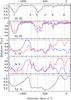 |
Fig. 1 Intrinsic absorption features in the 2013 COS spectrum of NGC 5548. Normalized relative fluxes are plotted as a function of velocity relative to the systemic redshift of z = 0.017175, top to bottom: Si iiiλ1206, Si ivλλ1394,1403, C ivλλ1548,1550, N vλλ1238,1242, and Ly α, as a function of rest-frame velocity. For the doublets the red and blue components are shown in red and blue, respectively. Dotted vertical lines indicate the velocities of the absorption components numbered as in Crenshaw et al. (2003). |
3. Physical and temporal characteristics of component 1
The key for building a coherent picture of the long-seen outflow is component 1: the strongest and highest velocity outflow component (centered at −1160 km s-1). Due to the strong suppression of incident ionizing flux by the obscurer, the 2013 HST/COS data of component 1 show a wealth of absorption troughs from ions never before observed in the NGC 5548 outflow. These data allow us to decipher the physical characteristics of this component. In Sect. 3.1 we use the column-density measurements of P v, P iii, Fe iii, and Si ii as input in photoionization models, and derive the total hydrogen column-density (NH) for component 1, and its ionization parameter (UH). In Sect. 3.2 we use the column-density measurements of C iii* and Si iii* to infer the electron number density (ne), which combined with the value of the incident UH yields a distance (R) between component 1 and the central source. In Sect. 3.3 we construct a simple model based on a fixed total column-density absorber, reacting to changes in ionizing illumination, that matches the very different ionization states seen in five HST high-resolution spectroscopic epochs spanning 16 years.
3.1. Total column-density  and ionization parameter (UH)
In the Appendix we describe the methods we use to derive the ionic column-densities
 from the outflow absorption troughs. Table
A.2 gives the Nion
measurements for all observed troughs of all six outflow components in the five HST epochs
(spanning 16 years) of high-resolution UV spectroscopy. The upper and lower limits were
derived using the apparent optical depth (AOD) method. All the reported measurements were
done using the partial overing (PC) method. We used the power-law (PL) method only on the
C iii* in order to quantify the systematic error due to different measuring
methods (see Sect. 3.2).
from the outflow absorption troughs. Table
A.2 gives the Nion
measurements for all observed troughs of all six outflow components in the five HST epochs
(spanning 16 years) of high-resolution UV spectroscopy. The upper and lower limits were
derived using the apparent optical depth (AOD) method. All the reported measurements were
done using the partial overing (PC) method. We used the power-law (PL) method only on the
C iii* in order to quantify the systematic error due to different measuring
methods (see Sect. 3.2).
The Nion we measure are a result of the ionization structure of the outflowing material, and can be compared to photoionization models to determine the physical characteristics of the absorbing gas. As boundary conditions for the photoionization models, we need to specify the choice of incident spectral energy distribution (SED), and the chemical abundances of the outflowing gas.
We make the simple (and probably over-restrictive) assumption that the shape of the SED emitted from the accretion disk did not change over the 16 years of high-resolution UV spectroscopy. Specifically, we assume that the emitted SED has the same shape it had when we obtained simultaneous X-ray/UV observations in 2002 (the “high” SED in Fig. 2, determined by Steenbrugge et al. 2005). In 2013 the obscurer absorbed much of the soft ionizing photon flux from this SED before it reached component 1. We model the incident SED on component 1 as the “obscured” SED in Fig. 2, and further justify its specific shape in Sect. 3.3 For abundances, we use pure proto-Solar abundances given by Lodders et al. (2009). The influence of the suppressed ionizing continuum on the photoionization solution is also discussed in Sect. 3.3.
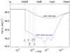 |
Fig. 2 Adopted NGC 5548 SEDs. In black we show the SED for NGC 5548 in 2002 at an unobscured X-ray flux (hereafter “high SED”, from Steenbrugge et al. 2005). In blue we show the SED appropriate to the 2013 epoch, where for the same flux at 1000 Å, the new X-ray obscurer reduced the ionizing flux by a factor of 17 between 1 Ry and 1 keV (obscured SED). The ionization potentials for destruction of some of the prominent observed species are shown by the vertical lines. |
With the choice of SED and chemical abundances, two main parameters govern the
photoionization structure of the absorber: the total hydrogen column-density
 and the ionization parameter
 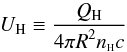 (1)where QH is the rate
of hydrogen-ionizing photons emitted by the object, c is the speed of light,
R is the
distance from the central source to the absorber and nH is the total
hydrogen number density. We model the photoionization structure and predict the resulting
ionic column densities by self-consistently solving the ionization and thermal balance
equations with version 13.01 of the spectral synthesis code CLOUDY, last described in
Ferland et al. (2013). We assume a plane-parallel
geometry for a gas of constant nH.
(1)where QH is the rate
of hydrogen-ionizing photons emitted by the object, c is the speed of light,
R is the
distance from the central source to the absorber and nH is the total
hydrogen number density. We model the photoionization structure and predict the resulting
ionic column densities by self-consistently solving the ionization and thermal balance
equations with version 13.01 of the spectral synthesis code CLOUDY, last described in
Ferland et al. (2013). We assume a plane-parallel
geometry for a gas of constant nH.
To find the pair of  that best predicts the set of observed
column-densities, we vary UH and NH in 0.1 dex
steps to generate a grid of models (following the same approach described in Borguet et al. 2012b) and perform a minimization of the
function
that best predicts the set of observed
column-densities, we vary UH and NH in 0.1 dex
steps to generate a grid of models (following the same approach described in Borguet et al. 2012b) and perform a minimization of the
function 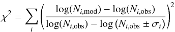 (2)where, for ion i, Ni,obs and
Ni,mod are the observed
and modeled column-densities, respectively, and σi is the error in the
observed column-density. The measurement errors are not symmetric. We use the positive
error (+
σi) when
log (Ni,mod) >
log (Ni,obs) and the
negative error (−σi) when
log (Ni,mod) <
log (Ni,obs).
(2)where, for ion i, Ni,obs and
Ni,mod are the observed
and modeled column-densities, respectively, and σi is the error in the
observed column-density. The measurement errors are not symmetric. We use the positive
error (+
σi) when
log (Ni,mod) >
log (Ni,obs) and the
negative error (−σi) when
log (Ni,mod) <
log (Ni,obs).
The ionization solution for component 1 at the 2013 epoch is shown in Fig. 3. We only show constraints from Nion
measurements, and note that all the lower limits reported in Table 2 are satisfied by this
solution. We find  cm-2, and an ionization parameter
of
cm-2, and an ionization parameter
of 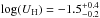 , where the errors are strongly correlated
as illustrated by the 1σχ2 contour.
, where the errors are strongly correlated
as illustrated by the 1σχ2 contour.
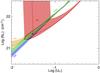 |
Fig. 3 Photoionization phase plot showing the ionization solution for component 1 epoch 2013. We use the obscured SED and assumed proto-solar metalicity (Lodders et al. 2009). Solid lines and associated colored bands represent the locus of UH,NH models, which predict the measured Nion, and their 1σ uncertainties. The black dot is the best solution and is surrounded by a 1σχ2 contour. |
3.2. Number density and distance
 |
Fig. 4 a) Absorption spectrum for the C iii* 1175 Å multiplet. The 2013 COS spectrum shows clear and relatively unblended individual troughs from the J = 2 and J = 0 levels, but no contribution from the J = 1 level that is populated at higher densities (see panel c)). b) Absorption spectrum for the Si iii* 1298 Å multiplet (similar in level structure to the C iii* 1175 Å multiplet). The 2013 COS spectrum shows shallow but highly significant individual troughs from the J = 2 and J = 0 levels, but again no contribution from the J = 1 level that is populated at higher densities. c) C iii* and Si iii* level population ratios, theory and measurements. The computed populations for the J = 2/J = 0 and J = 1/J = 0 are plotted as a function of electron number density for both ions (see text for elaboration). The crosses show the measured ratios for the J = 2/J = 0 ratio of both ions. From the C iii* ratios we infer log (ne) = 4.8 ± 0.1 cm-3, where the error includes both statistical and systematic effects. This value is fully consistent with the one inferred from the Si iii* ratio, where in the case of Si iii* the statistical error is larger since the troughs are much shallower. |
As shown in Fig. 4, we detect absorption troughs from the C iii* 1175 Å multiplet, arising from the metastable 3Pj levels of the 2s2p term. As detailed in Gabel et al. (2005), the excited C iii* 1175 Å multiplet comprises six lines arising from three J levels. The J = 0 and J = 2 levels have significantly lower radiative transition probabilities to the ground state than the J = 1 level and are thus populated at much lower densities than the latter. In particular, Fig. 5 in Borguet et al. (2012a) shows that the relative populations of the three levels are a sensitive probe to a wide range of ne while being insensitive to temperature. The two high-S/N troughs from the J = 2 level allow us to accurately account for the mild saturation in these troughs and therefore to derive reliable Nion for both levels. From these measurements we infer log (ne) = 4.8 ± 0.1 cm-3 (see Fig. 4). We also detect two shallow troughs from the same metastable level of Si iii* (see panel b of Fig. 4), which we use to measure an independent and consistent value for ne (see panel c of Fig. 4). The collisional excitation simulations shown in Figure 4c were performed using version 7.1.3 of CHIANTI (Dere et al. 1997; Landi et al. 2013), with a temperature of 10 000K (similar to the predicted temperature of our CLOUDY model for component 1 during the 2013 epoch).
In addition to the C iii* and Si iii* troughs, the 2013 COS spectra of component 1 show several additional troughs from excited states: C ii*, Si ii*, P iii*, S iii* and Fe iii* (as well as their associated resonance transitions). Careful measurement of those troughs show that in these cases, the deduced ne is a lower limit that is larger than the critical density of the involved excited and zero energy levels. In all cases the critical densities are below log (ne) = 4.8 cm-3, thus they are consistent with the ne measurement we derive from the C iii* and Si iii* troughs.
As can be seen from the definition of the ionization parameter UH (Eq. (1)), knowledge of the hydrogen number density
nH for a given UH and
NH allows us to derive the distance
R. Our
photoionization models show that for component 1, log (UH) = −1.5
and since ne ≃
1.2nH (as is the case for highly ionized
plasma), nH = 5.3 ×
104 cm-3. To determine the QH that affects
component 1, we first calculate the bolometric luminosity using the average flux at 1350 Å
for visits 1−5 in 2013, the
redshift of the object and the obscured SED (see Fig. 2). We find Lbol = 2.6 × 1044
erg s-1 and from
it, QH = 6.9 ×
1052 s-1. Therefore, Eq. (1) yields  pc, where the error is determined from
propagating the errors of the contributing quantities. We note that the distance and
number density of component 1 are similar to those of the narrow-emitting-line-region
(NELR) in this object. Using the variability of the narrow [O iii]λλ4959, 5007 emission-line
fluxes, Peterson et al. (2013) derive a radius of
1−3 pc and ne ~
105 cm-3 for the NELR.
pc, where the error is determined from
propagating the errors of the contributing quantities. We note that the distance and
number density of component 1 are similar to those of the narrow-emitting-line-region
(NELR) in this object. Using the variability of the narrow [O iii]λλ4959, 5007 emission-line
fluxes, Peterson et al. (2013) derive a radius of
1−3 pc and ne ~
105 cm-3 for the NELR.
Roughly 50% of all Seyfert 1 galaxies show evidence for absorption outflows (Crenshaw et al. 1999). From this observational evidence
we assume that all Seyfert 1 galaxies have outflows that cover 50% of the solid angle
around the central source. Using Eq. (1) in Arav et al.
(2013) we find that the mass flux associated with the UV manifestation of
component 1 is  solar masses per year, and that the
kinetic luminosity is
solar masses per year, and that the
kinetic luminosity is  erg s-1. We note that most of the
NH in the various outflow components is
associated with the higher ionization X-ray phase of the outflow. Therefore, we defer a
full discussion of the total mass flux and kinetic luminosity of the outflow to a future
paper that will present a combined analysis of the UV and X-ray data sets.
erg s-1. We note that most of the
NH in the various outflow components is
associated with the higher ionization X-ray phase of the outflow. Therefore, we defer a
full discussion of the total mass flux and kinetic luminosity of the outflow to a future
paper that will present a combined analysis of the UV and X-ray data sets.
3.3. Modeling the temporal behavior of the outflow
The absorption troughs of component 1 change drastically between the five HST high-resolution spectroscopic epochs spanning 16 years (see Figs. A.2 and A.3). After finding the location and physical characteristics of component 1 using the 2013 data, the next step is to derive a self-consistent temporal picture for this component. There are two general models that explain trough variability in AGN outflows (e.g., Barlow et al. 1992; Gabel et al. 2003; Capellupo et al. 2012; Arav et al. 2012; Filiz Ak et al. 2013, and references therein). One model attributes the trough variability to changes of the ionizing flux experienced by the outflowing gas. In its simplest form, this model assumes that the total NH along the line of sight does not change as a function of time. A second model invokes material moving across the line of sight, which in general causes changes of NH along the line of sight as a function of time to explain the observed trough changes.
In the case of component 1, we have enough constraints to exclude the model of material moving across our line of sight. The outflow is situated at 3.5 pc from the central source, which combined with the estimated mass of the black hole in NGC 5548 (4× 10⁷ solar masses; Pancoast et al. 2014), yields a Keplerian speed of 1.9 × 107 cm s-1 at that distance. As can be seen from Fig. A.1, 2/3 of the emission at the wavelength of component 1 arises from the C iv broad emission line (BEL). Therefore, the transverse motion model crucially depends on the ability of gas clouds to cross most of the projected size of the broad line region (BLR) in the time spanning the observations epochs. Reverberation studies (Korista et al. 1995) give the diameter of the C iv BLR as 15 light days or 3.9 × 1016 cm, which for v⊥ = 1.9 × 107 cm s-1, yields a crossing time of 2.0 × 10⁹ s, i.e., 65 years.
Thus, in the 16 years between our epochs, material that moves at the Keplerian velocity, 3.5 pc away from the NGC 5548 black hole, will cross only about 25% of the projected size of the C iv BLR. Therefore, the much larger change in the residual intensity of the component 1 C iv trough cannot be attributed to new material appearing due to transverse motion at this distance. We note that 25% motion across the projected size of the C iv BLR is a highly conservative limit for two reasons: 1) at certain velocities there are changes of 50% in the residual intensity in the component 1 C iv trough between the 2011 and 2013 epochs; and in the elapsing 2 years, transverse motion will only cover 3% of the projected size of the C iv BLR; 2) material that moves away from the central source under the influence of radial forces should conserve its angular momentum. Therefore, if it moved to distances that are much larger compared with its initial distance, its v⊥ ≪ vkep at its current distance. We conclude that even under favorable conditions, the transverse motion model of gas into or out of the line of sight cannot explain the observed behavior of component 1 over the five observed epochs.
Can changes of the ionizing flux experienced by the outflowing gas explain the observed trough changes? We construct such a model under the simplest and restrictive assumption that the NH of component 1 did not change over the 16 years spanning the five high resolution UV spectral epochs. Furthermore, for log (ne) = 4.8 cm-3, the absorber should react to changes in incident ionizing flux on time-scales of 5 days (see Eq. (3) here, and discussion in Arav et al. 2012). Therefore, for component 1 we use the restrictive assumption of a simple photoionization equilibrium, determined by the flux level of the specific observation.
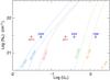 |
Fig. 5 Photoionization phase plot showing the ionization solutions for component 1 for all five epochs. The 2013 epoch solution is identical to the one shown in Fig. 3. For the 1998, 2002, and 2004 epochs we used the high SED (see Fig. 2) with the same abundances, and their ionization solutions are shown in blue crosses. Dashed lines represent Nion lower-limit that allow the phase-space above the line, while the dotted lines are upper-limits that allow the phase-space below the line (only the most restrictive constraints are shown). NH is fixed for all epochs at the value determined from the 2013 solution. For 1998, 2002 and 2004 the difference in UH values is determined by the ratio of fluxes at 1350 Å and the actual value is anchored by the observed Nion constraints. As explained in Sect. 3.3, the UH position of the 2011 epoch is less tightly constrained. The solution for each epoch satisfies all the Nion constraints for that epoch. |
In 1998 the AGN was in a high flux level of F = 6 (measured at 1350 Å rest-frame and given in units of 10-14 erg s-1 cm-2 Å-1). At that epoch the absorber only showed a Lyα trough necessitating log (UH)>~0.1 (otherwise a N v trough would be detected, see Fig. 5). In 2002 the AGN was in a medium flux level with F = 2, at which time the absorber showed C iv and N v troughs in addition to Lyα. In 2004 the AGN was at a historically low flux of F = 0.25. In that epoch a Si iii trough appeared in addition to the C iv, N v and Lyα troughs; however, a C ii trough did not appear. The combination of the Si iii and C ii constraints necessitates −1.3 < log (UH) < −1.15 (see Fig. 5). The change in log (UH) required by the photoionization models agrees remarkably well with the change in flux between the 1998 and 2004 epochs as log (F2004/F1998) = −1.4. Thus, a constant NH absorber yields an excellent fit for the absorption features from two epochs with the same SED (high SED in Fig. 5), but with very different UH values. Comparison of several key troughs between the five epochs is shown in Figs. A.2 and A.3. The 1350 Å flux measurements, plus observation details are given in Table A.1 and the derived column-densities for all the outflow features are given in Table A.2.
In 2013 the AGN flux was F = 3. With this flux level and assuming the same SED, the UH value should have been 50% higher than in 2002, and we would expect to see only C iv, N v and Lyα troughs. Instead we also detect Si iii, C ii, Si ii and Al ii. Therefore, the incident SED for component 1 must have changed, and indeed the 2013 soft X-ray flux is 25 times lower compared to that of the 2002 epoch (see Fig. 1 in Kaastra et al. 2014). This drop is caused by the newly observed obscurer close to the AGN, which does not fully cover the source (Kaastra et al. 2014). We found a good match to the UV absorption and soft X-ray flux with an SED that is similar to that of the high flux one longward of 1 Ry, but abruptly drops to 6% of that flux between 1 Ry and 1 keV (see Fig. 2). This picture is consistent with the transmitted flux resulting from the low-ionization, partial covering model of the obscurer derived in Kaastra et al. (2014). To complete the UV picture for component 1, in 2011 NGC 5548 showed F = 6, equal to that of the 1998 epoch. However, C iv and N v are clearly seen in the 2011 epoch but not any of the other ionic species seen in 2013. To explain this situation we assume that the obscurer was present at the 2011 epoch, but it only blocked somewhere between 50−90% of the emitted ionizing radiation between 1 Ry and 1 keV. The possible presence of a weaker X-ray obscurer is also suggested by broad absorption on the blue wing of the C IV emission line in 2011 that is weaker than that seen in 2013.
To summarize, a simple model based on a fixed total column-density absorber, reacting to changes in ionizing illumination, matches the very different phenomenology seen in all high-resolution UV spectra of component 1 spanning 16 years. Figure 6 gives a schematic illustration of the temporal model.
4. Components 2−6
We can derive distances (or limits of) for the other five outflow components and some constraints on the NH and UH of components 3 and 5. Figure 6 gives the velocities and distances of all six components, as well as a schematic illustration for their temporal behavior.
4.1. Constraining the distances
Components 2−6 do not show
absorption from excited levels (except for component 3, whose C ii/C ii*
troughs only yield a lower limit for ne). However, components 3 and 5 show
clear variations in their Si iii and Si iv troughs between our 2013 6 22
and 2013 8 1 observations, but not between the 2013 7 24 and 2013 8 1 ones, when we do see
changes in component 1. Using the formalism given in Sect. 4 of Arav et al. (2012), we can deduce the ne of these
components from the observed time lags. Suppose an absorber in photoionization equilibrium
experiences a sudden change in the incident ionizing flux such that Ii(t> 0) = (1 +
f)Ii(t
= 0), where −1 ≤
f ≤ ∞. Then the timescale for change in the ionic
fraction is given by: ![Mathematical equation: \begin{equation} t^* = \left[ -f \alpha_i n_{\rm e} \left( \frac{n_{i+1}}{n_i}- \frac{\alpha_{i-1}}{\alpha_i} \right) \right]^{-1}, \label{eq:trec} \end{equation}](/articles/aa/full_html/2015/05/aa25302-14/aa25302-14-eq83.png) (3)where αi is the recombination
rate of ion i
and ni is the fraction of a
given element in ionization stage i . From the 40 days that separate epochs showing
trough changes and the 7 days separating epochs with no change, we can deduce
3.5 < log (ne)
< 4.5 cm-3 for both components, otherwise their troughs would not
react to changes in incident ionizing flux in the observed way, despite the large changes
in incident ionizing flux over that period. Assuming a similar UH to that of
component 1 (see discussion below), this ne range yields distances of
5 <R<
15 pc. Similarly, component 6 shows C iv and N v
troughs in 2011 but not in 2002. This nine years timescale yields R< 100 pc. Component 2
and component 4 do not show changes in the UV absorption between any of the epochs.
Therefore, we can derive a lower limit for their distance of R> 130 pc.
(3)where αi is the recombination
rate of ion i
and ni is the fraction of a
given element in ionization stage i . From the 40 days that separate epochs showing
trough changes and the 7 days separating epochs with no change, we can deduce
3.5 < log (ne)
< 4.5 cm-3 for both components, otherwise their troughs would not
react to changes in incident ionizing flux in the observed way, despite the large changes
in incident ionizing flux over that period. Assuming a similar UH to that of
component 1 (see discussion below), this ne range yields distances of
5 <R<
15 pc. Similarly, component 6 shows C iv and N v
troughs in 2011 but not in 2002. This nine years timescale yields R< 100 pc. Component 2
and component 4 do not show changes in the UV absorption between any of the epochs.
Therefore, we can derive a lower limit for their distance of R> 130 pc.
4.2. Constraining NH and UH
It is not feasible to put physically interesting constraints on components 2, 4 and 6. First, they only show troughs from C iv, N v, and Lyα, which (based on our analysis of component 1) are probably highly saturated. Second, the ionization time-scales of components 2 and 4 are larger than 16 years. Therefore, even if a UH can be deduced from the measurements, it will only be a representative average value for a period of time larger than 16 years.
Figure 7 shows the NH–UH phase plot for component 3 based on the Nion reported in Table A.2 (the Lyα and C ivNion lower limits are trivially satisfied by the lower limit shown for the N vNion). The phase plot constraints given by the Nion measurements are mostly parallel to each other. Therefore, the NH–UH constraints are rather loose, allowing a narrow strip from log (NH) = 19.6 cm-2 and log (UH) = −2, to log (NH) = 21.5 cm-2 and log (UH) = −1.1. If we take the most probable value of log (UH) = −1.3, the distance estimate for component 3 will drop by 30% compared with the estimate of 5 <R< 15 pc, which used the log (UH) = −1.5 of component 1. For component 5, the situation is rather similar, as the detected Si iii and Si iv allow a narrow strip from log (NH) = 19.2 cm-2 and log (UH) = −1.8, to log (NH) = 20.7 cm-2 and log (UH) = −1.2, while the lowest χ2 is achieved at log (NH) = 20.7 cm-2 and log (UH) = −1.3.
5. Comparison with the warm absorber analysis
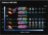 |
Fig. 6 An illustration of the physical, spatial and temporal conditions of the outflows seen in NGC 5548. Along the time axis we show the behavior of the emission source at the five UV epochs and give its UV flux values (measured at 1350 Å rest-frame and given in units of 10-14 erg s-1 cm-2 Å-1). The obscurer is situated at roughly 0.01 pc from the emission source and is only seen in 2011 and 2013 (it is much stronger in 2013). Outflow component 1 shows the most dramatic changes in its absorption troughs. Different observed ionic species are represented as colored zones within the absorbers. The trough changes are fully explained by our physical model shown in Fig. 5. Using component 1 C iii* troughs, which are only seen in the 2013 epoch, we determine its number density (see Fig. 4) to be log (ne) = 4.8 ± 0.1 cm-3, and therefore its distance, R = 3.5 pc. The distances for the other components are discussed in Sect. 4. Dimmer clouds represent epochs where components 2−6 did not show new absorption species compared with the 2002 epoch. |
Here we compare the physical characteristics inferred from the outflows’ UV diagnostics to the properties of the X-ray manifestation of the outflow known as the warm absorber (WA). Since the soft X-ray flux in our 2013 data is very low due to the appearance of the obscurer, we cannot characterize the WA that is connected with the six UV outflow components at that epoch. Our main inferences about the WA are from the 2002 epoch when we obtained simultaneous X-ray and UV spectra of the outflow (when no obscurer was present) that gave a much higher soft X-ray flux (compared with the 2013 observations) and allowed a detail modeling of the WA in that epoch (Steenbrugge et al. 2005; Kaastra et al. 2014). Due to the inherent complications of comparing analyses on different spectral regions (X-ray and UV) separated by 11 years (2002 and 2013), of a clearly time-dependent phenomenon, we defer a full comparison to a later paper (Ebrero et al., in prep.). Here we outline some of the main points in such a comparison, based on the analysis presented here and the published analysis of the WA (Steenbrugge et al. 2005; Kaastra et al. 2014) and discuss some of the similarities and challenges of such a combined analysis.
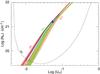 |
Fig. 7 Photoionization phase plot showing the ionization solution for component 3 epoch 2013. As for component 1, we use the obscured SED and assumed proto-solar metalicity (Lodders et al. 2009). Solid lines and associated colored bands represent the locus of UH,NH models, which predict the measured Nion, and their 1σ uncertainties, while the dashed line is the lower limit on the N v column-density that permits the phase-space above it. The blue cross is the best χ2 solution and is surrounded by a 1σχ2 blue contour. |
5.1. Kinematic similarity
There is kinematic correspondence between the UV absorption troughs in components 1–5 and the six ionization components (A−F) of the X-ray WA (Kaastra et al. 2014, see Table 1 here). X-ray components F and C span the width of UV component 1. X-ray component E matches UV component 2. The lowest ionization X-ray components, A and B comprise the full width of the blended UV troughs of components 3 and 4. Finally, X-ray component D kinematically matches UV component 5. However, as we show in point 2 below, this kinematic matching is physically problematic as the ionization parameters of WA components C, D, E and F are too high to produce observed troughs from C iv and N v that are observed in all the UV components.
Comparison between the UV and WA components.
5.2. Comparing similar ionization phases
We note that the X-ray analysis of the WA in the Chandra 2002 observations uses a different ionization parameter (ξ) than the UH we use here; where ξ ≡ L/ (nHr2) (erg cm s-1) with nH being the hydrogen number density, L the ionizing luminosity between 13.6 eV and 13.6 keV and r the distance from the central source. For the high SED, log (UH) = log (ξ) + 1.6. In Table 1, we give the log (UH) for the WA components. From the WA analysis and Fig. 5 here, we deduce that 90% of the WA material (components C, D, E and F in Table S2 of Kaastra et al. 2014) is in a too high ionization stage to produce measurable lines from the UV observed ions (e.g., C iv, N v). Only component A and B of the WA are at low enough ionization states to give rise to the UV observed material. The issue of pressure equilibrium between the different ionization phases is beyond the scope of this paper, and will be discussed in a forthcoming paper.
5.3. Assuming constant NH for the UV components and components A and B of the WA
Our temporal model for component 1 has a constant NH value in all the observed epochs, including 2002. The model also predicts the UH of the 2002 epoch (see Fig. 5). We can therefore compare the predictions of this model to the results of the reanalysis of the 2002 WA (Kaastra et al. 2014), provided that the NH for components A and B of the WA also did not change over the 11 years between the epochs. We note that since UV component 1 is the closest to the central source, the assumption of constant NH for the other UV components, over this 11 years time period, is reasonable (see discussion in Sect. 3.3). Therefore, we use the same ionization assumptions for UV components 3 and 5 as for component 1. That is, their NH is fixed to the 2013 value and their log (UH)2002 = log (UH)2013 + 1.1, which are the values we list in Table 1. We do not have empirical constraints on the distances of WA components A-F from the central source.
5.4. Comparing UV components 1 and 3 to components A and B of the WA.
Using proto-Solar abundances (Lodders et al.
2009), our 2002 model prediction for UV component 1 has
cm-2, and an ionization parameter
of  (see Sect. 3.1 and Fig. 5). This model gives a good
match for the UV data of that epoch (2002) and its log (UH) is in
between those of WA components A [log (UH) = −0.8] and B [log (UH) =
−0.1]. However, there are two inconsistencies between the models. First,
components A and B have a total log (NH) = 20.95 ± 0.1 cm-2 or about 2σ disagreement with that of
UV component 1. This discrepancy is mainly due to the limit on the
O viiNion that arises from the bound-free
edge of this ion in the X-ray data. In the WA model, about 95% of the
O viiNion arises from components A and B.
Second, the reported velocity centroids for WA components A and B (−588 ± 34 km s-1 and −547 ± 31 km s-1, respectively) are in
disagreement with the velocity centroids of UV component 1 (−1160 km s-1) and its 300
km s-1 width.
(see Sect. 3.1 and Fig. 5). This model gives a good
match for the UV data of that epoch (2002) and its log (UH) is in
between those of WA components A [log (UH) = −0.8] and B [log (UH) =
−0.1]. However, there are two inconsistencies between the models. First,
components A and B have a total log (NH) = 20.95 ± 0.1 cm-2 or about 2σ disagreement with that of
UV component 1. This discrepancy is mainly due to the limit on the
O viiNion that arises from the bound-free
edge of this ion in the X-ray data. In the WA model, about 95% of the
O viiNion arises from components A and B.
Second, the reported velocity centroids for WA components A and B (−588 ± 34 km s-1 and −547 ± 31 km s-1, respectively) are in
disagreement with the velocity centroids of UV component 1 (−1160 km s-1) and its 300
km s-1 width.
UV component 3 has a velocity centroid at −640 km s-1 and a width of ~200 km s-1, and therefore is a better velocity match with WA components A and B. The large uncertainties in the inferred NH and UH for UV component 3 (see Fig. 7 and Table 1), make these values consistent with the NH and UH deduced for WA components A and B. However, the uncertainties also allow UV component 3 to have a negligible NH compared to WA components A and B.
We note that with the current analyses, the better the agreement between UV component 3 and WA components A and B, the worse is the disagreement between UV component 1 and WA components A and B. This is because UV component 1 already predicts higher values of NH and O viiNion than are measured in WA components A and B, and the kinematics of the deduced O viiNion disagree considerably. In points 5 and 6 below we identify two possible ways to alleviate and even eliminate these apparent discrepancies.
5.5. Existence of considerable O VII Nion at the velocity of UV component 1
The 2002 X-ray spectra presented by Steenbrugge et al. (2005) consist of two different data sets that were acquired in the same week: 170 ks observations taken with the High Energy Transmission Grating Spectrometer (HETGS) and 340 ks observations with the Low Energy Transmission Grating Spectrometer (LETGS). Figure 2 in Steenbrugge et al. (2005) shows some of the low ionization WA troughs in velocity presentation, where the dotted lines show the position of the UV components (with somewhat different velocity values than we use here due to the use of a slightly different systemic redshift for the object). The LETGS data of the O vii and O v troughs are consistent with one main kinematic component matching the velocity of UV component 3. However, the more noisy but higher resolution HETGS data for the same transitions, show two subtroughs: one corresponding to UV component 1 and one to UV component 3. Therefore, it is possible that much of the O viiNion is associated with UV component 1.
5.6. Abundances considerations
As mentioned in Sect. 3, for the UV analysis, we use pure proto-Solar abundances (Lodders et al. 2009), which well-match the measured Nion from the UV data. But these models produce considerably more O viiNion in the 2002 epoch, than the measured O viiNion in the warm absorber data. However, the NH (and therefore also the O viiNion) of UV component 1 is critically dependent on the assumed phosphorus abundance. Ionization models with all elements having proto-Solar abundances except phosphorus, for which we assume twice proto-Solar abundance, preserve the fit to the UV data (at 1/3 the NH value) and at the same time match the O viiNion measured in the X-ray warm absorber at the 2002 epoch. Larger over-abundances of phosphorus further reduce the NH value and therefore the predicted O viiNion for the 2002 epoch.
But are such assumed abundances physically reasonable? AGN outflows are known to have abundances higher by factors of two (Arav et al. 2007) and even ten (Gabel et al. 2006) compared with the proto-Solar values. In particular, phosphorus abundance in AGN outflows, relative to other metals, can be a factor of several higher than in proto-Solar abundances (see Sect. 4.1 in Arav et al. 2001). Furthermore, the theoretical expectations for the value of chemical abundances in an AGN environment as a function of metalicity are highly varied. The leading models can differ about relative abundances values by factors of three or more (e.g., comparing the values of Hamann & Ferland 1993; Ballero et al. 2008).
We conclude that if roughly half of the observed O viiNion is associated with UV component 1 (as discussed in point 5), and if the relative abundance of phosphorus to oxygen is twice solar or larger, than the NH, UH and velocity distribution of the WA and UV outflowing gas can be consistent.
6. Discussion
6.1. Comparison with Crenshaw et al. (2009)
Here we compare our results with previous work by Crenshaw et al. (2009, hereafter C09) on the enduring outflow in NGC 5548. For the first time a simple model of a constant NH absorber yields a physical picture that is consistent with the substantial trough variations seen in all epochs of high-resolution UV spectral observations. The trough changes are explained solely by the observed differences in the incident ionizing flux. In addition, we determine robust distances for (or limits on) all six kinematic components.
Our results differ considerably from those previously found for this outflow in C09. The HST epochs of 1998, 2002 and 2004 were analyzed by C09. In Table 2 we show for component 1 the deduced log (NH) and log (UH) values for these 3 epochs, for both C09 (see their Table 6) and this work (see Fig. 5 here). It is clear that we derive very different parameters than those of C09.
The main reason for these differences is the reliability of the measured ionic column censities (Nion), which are used as input in photoionization models. Both works use CLOUDY, assume the same abundances and use a similar SED. C09 base their photoionization solution on the Nion of C iv and N v (see C09 Table 5). We obtain similar C iv and N vNion values in these epochs (see Table A.2 here), but we only use them as lower limits. The new diagnostic troughs seen during the 2013 campaign (especially P v) demonstrate this crucial point. The existence of similar depth C iv and P v troughs in component 1 is evidence that the actual C ivNion is at least a factor of 100 larger than the lower limit (see discussion in Borguet et al. 2012a). A similar situation occurs for N v. This assertion is confirmed quantitatively by our full photoionization models. With such large saturation factors, photoionization solutions for this outflow based on the trough-derived C iv and N vNion are unreliable.
Comparing the photoionization solutions for component 1.
Examining the results for the 2004 epoch demonstrates these issues. Using the C iv and N vNion values of C09 for component 1, we can reproduce their log (UH) and log (NH) parameters. However, the 2004 HST spectrum shows clear Si iii troughs in components 1 and 3 (see Fig. A.3f here) that are unaccounted for in C09. The C09 solution shown in Table 2 is incompatible with the Si iiiNion measurement, even if that trough is unsaturated. To reproduce the Si iii measurement using the C09 log (NH) = 20.35 cm-2, log (UH) need to be −1.7 ± 0.1 instead of the C09 value of log (UH) = −0.55. However, at log (NH) = 20.35 cm-2 and log (UH) = −1.7, CLOUDY yields a C ivNion that is 100 times larger than the value C09 deduce from the observations (see their Table 5).
In conclusion, our improved physical modeling is due to powerful diagnostics that were revealed during the 2013 campaign, establishing that many of the observed troughs are highly saturated; and also because C09 did not account for the Si iii troughs associated with components 1 and 3 in the 2004 data.
6.2. Implications for BALQSO variability studies
Our multiwavelength campaign has significant consequences for studies of absorption trough variability in quasar outflows, and in particular for the intensive studies of trough variability in broad absorption line (BAL) quasars (e.g., Barlow et al. 1992; Capellupo et al. 2012; Filiz Ak et al. 2013, and references therein). AGN outflow absorption systems with different velocity width, and different AGN luminosities, share similar physical characteristics (e.g., ionization states, trough variability time scales, trough variability pattern, solar or larger metallicity, non-black saturation in the troughs). Therefore, we can can make a comparison between the mechanisms in the narrow outflow of NGC 5548 to that of BALs in QSOs.
As discussed in Sect. 3.3, the two main proposed mechanisms for trough variability are (1) reaction to changes in ionizing flux of a constant absorber (which is the model we successfully use to explain the NGC 5548 outflow trough changes); and (2) absorber motion across the line of sight (e.g., Gabel et al. 2003), which as we demonstrated, cannot explain the variability of the enduring, narrow-trough outflow in NGC 5548 (see Sect. 3.3).
In some BALQSO cases the rest-frame UV flux around 1350 Å does not change appreciably between the studied epochs while significant trough variability is observed. This behavior is taken as an argument against mechanism (1) (e.g., Barlow et al. 1992; Filiz Ak et al. 2013) as the ionizing flux (below 912 Å) is assumed to correlate with the longer wavelength UV flux. However, our simultaneous UV/X-ray observations show a clear case where the ionizing photon flux drops by a factor of 25 between the 2002 and 2013 epochs, while the 1350 Å UV flux actually increases by 50%.
Mechanism (1) is a simpler explanation for cases where velocity-separated outflow troughs change in the same way between different epochs (i.e., when all troughs become either shallower or deeper; Capellupo et al. 2012; Filiz Ak et al. 2013). As we demonstrated, the objection to this model based on the assumed correlation between the rest-frame UV flux around 1350 Å and the ionizing flux might not be valid. Therefore, due to its simplicity, mechanism (1) is a strong contender for interpreting trough variability data of quasar outflows.
We note that the above discussion does not exclude the possibility of trough variability due to absorber motion across the line of sight, in some cases. Indeed it is possible that this mechanism explains the variability in the newly discovered broad UV absorption in NGC 5548, as argued in Kaastra et al. (2014).
The data set of NGC 5548 (spanning five high-resolution spectroscopic epochs between 1998 and 2013) gives high S/N spectra of UV absorption troughs that arise from many different ions, and simultaneously yields the crucial soft X-ray flux that is responsible for the ionization of the outflow. Such data can constrain trough variability models far better than the standard variability data sets where one or two rest-frame UV BAL are observed at two (and less frequently in more) epochs (e.g., Capellupo et al. 2012; Filiz Ak et al. 2013).
6.3. Implications for the X-ray obscurer
Our results about the enduring outflow have implications for the X-ray obscurer and the broad UV absorption discovered by Kaastra et al. (2014). The derived transmission for the X-ray obscurer is consistent with the SED required for the 2013 spectrum, thus showing that the obscurer is closer to the super massive black holes than 3.5 pc, and that its shadow influences the conditions in the more distant narrow UV absorbers.
7. Summary
In 2013 we executed the most comprehensive multiwavelength spectroscopic campaign on any AGN to date, directed at NGC 5548. This paper presents the analysis’ results from our HST/COS data of the enduring UV outflow, which is detected in six distinct kinematic components. Our campaign revealed an unusually strong X-ray obscuration. The resulting dramatic decrease in incident ionizing flux on the outflow allowed us to construct a comprehensive physical, spatial and temporal picture for the well-studied AGN wind in this object. Our main findings are listed below (see Fig. 6 for a graphic illustration of our results).
-
1.
Our best constraints are obtained forcomponent 1 (the highest velocity component). Itis situated at
pc from the central source, has a
total hydrogen column-density of cm-2, an ionization parameter
of , and an electron number density of
log (ne) =
4.8 ± 0.1 cm-3. This component probably carries the largest
NH associated with the UV outflow. See
Sects. 3.1 and 3.2. -
2.
For component 1 a simple model based on a fixed total column-density absorber, reacting to changes in ionizing illumination, matches the very different ionization states seen at five spectroscopic epochs spanning 16 years. See Sect. 3.3.
-
3.
The distance and number density of component 1 are similar to those of the narrow-emitting-line-region in this object (Peterson et al. 2013). See Sect. 3.2.
-
4.
The wealth of observational constraints makes our changes-of-ionization model a leading contender for interpreting trough variability data of quasar outflows, in particular BAL variability. See Sect. 6.2.
-
5.
Components 3 and 5 are situated between 5−15 pc from the central source, component 6 is closer than 100 pc and components 2 and 4 are further out than 130 pc. See Sect. 4.
Online material
Appendix A: Ionic column-density measurements
The column-density associated with a given ion as a function of the radial velocity
v is
defined as: 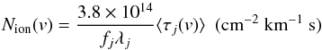 (A.1)where fj, λj and ⟨
τj(v)
⟩ are respectively the oscillator strength, the rest wavelength and
the average optical depth across the emission source of the line j for which the optical
depth solution is derived (see Edmonds et al.
2011). The optical depth solution across a trough is found for a given ion by
assuming an absorber model. As shown in Edmonds et al.
(2011), the major uncertainty on the derived column-densities comes from the
choice of absorption model. In this study we investigate the outflow properties using
column-densities derived from three common absorber models.
(A.1)where fj, λj and ⟨
τj(v)
⟩ are respectively the oscillator strength, the rest wavelength and
the average optical depth across the emission source of the line j for which the optical
depth solution is derived (see Edmonds et al.
2011). The optical depth solution across a trough is found for a given ion by
assuming an absorber model. As shown in Edmonds et al.
(2011), the major uncertainty on the derived column-densities comes from the
choice of absorption model. In this study we investigate the outflow properties using
column-densities derived from three common absorber models.
Assuming a single, homogeneous emission source of intensity F0, the simplest absorber model is the one where a homogeneous absorber parameterized by a single optical depth fully covers the photon source. In that case, known as the apparent optical depth scenario (AOD), the optical depth of a line j as a function of the radial velocity v in the trough is simply derived by the inversion of the Beer-Lambert law: τj(v) = −ln(Fj(v) /F0(v)), where Fj(v) is the observed intensity of the line.
Early studies of AGN outflows pointed out the inadequacy of such an absorber model, specifically its inability to account for the observed departure of measured optical depth ratio between the components of typical doublet lines from the expected laboratory line strength ratio R = λifi/λjfj. Two parameter absorber models have been developed to explain such discrepancies.
Observations and flux values for all epochs.
The partial covering model (e.g. Hamann et al.
1997; Arav et al. 1999, 2002, 2005)
assumes that only a fraction C of the emission source is covered by absorbing
material with constant optical depth τ. In that case, the intensity observed for a
line j of a
chosen ion can be expressed as  (A.2)Our third choice are inhomogeneous absorber
models. In that scenario, the emission source is totally covered by a smooth
distribution of absorbing material across its spatial dimension x. Assuming the typical
power law distribution of the optical depth τ(x) =
τmaxxa
(de Kool et al. 2002; Arav et al. 2005, 2008), the
observed intensity observed for a line j of a chosen ion is given by
(A.2)Our third choice are inhomogeneous absorber
models. In that scenario, the emission source is totally covered by a smooth
distribution of absorbing material across its spatial dimension x. Assuming the typical
power law distribution of the optical depth τ(x) =
τmaxxa
(de Kool et al. 2002; Arav et al. 2005, 2008), the
observed intensity observed for a line j of a chosen ion is given by  (A.3)Once the line profiles have been binned on
a common velocity scale (we choose a resolution dv = 20 km s-1,
slightly lower than the resolution of COS), a velocity dependent solution can be
obtained for the couple of parameters (C,τj)
or (a,τmax) of both
absorber models as long as one observes at least two lines from a given ion, sharing the
same lower energy level. Once the velocity dependent solution is computed, the
corresponding column density is derived using Eq. (A.1) where ⟨
τj(v) ⟩ =
Cion(v)τj(v)
for the partial covering model and ⟨
τj(v) ⟩ =
τmax,j(v) /
(aion(v) + 1) for the
power law distribution. Note that the AOD solution can be computed for any line (singlet
or multiplet), without further assumption on the model, but will essentially give a
lower limit on the column-density when the expected line strength ratio observed is
different from the laboratory value.
(A.3)Once the line profiles have been binned on
a common velocity scale (we choose a resolution dv = 20 km s-1,
slightly lower than the resolution of COS), a velocity dependent solution can be
obtained for the couple of parameters (C,τj)
or (a,τmax) of both
absorber models as long as one observes at least two lines from a given ion, sharing the
same lower energy level. Once the velocity dependent solution is computed, the
corresponding column density is derived using Eq. (A.1) where ⟨
τj(v) ⟩ =
Cion(v)τj(v)
for the partial covering model and ⟨
τj(v) ⟩ =
τmax,j(v) /
(aion(v) + 1) for the
power law distribution. Note that the AOD solution can be computed for any line (singlet
or multiplet), without further assumption on the model, but will essentially give a
lower limit on the column-density when the expected line strength ratio observed is
different from the laboratory value.
UV column-densities for the outflow components in NGC 5548.
 |
Fig. A.1 2013 spectrum of NGC 5548. The vertical axis is the flux in units of 10-14 erg s-1 cm-2 Å-1, and the quasar-rest-frame and observer-frame wavelengths are given in Angstroms on the top and bottom of each sub-plot, respectively. Each of the six kinematic components of the outflow shows absorption troughs from several ions. We place a vertical mark at the expected center of each absorption trough (following the velocity template of Si iv and N v) and state the ion, rest-wavelength and component number (C1–C6). We also assign a color to each component number that ranges from blue (C1) to red (C6). Absorption lines from the ISM are likewise marked in black with dashed lines. |
 |
Fig. A.1 continued. |
 |
Fig. A.1 continued. |
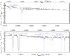 |
Fig. A.1 continued. |
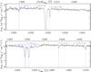 |
Fig. A.1 continued. |
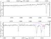 |
Fig. A.1 continued. |
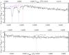 |
Fig. A.1 continued. |
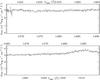 |
Fig. A.1 continued. |
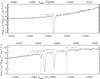 |
Fig. A.1 continued. |
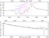 |
Fig. A.1 continued. |
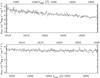 |
Fig. A.1 continued. |
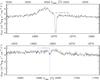 |
Fig. A.1 continued. |
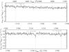 |
Fig. A.1 continued. |
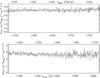 |
Fig. A.1 continued. |
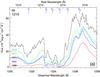 |
Fig. A.2 Spectrum of NGC 5548 during the five epochs of observation. The 2013 spectrum is obtained by co-adding visits 1 through 5. Spectral regions where absorption troughs from five ions are shown in sub-plots a) through e) and the six kinematic components associated with such absorption are labelled C1 through C6. |
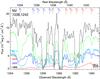 |
Fig. A.2 continued. |
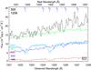 |
Fig. A.2 continued. |
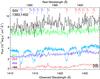 |
Fig. A.2 continued. |
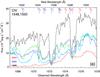 |
Fig. A.2 continued. |
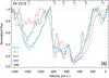 |
Fig. A.3 Normalized spectrum of NGC 5548 during the five epochs of observation, plotted in the velocity rest-frame of the quasar (same annotation as Fig. A.2). |
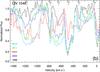 |
Fig. A.3 continued. |
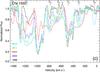 |
Fig. A.3 continued. |
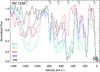 |
Fig. A.3 continued. |
 |
Fig. A.3 continued. |
 |
Fig. A.3 continued. |
 |
Fig. A.3 continued. |
 |
Fig. A.3 continued. |
Acknowledgments
This work was supported by NASA through grants for HST program number 13184 from the Space Telescope Science Institute, which is operated by the Association of Universities for Research in Astronomy, Incorporated, under NASA contract NAS5-26555. SRON is supported financially by NWO, the Netherlands Organization for Scientific Research. M.M. acknowledges the support of a Studentship Enhancement Programme awarded by the UK Science & Technology Facilities Council (STFC). P.-O.P. and F.U. thank financial support from the CNES and from the CNRS/PICS. F.U. acknowledges Ph.D. funding from the VINCI program of the French-Italian University. K.C.S. wants to acknowledge financial support from the Fondo Fortalecimiento de la Productividad Cientfica VRIDT 2013. E.B. is supported by grants from Israel’s MoST, ISF (1163/10), and I-CORE program (1937/12). J.M. acknowledges funding from CNRS/PNHE and CNRS/PICS in France. G.M. and F.U. acknowledge financial support from the Italian Space Agency under grant ASI/INAF I/037/12/0-011/13. B.M.P. acknowledges support from the US NSF through grant AST-1008882. M.C., S.B., G.M. and A.D.R. acknowledge INAF/PICS support. G.P. acknowledges support via an EU Marie Curie Intra-European fellowship under contract no. FP-PEOPLE-2012-IEF-331095. M.W. acknowledges the support of a Ph.D. studentship awarded by the UK Science & Technology Facilities Council (STFC). The data used in this research are stored in the public archives of the satellites that are involved. We thank the International Space Science Institute (ISSI) in Bern for support. This work is based on observations obtained with XMM-Newton, an ESA science mission with instruments and contributions directly funded by ESA Member States and the USA (NASA). It is also based on observations with INTEGRAL, an ESA project with instrument and science data center funded by ESA member states (especially the PI countries: Denmark, France, Germany, Italy, Switzerland, Spain), Czech Republic, and Poland and with the participation of Russia and the USA. This work made use of data supplied by the UK Swift Science Data Centre at the University if Leicester. This research made use of the Chandra Transmission Grating Catalog and archive (http://tgcat.mit.edu). This research has made use of data obtained with the NuSTAR mission, a project led by the California Institute of Technology (Caltech), managed by the Jet Propulsion Laboratory (JPL) and funded by NASA, and has utilized the NuSTAR Data Analysis Software (NUSTARDAS) jointly developed by the ASI Science Data Center (ASDC, Italy) and Caltech (USA). Figure 6 was created by Ann Feild from STScI.
References
- Arav, N., Becker, R. H., Laurent-Muehleisen, S. A., et al. 1999, ApJ, 524, 566 [NASA ADS] [CrossRef] [Google Scholar]
- Arav, N., de Kool, M., Korista, K. T., et al. 2001, ApJ, 561, 118 [NASA ADS] [CrossRef] [Google Scholar]
- Arav, N., Korista, K. T., & de Kool, M. 2002, ApJ, 566, 699 [NASA ADS] [CrossRef] [Google Scholar]
- Arav, N., Kaastra, J., Kriss, G. A., et al. 2005, ApJ, 620, 665 [NASA ADS] [CrossRef] [Google Scholar]
- Arav, N., Gabel, J. R., Korista, K. T., et al. 2007, ApJ, 658, 829 [NASA ADS] [CrossRef] [Google Scholar]
- Arav, N., Moe, M., Costantini, E., et al. 2008, ApJ, 681, 954 [NASA ADS] [CrossRef] [Google Scholar]
- Arav, N., Edmonds, D., Borguet, B., et al. 2012, A&A, 544, A33 [NASA ADS] [CrossRef] [EDP Sciences] [Google Scholar]
- Arav, N., Borguet, B., Chamberlain, C., Edmonds, D., & Danforth, C. 2013, MNRAS, 436, 3286 [NASA ADS] [CrossRef] [Google Scholar]
- Ballero, S. K., Matteucci, F., Ciotti, L., Calura, F., & Padovani, P. 2008, A&A, 478, 335 [NASA ADS] [CrossRef] [EDP Sciences] [Google Scholar]
- Barlow, T. A., Junkkarinen, V. T., Burbidge, E. M., et al. 1992, ApJ, 397, 81 [NASA ADS] [CrossRef] [Google Scholar]
- Borguet, B. C. J., Edmonds, D., Arav, N., Benn, C., & Chamberlain, C. 2012a, ApJ, 758, 69 [NASA ADS] [CrossRef] [Google Scholar]
- Borguet, B. C. J., Edmonds, D., Arav, N., Dunn, J., & Kriss, G. A. 2012b, ApJ, 751, 107 [NASA ADS] [CrossRef] [Google Scholar]
- Borguet, B. C. J., Arav, N., Edmonds, D., Chamberlain, C., & Benn, C. 2013, ApJ, 762, 49 [NASA ADS] [CrossRef] [Google Scholar]
- Capellupo, D. M., Hamann, F., Shields, J. C., Rodríguez Hidalgo, P., & Barlow, T. A. 2012, MNRAS, 422, 3249 [NASA ADS] [CrossRef] [Google Scholar]
- Ciotti, L., Ostriker, J. P., & Proga, D. 2010, ApJ, 717, 708 [NASA ADS] [CrossRef] [Google Scholar]
- Costantini, E., Kaastra, J. S., Arav, N., et al. 2007, A&A, 461, 121 [NASA ADS] [CrossRef] [EDP Sciences] [Google Scholar]
- Crenshaw, D. M., Kraemer, S. B., Boggess, A., et al. 1999, ApJ, 516, 750 [NASA ADS] [CrossRef] [Google Scholar]
- Crenshaw, D. M., Kraemer, S. B., Gabel, J. R., et al. 2003, ApJ, 594, 116 [NASA ADS] [CrossRef] [Google Scholar]
- Crenshaw, D. M., Kraemer, S. B., Schmitt, H. R., et al. 2009, ApJ, 698, 281 [NASA ADS] [CrossRef] [Google Scholar]
- de Kool, M., Korista, K. T., & Arav, N. 2002, ApJ, 580, 54 [NASA ADS] [CrossRef] [Google Scholar]
- de Vaucouleurs, G., de Vaucouleurs, A., Corwin, Jr., H. G., et al. 1991, Third Reference Catalogue of Bright Galaxies, Vol. I: Explanations and references, Vol. II: Data for galaxies between 0h and 12h. Vol. III: Data for galaxies between 12h and 24h (Springer) [Google Scholar]
- Dere, K. P., Landi, E., Mason, H. E., Monsignori Fossi, B. C., & Young, P. R. 1997, A&AS, 125, 149 [NASA ADS] [CrossRef] [EDP Sciences] [Google Scholar]
- Edmonds, D., Borguet, B., Arav, N., et al. 2011, ApJ, 739, 7 [NASA ADS] [CrossRef] [Google Scholar]
- Faucher-Giguère, C.-A., Quataert, E., & Murray, N. 2012, MNRAS, 420, 1347 [NASA ADS] [CrossRef] [Google Scholar]
- Ferland, G. J., Porter, R. L., van Hoof, P. A. M., et al. 2013, Rev. Mex. Astron. Astrofis., 49, 137 [Google Scholar]
- Filiz Ak, N., Brandt, W. N., Hall, P. B., et al. 2013, ApJ, 777, 168 [NASA ADS] [CrossRef] [Google Scholar]
- Gabel, J. R., Crenshaw, D. M., Kraemer, S. B., et al. 2003, ApJ, 583, 178 [NASA ADS] [CrossRef] [Google Scholar]
- Gabel, J. R., Kraemer, S. B., Crenshaw, D. M., et al. 2005, ApJ, 631, 741 [NASA ADS] [CrossRef] [Google Scholar]
- Gabel, J. R., Arav, N., & Kim, T. 2006, ApJ, 646, 742 [NASA ADS] [CrossRef] [Google Scholar]
- Green, J. C., Froning, C. S., Osterman, S., et al. 2012, ApJ, 744, 60 [NASA ADS] [CrossRef] [Google Scholar]
- Hamann, F., & Ferland, G. 1993, ApJ, 418, 11 [NASA ADS] [CrossRef] [Google Scholar]
- Hamann, F., Barlow, T. A., Junkkarinen, V., & Burbidge, E. M. 1997, ApJ, 478, 80 [NASA ADS] [CrossRef] [Google Scholar]
- Hopkins, P. F., & Elvis, M. 2010, MNRAS, 401, 7 [NASA ADS] [CrossRef] [Google Scholar]
- Kaastra, J. S., Detmers, R. G., Mehdipour, M., et al. 2012, A&A, 539, A117 [NASA ADS] [CrossRef] [EDP Sciences] [Google Scholar]
- Kaastra, J. S., Kriss, G. A., Cappi, M., et al. 2014, Science, 345, 64 [NASA ADS] [CrossRef] [Google Scholar]
- Korista, K. T., Alloin, D., Barr, P., et al. 1995, ApJS, 97, 285 [NASA ADS] [CrossRef] [Google Scholar]
- Landi, E., Young, P. R., Dere, K. P., Del Zanna, G., & Mason, H. E. 2013, ApJ, 763, 86 [NASA ADS] [CrossRef] [Google Scholar]
- Lodders, K., Palme, H., & Gail, H.-P. 2009, in Landolt-Börnstein − Group VI Astronomy and Astrophysics Numerical Data and Functional Relationships in Science and Technology Volume, ed. J. E. Trümper, 44 [Google Scholar]
- Mehdipour, M. M., Kaastra, J., Kriss, J., et al. 2014, in The X-ray Universe 2014, ed. J.-U. Ness, Online at http://xmm.esac.esa.int/external/xmm_science/workshops/2014symposium/, 34 [Google Scholar]
- Ostriker, J. P., Choi, E., Ciotti, L., Novak, G. S., & Proga, D. 2010, ApJ, 722, 642 [NASA ADS] [CrossRef] [Google Scholar]
- Pancoast, A., Brewer, B. J., Treu, T., et al. 2014, MNRAS, 445, 3073 [NASA ADS] [CrossRef] [Google Scholar]
- Peterson, B. M., Denney, K. D., De Rosa, G., et al. 2013, ApJ, 779, 109 [NASA ADS] [CrossRef] [Google Scholar]
- Schlafly, E. F., & Finkbeiner, D. P. 2011, ApJ, 737, 103 [NASA ADS] [CrossRef] [Google Scholar]
- Soker, N., & Meiron, Y. 2011, MNRAS, 411, 1803 [NASA ADS] [CrossRef] [Google Scholar]
- Steenbrugge, K. C., Kaastra, J. S., Crenshaw, D. M., et al. 2005, A&A, 434, 569 [NASA ADS] [CrossRef] [EDP Sciences] [Google Scholar]
All Tables
All Figures
|
Fig. 1 Intrinsic absorption features in the 2013 COS spectrum of NGC 5548. Normalized relative fluxes are plotted as a function of velocity relative to the systemic redshift of z = 0.017175, top to bottom: Si iiiλ1206, Si ivλλ1394,1403, C ivλλ1548,1550, N vλλ1238,1242, and Ly α, as a function of rest-frame velocity. For the doublets the red and blue components are shown in red and blue, respectively. Dotted vertical lines indicate the velocities of the absorption components numbered as in Crenshaw et al. (2003). |
| In the text | |
|
Fig. 2 Adopted NGC 5548 SEDs. In black we show the SED for NGC 5548 in 2002 at an unobscured X-ray flux (hereafter “high SED”, from Steenbrugge et al. 2005). In blue we show the SED appropriate to the 2013 epoch, where for the same flux at 1000 Å, the new X-ray obscurer reduced the ionizing flux by a factor of 17 between 1 Ry and 1 keV (obscured SED). The ionization potentials for destruction of some of the prominent observed species are shown by the vertical lines. |
| In the text | |
|
Fig. 3 Photoionization phase plot showing the ionization solution for component 1 epoch 2013. We use the obscured SED and assumed proto-solar metalicity (Lodders et al. 2009). Solid lines and associated colored bands represent the locus of UH,NH models, which predict the measured Nion, and their 1σ uncertainties. The black dot is the best solution and is surrounded by a 1σχ2 contour. |
| In the text | |
|
Fig. 4 a) Absorption spectrum for the C iii* 1175 Å multiplet. The 2013 COS spectrum shows clear and relatively unblended individual troughs from the J = 2 and J = 0 levels, but no contribution from the J = 1 level that is populated at higher densities (see panel c)). b) Absorption spectrum for the Si iii* 1298 Å multiplet (similar in level structure to the C iii* 1175 Å multiplet). The 2013 COS spectrum shows shallow but highly significant individual troughs from the J = 2 and J = 0 levels, but again no contribution from the J = 1 level that is populated at higher densities. c) C iii* and Si iii* level population ratios, theory and measurements. The computed populations for the J = 2/J = 0 and J = 1/J = 0 are plotted as a function of electron number density for both ions (see text for elaboration). The crosses show the measured ratios for the J = 2/J = 0 ratio of both ions. From the C iii* ratios we infer log (ne) = 4.8 ± 0.1 cm-3, where the error includes both statistical and systematic effects. This value is fully consistent with the one inferred from the Si iii* ratio, where in the case of Si iii* the statistical error is larger since the troughs are much shallower. |
| In the text | |
|
Fig. 5 Photoionization phase plot showing the ionization solutions for component 1 for all five epochs. The 2013 epoch solution is identical to the one shown in Fig. 3. For the 1998, 2002, and 2004 epochs we used the high SED (see Fig. 2) with the same abundances, and their ionization solutions are shown in blue crosses. Dashed lines represent Nion lower-limit that allow the phase-space above the line, while the dotted lines are upper-limits that allow the phase-space below the line (only the most restrictive constraints are shown). NH is fixed for all epochs at the value determined from the 2013 solution. For 1998, 2002 and 2004 the difference in UH values is determined by the ratio of fluxes at 1350 Å and the actual value is anchored by the observed Nion constraints. As explained in Sect. 3.3, the UH position of the 2011 epoch is less tightly constrained. The solution for each epoch satisfies all the Nion constraints for that epoch. |
| In the text | |
|
Fig. 6 An illustration of the physical, spatial and temporal conditions of the outflows seen in NGC 5548. Along the time axis we show the behavior of the emission source at the five UV epochs and give its UV flux values (measured at 1350 Å rest-frame and given in units of 10-14 erg s-1 cm-2 Å-1). The obscurer is situated at roughly 0.01 pc from the emission source and is only seen in 2011 and 2013 (it is much stronger in 2013). Outflow component 1 shows the most dramatic changes in its absorption troughs. Different observed ionic species are represented as colored zones within the absorbers. The trough changes are fully explained by our physical model shown in Fig. 5. Using component 1 C iii* troughs, which are only seen in the 2013 epoch, we determine its number density (see Fig. 4) to be log (ne) = 4.8 ± 0.1 cm-3, and therefore its distance, R = 3.5 pc. The distances for the other components are discussed in Sect. 4. Dimmer clouds represent epochs where components 2−6 did not show new absorption species compared with the 2002 epoch. |
| In the text | |
|
Fig. 7 Photoionization phase plot showing the ionization solution for component 3 epoch 2013. As for component 1, we use the obscured SED and assumed proto-solar metalicity (Lodders et al. 2009). Solid lines and associated colored bands represent the locus of UH,NH models, which predict the measured Nion, and their 1σ uncertainties, while the dashed line is the lower limit on the N v column-density that permits the phase-space above it. The blue cross is the best χ2 solution and is surrounded by a 1σχ2 blue contour. |
| In the text | |
|
Fig. A.1 2013 spectrum of NGC 5548. The vertical axis is the flux in units of 10-14 erg s-1 cm-2 Å-1, and the quasar-rest-frame and observer-frame wavelengths are given in Angstroms on the top and bottom of each sub-plot, respectively. Each of the six kinematic components of the outflow shows absorption troughs from several ions. We place a vertical mark at the expected center of each absorption trough (following the velocity template of Si iv and N v) and state the ion, rest-wavelength and component number (C1–C6). We also assign a color to each component number that ranges from blue (C1) to red (C6). Absorption lines from the ISM are likewise marked in black with dashed lines. |
| In the text | |
|
Fig. A.1 continued. |
| In the text | |
|
Fig. A.1 continued. |
| In the text | |
|
Fig. A.1 continued. |
| In the text | |
|
Fig. A.1 continued. |
| In the text | |
|
Fig. A.1 continued. |
| In the text | |
|
Fig. A.1 continued. |
| In the text | |
|
Fig. A.1 continued. |
| In the text | |
|
Fig. A.1 continued. |
| In the text | |
|
Fig. A.1 continued. |
| In the text | |
|
Fig. A.1 continued. |
| In the text | |
|
Fig. A.1 continued. |
| In the text | |
|
Fig. A.1 continued. |
| In the text | |
|
Fig. A.1 continued. |
| In the text | |
|
Fig. A.2 Spectrum of NGC 5548 during the five epochs of observation. The 2013 spectrum is obtained by co-adding visits 1 through 5. Spectral regions where absorption troughs from five ions are shown in sub-plots a) through e) and the six kinematic components associated with such absorption are labelled C1 through C6. |
| In the text | |
|
Fig. A.2 continued. |
| In the text | |
|
Fig. A.2 continued. |
| In the text | |
|
Fig. A.2 continued. |
| In the text | |
|
Fig. A.2 continued. |
| In the text | |
|
Fig. A.3 Normalized spectrum of NGC 5548 during the five epochs of observation, plotted in the velocity rest-frame of the quasar (same annotation as Fig. A.2). |
| In the text | |
|
Fig. A.3 continued. |
| In the text | |
|
Fig. A.3 continued. |
| In the text | |
|
Fig. A.3 continued. |
| In the text | |
|
Fig. A.3 continued. |
| In the text | |
|
Fig. A.3 continued. |
| In the text | |
|
Fig. A.3 continued. |
| In the text | |
|
Fig. A.3 continued. |
| In the text | |
Current usage metrics show cumulative count of Article Views (full-text article views including HTML views, PDF and ePub downloads, according to the available data) and Abstracts Views on Vision4Press platform.
Data correspond to usage on the plateform after 2015. The current usage metrics is available 48-96 hours after online publication and is updated daily on week days.
Initial download of the metrics may take a while.