| Issue |
A&A
Volume 577, May 2015
|
|
|---|---|---|
| Article Number | A37 | |
| Number of page(s) | 27 | |
| Section | Extragalactic astronomy | |
| DOI | https://doi.org/10.1051/0004-6361/201425302 | |
| Published online | 28 April 2015 | |
Online material
Appendix A: Ionic column-density measurements
The column-density associated with a given ion as a function of the radial velocity
v is
defined as: 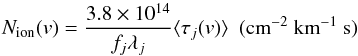 (A.1)where fj, λj and ⟨
τj(v)
⟩ are respectively the oscillator strength, the rest wavelength and
the average optical depth across the emission source of the line j for which the optical
depth solution is derived (see Edmonds et al.
2011). The optical depth solution across a trough is found for a given ion by
assuming an absorber model. As shown in Edmonds et al.
(2011), the major uncertainty on the derived column-densities comes from the
choice of absorption model. In this study we investigate the outflow properties using
column-densities derived from three common absorber models.
(A.1)where fj, λj and ⟨
τj(v)
⟩ are respectively the oscillator strength, the rest wavelength and
the average optical depth across the emission source of the line j for which the optical
depth solution is derived (see Edmonds et al.
2011). The optical depth solution across a trough is found for a given ion by
assuming an absorber model. As shown in Edmonds et al.
(2011), the major uncertainty on the derived column-densities comes from the
choice of absorption model. In this study we investigate the outflow properties using
column-densities derived from three common absorber models.
Assuming a single, homogeneous emission source of intensity F0, the simplest absorber model is the one where a homogeneous absorber parameterized by a single optical depth fully covers the photon source. In that case, known as the apparent optical depth scenario (AOD), the optical depth of a line j as a function of the radial velocity v in the trough is simply derived by the inversion of the Beer-Lambert law: τj(v) = −ln(Fj(v) /F0(v)), where Fj(v) is the observed intensity of the line.
Early studies of AGN outflows pointed out the inadequacy of such an absorber model, specifically its inability to account for the observed departure of measured optical depth ratio between the components of typical doublet lines from the expected laboratory line strength ratio R = λifi/λjfj. Two parameter absorber models have been developed to explain such discrepancies.
Observations and flux values for all epochs.
The partial covering model (e.g. Hamann et al.
1997; Arav et al. 1999, 2002, 2005)
assumes that only a fraction C of the emission source is covered by absorbing
material with constant optical depth τ. In that case, the intensity observed for a
line j of a
chosen ion can be expressed as ![]() (A.2)Our third choice are inhomogeneous absorber
models. In that scenario, the emission source is totally covered by a smooth
distribution of absorbing material across its spatial dimension x. Assuming the typical
power law distribution of the optical depth τ(x) =
τmaxxa
(de Kool et al. 2002; Arav et al. 2005, 2008), the
observed intensity observed for a line j of a chosen ion is given by
(A.2)Our third choice are inhomogeneous absorber
models. In that scenario, the emission source is totally covered by a smooth
distribution of absorbing material across its spatial dimension x. Assuming the typical
power law distribution of the optical depth τ(x) =
τmaxxa
(de Kool et al. 2002; Arav et al. 2005, 2008), the
observed intensity observed for a line j of a chosen ion is given by 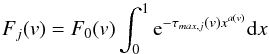 (A.3)Once the line profiles have been binned on
a common velocity scale (we choose a resolution dv = 20 km s-1,
slightly lower than the resolution of COS), a velocity dependent solution can be
obtained for the couple of parameters (C,τj)
or (a,τmax) of both
absorber models as long as one observes at least two lines from a given ion, sharing the
same lower energy level. Once the velocity dependent solution is computed, the
corresponding column density is derived using Eq. (A.1) where ⟨
τj(v) ⟩ =
Cion(v)τj(v)
for the partial covering model and ⟨
τj(v) ⟩ =
τmax,j(v) /
(aion(v) + 1) for the
power law distribution. Note that the AOD solution can be computed for any line (singlet
or multiplet), without further assumption on the model, but will essentially give a
lower limit on the column-density when the expected line strength ratio observed is
different from the laboratory value.
(A.3)Once the line profiles have been binned on
a common velocity scale (we choose a resolution dv = 20 km s-1,
slightly lower than the resolution of COS), a velocity dependent solution can be
obtained for the couple of parameters (C,τj)
or (a,τmax) of both
absorber models as long as one observes at least two lines from a given ion, sharing the
same lower energy level. Once the velocity dependent solution is computed, the
corresponding column density is derived using Eq. (A.1) where ⟨
τj(v) ⟩ =
Cion(v)τj(v)
for the partial covering model and ⟨
τj(v) ⟩ =
τmax,j(v) /
(aion(v) + 1) for the
power law distribution. Note that the AOD solution can be computed for any line (singlet
or multiplet), without further assumption on the model, but will essentially give a
lower limit on the column-density when the expected line strength ratio observed is
different from the laboratory value.
UV column-densities for the outflow components in NGC 5548.
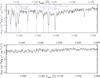 |
Fig. A.1
2013 spectrum of NGC 5548. The vertical axis is the flux in units of 10-14 erg s-1 cm-2 Å-1, and the quasar-rest-frame and observer-frame wavelengths are given in Angstroms on the top and bottom of each sub-plot, respectively. Each of the six kinematic components of the outflow shows absorption troughs from several ions. We place a vertical mark at the expected center of each absorption trough (following the velocity template of Si iv and N v) and state the ion, rest-wavelength and component number (C1–C6). We also assign a color to each component number that ranges from blue (C1) to red (C6). Absorption lines from the ISM are likewise marked in black with dashed lines. |
| Open with DEXTER | |
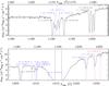 |
Fig. A.1
continued. |
| Open with DEXTER | |
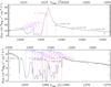 |
Fig. A.1
continued. |
| Open with DEXTER | |
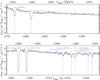 |
Fig. A.1
continued. |
| Open with DEXTER | |
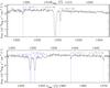 |
Fig. A.1
continued. |
| Open with DEXTER | |
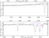 |
Fig. A.1
continued. |
| Open with DEXTER | |
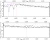 |
Fig. A.1
continued. |
| Open with DEXTER | |
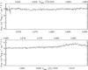 |
Fig. A.1
continued. |
| Open with DEXTER | |
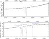 |
Fig. A.1
continued. |
| Open with DEXTER | |
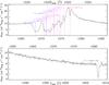 |
Fig. A.1
continued. |
| Open with DEXTER | |
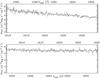 |
Fig. A.1
continued. |
| Open with DEXTER | |
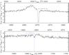 |
Fig. A.1
continued. |
| Open with DEXTER | |
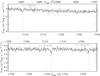 |
Fig. A.1
continued. |
| Open with DEXTER | |
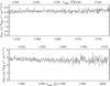 |
Fig. A.1
continued. |
| Open with DEXTER | |
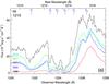 |
Fig. A.2
Spectrum of NGC 5548 during the five epochs of observation. The 2013 spectrum is obtained by co-adding visits 1 through 5. Spectral regions where absorption troughs from five ions are shown in sub-plots a) through e) and the six kinematic components associated with such absorption are labelled C1 through C6. |
| Open with DEXTER | |
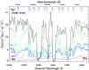 |
Fig. A.2
continued. |
| Open with DEXTER | |
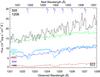 |
Fig. A.2
continued. |
| Open with DEXTER | |
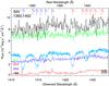 |
Fig. A.2
continued. |
| Open with DEXTER | |
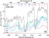 |
Fig. A.2
continued. |
| Open with DEXTER | |
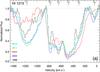 |
Fig. A.3
Normalized spectrum of NGC 5548 during the five epochs of observation, plotted in the velocity rest-frame of the quasar (same annotation as Fig. A.2). |
| Open with DEXTER | |
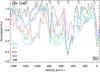 |
Fig. A.3
continued. |
| Open with DEXTER | |
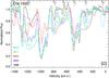 |
Fig. A.3
continued. |
| Open with DEXTER | |
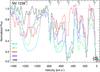 |
Fig. A.3
continued. |
| Open with DEXTER | |
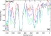 |
Fig. A.3
continued. |
| Open with DEXTER | |
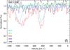 |
Fig. A.3
continued. |
| Open with DEXTER | |
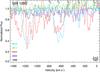 |
Fig. A.3
continued. |
| Open with DEXTER | |
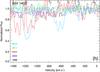 |
Fig. A.3
continued. |
| Open with DEXTER | |
© ESO, 2015
Current usage metrics show cumulative count of Article Views (full-text article views including HTML views, PDF and ePub downloads, according to the available data) and Abstracts Views on Vision4Press platform.
Data correspond to usage on the plateform after 2015. The current usage metrics is available 48-96 hours after online publication and is updated daily on week days.
Initial download of the metrics may take a while.