| Issue |
A&A
Volume 566, June 2014
|
|
|---|---|---|
| Article Number | A53 | |
| Number of page(s) | 36 | |
| Section | Extragalactic astronomy | |
| DOI | https://doi.org/10.1051/0004-6361/201323310 | |
| Published online | 11 June 2014 | |
Rapidly growing black holes and host galaxies in the distant Universe from the Herschel Radio Galaxy Evolution Project ⋆,⋆⋆
1 European Southern Observatory, Karl Schwarzschild Straße 2, 85748 Garching bei München, Germany
2 Institut d’Astrophysique de Paris, 98bis boulevard Arago, 75014 Paris, France
3 CSIRO Astronomy & Space Science, PO Box 76, Epping, NSW 1710, Australia
4 Department of Earth and Space Science, Chalmers University of Technology, Onsala Space Observatory, 43992 Onsala, Sweden
e-mail: guidro@chalmers.se
5 Kapteyn Astronomical Institute, Univ. of Groningen, Netherlands
6 Instituto de Astrofísica, Facultad de Física, Pontificia Universidad Catlica de Chile, 306, Casilla 306 Santiago 22, Chile
7 Space Science Institute, 4750 Walnut Street, Suite 205, Boulder, Colorado 80301, USA
8 Instituto de Física y Astronomía. Universidad de Valparaíso, Avda. Gran Bretaña 1111, Valparaíso, Chile
9 INAF – Osservatorio di Roma, via Frascati 33, 00040 Monteporzio, Italy
10 Astronomisches Institut, Ruhr-Universität Bochum, Universitätstr. 150, 44801 Bochum, Germany
11 School of Physics and Astronomy, University of Nottingham, University Park, Nottingham, NG7 2RD, UK
12 Department of Physics, Durham University, South Road, Durham, DH1 3LE, UK
13 Institut d’Astrophysique Spatiale, CNRS, Université Paris-Sud, 91405 Orsay, France
14 Leiden Observatory, University of Leiden, PO Box 9513, 2300 RA Leiden, The Netherlands
15 Jet Propulsion Laboratory, California Institute of Technology, Mail Stop 169-221, Pasadena, CA 91109, USA
Received: 20 December 2013
Accepted: 28 March 2014
We present results from a comprehensive survey of 70 radio galaxies at redshifts 1 <z< 5.2 using the PACS and SPIRE instruments on board the Herschel Space Observatory. Combined with existing mid-IR photometry from the Spitzer Space Telescope, published 870 μm photometry, and new observations obtained with LABOCA on the APEX telescope, the spectral energy distributions (SEDs) of galaxies in our sample are continuously covered across 3.6–870 μm. The total 8–1000 μm restframe infrared luminosities of these radio galaxies are such that almost all of them are either ultra-(LtotIR 1012 L⊙) or hyper-luminous (LtotIR 1013 L⊙) infrared galaxies. We fit the infrared SEDs with a set of empirical templates which represent dust heated by a variety of starbursts (SB) and by an active galactic nucleus (AGN). We find that the SEDs of radio galaxies require the dust to be heated by both AGN and SB, but the luminosities of these two components are not strongly correlated. Assuming empirical relations and simple physical assumptions, we calculate the star formation rate (SFR), the black hole mass accretion rate (ṀBH), and the black hole mass (MBH) for each radio galaxy. We find that the host galaxies and their black holes are growing extremely rapidly, having SFR ≈ 100–5000 M⊙ yr-1 and ṀBH ≈ 1–100 M⊙ yr-1. The mean specific SFRs (sSFR) of radio galaxies at z> 2.5 are higher than the sSFR of typical star forming galaxies over the same redshift range, but are similar or perhaps lower than the galaxy population for radio galaxies at z< 2.5. By comparing the sSFR and the specific ṀBH (sṀBH), we conclude that black holes in radio loud AGN are already, or soon will be, overly massive compared to their host galaxies in terms of expectations from the local MBH–MGal relation. In order to catch up with the black hole, the galaxies require about an order of magnitude more time to grow in mass at the observed SFRs compared to the time the black hole is actively accreting. However, during the current cycle of activity, we argue that this catching up is likely to be difficult because of the short gas depletion times. Finally, we speculate on how the host galaxies might grow sufficiently in stellar mass to ultimately fall onto the local MBH–MGal relation.
Key words: galaxies: active / quasars: general / galaxies: high-redshift / galaxies: evolution / quasars: supermassive black holes / infrared: galaxies
Herschel is an ESA space observatory with science instruments provided by European-led Principal Investigator consortia and with important participation from NASA.
Tables 2–4, 6 and Appendices are available in electronic form at http://www.aanda.org
© ESO, 2014
1. Introduction
At high-redshifts, deep submm observations suggest that massive galaxies have high flux densities and vigorous, on-going star formation (e.g. Hughes et al. 1998; Barger et al. 1998; Stevens et al. 2003; Chapman et al. 2005; Wardlow et al. 2011; Swinbank et al. 2014). The sensitivity of wide-field bolometer arrays limits these studies to only the brightest submm emitters (e.g. Weiß et al. 2009). Such bright submm galaxies (SMGs) frequently appear to be highly disturbed, which favours gas inflows driven by mergers as the chief instigator for generating the high observed submm fluxes (e.g. Somerville et al. 2001; Engel et al. 2010). Whether these intense starbursts are driven by mergers or by high rates of cold gas accretion is a question that is still actively debated (e.g. Noeske et al. 2007; Daddi et al. 2007; Tacconi et al. 2008).
Often, vigorous star formation is accompanied by powerful active galactic nuclei (AGN; e.g. Hopkins & Quataert 2010; Wang et al. 2011; Seymour et al. 2012; Rosario et al. 2012). The presence of AGN is revealed throughout the electromagnetic spectrum, from X-rays to radio, and in both continuum and line emission (e.g. Carilli et al. 1997; Hardcastle & Worrall 1999; Vernet et al. 2001; Alexander et al. 2005; Ogle et al. 2006; Nesvadba et al. 2008; Ivison et al. 2012; Wang et al. 2013). How AGN are triggered remains one of the most challenging questions of contemporary extragalactic astrophysics (for a recent review see Alexander & Hickox 2012). Even if current solutions and simulations are not completely satisfying (e.g. Hopkins & Quataert 2010), it is evident that the same material, cold molecular gas, is the reservoir out of which stars are formed and the AGN is fuelled (e.g. Hicks et al. 2009).
Interestingly, the expected correlation between AGN activity and star formation rate (SFR) is not obvious in observations, both locally and at high-redshift (e.g. Netzer 2009; Hatziminaoglou et al. 2010; Asmus et al. 2011; Dicken et al.(2012)Dicken Tadhunter; Bongiorno et al. 2012; Harrison et al. 2012; Rosario et al. 2012, 2013; Feltre et al. 2013; Videla et al. 2013; Esquej et al. 2014; Leipski et al. 2014). This may be due to high variability of AGN (Hickox et al. 2011) or the differences in timescales it takes for gas to become unstable, collapse to form stars over kpc scales compared to the time it takes for gas to lose sufficient angular momentum to reach the inner central parsec of the galaxy (Jogee et al. 2005). Despite our difficulties in understanding how relationships between the host galaxy and supermassive black holes come about, we observe a tight correlation between the black hole and the physical properties of their host galaxies in the local universe (e.g. Magorrian et al. 1998; Gebhardt et al. 2000; Ferrarese & Merritt 2000; Häring & Rix 2004). These relations suggest that both components of galaxies grew simultaneously (e.g. Hopkins et al. 2006). Nevertheless, some discrepancies have been observed from the local relation implying either an observational bias or a possible evolution of this relation with redshift (e.g. Lauer et al. 2007; Zhang et al. 2012). Currently, there are no complete answers that reconcile all the observations (Kormendy & Ho 2013, for a recent review).
Observations of infrared emission plays a crucial role in disentangling the relative importance of star formation and AGN to the bolometric emission from galaxies. As the IR emission is a mixture of dust heated by both the stars and the AGN, the nature of the IR spectral energy distribution (SED) can be used to probe the relative growth of galaxies and supermassive black holes and how their growth rates are related (known as the AGN-starburst connection). The short cooling time of the dust provides us with a snapshot of the heating rate of a galaxy due to the re-emission of absorbed UV and optical photons (e.g. Draine 2003). However, the peak of the IR SED, where both heating of dust grains by AGN and star formation make important contributions, was not completely covered with good sensitivity by Spitzer or by ground-based submm photometry for distant galaxies (e.g. Archibald et al. 2001; Reuland et al. 2004; Cleary et al. 2007; De Breuck et al. 2010; Rawlings et al. 2013). Herschel now provides the first opportunity to explore the complete IR SED of high redshift AGN, and thus to examine the relative contribution of the AGN and star formation to the bolometric luminosity of galaxies over a wide range of redshift.
Powerful radio galaxies are crucial objects in understanding the evolution of massive galaxies. They present all phenomenology undergoing both active star formation and rapidly accreting supermassive black holes. Powerful radio jets, strong and highly ionised optical and near-IR emission lines, and luminous mid-IR continuum, for example, betray the presence of an accreting supermassive black hole (e.g. Carilli et al. 1997; Vernet et al. 2001; Nesvadba et al. 2008; De Breuck et al. 2010; Drouart et al. 2012; Rawlings et al. 2013). They also have luminous submm emission, which is directly related to their vigorous star formation. Moreover, they have elliptical light profiles (Matthews et al. 1964; van Breugel et al. 1998; Pentericci et al. 1999; Zirm et al. 2003), are extremely massive (Rocca-Volmerange et al. 2004; Seymour et al. 2007), and are often associated with high density environments (e.g. Venemans et al. 2007; Falder et al. 2010; Hatch et al. 2011; Kuiper et al. 2011; Galametz et al. 2012; Wylezalek et al. 2013a). In other words, they have many hallmarks of a massive (perhaps cluster) galaxy in formation (Miley & De Breuck 2008).
Main parameters of the Herschel bands and photometry for isolated sources.
By their fortuitous edge-on orientation, the radio galaxies present a dusty torus occulting the light from the hot accretion disc (Type 2 AGN), enabling the simultaneous study of the host galaxy and the AGN, more easily than in the case of quasars (i.e. Type 1 AGN, for a recent review, see Antonucci 2012). Therefore, observing and characterising the different constituents of high-redshift radio galaxies appears to be our best chance to gain insights on the connection of the galaxy and black hole growth at much earlier stage in their history, more especially during the peak of the cosmic AGN and star formation activity (Hopkins & Beacom 2006; Aird et al. 2010). Since characterising the host galaxy/BH through dynamic properties at high-redshift is observationally expensive (Nesvadba et al. 2011), and beyond the reach of most of the current facilities, one has to rely on energetic diagnostics (such as SED decomposition) and empirical relations (Ferrarese & Merritt 2000; Häring & Rix 2004; Merloni et al. 2010, e.g. MBH-σ, MBH–Mbulge, MBH–MK) to investigate this (non-)relation during the first half of the history of the Universe in larger samples.
In this paper, we analyse the characteristics of the IR SEDs of a sample of 70 powerful radio galaxies spanning the redshift range from 1 to 5.2. This large sample allows us to compare the properties of the IR SED with their other characteristics (e.g. radio luminosities and sizes). The paper is organised as follows: Sect. 2 outlines the Herschel and submm observations and data reduction; Sect. 3 demonstrates how the photometry was calculated in cases of isolated and blended sources in the Herschel images; Sect. 4 discusses the IR luminosities and the SED fitting procedure which was used to estimate the bolometric, AGN and starburst luminosities; Sect. 5 compares the IR emission with other properties of the radio galaxies; and Sect. 6 discusses the interpretation of these luminosities in terms of physical parameters allowing us to put new constraints on the evolution of radio galaxies. Throughout this paper, we adopt the concordance cosmological model (H0 = 70 km s-1 Mpc-1, ΩΛ = 0.7, ΩM = 0.3).
2. Observations and data reduction
This paper aims to disentangle the IR SED of a sample of 70 powerful radio galaxies spanning the redshift range 1–5.2. This HErschel Radio Galaxies Evolution (HeRGÉ) sample is identical to the Spitzer High-z Radio Galaxies (SHzRG) sample described by Seymour et al. (2007) and De Breuck et al. (2010). We briefly summarise here the criteria selected to build this sample. The radio galaxies have been selected to cover homogeneously the radio luminosity-redshift plane, applying the criteria L3 GHz> 1026 WHz-1, where L3 GHz is the total luminosity at a rest-frame frequency of 3 GHz (Table 1; Seymour et al. 2007).
We first describe the new Herschel data of our entire sample, followed by a presentation of submm data which were obtained with the LArge Bolometer CAmera (LABOCA) on the APEX telescope to complete the submm observations of our sample1.
2.1. Herschel far-IR data
The far-IR data for all 70 sources were obtained with the Herschel Space Observatory (Pilbratt et al. 2010) in five broadbands: in two bands with PACS (Photodetector Array Camera and Spectrometer; Poglitsch et al. 2010, at 160 μm and either 70 μm or 100 μm depending on the redshift of the radio galaxy) and in three bands with SPIRE (Spectral and Photometric Imaging REceiver; Griffin et al. 2010, at 250, 350, and 500 μm). Our programme was observed between 2011 February and 2012 March. Several sources were already observed as part of guaranteed time observations, and those data were obtained from the Herschel Science Archive (see Table 2 for program and ObsID).
2.1.1. PACS reduction
The PACS instrument covers the spectral region from 60 μm to 210 μm. The mini-scan map mode was used on each science target, using the PACS (70 μm)/PACS (160 μm) and PACS (100 μm)/PACS (160 μm) configurations for sources at z< 2 and z> 2, respectively. Each observation consisted of two cross-scan images centred on the source. The final map covers about 2 × 4 arcmin, with homogeneous coverage of 50 arcsec diameter around the target. The observations of PKS 1138-262 cover a larger field, but were reduced using the same procedure. As each PACS observation consists of a simultaneous scan in two bands at medium scan speed (20 arcsec s-1), two subimages are produced for each band and co-added to obtain the final maps. Each data set was reduced from level 0 using the Herschel interactive processing environment, version 8 (HIPE; Ott 2010) using the standard deep miniscan pipeline. As we are looking for faint sources, the MMTDeglitching task was applied on level 0.5 of the data and we checked on the coverage map that no flux was potentially removed from the source. The PACS data is dominated by 1/f noise, so we applied a high-pass filter on level 1 data with a high-pass filtering radius (hpfradius) value of 15 readouts for the blue/green channel and 25 readouts for the red channel with a circular mask of 15 arcsec radius centred on the galaxy coordinates (best strategy available, see Popesso et al. 2012). Finally, each map was projected onto a user-defined world coordinate system (WCS) grid centred on the source. As our observations have a high redundancy, we chose a small pixfraction value (0.01) and set the pixsize to the recommended values: 2 arcsec for the blue/green channel and 3 arcsec for the red channel (Table 1)2. Finally, the two submaps were co-added into a final map with the MosaicTask.
2.1.2. SPIRE reduction
The SPIRE instrument covers the spectral region in the range 200–700 μm. Each observation with SPIRE consists of three successive scans centred on the source with all three bands (250, 350, and 500 μm) at 30 arcsec s-1 scan speed. The only exception is again PKS 1138-262 which had four scans over a wider area. The final map for each source covers 8 × 10 arcmin, with a homogeneous exposure level throughout the entire field. We reduced the data with the Photometer small map pipeline within version 8 of HIPE. As glitches are present in the SPIRE timeline, several deglitching procedures were applied to the level 1 data. We choose the linearadaptive20 option for the wavelet deglitcher with all the other options at their default values. We used the naivemapmaker to create the final map with pixel sizes of 6, 10, and 14 arcsec for the maps at 250, 350, and 500 μm maps, respectively (Table 1).
2.2. Herschel photometry
Thanks to high-resolution radio observations (Carilli et al. 1997; Pentericci et al. 2000; De Breuck et al. 2010), radio galaxy positions are known to subarcsec accuracy. As the average Herschel pointing uncertainties are ~1 arcsec, we performed fixed aperture photometry directly on the known position of each radio galaxy. Because of the depth of the images and the large beam of Herschel, the aperture photometry is often contaminated by nearby companions, which may contribute significantly to the estimated flux of the radio galaxy. In order to estimate this contamination, we visually checked each galaxy in six bands, from MIPS (24 μm) to SPIRE (500 μm). As the 24 μm image provides the best spatial resolution with which to investigate the dust emission, it was used to isolate potential companions contributing to the total flux in the Herschel data. The SPIRE (250 μm) image, since it is taken through one of the most sensitive channels and has reasonable resolution, was used to provide long wavelength information about possible contaminated sources. We first mark all the positions of detected sources in the 24 μm image onto the Herschel maps. When a possible contaminating source was found within 60 arcsec, it was deblended to remove its contribution from the radio galaxy flux (see Sect. 2.2.2). Otherwise, a single aperture was used to estimate the flux (Table 3).
2.2.1. Isolated sources
When the image does not show a contamination in the MIPS (24 μm) and SPIRE (250 μm) images, aperture photometry was performed using the AnnularSkyAperturePhotomery task within HIPE. For a comparison between the different strategies, we refer to Popesso et al. (2012) and Pearson et al. (2013) for PACS and SPIRE, respectively. We summarise here briefly for our sample. For PACS, the best strategy of masking is applied (see Sect. 2.1.1), and aperture and point spread function (PSF) photometry gives similar results. For SPIRE, as our sample contains mainly faint sources (Fgal< 30 mJy), automatic procedures would normally be preferred (SUSSEXtractor or DAOphot). However, as our sample is subject to blending effects (see next section), PSF-photometry is mainly performed to measure source flux making use of Starfinder (similar to SUSSEXtractor). See Table 1 for a summary of the parameters. Table 3 reports the final flux, obtained after aperture correction in the case of aperture photometry.
2.2.2. Blended sources
Blending becomes more important, particularly for the SPIRE bandpasses where the large beams encompass a large area around the radio galaxy (for example, the SPIRE 500 μm beam corresponds to ~300 kpc at z = 1). While this is particularly problematic for blind source extraction at a single wavelength (Nguyen et al. 2010), we can use here the prior information given by higher resolution observations such as MIPS (24 μm) images.
We use Starfinder, software optimised for crowded fields, performing PSF photometry to estimate the fluxes of sources that are blended (Diolaiti et al. 2000). StarFinder requires both the estimated position of each source and the characteristics of the PSF. We defined a 2D Gaussian PSF with the FWHM equal to the beam size. Even if the PACS and SPIRE beams are slightly different from Gaussian, the energy in the secondary lobes is only a small fraction of the total integrated energy, and the Gaussian approximation is still valid. We checked this difference in the SPIRE images where several sources can be used to estimate the PSF. We found the differences to be negligible.
Even with input positions on possible sources, sometimes Starfinder did not converge on a solution, especially in the case where two sources are separated by less than the FWHM of the PSF for SPIRE. The SPIRE 500 μm band, which has the largest beam, is the most affected by this effect. For sources that could not be accurately deblended, we assume the total flux to be the upper limit for the radio galaxy.
The main caveat to this technique is the assumption that a source detected in SPIRE has a counterpart in the MIPS images. Using the average sensitivity of our MIPS (24 μm) and SPIRE (250 μm) images, we calculate the corresponding colour limit, log (F250 μm/F24 μm) = 2.12. Making use of templates from DecompIR (see Sect. 4), we find that this approach can miss some sources at z> 3 given our achieved sensitivities. Nevertheless, this contamination is estimated to be only a few percent (Roseboom et al. 2010; Magdis et al. 2011) and is therefore not taken into account for the remainder of this paper.
2.2.3. Uncertainties
The design of the PACS detectors makes these data prone to correlated noise (Popesso et al. 2012). While a formal estimate of this noise is almost impossible, it is possible to estimate the average total noise from the images. Given the observing strategy, we focused on the most homogeneous, central part of the images to estimate the noise. We drew identical, non-overlapping apertures around the source in a hexagonal pattern, and performed the same aperture photometry as used to estimate the flux of the central source. We considered the total noise on the map to be the standard deviation of these distributed apertures around the source.
For the SPIRE images, the uncertainties are calculated either in the sky annulus for the aperture photometry in the case of an isolated source, or by the standard deviation of the pixel value distribution of the map for the PSF-photometry.
2.3. Final uncertainty and Herschel flux
As the observations are centred at the position of the radio galaxies, which are well detected at shorter wavelength, we have a strong prior on the detection of a source at a given position. We define “strict non-detection”, “tentative detection”, and “strong detection” as sources detected at the Fgal< 2σ, 2σ<Fgal< 3σ, and Fgal> 3σ levels, respectively.
In the case of a non-detection (Fgal< 2σ), we took the upper limit as three times the sky standard deviation (we discussed the estimation of the uncertainties in previous sections). In the case of tentative detection (2σ<Fgal< 3σ), we provide the value of the flux between square brackets (Table 3) and display these as open diamonds on the SED plots (Fig. D.1). In addition, we add the calibration uncertainty in the formal errors for detected sources. Table 3 presents the final flux estimates and their associated total uncertainties (photon, instrumental, and confusion noise). They are calculated by adding quadratically the absolute calibration uncertainty (see Table 2) with the uncertainty estimated directly from the noise characteristics of the images (Sect. 2.2.3). Because of the additional flux calibration uncertainty, the signal-to-noise ratio does not correspond to the flux uncertainties given in Table 3, as these are calculated before applying the calibration correction.
2.4. LABOCA, submm data
In addition to the fluxes already available in the literature (Archibald et al. 2001; Reuland et al. 2003), we obtained new submm data for some of those sources lacking it3. We observed 18 sources in the southern hemisphere spanning 1 <z< 3. The observations were done in service mode between 2012 July and December, with precipitable water vapour generally below 1 mm. To save observing time, most sources were observed using the LABOCA wobbler on-off (WOO) photometry mode. As this WOO mode does not provide any spatial information, it should only be used on isolated sources. If the Herschel maps showed either multiple point-like sources within a radius of 20′′ (one LABOCA beam size), or a spatial offset more than 5′′ from the radio core position, we used the raster spiral mapping mode instead. The integration times per source were adapted to obtain an approximately uniform rms for all 18 sources. To reduce the data, we used the doOO script inside BoA (Schuller 2012) for the WOO data, and the reduction macro in CRUSH2 (Kovács 2008) for the mapping data. Table 4 summarises the observing modes, fluxes, uncertainties, and the references for data taken from the literature.
3. The HeRGÉ infrared spectral energy distributions
Combining the Spitzer, Herschel, and submm data, we continuously cover the wavelength range 16–870 μm. The panels in Fig. D.1 show the resulting SEDs for our 70 radio galaxies. As our focus is on the warm to cold dust emission, we do not use Spitzer IRAC photometry in our SEDs because those data are generally dominated by stellar photospheric emission (e.g. Seymour et al. 2007). De Breuck et al. (2010) show that hot dust emission can also contribute significantly to the IRAC fluxes of some sources. This hot dust component (>500 K), however, only represents a small fraction of energy of the total IR SED (<5%), and is influenced by orientation-dependent effects (Drouart et al. 2012). We therefore do not include this hot dust contribution in our SED fitting. Moreover, we add 20% uncertainties to the MIPS data to account for cross-calibration uncertainties between Spitzer and Herschel. We overplot the Spitzer spectrum available for a subsample of our sources (Seymour et al. 2008; Rawlings et al. 2013). These spectra are not used to constrain our fits, but provide a consistency check on our decomposition of the IR/submm SEDs.
3.1. Total IR luminosities
Since our IR/submm SEDs are well sampled, we can estimate robustly the total IR luminosity ( ). We use its most common definition, integrating the flux density in the 8–1000 μm restframe range. To interpolate between our photometric data points, we assume the models described in Sect. 4. From these estimates of the total IR luminosity, it appears that almost all radio galaxies from our sample are ultra-luminous infrared galaxies (ULIRG;
  > 1012L⊙).
Figure 1 plots our sample along with other samples available in the literature with Herschel observations. Our galaxies are among the brightest emitters in the IR in their redshift range. About half of our z> 2 sample belongs to the HyLIRG regime ( > 1013L⊙). From this diagram, it is interesting to note that the high-redshift radio galaxies are indistinguishable from the most extreme IR emitters.
Interestingly, such luminous objects imply strong AGN and/or star formation activities. This should be compared with previous results about the mass of these objects, located at the high-mass end of the galaxy mass distribution (e.g. Rocca-Volmerange et al. 2004; Seymour et al. 2007). Even if these galaxies are identified as the progenitors of the red-and-dead local ellipticals (e.g. Matthews et al. 1964; Rocca-Volmerange et al. 2004; Thomas et al. 2005; Labbé et al. 2005), they appear to be fairly active in the past.
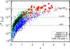 |
Fig. 1 Total IR luminosity ( |
3.2. The warm and cold dust contributions
While both AGN and SB can heat dust, their input SEDs are significantly different; AGN heating tends to contribute at shorter wavelengths (~10 μm,  K), whereas star formation heating tends to dominate the emission at longer wavelengths (~100 μm,
  K). Given the large variety of the data quality, we want to define a set of criteria to disentangle the AGN and SB contributions. We therefore classify our galaxies into classes depending on the number of detections on either side of 50 μm restframe (e.g. Leipski et al. 2013). This value is preferred for several reasons. First, in the case of an object with both contributions (AGN and SB), the change in regime is expected to occur around this wavelength. Second, our sample spans a large range in redshift (1 <z< 5) and therefore a simple colour selection would be severely affected by the k-correction. Third, this wavelength equally splits the number of channels available for each source (four bands on either side). We note that by changing this limit to 30 μm or 70 μm only changes the fraction of sources in each class by a small amount (<5%).
The classes are defined as follows, with their respective fractions in our sample:
-
1.
Warm and cold dust (WCD, 45%): corresponds to detections onboth sides of λrest = 50 μm.
-
2.
Warm dust (WD, 33%): corresponds to detections only in the mid-IR (λrest< 50 μm).
-
3.
Cold dust (CD, 11%): corresponds to detections only in the far-IR (λrest> 50 μm).
-
4.
Upper Limit (UL, 11%): corresponds to no detections in either the mid-IR or the far-IR.
We detect warm, preferentially AGN-heated dust emission in most (78%) of our sample, while the cooler, preferentially starburst-heated dust emission is detected in half (54%) of our sample (Table 6). This difference between the possible constraints on the two components can be interpreted in two ways: either our Herschel (and in particular SPIRE) data are comparatively less sensitive than Spitzer, or the AGN contributes more significantly to the IR SED while the strength of the associated SB varies by a larger amount. We note that only 11% of our sample does not have any constraints on the relative contributions of either AGN or starbursts to the IR SED.
To further examine correlations involving IR luminosities in our sample, we next separate the AGN and SB components.
4. IR SED decomposition method
In order to decompose the two main contributions to the IR SED, AGN, and SB emission, we need models for each component. The AGN dust emission, which contributes mainly in mid-IR emission, comes mainly from the far-UV through optical light that has been reprocessed by dust in close proximity to the AGN. The far-UV through optical emission from any young stellar population that may exist is largely reprocessed into the far-IR via dust grains.
One of the most important goals of this analysis is to determine the relative emission from the AGN and starburst components. Disentangling this relative emission allows us to investigate the principal physical processes responsible for the luminous IR emission in distant radio galaxies, since the dust reprocessed emission is the largest contributor in active galaxies. This analysis provides the best measure of the bolometric luminosity.
We use the SED fitting procedure DecompIR (Mullaney et al. 2011, https://sites.google.com/site/decompir/home), with some minor modifications to add the information and constraints provided by the Herschel and submm data. Briefly, DecompIR allows the fitting of one or two templates thanks to χ2 minimisation. It considers an empirical library estimated from local starburst and an empirical unique AGN template consisting of a composite spectrum of broken power-laws and a black body. All templates cover the 3–1000 μm restframe range4, and an extinction can be applied independently for each component. This procedure has been extensively tested on higher redshift sources and described in Del Moro et al. (2013). In order to keep our approach as homogeneous as possible over the whole sample, we minimise the number of free parameters. We remind the reader that we did not include the IRAC data because it contains a significant component of stellar photospheric emission.
4.1. Additional starburst template
DecompIR includes five different SB templates. Briefly, they represent SB with different peaking temperatures and polycyclic aromatic hydrocarbon (PAH) strength, with the coldest corresponding to SB1. We refer to Mullaney et al. (2011,their Fig. 4) for presentation of the SEDs. For two galaxies (4C 41.17 and 4C 28.58), these five available templates do not converge to an acceptable solution. The best fitting SED suggests that either a hotter starburst component or a colder AGN contribution (Fig. D.1) is required to reproduce the observed SED. However, 4C 41.17 is well fitted by a synthetic SED from the galaxy synthesis and evolution code, PEGASE.3 (Rocca-Volmerange et al. 2013). Fortuitously, this galaxy appears to have a relatively small AGN contribution (Dey et al. 1997). Rocca-Volmerange et al. (2013) show that the IR part of the SED is clearly dominated by a young stellar population. We have therefore included the IR part of the best fitting SED of 4C 41.17 from PEGASE.3 as a new template to the DecompIR library (the SB6 template). This template has the highest relative dust temperature of any of the SB templates in the library – its dust emission peaks at ~60 μm (~50 K). This template does not represent a local SB as the other templates do; it is a solution for a 30 Myr old starburst (Rocca-Volmerange et al. 2013). However, we seek here only to reproduce the general shape of the IR SED to estimate IR luminosities, and will not make any further considerations about the age/mass of this template. A further analysis of the SB/host properties similar to the approach Rocca-Volmerange et al. (2013) is the object of a forthcoming paper (Drouart et al., in prep.).
4.2. AGN template
The AGN template used in this analysis is calculated using a sample of AGN that has had the starburst contribution removed from their mid-IR SED. The template is an average of the residual mid-IR SEDs (see Mullaney et al. 2011, for details). Because of the empirical nature of this subtraction and the variety of possible AGN-dominated mid-IR SEDs, this average template is expected to show discrepancies from object to object; however it satisfactorily represents the average AGN spectrum in mid-IR (Dale et al. 2014). Ideally, we would like to use different AGN templates, similar to the SB analysis. In particular, the hottest part of the AGN is subject to inclination-dependent effects (e.g. Leipski et al. 2010; Drouart et al. 2012).
In order to test this, we modified DecompIR to include the average Type 1 AGN template from Richards et al. (2006) onto which we apply an extinction from Fitzpatrick (1999). Even if this AGN template significantly improves our fitting, we decided to discard this template from our library for the following reasons. First, the inclusion of an extra parameter (the extinction) decreases the number of sources on which our fitting can be applied. Second, the Richards template presents an odd and unrealistic tail in the far-IR (probably due to the poor far-IR coverage of the data set used to build this template). Third, while increasing the scatter in  , we find no drastically different results from using the built-in AGN template. Finally, being an average template, star formation can still contribute at long wavelength and we would therefore overestimate the AGN luminosity.
4.3. Transition regime: hot starburst or cold AGN?
The transition between the two components is the most critical parameter as it has an important influence on the calculated IR luminosities. On the one hand, we want to be sure that the templates we are using are effectively representative of the AGN and/or the SB components. On the other hand, we want to keep the decomposition as simple as possible to apply it over the entire sample. As previously mentioned, we use only one AGN template, deemed representative of the general AGN SED. How can we be certain that this empirical template is representative of all our sources? This question is difficult to answer as the data quality varies from object to object and we only have broadband photometry for our sample. Nevertheless, one can argue that this template is valid considering the following assumptions. The cold dust emission for the AGN (λrest> 30 μm) can come from (i) an extended torus (e.g. Fritz et al. 2006; Nenkova et al. 2008), or (ii) reprocessed light from the NLRs (e.g. Dicken et al. 2009, 2010). While (i) will require the inclusion of a large number of new free parameters; (ii) can only be assessed by the [OIII] luminosities that are not available for our entire sample. The quantification of these effects is beyond the scope of this paper and will therefore be ignored for the remainder of the analysis. Moreover, one notes that the empirical AGN template does present a significant contribution at long wavelength. It is also interesting to note that the extreme object 4C 23.56 represents the prototype of a pure AGN contribution, and is remarkably well reproduced by the built-in template. Part of our sample (seven objects) have IRS spectra (12–24 μm) available (Seymour et al. 2008; Rawlings et al. 2013). Overplotting the spectrum after the fitting shows a good agreement between the IRS and the results. Finally, the overall results do not seem to bias our results towards one or another SB template (see Table 6).
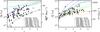 |
Fig. 2 Left: |

4.4. AGN/SB relative contribution
The relative contribution of the AGN and the SB can vary a lot, depending on the physical condition of the SB or the configuration of the dust close to the AGN (see previous section). In order to check this potential impact on the previously defined classification (UL, CD, WD, WCD) we define three values of the relative AGN and SB contribution to the flux at 10, 50, and 100 μm restframe ( ). This relative contribution may vary depending on the SB template used for the fit. In the mid-IR (10 μm), this effect can be strong due to the emission from PAH molecules. For the two extreme starburst templates, this relative contribution can vary by up to a factor of 4. Nevertheless, in most cases, we can discriminate between the most extreme templates (SB1 and SB5) which have a factor of ~2 difference in their relative contributions for the same total luminosity. In the far-IR (100 μm) this relative difference is smaller, the SB dominates the SED except for a few cases (e.g. 4C 23.56). Appendix B shows these fractions as a function of the total infrared luminosity .
4.5. Procedure on the sample
Distribution of the sample as a function of their class and their number of detections in the IR.
The large difference in data quality prevents us from blindly applying the same fitting procedure on all galaxies in the full sample. In order to take full advantage of our data, we apply different procedures on each source, depending on the number and the quality of detections, and their previously defined classes (see Sect. 3.2 and Table 5). We also highlight some special cases that need a specific treatment. We stress that independently from their designated class, each acceptable solution must respect the 3-sigma rule: if a solution presents a template brighter that any of our 3σ detection limits, this solution is discarded as not physically acceptable. We note that all calculated infrared luminosities are integrated over the 8–1000 μm range.
UL sources:
for sources without any firm detections, only upper limits on and  can be calculated. We normalise separately the AGN template and a SB template on the most constraining upper limit. The upper limit on is calculated by simultaneously fitting both templates on the most constraining upper limits.
WD sources:
for sources with detections only in the mid-IR, we fit only an AGN template. In a second step, we normalise a SB template to the most constraining upper limit in the far-IR. The upper limit on is calculated by simultaneously fitting both templates on the detected points in mid-IR and the most constraining upper limit in far-IR.
CD sources:
for sources with detections only in the far-IR, we fit only an SB template. If the number of detections allows it (n ≥ 2), we leave the type (SB1 to SB6) as a free parameter. In a second step we normalise the AGN template on the most constraining upper limit in the mid-IR. The upper limit on is calculated by simultaneously fitting both templates on the detected points in the far-IR and the most constraining upper limit in the mid-IR.
WCD sources:
for sources with two or three detections in the mid- and far-IR, we fit both AGN and SB components, but choose the SB template which maximises with respect to the most constraining upper limits in the far-IR. For sources with four or more detections, we fit both the AGN and SB components, with the SB type template as an additional free parameter in the fitting. In both cases, is the sum of both templates. As mentioned previously, extinction could have a strong impact on the fitting. We tested for this effect on this subsample adding the extinction as a free parameter on both components. The and are changed within a factor of <3. We therefore do not consider extinction in our fitting procedure for the reminder of this paper.
Table 6 provides the measured , , , and SB template given by the best solution and the AGN fraction at 10, 50, and 100 μm restframe. The AGN fractions are described in Sect. 4.4 and Appendix B.
5. Results
5.1. AGN/SB detection limits
Figure 2 shows both the infrared AGN and SB luminosities as a function of redshift. In order to verify whether the upper limits on the AGN and the SB components are mainly due to physical processes or purely from an observational bias, we calculate the minimum luminosity for each component related to the band sensitivity. Our 3σ sensitivity limits are calculated averaging the uncertainties over the entire sample. We normalise the AGN and SB35 templates in each observed band and calculate the corresponding or at any redshift.
One notes that our upper limits do not always follow the most sensitive detection limit (for instance the black line on left plot). This can be explained in several ways: (i) the IR emission is a mixture of AGN- and SB-heated dust; (ii) especially in the IR, the background emission varies locally and as a function of Galactic longitude, affecting the final sensitivity; or (iii) the depth of the MIPS (24 μm) imaging is not uniform throughout the sample (De Breuck et al. 2010).
From these diagrams, MIPS 24 μm data appear to be the most sensitive to the AGN contribution at any redshift. It is important to remember that a pure AGN contribution is very unlikely to be detected in the submm as they require AGN of > 1014 L⊙ at any redshift (see orange SCUBA line at the top of Fig. 2, left). Nevertheless, one should be careful to associate the 24 μm flux to the AGN because PAH contributions from star formation can be important in this band (see plateau in Fig. 2, right). In the case of a pure SB component, the situation is completely different. Up to z ~ 2, MIPS 24 μm is again our most sensitive band to detect both SB and AGN. However, in the case of a pure SB component, the SB will be detected only at > 1012 L⊙ where for the same sensitivity a pure AGN will be detected at the > 3 × 10¹¹ L⊙ level. This implies that the MIPS 24 μm band is likely to be dominated by AGN emission if any hints of AGN activity is detected in a source (which is the case for radio galaxies).
At z> 2, SCUBA (and LABOCA) become our most sensitive bands for detecting SB components. Moreover, due to k-correction effects (Blain et al. 1999), this limit is roughly constant with redshift. Our 3σ sensitivity allows us to detect starburst activity of at least 400 M⊙ yr-1 (800 M⊙ yr-1 for LABOCA) assuming the standard -SFR conversion law (Kennicutt 1998).
5.2. Infrared AGN and starburst luminosities
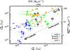 |
Fig. 3
|

Figure 2 plots and versus redshift. Both plots suggest an increasing trend with redshift (ρ = 0.374, p = 0.0019 and ρ = 0.613, p< 0.0001, respectively6). While this trend seems real for (given the few upper limits), it appears stronger with . Even if is affected by numerous upper limits, especially at z< 2.5 (due to the limited sensitivity of the 250 μm SPIRE band), these upper limits are fully consistent with an increasing trend. An improvement of one order of magnitude in our far-IR sensitivities should certainly be enough to detect the missing sources and therefore confirm the increasing trend with redshift for .
We also estimate the black hole accretion rate (ṀBH) and the SFR based on the fits to the SED. We discuss these parameters in greater detail in Sect. 6. First, we note that our sample spans a large range in both SFR and ṀBH, almost two orders of magnitude for both of them, 1 M⊙ yr-1 < ṀBH < 100 M⊙ yr-1 and 100 M⊙ yr-1 <SFR< 5000 M⊙ yr-1. Moreover, as they scale linearly with and , the suggested increasing trend with redshift applies to both the SFR and the black hole accretion rate. In particular, all our z< 2 sources have a ṀBH < 5 M⊙ yr-1, while at z> 2, ṀBH can reach 100 M⊙ yr-1. The same behaviour, although weaker, can be observed with SFR where all sources (except one) have SFR< 1000 M⊙ yr-1 at z< 2.5, while SFR can reach 4000 M⊙ yr-1 for the sources with the highest redshifts.
Figure 3 plots versus (we discuss this plot more extensively in Sect. 6). Radio galaxies cover a wide range of relative contributions: from almost pure star forming galaxies (e.g. 4C 41.17), to almost pure AGN contribution (e.g. 4C 23.567) but with the majority having SEDs which are composites of star formation and AGN heating (e.g. PKS 1138-262). We indicate these three specific sources in Fig. 3 as black crosses.
Taking into account only the objects with good constraints on both their AGN and SB contributions, we find no significant correlation. This provides confidence about the decomposition as we do not expect, a priori, to have a correlation between the AGN and SB luminosities (as also found in other studies, e.g. Bongiorno et al. 2012; Dicken et al.(2012)Dicken Tadhunter; Feltre et al. 2013; Leipski et al. 2014). Nevertheless, it is interesting to note that each component (AGN and SB) has an integrated luminosity of LIR> 1012 L⊙. This indicates that a high IR luminosity does not necessarily imply a high star formation rate or a strong AGN activity.
5.3. Comparing AGN and SB IR luminosities with radio properties
5.3.1. Radio luminosities
De Breuck et al. (2010) calculated the 500 MHz restframe luminosity for the entire sample. In the case of powerful radio galaxies, the radio emission is dominated by the AGN. The 500 MHz luminosity ( ) is an excellent proxy for estimating the energy injected by the AGN into the lobes of the radio galaxy8.
We see a weak correlation over 2 orders of magnitude in and (Fig. 4, ρ = 0.475, p = 0.0001). However, both and present a correlation with redshift. As we constrained for most of our sample and is well determined, we apply a partial correlation test9 in order to take this mutual dependence on redshift into account. This partial test severely degrades the correlation (R = 0.10) indicating that redshift is the determinant factor of this correlation. It is therefore impossible to conclude much about the correlation between the radio and the IR in radio galaxies (at least with this sample which spans a wide redshift range but <2 orders of magnitude in radio luminosity).
This apparent lack of correlation can be easily explained by comparing the timescales in the IR and radio to respond to changes in the energy output of the AGN. The dust heated by the AGN is likely to be circumnuclear given its emission temperature. Dust cools quickly and the timescale for the photons to stream through the nebula is relatively short. The radio emission, on the other hand, has a much longer response time to changes in the AGN output and the aging time of electrons is of the order of tens of Myr (Blundell et al. 1999), especially at low frequencies and considering shock re-energisation in the lobes themselves. In addition, it is not clear if the relative fraction of energy and emission in the radio and IR should be similar anyway.
The luminosities and also tend to present a positive weak correlation (ρ = 0.536 and p = 0.001 applying a survival analysis), similarly to and . The numerous upper limits and poor statistics make it even more difficult to conclude anything about this correlation. Moreover, as for , this correlation also seems mostly driven by redshifts effects.
5.3.2. Radio sizes
 |
Fig. 4
|
Spatially resolved radio observations can measure the distance between the core and the lobe (or lobe-lobe), providing useful information on the age of the radio phase assuming a simple ballistic trajectory for the ejected particules (Blundell et al. 1999). The radio size, las (Table 2 in De Breuck et al. 2010), corresponds to the largest extension in 1.4 GHz radio maps. As all our radio galaxies have a spectroscopically determined redshift, we calculate the projected size D sin (i) in kpc of the radio galaxy where D is the physical size of the galaxy and the sin (i) term refers to its projection onto the sky plane. A degeneracy appears here due to the inclination i of the radio galaxy. Nonetheless, this quantity is not expected to be important, as we are dealing with Type 2 AGN, i.e. mostly oriented in the plane of the sky (Drouart et al. 2012). The real size D will likely be at most 30% larger because of projection effects.
Figure 5 plots against the projected size D sin (i). Similar to , coloured points show a redshift effect in our data; the most compact AGN are at higher redshift. Radio sizes could also be affected by two effects: (i) it can depend on environment (e.g. Kaiser et al. 1997; Klamer et al. 2006; Bornancini et al. 2010; Ker et al. 2012); and (ii) our sample presents a weak selection bias in size, with larger objects located at lower redshift (see Fig. 5).
5.4. Comparing IR luminosity with stellar mass
Our sample benefits from stellar mass estimates thanks to Spitzer data. By fitting the 3.6–24 μm range with a sum of an elliptical template from PEGASE.2 (Fioc & Rocca-Volmerange 1997) and blackbodies at various temperatures, De Breuck et al. (2010) estimated reliable stellar masses for our sample, finding values of ~1011−12 M⊙. Although massive, our low dynamic range in mass prevents us from drawing any conclusion about possible correlations. However, it is interesting to note the large scatter in the AGN luminosity, over two orders of magnitude, but the relatively small scatter in Mstel (see Fig. 5 in De Breuck et al. 2010). Plotting Mstel against exhibits the same behaviour, with the range of being smaller given the larger number of upper limits. It is interesting to compare these masses and with SMGs at similar redshift. While the SFRs are similar (e.g. Archibald et al. 2001; Reuland et al. 2004; Engel et al. 2010; Sect. 6.1.1), our sample of radio galaxies appears more massive by a factor of 2–5 (De Breuck et al. 2010; Hainline et al. 2011; Michalowski et al. 2012; Simpson et al. 2013).
6. Discussion
Having disentangled the total IR luminosities of the star formation and AGN components in the SEDs, we can now estimate star formation rates (SFR), because we have stellar mass estimates (Mstel), the specific star formation rates (sSFR), the black hole accretion rates (ṀBH), Eddington ratios (λ), and the specific black hole growth rates (sṀBH). These estimates will allow us to characterise the evolutionary state of powerful radio galaxies, since we have a sample that spans a wide range of redshifts.
Are the host galaxies and their black holes co-evolving or is one of them outgrowing the other? Because it is difficult to provide reliable uncertainties for individual sources and parameters and undoubtedly our estimates suffer from systematic uncertainties, we will have to interpret these estimates as ensemble averages instead of focusing on individual measurements. With these insights, we will attempt to characterize the place of radio galaxies in the population of distant galaxies and what their future evolution might be within the context of their place in the ensemble population of galaxies.
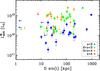 |
Fig. 5
|
6.1. How rapidly are radio galaxies and their black holes growing?
To put the radio galaxies into the context of the evolution of galaxies and into the broad range of black hole demographics (i.e. growth rate and masses), we need to convert estimates of the bolometric luminosities of both the recent star formation and the black hole accretion, and , into SFR and ṀBH. These estimates depend on the rate at which short wavelength emission (e.g. blue optical, UV) from young stars is reprocessed into the IR and submm and the rate at which the accreted mass onto the black hole is converted into radiated energy and the ratio of the IR luminosity to the total bolometric luminosity.
6.1.1. Star formation rate
We have found that powerful radio galaxies are extremely bright in the IR ( ), which may indicate that they have very high SFRs. We have seen in Sect. 5.2 that we can disentangle SB from AGN emission. We can thus provide much more reliable determinations of the SFR than previous submm only determinations (e.g. Archibald et al. 2001; Reuland et al. 2004). Given the high IR luminosities and the fact that we are concerned here with the ensemble properties (averages, ranges, changes with redshift) and not the details of individual sources, we will use the simple relation between the SFR and IR luminosity given for local galaxies (Kennicutt 1998),
  (1)where is in units of L⊙ and SFR in M⊙ yr-1. Our galaxies span a large range of SFR, from 100 to ~5000 M⊙ yr-1. These results are similar to SFRs estimated for SMGs over the same redshift range (e.g. Engel et al. 2010; Wardlow et al. 2011; Swinbank et al. 2014) and radio galaxies from the 3C catalogue (e.g. Barthel et al. 2012)10. This wide range of SFRs is somewhat surprising. Radio galaxies obviously have very active and luminous AGN which emit across the electromagnetic spectrum and as such, the AGN must have a significant impact on the host galaxy. However, despite the evidence for the impact of the AGN, these galaxies exhibit a very wide range of SFR that is not correlated with the AGN luminosity (see Fig. 3). One must be very careful about both correlation or lack of correlation being causal, the fact that global star formation and AGN activity occur over different timescales, and that estimates of the instantaneous power output of an AGN may not be closely related to its longterm average (Hickox et al. 2014; Chen et al. 2013). Such variations might mask any underlying relationship.
None of the radio galaxies at z< 2.5 (except one) shows a high and hence a high SFR compared to radio galaxies at higher redshifts (Fig. 2). The brightest IR sources, have SFRs up to 5000 M⊙ yr-1. Whether or not this is a physical limit (e.g. Lehnert & Heckman 1996), we caution that this large value may be partially a result of the low angular resolution of our submm data (~20 arcsec at 850 μm). At z> 1, 20 arcsec corresponds to ~160 kpc and so our observations may include contributions from many nearby star forming galaxies (e.g. Hatch et al. 2008; Ivison et al. 2008, 2012). The SFRs we have estimated are therefore in some cases best thought of as an upper limit to the SFR of the radio galaxy itself. If several sources are in the same beam, the low resolution means that we are measuring an upper envelope of the SFR for the whole system (e.g. Karim et al. 2013). The multi-object nature of some IR sources is evident in recent ALMA high-resolution observations of submm galaxies (Hodge et al. 2013). The overall similarity in the star formation rate estimates for our radio galaxies and the SMG population suggests that perhaps the most luminous radio galaxies are affected in the same manner. However, this is unlikely to be more than a factor of a few (Karim et al. 2013).
6.1.2. Black hole accretion rate
Assuming that a fraction of the rest-mass energy of the material accreting onto the black hole is converted into radiation over the whole of the electromagnetic spectrum, one can estimate the accretion rate from an estimate of the bolometric luminosity. The accretion rate (ṀBH) can be defined as,  (2)where ϵ is the efficiency factor for converted accreted mass into bolometric luminosity and
  is a bolometric correction factor to convert into
  . There are only a small number of empirical constraints on ϵ. Results on quasar clustering suggest ϵ> 0.2 (Shankar et al. 2010; Shen et al. 2007) and other studies suggest a mass-dependent factor ranging from 0.06 to 0.4 (Davis & Laor 2011; Cao & Li 2008; Volonteri et al. 2007; Merloni et al. 2004). We adopt here a conservative value of ϵ = 0.1. If ϵ is actually higher than our preferred value, all the relations will move by the necessary factor. The correction is uncertain, as it depends mostly on how much of the radiative energy is reprocessed by dust, the wavelength of the observations that must be converted to the bolometric luminosity, and the AGN type and their selection (X-ray AGN, quasars, etc.). This conversion factor to the bolometric luminosity can vary from 1.4 to 15 for the IR (see Appendix C). Assuming the full unobscured AGN SED is similar to the Elvis et al. (1994) or Richards et al. (2006) templates, we find
  (we note other unobscured AGN templates produce similar numbers). We therefore decided to fix
  . We mark the influence of this choice with a vector in the relevant figures.
Similar to the star formation rates, the black holes in powerful radio galaxies appear to have a wide range of accretion rates, 1–100 M⊙ yr-1 and similarly cover about two orders of magnitude (Fig. 2). To put this in perspective, powerful radio galaxies have accretion rates similar to those of high-redshift quasars (Hao et al. 2008). Moreover, the accretion rates also appear to increase with redshift as do the star formation rates (Fig. 2).
Assuming ϵ and are constant for the ensemble of radio galaxies, ṀBH also appears as an upper limit of accretion rates in these radio loud AGN. A simple order-of-magnitude calculation suggests that ~107 − 9M⊙ of gas is needed to continuously support such AGN activity over a 10 Myr timescale. This quantity of gas is similar to the gas mass observed at <1 kpc scale in some early-type gas-rich galaxies at low redshift (e.g. Young et al. 2011; Crocker et al. 2011). At higher redshift, where more molecular gas is expected to be present to fuel both the AGN and the star formation activity, only a few percent of the available gas mass observed in radio galaxy systems (~ 1010 − 11 M⊙, Ivison et al. 2012; Emonts et al. 2011, 2013) is necessary to fuel the central black hole. This transport of the gas to the inner part of the galaxy needs a process to efficiently remove the angular momentum of the gas to fall within the sphere of influence of the central black hole (e.g. Jogee et al. 2005). Even if some hypotheses are proposed, the dominant process is still unclear (e.g. Alexander & Hickox 2012, for a review).
6.1.3. Co-eval stellar population and black hole growth?
How do the growth rates of the stellar population compare to that of the AGN in these powerful radio galaxies? If the galaxies and supermassive black holes were growing sufficiently rapidly to remain on the spheroid mass-black hole mass relation, we would expect the growth rate of the BH (i.e. ṀBH) to be about 0.2% of the growth rate of the stellar population (i.e. SFR). However, with the parameters given in the previous two sections, we find high-redshift powerful radio galaxies are found to lie around the relation represented by ṀBH = 0.024 × SFR (i.e. offset by one order of magnitude, Fig. 3). Although obviously these estimates are very uncertain for individual sources, we see that overall, radio galaxies represent a phase in the evolution of both the galaxy and the black hole where, relatively speaking, it appears as a more important growth of the black hole. In fact, it appears that the black hole is outgrowing its host galaxy, in spite of the high observed SFR (similar to SMGs at similar redshift Alexander et al. 2005), by about a factor of 10 relative to what would be expected if they were growing in lock step. It is important to keep in mind that we set and the exact value of the offset between the relative rate of black hole to galaxy growth is dependent on this choice. However, even if we choose a lower but still reasonable value, say  (see Appendix C), the general population of powerful radio galaxies would still have a significant offset toward more rapid black hole growth.
We also stress that this result is completely mass-independant, as neither the mass of the black hole nor of the galaxy are needed, only the local spheroid mass-black hole mass to draw the parallel growth mode (dotted line in Fig. 3). This behaviour is similar to moderate redshift quasars (z = 1, Urrutia et al. 2012) and high-redshift quasars (z = 6, Willott et al. 2013). This similarity suggests that high accretion rates are more directly related to the fact that the AGN are bolometrically luminous with copious output rates of ionising photons, but are not directly related to the production of the powerful radio emission in the extended radio lobes (see Sect. 5.3). Notably, the presence of strong emission lines in our sample of radio galaxies (e.g. Vernet et al. 2001; De Breuck et al. 2002) suggests that these powerful radio galaxies have high relative accretion rates (e.g. Janssen et al. 2012; Hardcastle et al. 2007) as expected if the black holes are growing rapidly as we purport. As discussed earlier, we note that the calculated ṀBH represents the instantaneous accretion rate of the BH, not the long term average accretion rate. Variability in the bolometric luminosity and hence the accretion rate may be important (Hickox et al. 2014). However, this effect is not likely to be important for the ensemble since the mean will remain the same and variability will only introduce more scatter.
6.2. Black hole mass and the Eddington ratio
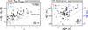 |
Fig. 6 Illustration of the two different, mutually exclusive assumptions (Sect. 6.2.3). In both figures we assume |
There are black hole mass estimates for five of our objects from broad components of the Hα emission (Nesvadba et al. 2011). They show that the black holes in powerful radio galaxies are extremely massive, MBH > 109 M⊙, but based on such a small number, a characterisation of the black hole properties over our entire sample is difficult. However, these measurement are especially useful for comparison with the assumptions in the following sections.
To increase the number of MBH estimates, we will use empirical relationships based on both Mstel and to estimate the black hole mass in our sample. These two approaches are somewhat degenerate, as they use the same data with two different sets of assumptions. We first define the assumptions made in using the total stellar mass and the local MBH–MBulge relation to estimate black hole masses. We then use the infrared luminosity of the AGN combined with this mass to calculate the Eddington ratio. We also present a second approach where we fix the Eddington ratio (λ = 0.1) and then use the infrared luminosity of the AGN to estimate the black hole mass. We took these two approaches to constrain the possible ranges for the Eddington ratios and/or black hole masses and to isolate the impact of the various assumptions that go into these sorts of estimates. We also mention the systematics that would affect our results when relevant, and summarise them in Appendix D.
6.2.1. Black hole mass
As previously noted, all the galaxies in our sample have estimated stellar masses (Seymour et al. 2007; De Breuck et al. 2010). All are very massive, with Mstel> 1011M⊙. When HST imaging is available, the best-fit light profiles are consistent with n = 4 profile (Pentericci et al. 2001, Appendix D), suggesting that the luminosity weighted mass distribution has a spheroidal morphology (even if some discrepancies are observed). Since the mass of the black hole is related to the spheroidal mass11, we can use the local MBH–MBulge relationship to estimate the black hole mass, MBH(Häring & Rix 2004),  (3)where MBH and Mbulge are in M⊙. We therefore refer to this approximation as the local approximation (see Fig. 6, left).
Out of the five sources in our sample with independent black hole mass estimates, only one MBH is directly comparable given the upper limits on the stellar mass (due to AGN torus contribution in the other four sources in the near-IR). For this source, MRC 0156-252, the derived MBH from stellar mass lies at a factor ~4 below that estimated using the broad Hα emission. The four remaining sources also suggest a significant offset with respect to the MBH–MBulge relation (see Fig. 4 in Nesvadba et al. 2011). We will therefore refer to this offset as the N11 offset.
6.2.2. Eddington ratio
The Eddington ratio represents the rate at which a black hole is accreting compared to the maximal accretion rate considering a spherical accretion (i.e. Eddington limit). This Eddington ratio (λ) is defined as 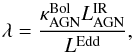 (4)where is in L⊙, is the bolometric correction from IR (set to 6 here; see Sect. 6.1.2, Appendices C, and D) and the Eddington luminosity (the maximal luminosity radiated at given black hole mass), LEdd, is defined as
  (5)where mp is the mass of the proton, G the gravitational constant, c the speed of light, σT the Thomson cross section of the electron, LEdd is in L⊙ and
  in M⊙. Rearranging Eqs. (4) and (5), one can obtain an estimate of the black hole mass for a given Eddington ratio and IR luminosity. Observations on quasars show a typical Eddington ratio λ ~ 0.1 (Kollmeier et al. 2006; Vestergaard & Osmer 2009; Ballo et al. 2012). We therefore consider an alternate black hole mass defined through Eqs. (4) and (5), making use of and setting λ = 0.1. We refer to this approximation as the 10% Eddington approximation (see Fig. 6, right; Appendix C; and Appendix D for a discussion of the systematic effects).
6.2.3. Two hypotheses on Eddington ratio and black hole mass
Figure 6 summarises the two previously introduced methods to estimate MBH (with stellar mass, Sect. 6.2.1 the local approximation and Eddington ratio, Sect. 6.2.2, the 10% Eddington approximation).
The left panel presents the Eddington ratios calculated assuming the local MBH–MBulge relation with black diamonds and with the N11 offset from the same relation from Nesvadba et al. (2011) as empty squares. The latter implies a lower λ because they have a larger black hole mass. We also illustrate the Eddington limit (λ = 1). While λ suggests an increasing trend with redshift (factor of ~10 between z = 1 and z = 3, with or without the N11 offset), the main difference holds in the range of Eddington ratios. We stress that our uncertainties on MBH are still consistent with black holes close to the Eddington limit in both approximations without any need to invoke super Eddington accretion. Anyway, this is interesting as it suggests that to grow rapidly, the SMBH need to accrete close to the Eddington limit to produce their high bolometric luminosities. Moreover, this result seems consistent with quasars, where an increase in λ between z = 2 and z = 6 has been observed (e.g. Willott et al. 2010; Urrutia et al. 2012).
The right panel presents the two different inferred black hole masses (local and 10% Eddington) plotted against each other. It is clear from this plot that in the case of the 10% Eddington approximation, all black holes appear more massive than suggested by the local MBH–MBulge relation, i.e. above the dashed line (1:1 relation). As a comparison, we overplot the black hole mass measurements for Nesvadba et al. (2011) scaled from the right axis (in blue). It seems that the 10% Eddington approximation reproduces the measured black hole masses from Nesvadba et al. (2011) (within a factor of 2).
Independently from these assumptions, we observe here MBH > 109 M⊙ at z> 1. Optical studies of SDSS quasars (e.g. Vestergaard & Osmer 2009) show that, although rare, MBH > 109 M⊙ are not exceptional at high-redshift. This implies that such extremely massive black holes have acquired most of their mass by z = 2–4 as no significantly more massive black holes are found in the local Universe (Kormendy & Ho 2013, for a recent review). We would therefore be observing the progenitors of the most massive and quiescent black holes at z = 0.
We warn that the last results are degenerate. The only way to overcome this deficiency is through independent measurements of the black hole masses or better constraints on the Eddington ratio (λ). Constraining the former allows us to bypass the MBH–MBulge relation, while constraining the latter allows us to estimate the black hole mass without the 10% Eddington approximation (λ = 0.1).
6.3. Specific growth properties
Two of the most challenging questions in modern astrophysics are determining the relative growth rate of galaxies and how this growth is related to the growth and activity of their central supermassive black holes. The relative growth of galaxies and their black holes can be specified as the specific star formation rate (sSFR) and the specific black hole accretion rate (sṀBH). Galaxies at high and low redshift follow a reasonably tight “main sequence” of star formation in the SFR-M⋆ plane (e.g. Noeske et al. 2007; Elbaz et al. 2007, 2011). How is the relative growth rate of the stellar mass of radio galaxies related to the general population of star forming galaxies? We have already shown that powerful high-redshift radio galaxies form stars at very high rates, but they are also massive. Are their relative growth rates, their sSFR, higher than normal star forming galaxies? Being very luminous AGN, we know their black hole accretion rates are high, but is the supermassive black hole growing at a relative rate that is consistent with maintaining the relationship of spheroid mass and black hole mass similar to what is observed at low redshift?
6.3.1. sSFR of high-redshift radio galaxies
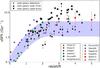 |
Fig. 7 The specific star formation rate (sSFR, in Gyr-1) as a function of redshift. The various coloured points represent measurements from the literature at M⋆ ~ 1010M⊙; see the references in the legend at the bottom right. Since the slope of the sSFR-M⋆ relation is approximately zero, the rate at which the sSFR evolves is largely independent of M⋆. Thus, this is an appropriate comparison, even for galaxies as massive as the radio galaxies studied here. The black stars, triangles, and upside-down triangles represent the radio galaxy detections, lower limits, and upper limits to the sSFR, respectively. The blue shaded region represents the scatter in the observed sSFR values (±0.3 dex). This rendition of the evolution of the sSFR was inspired by a similar plot in Weinmann et al. (2011). See also Lenhert et al. (in prep.). |
The specific star formation rate provides an estimate of the instantaneous relative stellar mass growth rates of galaxies. If galaxies are able to sustain their star formation over a significant time and at the rate observed, the inverse of the sSFR is the mass doubling time scale. Interestingly, the mass doubling time scale is shorter than a Hubble time at all redshifts, becoming comparable to the Hubble time at z = 0. This suggests that if the galaxies have long duty cycles, they can grow relatively quickly at high-redshift. Over the redshift range spanned by our radio galaxy sample, the sSFR of the population of star forming galaxies is approximately constant (~2 Gyr-1) or slowly increases with redshift (e.g. Feulner et al. 2005; Rodighiero et al. 2010; Stark et al. 2013; Ilbert et al. 2013).
Compared to the ensemble of distant star forming galaxies, we find that generally the radio galaxies are growing more rapidly (Fig. 7). The combination of upper limits in the Herschel photometry and the stellar masses, the number of galaxies with constrained sSFR is only a fraction of the entire sample (~30%). Nevertheless, a significant trend for the sSFRs of the radio galaxies to increase with increasing redshift can be seen. This increase can be characterised in the following way: at z ≲ 2.5, the sSFR of the radio galaxies is comparable to that of the normal star forming galaxy population (i.e. no AGN), whereas at z ≳ 2.5, the radio galaxies lie significantly above (about a factor of 3) the galaxy population. The scatter for the radio galaxies is a bit higher than in the galaxy population, ~±0.5 dex compared to ~±0.3 dex for the non-AGN galaxies. However, given the more limited number of radio galaxies, this difference is not significant. The offset to higher values by a factor of ~3 for the radio galaxies at z ≳ 2.5 is significant. This offset is to be compared to the systematic uncertainties associated with the calculation of the sSFR (see Appendix D). Notably, the uncertainties on the IMF are already taken into account in the blue area (Weinmann et al. 2011). Overall, the results might shift because of systematic uncertainties, but differentially, it is unlikely to wipe out any differences between our sample and the ensemble of galaxies. We also note that radio galaxies are at the bright end of the K-z diagram (Rocca-Volmerange et al. 2004), and present comparable to SMGs (see Sect. 6.1.1), so they are naturally expected to lie in a different area of the SFR-M∗ diagram than normal, more quiescent galaxies (e.g. Elbaz et al. 2011).
The cause of the offset at higher redshifts in the sSFR of radio galaxies compared to the normal population of star forming galaxies is not known. Morphological evidence for galaxies lying above the main sequence of star formation suggests that mergers may play a significant role in increasing the sSFR (e.g. De Breuck et al. 2005; Elbaz et al. 2011; Sargent et al. 2013). This picture seems consistent with the trend for radio galaxies to appear in disturbed systems (e.g. Ivison et al. 2008, 2012; Seymour et al. 2012; Wylezalek et al. 2013b). However, whether or not merging is the only cause of perturbed systems is still an open question for the sample of radio galaxies studied here, especially in light of the fact that radio galaxies generally lie in galaxy overdensities (Pascarelle et al. 1996; Venemans et al. 2007; Overzier et al. 2008; Kuiper et al. 2010; Wylezalek et al. 2013a). Galaxies in overdensities at high-redshift may preferentially have higher sSFRs (Elbaz et al. 2007; Cooke et al., in prep.).
Whatever the cause of their elevated sSFRs, what is clear is that the mass doubling time of the powerful radio galaxy population is short, only about 100 Myr at z ≳ 2.5. If such a relative growth rate could be sustained for 1 Gyr, the typical radio galaxy would grow by a factor of 1000. Thus, despite their high masses, the current star formation rate and relative growth rate do not need to be sustained for a significant fraction of the local Hubble time (1–2 Gyrs over the redshift range spanned in our sample). Notably, the mass depletion time scales are generally very short, of the order of 100 Myr or less (Ivison et al. 2012; Emonts et al. 2011, 2013). This either suggests that powerful radio galaxies generally represent the last phases of their rapid growth or that, given their relatively rich environments, they are being continuously (re-)fuelled. Their large stellar masses, significantly greater than the fiducial stellar mass turnover in the galaxy co-moving volume density and their overall consistency with the old ages derived for local early-type galaxies, suggest these are the almost fully formed progenitors of local early-type galaxies (Bernardi et al. 2010). So it may well be that these galaxies are at the end of their formation epoch. They likely formed the bulk of their stars at much higher redshifts, consistent with the stellar synthesis fitting to the broadband SEDs of a few of these galaxies (Rocca-Volmerange et al. 2013).
6.3.2. Specific black hole accretion rate
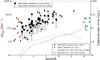 |
Fig. 8 sṀBH versus redshift. sṀBH is reported here with the two assumptions on black hole masses discussed on Fig. 6. The black filled squares are the local MBH–MGal assumption and the empty square the offset expected from (Nesvadba et al. 2011,see Sect. 6.2.3). We also report other QSO samples for comparison (as indicated in the legend; Willott et al. 2010; Urrutia et al. 2012). In addition, we compare our specific accretion rates with predictions of two models for the growth rate of MBH = 109 M⊙ black holes similar to our mass estimates (dashed and solid thick lines, see text for details; Shankar et al. 2013). |
The specific black hole accretion rate (sṀBH) corresponds to the inverse of the mass doubling time for the black hole. Following Shankar et al. (2013), sṀBH can be defined as  (6)where λ is the Eddington ratio (calculated in Sect. 6.2.2), and f is the actual fraction of mass feeding the black hole and increasing its mass, defined as f = ϵ/ (1 − ϵ), where ϵ is the radiative efficiency factor (see Eq. (2)). Figure 8 presents a mildly increasing value of sṀBH with redshift, a flattening at z = 4–5, and then a possible decline at z> 6. This behaviour is very similar to what we observed in the sSFR (Fig. 8). The characteristic time for the growth of the black hole is tS< 100 Myr for λ> 0.5 and ϵ = 0.1 (see Sect. 6.2.2 and Appendix D for related uncertainties).
How do these estimates compare to other classes of powerful AGN? In order to compare our radio galaxies to similar objects, we also show estimates of sṀBH from various samples of quasars from the literature and we use Eq. (6) to calculate sṀBH from the Eddington ratio for these samples. The high-redshift sample from Willott et al. (2010) provides the necessary constraints for high-redshift optically selected quasars at z ~ 6.2, while the sample from Urrutia et al. (2012) provides this information for the lower redshift (z ~ 0.7) red quasars. Both of these samples of quasars have similar specific accretion rates compared to high redshift radio galaxies under a similar set of assumptions. And so we can conclude that high specific accretion rates appear to be a generic feature of bolometrically luminous AGN, whether or not they are radio loud.
In addition, Fig. 8 also compares our specific accretion rate estimates with models for the growth of supermassive black holes (Shankar et al. 2013). The models we are specifically comparing to are for the evolution of very massive black holes, MBH = 109 M⊙, similar to what we think are the best mass estimates for the black holes in these radio galaxies (Nesvadba et al. 2011). The models of Shankar et al. (2013) that satisfy the most observational constraints are those that allow the peak of an assumed Gaussian distribution of Eddington accretion rates to evolve with redshift, G(z), or with both redshift and black hole mass, G(z, MBH). These models for MBH = 109 M⊙ fall far below our estimates, by 1–2 orders of magnitude. While these models seek to reproduce the average growth rate of very massive black holes, they fail to reproduce the intense growing phase known as the quasar mode. However, black holes this massive are rare and do not contribute significantly to the overall growth of black holes at high-redshift. However, it is also true that because of their extreme masses lying at the exponential end of the mass function, they provide strong constraints on any model. This is especially true given their potential impact on their host galaxies. Having specific accretion rates off by orders of magnitude means the impact of the AGN on its surroundings, whether it be the surrounding interstellar, intra-cluster, or intergalactic medium, will be greatly underestimated.
6.4. Are the SMBHs outgrowing their hosts?
The accretion rate of the BH compared to the SFR (Fig. 3), the relatively high BH accretion rates relative to the Eddington limit (Fig. 6), and sṀBH compared to sSFR (Fig. 9) all seem to suggest that the supermassive black holes in powerful radio galaxies at high-redshift may have out-grown and/or may be outgrowing their host galaxies. Whether the black hole is too massive compared to its host, or it is accreting at large Eddington ratio, the black hole of radio galaxies is or will be (in the near future) off the MBH–MBulge relation. This offset happens when the black holes grow very rapidly, with characteristic times of <100 Myr for doubling their masses. At the same time the stellar mass of the hosts also grow very rapidly, but apparently not rapidly enough (Fig. 9). Thus, to recover the local ratio of black hole and host mass as observed locally, the host of radio galaxies needs to catch up with their overly massive black holes. We therefore have potential evidence for non-coeval growth of the radio galaxies and their central black holes. In the process, black holes appear to grow extremely quickly and efficiently at first, then the host catches up, only to fall again to the observed local ratio MBH/Mgal.
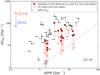 |
Fig. 9 The specific star formation rate (sSFR, in Gyr-1) versus the specific black hole accretion rate, sṀBH (in Gyr-1). The galaxies with constrained estimates of both sSFR and sṀBH are shown in red, while the arrows indicated upper or lower limits for each or both quantities. sṀBH was estimated using the local MBH–MBulge relation (filled red diamonds) or using the N11 offset (empty red squares, see Sect. 6.2.3). The dashed line indicates where the sṀBH = sSFR. |
Knowing the duration of the AGN phase would allow us to estimate the time lag, Rlag, which is how long the host galaxy will need to grow at its current rate to get back on the local ratio of stellar to black hole mass. We can calculate this relative time lag assuming a simple model of constant growth or at least a growth rate with a well-defined average. We define the final mass of the galaxy (or BH) after a episode of growth as a linear equation, 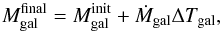 (7)where ΔTgal is the duration of the star formation (or fueling of the black hole, ΔTBH), Ṁgal is the star formation rate (or the mass accretion rate onto the black hole, ṀBH), and the initial,
  , and final mass of the galaxy,
  (or BH,
  and
and  ). We parameterise the growth of galaxies and black holes in exactly the same linear way. Assuming that the galaxy and the black hole start and end on the ratio of their masses as defined by the local stellar mass of the spheroid mass black hole mass relationship, dividing the two equations allows us to estimate the ratio of the duration of the star formation and the mass accretion onto the BH that enables the galaxies to have the local Mgal/MBH ratio. Dividing these two equations and rearranging the terms gives
 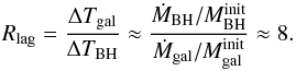 (8)The relative time for the mass of the galaxy to catch up with mass of the black hole such that it falls back onto the local MBH–MBulge relation, Rlag is simply the ratio between the sṀBH and sSFR. For our simple model, this means if the black hole growth lasts for 20 Myr, the typical lifetime of a quasar phase (e.g. Steidel et al. 2002; Hopkins et al. 2005), the galaxy will need at least 160 Myr to catch up with the black hole growth. This is assuming that the actual measured growth rate is the average over the time over which the growth occurred under our given framework (see Sects. 6.1.1–6.3.2). This simplistic model shows that galaxy activity needs to be much longer than the AGN phase in order to catch up after the relative rapid black hole growth. This would naturally explain the observation that the black holes in radio galaxies lie preferentially above the MBH–Mgal relation. It may be that the mass of the BH already lies above the relation (Nesvadba et al. 2011), which would then require even more time for the host galaxy to catch up.
6.5. The future evolution of powerful radio galaxies
We have found that the stellar populations and supermassive black holes of radio galaxies grow very rapidly. They can double their respective masses in a few 100 Myr or less. Interestingly, it appears that, relatively, the supermassive black hole is outgrowing or has outgrown its host galaxy. Crudely speaking, the host galaxy will require about an order of magnitude longer than the lifetime of the AGN for the host galaxy to catch up. “Catching up” in this context means how much longer will it take for the galaxy at its current sSFR to have a mass sufficient to land on the local MBH–MBulge relation once the BH growth has slowed. We propose here to explore different scenarios making use of our previously calculated parameters:
High-redshift powerful radio galaxies will never land on the MBH – MBulge relation.
In the case of an over-massive black hole (compared to its host), Rlag indicates that the black hole and its host do not grow at the same rate. The gas supply on larger scales can satisfy the necessary condition to feed simultaneously both the black hole and its host galaxy over the same timescale (although we note the severe problems in terms of the physical processes required to bring the gas down to the central engine; Alexander & Hickox 2012). However, joint feeding implies that radio galaxies might never land on the local MBH–MBulge relation. In the local Universe only a handful of deviant objects have been observed (e.g. van den Bosch et al. 2012). This scenario is plausible since powerful high-redshift radio galaxies are rare objects (only few hundred have been observed out to z = 5 so far).
High-redshift powerful radio galaxies will eventually land on the MBH – MBulge relation.
A variation of the previous scenario can be proposed. The galaxies can experience their growth through mergers. Several merging scenarios can be instigated, both major/minor and gas-poor/gas-rich mergers. Major mergers are rare events, but they are expected to be mostly gas rich at high-redshift as the gas fraction increases significantly (e.g. Tacconi et al. 2010). Notably, in the case of a major merger, gas can be efficiently brought to the inner part of the galaxy (<1 kpc) and probably feeds the black hole and star formation simultaneously, allowing a new episode of black hole growth. The triggering event of the radio galaxy episode is still an open discussion, but recent studies suggest that major mergers can play an important role (e.g. Ramos Almeida et al. 2013). In the case of minor mergers, gas-rich companions could form the stars and be accreted within the cosmic time. This scenario is supported by some observational evidence thanks to high-resolution imaging with HST (Miley et al. 2006; Seymour et al. 2012). This is also related to the size evolution of galaxies as well as the compactness of early-type galaxies at high-redshift (e.g. Daddi et al. 2005; van Dokkum et al. 2008; Delaye et al. 2014), the change in the mass function with cosmic time (Ilbert et al. 2013), the light profiles and elemental abundance ratios in the outer regions of massive ellipticals (Huang et al. 2013; Greene et al. 2013), and the fact that at constant co-moving density, the mass of massive early-type galaxies grew by about a factor of 4 over approximately the last 10 Gyr (e.g. van Dokkum et al. 2010; Ilbert et al. 2013). As HzRGs are found in dense environments, probably in the centre of proto-clusters (e.g. Wylezalek et al. 2013a), they are likely to experience an important series of minor dry mergers, consistent with the size evolution scenario. Therefore, high-redshift powerful radio galaxies will finally land on the MBH–MBulge at z = 0.
High-redshift powerful radio galaxies will land on the MBH – MBulge relation, but on a longer timescale.
In the case of black holes starting on the local relation and experiencing a fast, important growth, they will be significantly off the MBH–MBulge relation in a relatively short timescale (~ 10 Myr). The host, at the current sSFR, will need roughly ten times longer in order to catch up with the black hole. Nevertheless, several observations suggest the contrary. To support such a high SFR, an important, continuous supply of gas is required. Such large amounts of gas is presently available in the HzRG systems (e.g. Emonts et al. 2013). Nevertheless, this gas possesses properties which indicate that even if a host growth is possible, it is unlikely to happen in this short timescale. High-redshift powerful radio galaxies present copious outflows of ionised and neutral gas (Nesvadba et al. 2006, 2007), gas with substantial angular momentum (van Ojik et al. 1996; Humphrey et al. 2008), or gas in the close environment (Ivison et al. 2012; Emonts et al. 2013). Before participating in the host growth, this gas needs first to be driven into the galaxy. Our best guess is that this gas will actually participate in the host growth, but in a later episode of star formation. The Rlag is therefore a lower limit of the time lag between the black hole and its host.
High-redshift powerful radio galaxies are examples of symbiotic growth.
A variation of the previous scenario is obtained by invoking a shorter timescale for the important black hole growth (<1 Myr) so the host at the current star formation can keep up with its black hole much more easily. A typical starburst can last for tens of Myrs (e.g. Kennicutt 1998). Although convenient, this scenario implies that we are looking at the very peak of the AGN activity for all sources and not at the peak of their star formation. If possible, this is unlikely to be the case, given the large scatter seen, for instance, in Fig. 3 and because the radio selection of our sources is uncorrelated with the IR luminosity (Sect. 5.3). Moreover, as mentioned earlier, the variability does induce scatter in our distributions, but does not play a fundamental role on average.
More observations at high-resolution throughout the electromagnetic spectrum, and especially tighter constraints on the BH mass and the mass of the spheroidal component of radio galaxies are needed to test these different scenarios (see Sects. 6.1.1–6.3.2 for our adopted assumptions and Appendix D for a summary of the uncertainties)
7. Conclusion
We present new Herschel and submm observations for the HeRGÉ sample consisting of 70 powerful radio galaxies spanning 1 <z< 5.2. Complemented by other data sets, we now have continuous coverage of the IR spectral energy distribution over the range of 16–870 μm. All galaxies in our sample have integrated IR luminosities LIR> 1012 L⊙, classifying them as ULIRGs, while half of all the sources at z> 2 have LIR> 1013L⊙ and are HyLIRGs.
We use the DecompIR code to decompose the IR SEDs of galaxies in our sample in a robust and uniform way into AGN and SB components. To make these fits, we assume a single AGN template and a variety of starburst templates. Our results for the AGN contribution are conservative in that we assumed a single template and it is possible that this template could lead to an underestimate of its contribution to the IR SED. The estimated and from our decomposition imply both high black hole mass accretion rates (1 M⊙ yr-1 < ṀBH < 100 M⊙ yr-1) and vigorous on-going star formation (100 M⊙ yr-1 < SFR < 5000 M⊙ yr-1). Although no strong correlation is detected between these rates, this result implies that both the black hole and its host galaxy are experiencing rapid growth, with the relative growth of the black hole exceeding that of the host galaxy.
Assuming empirical relations and basic physical assumptions, we estimate MBH from the stellar masses and infrared AGN luminosities. The black holes appear overly massive compared to their hosts and are likely accreting close to the Eddington limit (λ ~ 1), similar to estimates for radio quiet quasars. Alternatively, for lower Eddington rates, the black holes are more massive than predicted by the local MBH–MBulge relationship.
We derive the specific growth properties, both the specific star formation rate, sSFR, and the specific black hole mass accretion rate, sṀBH. Compared to galaxies that lie along the sSFR-stellar mass relation at z ≳ 2.5, radio galaxies appear to have higher sSFR. At z ≲ 2.5, radio galaxies generally appear to have the same or perhaps lower sSFR.
We explore different scenarios for the future growth of radio galaxies. These scenarios are that high-redshift powerful radio galaxies (i) will never land on the MBH–MBulge relation; (ii) will land on the local MBH–MBulge relation, but at low redshift; (iii) will land on the MBH–MBulge on a longer timescale than our estimated Rlag; or (iv) are experiencing symbiotic growth. However, observational evidence favours the scenario in which radio galaxies will land again on the MBH–MBulge relation, but on a long timescale (most probably ≫100 Myr).
Online material
Herschel observations. All are part of the OT1 seymour 1 program except when specified.
Herschel photometry.
Submm flux at 870 μm with LABOCA in this paper and at 850 μm for all the rest.
Main results from the SED fitting.
Appendix A: Notes on sources
B2 0902+34 (WCD with three detections): this object is the only radio galaxy from our sample to be most likely dominated by synchrotron emission (Archibald et al. 2001). We therefore treat this galaxy as if it were actually a member of the UL class for the purposes of fitting its SED.
4C 23.56 (WD with five detections): this object is the prototypical case where the IR emission is dominated by the emission from the AGN. There are other pieces of evidence from other wavelengths to support this dominance. For instance, rest frame UV shows strong polarisation (Cimatti et al. 1998); the IRAC colours are characteristic of sources dominated by AGN emission in rest frame near-IR (Fig. 13 De Breuck et al. 2010); X-ray emission is also prominent and suggestive of emission from an AGN. This radio source can be seen as having the most extreme AGN contribution to its SED in our sample. We stress that the Mullaney AGN template satisfactorily reproduces the SED of 4C 23.56 without any modification. This indicates that the AGN DecompIR template can be a good representation of AGN emission in our sample.
4C 41.17 (WCD with seven detections): of course, with a radio galaxy dominated by its AGN in the infrared, it would be interesting to have the opposite, a radio galaxy dominated with its IR SED dominated by star formation; 4C 41.17 very likely represents such a case. This radio source has a SB dominated SED, and can be reproduced well by the SB6 template. A more complete SED decomposition confirms this results (Rocca-Volmerange et al. 2013).
Appendix B: AGN or SB dominated?
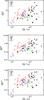 |
Fig. B.1 From top to bottom, AGN fraction at 10, 50 and 100 μm against the total infrared luminosity. The colour and symbols correspond to the classes defined in Sect. 3.2. |
We note that fAGN is defined as the ratio SAGN/SSB where S is the flux of the AGN and the SB respectively, at 10, 50, and 100 μm. Figure B.1 plots the  fraction as a function of the total infrared luminosity, (see Sect. 3.1). This fraction of AGN emission at 10, 50, and 100 μm allow us to check whether the emission at the probed wavelength is dominated by AGN emission or not.
The top plot shows that, independently from the classification introduced in Sect. 3.2, the AGN contributes at least 50% of the flux at 10 μm. In contrast, at 100 μm (bottom plot), the AGN is generally at the ≲10% level. However, we can see that even at such long wavelengths, the contribution of the AGN can, from time to time, be exceptionally high (almost 50%). This last value could refer to extreme objects such as 4C 23.56 or to extended dust emission (Dicken et al. 2010). At 50 μm (middle plot), we can clearly see that AGN can be from dominant to completely negligible. We conclude that even trying to define classes to potentially differentiate between AGN and SB dominated objects from data is almost impossible for high-redshift radio galaxies. Only a SED decomposition as presented in Sect. 4 can finally settle this question.
Appendix C: Bolometric correction
In order to derive AGN intrinsic properties, the AGN bolometric luminosity is needed. Hard X-rays provide the best approximation to the bolometric luminosity as most of the material along the line of sight is optically transparent. We do not possess X-ray measurements for our entire sample and so we make use of the calculated infrared luminosities. Numerous attempts to derive bolometric correction factors have been done (e.g. Elvis et al. 1994; Haas et al. 2003; Marconi et al. 2004; Krawczyk et al. 2013; Hao et al. 2014; Scott & Stewart 2014). Although essential, they are subject to significative variation from object to object. For our SED range, Elvis et al. (1994) and Richards et al. (2006) provide some correction factors depending on the observed wavelength. This correction factor can be as small as 2 and as high as 20 for X-rays, depending mainly on the morphology. Here, we want an approximation of this factor for our sources.
First, we can use a purely geometrical approach. Assuming the torus around AGN to be optically thick at all wavelengths, it absorbs light from across the electromagnetic spectrum and re-radiates in IR. We can use the statistical distribution of Type 1 and Type 2 AGN in the sky (Barthel 1989). The solid angle for an opening angle of 45°corresponds to a factor ~2. This is expected to be the minimum correction.
Second, we can assume that the nuclei in Type 2 and Type 1 AGN are similar. Using a Type 1 radio loud AGN template from Elvis et al. (1994) and assuming that the total IR luminosity does not depend strongly on orientation, the bolometric correction factor is ~6. Doing the same exercise with the Richards et al. (2006) template gives a correction factor of ~5.
Third, some sources in our sample possess X-ray observations (Carilli et al. 2002). Integrating the energy over X-rays, it appears that X-rays do not present the most significative contribution to the bolometric luminosity.
As the radio emission is highly directional (i.e. subject to strong beaming effects), its inclusion in the bolometric factor is highly uncertain. Type 2 AGN SEDs show that the integrated radio energy is roughly at the X-ray level. Its contribution to the total energy should not be the most significant.
Estimation of the bolometric correction is rather difficult and uncertain. Nevertheless, the geometric approach and the moderate contribution from X-rays and radio indicates that most of the light comes from the UV-optical from the central AGN part and the reprocessed light from the dust. Therefore, a factor of 6 seems appropriate in the case of radio galaxies to convert to .
Appendix D: Summary of the global uncertainties
Since we are using various approximations throughout this paper that can have an impact on this analysis, we summarise here each of these and discuss their possible impact on our interpretation.
-
(i)
The validity of the MBH–MBulge relation at high-redshift de-serves some attention. The first part of this relation is to considerthe estimated stellar mass as the mass of the bulge or spheroid ofindividual galaxies. HST observations have shown that radiogalaxies have elliptical light profiles (van Breugelet al. 1998; Pentericciet al. 1999, 2001; Zirmet al. 2003). Nevertheless, thesedeterminations represent the radially averaged or globalbest-fit light profile with moderate-to-low signal-to-noiseand the possible presence and contribution from substruc-ture and heavily obscured younger disc components cannotbe excluded in the profile fitting (see Hatchet al. 2013). After all, our estimatesof the star formation rates suggest that obscuration could be im-portant and since the gas supporting such intense star formationwould be highly dissipative and could easily be in a disc. However,the stellar masses estimated by De Breuck et al. (2010) are measured in the rest-frame H band, minimizing the impact of extinction and also sampling more appropriately the older population (modulo the contribution from young super-giants). The measured mass can therefore be considered as the total mass of the system and at least, in principle, sensitive to the older generations of stars in the host galaxy (Rocca-Volmerange et al. 2013). Considering the MBH–MBulge relation itself, Jahnke et al. (2009) estimate that the MBH-Mstel relation shows little variation from z = 1.4 to z = 0.
-
(ii)
The radiative efficiency of the accretion, ϵ, is not well-constrained and is certainly not a constant. This factor can vary from 0.06 to 0.42, related to the spin of the black hole (Krolik 1999). There are attempts to constrain the spin of radio loud AGN in the literature. Martínez-Sansigre & Rawlings (2011) show that black hole spins tend to be lower at higher redshift even with the presence of a bimodal distribution. As these constraints are quite poor at high-redshift, it is impossible to draw a conclusion on the possible value of ϵ, but perhaps a range of a few is reasonable (a factor of 3 at most).
-
(iii)
The correction factor to estimate the bolometric luminosity,
, shows a wide variety of possible values. Pure geometric considerations imply that  and is unlikely to be >10 for the conversion of IR luminosity to bolometric luminosity (see Appendix C for details). We assumed for the ensemble of radio galaxies. This correction is not expected to differ strongly from this value as the energy is mostly radiated in IR in our object and we have now good coverage of this part of the SED. However, a factor as low as 2 is not unreasonable (see Appendix C).
 -
(iv)
The calculated sSFR are dependant on the canonical law used to transform
into SFR and the stellar mass. While the Kennicutt (1998) relation seems to represent most star forming galaxies, some discrepancies are expected as it is dependent of the star formation law. Calzetti (2012) lists the impact of the approximation on the different SFR indicators at various wavelengths. This also depends on τ and the adopted IMF; the variation can be a factor of a few (up to ~6). In addition, the IMF can induce a factor of ~2 in the stellar masses estimates (e.g. Marchesini et al. 2009). This effect will move the points horizontally in Fig. 9. -
(v)
The AGN SED can present a wide variation (e.g. Nenkova et al. 2008; Fritz et al. 2006). As mentioned, our generic AGN SED can miss a part of the extended flux from the AGN heating of the NLR (e.g. Dicken et al. 2009; Pier & Krolik 1993). However, as we are dealing with integrated luminosities over the 8–1000 μm range, the calculated
is expected to differ strongly only with a drastic change of the AGN SED which is unlikely (Sect. 4.2). The most probable case would be that we underestimated the AGN contribution; therefore, all corresponding values will be increased by the same factor, increasing the offset from the local MBH–MBulge relation.
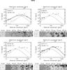 |
Fig. D.1 SEDs of the 70 radiogalaxies sorted by RA. IRS and MIPS data taken from De Breuck et al. (2010), PACS and SPIRE data in Table 3, and submm data in Table 4. Filled diamonds are the firm detections (>3σ), open diamonds the weak detections (2σ<Fgal< 3σ), and downward triangles the 3σ upper limits. The red downward triangles mark to the most constraining upper limit. Continuous line represents for fitted components, depending on the class: AGN for WD, SB for CD, and sum of AGN and SB for WCD (as marked in the figure legend). The six stamps correspond to the MIPS (24 μm) and the five Herschel observations when available, with north at the top, east at the left, centred on the radio coordinates of the radio galaxy. Each stamp covers 2 × 2 arcmin. We also overplot the IRS spectra when available for the source (Seymour et al. 2008; Rawlings et al. 2013). |
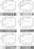 |
Fig. D.1 continued. |
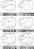 |
Fig. D.1 continued. |
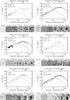 |
Fig. D.1 continued. |
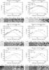 |
Fig. D.1 continued. |
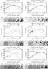 |
Fig. D.1 continued. |
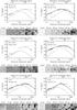 |
Fig. D.1 continued. |
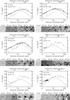 |
Fig. D.1 continued. |
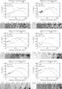 |
Fig. D.1 continued. |
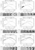 |
Fig. D.1 continued. |
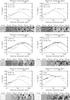 |
Fig. D.1 continued. |
 |
Fig. D.1 continued. |
We also test the reduction with smaller pixel size (1.2 and 2.1 arcsec for the blue/green and red channels) and find the differences on the final flux to be negligible (<5%). See also PICC-ME-TN-033 (April 4, 2012 v2) at http://herschel.esac.esa.int/twiki/pub/Public/PacsCalibrationWeb/bolopsf_20.pdf for further information on the pixelisation effect on the PSF.
Due to k-correction effects, a part of the IRS filter falls outside the template for z> 2.5. We therefore extrapolate the templates to λ = 2 μm using a power-law function. This modification does not affect our results as the energy contribution from these wavelengths (2 μm <λ< 3 μm) is negligible compared to the total IR luminosity.
Classified as a WD, this extreme object appears to be the prototype of the pure AGN contribution (see Appendix A and Fig. D.1).
At 500 MHz, the radio emission is dominated by the lobes. At this frequency, relativistic beaming effects do not play a significant role (Blundell et al. 1998).
The and SFR from our SED decomposition are also compatible with the previous estimates based on the IRS spectra Seymour et al. (2008) and Rawlings et al. (2013).
Even in the case of a non-spheroidal geometry, the most important factor appears to be the observed mass of the galaxy, with little evolution with redshift (Jahnke et al. 2009, Appendix D).
Acknowledgments
G.D. warmly thanks Clive Tadhunter and Rob Ivison for their comments allowing a significative improvement of this paper. G.D. also thanks the referee for his comments that helped to clarify this paper. N.S. is the recipient of an Australian Research Council Future Fellowship. F.E.B. acknowledges support from Basal-CATA PFB-06/2007 and CONICYT-Chile grants FONDECYT 1101024 and Anillo ACT1101. E.I. acknowledges funding from CONICYT/FONDECYT postdoctoral project N°: 3130504. The work of D.S. was carried out at Jet Propulsion Laboratory, California Institute of Technology, under a contract with NASA. Herschel is an ESA space observatory with science instruments provided by European-led Principal Investigator consortia and with important participation from NASA. This work is based in part on observations made with the Spitzer Space Telescope. This work is based on observations made with the APEX Telescope, based on the Chajnantor Plateau in Chile. HIPE is a joint development by the Herschel Science Ground Segment Consortium, consisting of ESA, the NASA Herschel Science Center, and the HIFI, PACS, and SPIRE consortia. Facilities: Spitzer, Herschel, APEX
References
- Aird, J., Nandra, K., Laird, E. S., et al. 2010, MNRAS, 401, 2531 [NASA ADS] [CrossRef] [Google Scholar]
- Alexander, D. M., & Hickox, R. C. 2012, New A Rev., 56, 93 [NASA ADS] [CrossRef] [Google Scholar]
- Alexander, D. M., Smail, I., Bauer, F. E., et al. 2005, Nature, 434, 738 [NASA ADS] [CrossRef] [PubMed] [Google Scholar]
- Antonucci, R. 2012, Astron. Astrophys. Trans., 27, 557 [NASA ADS] [Google Scholar]
- Archibald, E. N., Dunlop, J. S., Hughes, D. H., et al. 2001, MNRAS, 323, 417 [NASA ADS] [CrossRef] [Google Scholar]
- Asmus, D., Gandhi, P., Smette, A., Hönig, S. F., & Duschl, W. J. 2011, A&A, 536, A36 [NASA ADS] [CrossRef] [EDP Sciences] [Google Scholar]
- Ballo, L., Heras, F. J. H., Barcons, X., & Carrera, F. J. 2012, A&A, 545, A66 [NASA ADS] [CrossRef] [EDP Sciences] [Google Scholar]
- Barger, A. J., Cowie, L. L., Sanders, D. B., et al. 1998, Nature, 394, 248 [NASA ADS] [CrossRef] [Google Scholar]
- Barthel, P. D. 1989, ApJ, 336, 606 [Google Scholar]
- Barthel, P., Haas, M., Leipski, C., & Wilkes, B. 2012, ApJ, 757, L26 [NASA ADS] [CrossRef] [Google Scholar]
- Bernardi, M., Shankar, F., Hyde, J. B., et al. 2010, MNRAS, 404, 2087 [NASA ADS] [Google Scholar]
- Blain, A. W., Smail, I., Ivison, R. J., & Kneib, J.-P. 1999, MNRAS, 302, 632 [NASA ADS] [CrossRef] [Google Scholar]
- Blundell, K. M., Rawlings, S., Eales, S. A., Taylor, G. B., & Bradley, A. D. 1998, MNRAS, 295, 265 [NASA ADS] [CrossRef] [Google Scholar]
- Blundell, K. M., Rawlings, S., & Willott, C. J. 1999, AJ, 117, 677 [Google Scholar]
- Bongiorno, A., Merloni, A., Brusa, M., et al. 2012, MNRAS, 427, 3103 [NASA ADS] [CrossRef] [Google Scholar]
- Bornancini, C. G., O’Mill, A. L., Gurovich, S., & Lambas, D. G. 2010, MNRAS, 406, 197 [NASA ADS] [CrossRef] [Google Scholar]
- Calzetti, D. 2012, Proc. XXII Canary Island Winter School of Astrophysics: Secular Evolution of Galaxies, eds. J. Falcon-Barroso, & J. H. Knapen [Google Scholar]
- Cao, X., & Li, F. 2008, MNRAS, 390, 561 [NASA ADS] [CrossRef] [Google Scholar]
- Carilli, C. L., Roettgering, H. J. A., van Ojik, R., Miley, G. K., & van Breugel, W. J. M. 1997, ApJS, 109, 1 [NASA ADS] [CrossRef] [Google Scholar]
- Carilli, C. L., Harris, D. E., Pentericci, L., et al. 2002, ApJ, 567, 781 [NASA ADS] [CrossRef] [Google Scholar]
- Chapman, S. C., Blain, A. W., Smail, I., & Ivison, R. J. 2005, ApJ, 622, 772 [NASA ADS] [CrossRef] [Google Scholar]
- Chen, C.-T. J., Hickox, R. C., Alberts, S., et al. 2013, ApJ, 773, 3 [NASA ADS] [CrossRef] [Google Scholar]
- Cimatti, A., di Serego Alighieri, S., Vernet, J., Cohen, M., & Fosbury, R. A. E. 1998, ApJ, 499, L21 [NASA ADS] [CrossRef] [Google Scholar]
- Cleary, K., Lawrence, C. R., Marshall, J. A., Hao, L., & Meier, D. 2007, ApJ, 660, 117 [NASA ADS] [CrossRef] [Google Scholar]
- Crocker, A. F., Bureau, M., Young, L. M., & Combes, F. 2011, MNRAS, 410, 1197 [NASA ADS] [CrossRef] [Google Scholar]
- Daddi, E., Renzini, A., Pirzkal, N., et al. 2005, ApJ, 626, 680 [NASA ADS] [CrossRef] [Google Scholar]
- Daddi, E., Dickinson, M., Morrison, G., et al. 2007, ApJ, 670, 156 [NASA ADS] [CrossRef] [Google Scholar]
- Dale, D. A., Helou, G., Magdis, G. E., et al. 2014, ApJ, 784, 83 [NASA ADS] [CrossRef] [Google Scholar]
- Davis, S. W., & Laor, A. 2011, ApJ, 728, 98 [CrossRef] [Google Scholar]
- De Breuck, C., van Breugel, W., Stanford, S. A., et al. 2002, AJ, 123, 637 [NASA ADS] [CrossRef] [Google Scholar]
- De Breuck, C., Downes, D., Neri, R., et al. 2005, A&A, 430, L1 [NASA ADS] [CrossRef] [EDP Sciences] [Google Scholar]
- De Breuck, C., Seymour, N., Stern, D., et al. 2010, ApJ, 725, 36 [NASA ADS] [CrossRef] [Google Scholar]
- Del Moro, A., Alexander, D. M., Mullaney, J. R., et al. 2013, A&A, 549, A59 [NASA ADS] [CrossRef] [EDP Sciences] [Google Scholar]
- Delaye, L., Huertas-Company, M., Mei, S., et al. 2014, MNRAS, 441, 203 [NASA ADS] [CrossRef] [Google Scholar]
- Dey, A., van Breugel, W., Vacca, W. D., & Antonucci, R. 1997, ApJ, 490, 698 [NASA ADS] [CrossRef] [Google Scholar]
- Dicken, D., Tadhunter, C., Axon, D., et al. 2009, ApJ, 694, 268 [NASA ADS] [CrossRef] [Google Scholar]
- Dicken, D., Tadhunter, C., Axon, D., et al. 2010, ApJ, 722, 1333 [NASA ADS] [CrossRef] [Google Scholar]
- Dicken, D., Tadhunter, C., Axon, D., et al. 2012, ApJ, 745, 172 [NASA ADS] [CrossRef] [Google Scholar]
- Diolaiti, E., Bendinelli, O., Bonaccini, D., et al. 2000, A&AS, 147, 335 [NASA ADS] [CrossRef] [EDP Sciences] [Google Scholar]
- Draine, B. T. 2003, ARA&A, 41, 241 [NASA ADS] [CrossRef] [Google Scholar]
- Drouart, G., De Breuck, C., Vernet, J., et al. 2012, A&A, 548, A45 [NASA ADS] [CrossRef] [EDP Sciences] [Google Scholar]
- Elbaz, D., Daddi, E., Le Borgne, D., et al. 2007, A&A, 468, 33 [NASA ADS] [CrossRef] [EDP Sciences] [Google Scholar]
- Elbaz, D., Dickinson, M., Hwang, H. S., et al. 2011, A&A, 533, A119 [NASA ADS] [CrossRef] [EDP Sciences] [Google Scholar]
- Elvis, M., Wilkes, B. J., McDowell, J. C., et al. 1994, ApJS, 95, 1 [NASA ADS] [CrossRef] [Google Scholar]
- Emonts, B. H. C., Feain, I., Mao, M. Y., et al. 2011, ApJ, 734, L25 [NASA ADS] [CrossRef] [Google Scholar]
- Emonts, B. H. C., Feain, I., Röttgering, H. J. A., et al. 2013, MNRAS, 430, 3465 [NASA ADS] [CrossRef] [Google Scholar]
- Engel, H., Tacconi, L. J., Davies, R. I., et al. 2010, ApJ, 724, 233 [NASA ADS] [CrossRef] [Google Scholar]
- Esquej, P., Alonso-Herrero, A., González-Martín, O., et al. 2014, ApJ, 780, 86 [Google Scholar]
- Falder, J. T., Stevens, J. A., Jarvis, M. J., et al. 2010, MNRAS, 405, 347 [NASA ADS] [Google Scholar]
- Feltre, A., Hatziminaoglou, E., Hernán-Caballero, A., et al. 2013, MNRAS, 434, 2426 [NASA ADS] [CrossRef] [Google Scholar]
- Ferrarese, L., & Merritt, D. 2000, ApJ, 539, L9 [NASA ADS] [CrossRef] [Google Scholar]
- Feulner, G., Gabasch, A., Salvato, M., et al. 2005, ApJ, 633, L9 [NASA ADS] [CrossRef] [Google Scholar]
- Fioc, M., & Rocca-Volmerange, B. 1997, A&A, 326, 950 [NASA ADS] [Google Scholar]
- Fitzpatrick, E. L. 1999, PASP, 111, 63 [NASA ADS] [CrossRef] [Google Scholar]
- Fritz, J., Franceschini, A., & Hatziminaoglou, E. 2006, MNRAS, 366, 767 [Google Scholar]
- Galametz, A., Stern, D., De Breuck, C., et al. 2012, ApJ, 749, 169 [NASA ADS] [CrossRef] [Google Scholar]
- Gebhardt, K., Bender, R., Bower, G., et al. 2000, ApJ, 539, L13 [NASA ADS] [CrossRef] [Google Scholar]
- Greene, J. E., Murphy, J. D., Graves, G. J., et al. 2013, ApJ, 776, 64 [NASA ADS] [CrossRef] [Google Scholar]
- Griffin, M. J., Abergel, A., Abreu, A., et al. 2010, A&A, 518, L3 [Google Scholar]
- Haas, M., Klaas, U., Müller, S. A. H., et al. 2003, A&A, 402, 87 [NASA ADS] [CrossRef] [EDP Sciences] [Google Scholar]
- Hainline, L. J., Blain, A. W., Smail, I., et al. 2011, ApJ, 740, 96 [NASA ADS] [CrossRef] [Google Scholar]
- Hao, C.-N., Xia, X.-Y., Shu-DeMao, Deng, Z.-G., & Wu, H. 2008, Chin. J. Astron. Astrophys., 8, 12 [Google Scholar]
- Hao, H., Elvis, M., Civano, F., et al. 2014, MNRAS, 438, 1288 [NASA ADS] [CrossRef] [Google Scholar]
- Hardcastle, M. J., & Worrall, D. M. 1999, MNRAS, 309, 969 [NASA ADS] [CrossRef] [Google Scholar]
- Hardcastle, M. J., Evans, D. A., & Croston, J. H. 2007, MNRAS, 376, 1849 [NASA ADS] [CrossRef] [Google Scholar]
- Häring, N., & Rix, H.-W. 2004, ApJ, 604, L89 [NASA ADS] [CrossRef] [Google Scholar]
- Harrison, C. M., Alexander, D. M., Mullaney, J. R., et al. 2012, ApJ, 760, L15 [NASA ADS] [CrossRef] [Google Scholar]
- Hatch, N. A., Overzier, R. A., Röttgering, H. J. A., Kurk, J. D., & Miley, G. K. 2008, MNRAS, 383, 931 [NASA ADS] [CrossRef] [Google Scholar]
- Hatch, N. A., De Breuck, C., Galametz, A., et al. 2011, MNRAS, 410, 1537 [NASA ADS] [Google Scholar]
- Hatch, N. A., Röttgering, H. J. A., Miley, G. K., et al. 2013, MNRAS, 436, 2244 [NASA ADS] [CrossRef] [Google Scholar]
- Hatziminaoglou, E., Omont, A., Stevens, J. A., et al. 2010, A&A, 518, L33 [NASA ADS] [CrossRef] [EDP Sciences] [Google Scholar]
- Hickox, R. C., Myers, A. D., Brodwin, M., et al. 2011, ApJ, 731, 117 [NASA ADS] [CrossRef] [Google Scholar]
- Hickox, R. C., Mullaney, J. R., Alexander, D. M., et al. 2014, ApJ, 782, 9 [NASA ADS] [CrossRef] [Google Scholar]
- Hicks, E. K. S., Davies, R. I., Malkan, M. A., et al. 2009, ApJ, 696, 448 [NASA ADS] [CrossRef] [Google Scholar]
- Hodge, J. A., Karim, A., Smail, I., et al. 2013, ApJ, 768, 91 [NASA ADS] [CrossRef] [Google Scholar]
- Hopkins, A. M., & Beacom, J. F. 2006, ApJ, 651, 142 [NASA ADS] [CrossRef] [MathSciNet] [Google Scholar]
- Hopkins, P. F., & Quataert, E. 2010, MNRAS, 407, 1529 [NASA ADS] [CrossRef] [Google Scholar]
- Hopkins, P. F., Hernquist, L., Martini, P., et al. 2005, ApJ, 625, L71 [Google Scholar]
- Hopkins, P. F., Hernquist, L., Cox, T. J., et al. 2006, ApJS, 163, 1 [Google Scholar]
- Huang, S., Ho, L. C., Peng, C. Y., Li, Z.-Y., & Barth, A. J. 2013, ApJ, 768, L28 [NASA ADS] [CrossRef] [Google Scholar]
- Hughes, D. H., Serjeant, S., Dunlop, J., et al. 1998, Nature, 394, 241 [NASA ADS] [CrossRef] [Google Scholar]
- Humphrey, A., Villar-Martín, M., Vernet, J., et al. 2008, MNRAS, 383, 11 [NASA ADS] [CrossRef] [Google Scholar]
- Ilbert, O., McCracken, H. J., Le Fèvre, O., et al. 2013, A&A, 556, A55 [NASA ADS] [CrossRef] [EDP Sciences] [Google Scholar]
- Ivison, R. J., Morrison, G. E., Biggs, A. D., et al. 2008, MNRAS, 390, 1117 [NASA ADS] [CrossRef] [Google Scholar]
- Ivison, R. J., Smail, I., Amblard, A., et al. 2012, MNRAS, 425, 1320 [NASA ADS] [CrossRef] [Google Scholar]
- Jahnke, K., Bongiorno, A., Brusa, M., et al. 2009, ApJ, 706, L215 [NASA ADS] [CrossRef] [Google Scholar]
- Janssen, R. M. J., Röttgering, H. J. A., Best, P. N., & Brinchmann, J. 2012, A&A, 541, A62 [NASA ADS] [CrossRef] [EDP Sciences] [Google Scholar]
- Jogee, S., Scoville, N., & Kenney, J. D. P. 2005, ApJ, 630, 837 [NASA ADS] [CrossRef] [Google Scholar]
- Kaiser, C. R., Dennett-Thorpe, J., & Alexander, P. 1997, MNRAS, 292, 723 [NASA ADS] [CrossRef] [Google Scholar]
- Karim, A., Swinbank, A. M., Hodge, J. A., et al. 2013, MNRAS, 432, 2 [NASA ADS] [CrossRef] [Google Scholar]
- Kartaltepe, J. S., Sanders, D. B., Le Floc’h, E., et al. 2010, ApJ, 709, 572 [NASA ADS] [CrossRef] [Google Scholar]
- Kennicutt, Jr., R. C. 1998, ARA&A, 36, 189 [Google Scholar]
- Ker, L. M., Best, P. N., Rigby, E. E., Röttgering, H. J. A., & Gendre, M. A. 2012, MNRAS, 420, 2644 [NASA ADS] [CrossRef] [Google Scholar]
- Klamer, I. J., Ekers, R. D., Bryant, J. J., et al. 2006, MNRAS, 371, 852 [NASA ADS] [CrossRef] [Google Scholar]
- Kollmeier, J. A., Onken, C. A., Kochanek, C. S., et al. 2006, ApJ, 648, 128 [NASA ADS] [CrossRef] [Google Scholar]
- Kormendy, J., & Ho, L. C. 2013, ARA&A, 51, 511 [Google Scholar]
- Kovács, A. 2008, in SPIE Conf. Ser., 7020, 45 [Google Scholar]
- Krawczyk, C. M., Richards, G. T., Mehta, S. S., et al. 2013, ApJS, 206, 4 [NASA ADS] [CrossRef] [Google Scholar]
- Krolik, J. H. 1999, Active galactic nuclei: from the central black hole to the galactic environment [Google Scholar]
- Kuiper, E., Hatch, N. A., Röttgering, H. J. A., et al. 2010, MNRAS, 405, 969 [NASA ADS] [Google Scholar]
- Kuiper, E., Hatch, N. A., Venemans, B. P., et al. 2011, MNRAS, 417, 1088 [NASA ADS] [CrossRef] [Google Scholar]
- Labbé, I., Huang, J., Franx, M., et al. 2005, ApJ, 624, L81 [NASA ADS] [CrossRef] [Google Scholar]
- Lauer, T. R., Faber, S. M., Richstone, D., et al. 2007, ApJ, 662, 808 [NASA ADS] [CrossRef] [Google Scholar]
- Lehnert, M. D., & Heckman, T. M. 1996, ApJ, 472, 546 [NASA ADS] [CrossRef] [Google Scholar]
- Leipski, C., Haas, M., Willner, S. P., et al. 2010, ApJ, 717, 766 [NASA ADS] [CrossRef] [Google Scholar]
- Leipski, C., Meisenheimer, K., Walter, F., et al. 2013, ApJ, 772, 103 [NASA ADS] [CrossRef] [Google Scholar]
- Leipski, C., Meisenheimer, K., Walter, F., et al. 2014, ApJ, 785, 154 [NASA ADS] [CrossRef] [Google Scholar]
- Magdis, G. E., Elbaz, D., Dickinson, M., et al. 2011, A&A, 534, A15 [NASA ADS] [CrossRef] [EDP Sciences] [Google Scholar]
- Magorrian, J., Tremaine, S., Richstone, D., et al. 1998, AJ, 115, 2285 [NASA ADS] [CrossRef] [Google Scholar]
- Marchesini, D., van Dokkum, P. G., Förster Schreiber, N. M., et al. 2009, ApJ, 701, 1765 [NASA ADS] [CrossRef] [Google Scholar]
- Marconi, A., Risaliti, G., Gilli, R., et al. 2004, MNRAS, 351, 169 [NASA ADS] [CrossRef] [Google Scholar]
- Martínez-Sansigre, A., & Rawlings, S. 2011, MNRAS, 414, 1937 [NASA ADS] [CrossRef] [Google Scholar]
- Matthews, T. A., Morgan, W. W., & Schmidt, M. 1964, ApJ, 140, 35 [NASA ADS] [CrossRef] [Google Scholar]
- Merloni, A., Rudnick, G., & Di Matteo, T. 2004, MNRAS, 354, L37 [NASA ADS] [CrossRef] [Google Scholar]
- Merloni, A., Bongiorno, A., Bolzonella, M., et al. 2010, ApJ, 708, 137 [NASA ADS] [CrossRef] [Google Scholar]
- Michalowski, M. J., Dunlop, J. S., Cirasuolo, M., et al. 2012, A&A, 541, A85 [NASA ADS] [CrossRef] [EDP Sciences] [Google Scholar]
- Miley, G., & De Breuck, C. 2008, A&ARv, 15, 67 [NASA ADS] [CrossRef] [Google Scholar]
- Miley, G. K., Overzier, R. A., Zirm, A. W., et al. 2006, ApJ, 650, L29 [NASA ADS] [CrossRef] [Google Scholar]
- Mullaney, J. R., Alexander, D. M., Goulding, A. D., & Hickox, R. C. 2011, MNRAS, 414, 1082 [NASA ADS] [CrossRef] [Google Scholar]
- Nenkova, M., Sirocky, M. M., Ivezić, Ž., & Elitzur, M. 2008, ApJ, 685, 147 [NASA ADS] [CrossRef] [Google Scholar]
- Nesvadba, N. P. H., Lehnert, M. D., Eisenhauer, F., et al. 2006, ApJ, 650, 693 [NASA ADS] [CrossRef] [Google Scholar]
- Nesvadba, N. P. H., Lehnert, M. D., De Breuck, C., Gilbert, A., & van Breugel, W. 2007, A&A, 475, 145 [NASA ADS] [CrossRef] [EDP Sciences] [Google Scholar]
- Nesvadba, N. P. H., Lehnert, M. D., De Breuck, C., Gilbert, A. M., & van Breugel, W. 2008, A&A, 491, 407 [NASA ADS] [CrossRef] [EDP Sciences] [Google Scholar]
- Nesvadba, N. P. H., De Breuck, C., Lehnert, M. D., et al. 2011, A&A, 525, A43 [NASA ADS] [CrossRef] [EDP Sciences] [Google Scholar]
- Netzer, H. 2009, MNRAS, 399, 1907 [NASA ADS] [CrossRef] [Google Scholar]
- Nguyen, H. T., Schulz, B., Levenson, L., et al. 2010, A&A, 518, L5 [NASA ADS] [CrossRef] [EDP Sciences] [Google Scholar]
- Noeske, K. G., Weiner, B. J., Faber, S. M., et al. 2007, ApJ, 660, L43 [Google Scholar]
- Ogle, P., Whysong, D., & Antonucci, R. 2006, ApJ, 647, 161 [NASA ADS] [CrossRef] [Google Scholar]
- Ott, S. 2010, in Astronomical Data Analysis Software and Systems XIX, eds. Y. Mizumoto, K.-I. Morita, & M. Ohishi, ASP Conf. Ser., 434, 139 [Google Scholar]
- Overzier, R. A., Bouwens, R. J., Cross, N. J. G., et al. 2008, ApJ, 673, 143 [NASA ADS] [CrossRef] [Google Scholar]
- Pascarelle, S. M., Windhorst, R. A., Driver, S. P., Ostrander, E. J., & Keel, W. C. 1996, ApJ, 456, L21 [NASA ADS] [CrossRef] [Google Scholar]
- Pearson, C., Lim, T., North, C., et al. 2013, Exp. Astron. [arXiv:1401.2036] [Google Scholar]
- Pentericci, L., Röttgering, H. J. A., Miley, G. K., et al. 1999, A&A, 341, 329 [NASA ADS] [Google Scholar]
- Pentericci, L., Van Reeven, W., Carilli, C. L., Röttgering, H. J. A., & Miley, G. K. 2000, A&AS, 145, 121 [NASA ADS] [CrossRef] [EDP Sciences] [Google Scholar]
- Pentericci, L., McCarthy, P. J., Röttgering, H. J. A., et al. 2001, ApJS, 135, 63 [NASA ADS] [CrossRef] [Google Scholar]
- Pier, E. A., & Krolik, J. H. 1993, ApJ, 418, 673 [NASA ADS] [CrossRef] [Google Scholar]
- Pilbratt, G. L., Riedinger, J. R., Passvogel, T., et al. 2010, A&A, 518, L1 [CrossRef] [EDP Sciences] [Google Scholar]
- Poglitsch, A., Waelkens, C., Geis, N., et al. 2010, A&A, 518, L2 [NASA ADS] [CrossRef] [EDP Sciences] [Google Scholar]
- Popesso, P., Magnelli, B., Buttiglione, S., et al. 2012, A&A, submitted [arXiv:1211.4257] [Google Scholar]
- RamosAlmeida, C., Bessiere, P. S., Tadhunter, C. N., et al. 2013, MNRAS, 436, 997 [NASA ADS] [CrossRef] [Google Scholar]
- Rawlings, J. I., Seymour, N., Page, M. J., et al. 2013, MNRAS, 429, 744 [NASA ADS] [CrossRef] [Google Scholar]
- Reuland, M., van Breugel, W., Röttgering, H., et al. 2003, ApJ, 592, 755 [NASA ADS] [CrossRef] [Google Scholar]
- Reuland, M., Röttgering, H., van Breugel, W., & De Breuck, C. 2004, MNRAS, 353, 377 [NASA ADS] [CrossRef] [Google Scholar]
- Richards, G. T., Lacy, M., Storrie-Lombardi, L. J., et al. 2006, ApJS, 166, 470 [NASA ADS] [CrossRef] [Google Scholar]
- Rocca-Volmerange, B., Le Borgne, D., De Breuck, C., Fioc, M., & Moy, E. 2004, A&A, 415, 931 [NASA ADS] [CrossRef] [EDP Sciences] [Google Scholar]
- Rocca-Volmerange, B., Drouart, G., De Breuck, C., et al. 2013, MNRAS, 429, 2780 [NASA ADS] [CrossRef] [Google Scholar]
- Rodighiero, G., Vaccari, M., Franceschini, A., et al. 2010, A&A, 515, A8 [NASA ADS] [CrossRef] [EDP Sciences] [Google Scholar]
- Rosario, D. J., Santini, P., Lutz, D., et al. 2012, A&A, 545, A45 [NASA ADS] [CrossRef] [EDP Sciences] [Google Scholar]
- Rosario, D. J., Burtscher, L., Davies, R., et al. 2013, ApJ, 778, 94 [NASA ADS] [CrossRef] [Google Scholar]
- Roseboom, I. G., Oliver, S. J., Kunz, M., et al. 2010, MNRAS, 409, 48 [NASA ADS] [CrossRef] [Google Scholar]
- Sargent, M. T., Daddi, E., Béthermin, M., et al. 2013, ApJ, submitted [arXiv:1303.4392] [Google Scholar]
- Schuller, F. 2012, in SPIE Conf. Ser., 8452 [Google Scholar]
- Scott, A. E., & Stewart, G. C. 2014, MNRAS, 438, 2253 [NASA ADS] [CrossRef] [Google Scholar]
- Seymour, N., Stern, D., De Breuck, C., et al. 2007, ApJS, 171, 353 [NASA ADS] [CrossRef] [Google Scholar]
- Seymour, N., Ogle, P., De Breuck, C., et al. 2008, ApJ, 681, L1 [NASA ADS] [CrossRef] [Google Scholar]
- Seymour, N., Altieri, B., De Breuck, C., et al. 2012, ApJ, 755, 146 [NASA ADS] [CrossRef] [Google Scholar]
- Shankar, F., Weinberg, D. H., & Shen, Y. 2010, MNRAS, 406, 1959 [NASA ADS] [Google Scholar]
- Shankar, F., Weinberg, D. H., & Miralda-Escudé, J. 2013, MNRAS, 428, 421 [NASA ADS] [CrossRef] [Google Scholar]
- Shen, Y., Strauss, M. A., Oguri, M., et al. 2007, AJ, 133, 2222 [NASA ADS] [CrossRef] [Google Scholar]
- Simpson, J., Swinbank, M., Smail, I., et al. 2013, ApJ, accepted [arXiv:1310.6363] [Google Scholar]
- Somerville, R. S., Primack, J. R., & Faber, S. M. 2001, MNRAS, 320, 504 [NASA ADS] [CrossRef] [Google Scholar]
- Stark, D. P., Schenker, M. A., Ellis, R., et al. 2013, ApJ, 763, 129 [NASA ADS] [CrossRef] [Google Scholar]
- Steidel, C. C., Hunt, M. P., Shapley, A. E., et al. 2002, ApJ, 576, 653 [NASA ADS] [CrossRef] [Google Scholar]
- Stevens, J. A., Ivison, R. J., Dunlop, J. S., et al. 2003, Nature, 425, 264 [NASA ADS] [CrossRef] [PubMed] [Google Scholar]
- Swinbank, A. M., Simpson, J. M., Smail, I., et al. 2014, MNRAS, 438, 1267 [Google Scholar]
- Symeonidis, M., Vaccari, M., Berta, S., et al. 2013, MNRAS, 431, 2317 [NASA ADS] [CrossRef] [Google Scholar]
- Tacconi, L. J., Genzel, R., Smail, I., et al. 2008, ApJ, 680, 246 [NASA ADS] [CrossRef] [PubMed] [Google Scholar]
- Tacconi, L. J., Genzel, R., Neri, R., et al. 2010, Nature, 463, 781 [Google Scholar]
- Thomas, D., Maraston, C., Bender, R., & Mendes de Oliveira, C. 2005, ApJ, 621, 673 [NASA ADS] [CrossRef] [Google Scholar]
- Urrutia, T., Lacy, M., Spoon, H., et al. 2012, ApJ, 757, 125 [NASA ADS] [CrossRef] [Google Scholar]
- van Breugel, W. J. M., Stanford, S. A., Spinrad, H., Stern, D., & Graham, J. R. 1998, ApJ, 502, 614 [NASA ADS] [CrossRef] [Google Scholar]
- van den Bosch, R. C. E., Gebhardt, K., Gültekin, K., et al. 2012, Nature, 491, 729 [NASA ADS] [CrossRef] [PubMed] [Google Scholar]
- van Dokkum, P. G., Franx, M., Kriek, M., et al. 2008, ApJ, 677, L5 [NASA ADS] [CrossRef] [Google Scholar]
- van Dokkum, P. G., Whitaker, K. E., Brammer, G., et al. 2010, ApJ, 709, 1018 [NASA ADS] [CrossRef] [Google Scholar]
- van Ojik, R., Roettgering, H. J. A., Carilli, C. L., et al. 1996, A&A, 313, 25 [NASA ADS] [Google Scholar]
- Venemans, B. P., Röttgering, H. J. A., Miley, G. K., et al. 2007, A&A, 461, 823 [NASA ADS] [CrossRef] [EDP Sciences] [Google Scholar]
- Vernet, J., Fosbury, R. A. E., Villar-Martín, M., et al. 2001, A&A, 366, 7 [NASA ADS] [CrossRef] [EDP Sciences] [Google Scholar]
- Vestergaard, M., & Osmer, P. S. 2009, ApJ, 699, 800 [Google Scholar]
- Videla, L., Lira, P., Andrews, H., et al. 2013, ApJS, 204, 23 [NASA ADS] [CrossRef] [Google Scholar]
- Volonteri, M., Sikora, M., & Lasota, J.-P. 2007, ApJ, 667, 704 [NASA ADS] [CrossRef] [Google Scholar]
- Wang, R., Wagg, J., Carilli, C. L., et al. 2011, AJ, 142, 101 [NASA ADS] [CrossRef] [Google Scholar]
- Wang, S. X., Brandt, W. N., Luo, B., et al. 2013, ApJ, 778, 179 [NASA ADS] [CrossRef] [Google Scholar]
- Wardlow, J. L., Smail, I., Coppin, K. E. K., et al. 2011, MNRAS, 415, 1479 [NASA ADS] [CrossRef] [Google Scholar]
- Weinmann, S. M., Neistein, E., & Dekel, A. 2011, MNRAS, 417, 2737 [NASA ADS] [CrossRef] [Google Scholar]
- Weiß, A., Kovács, A., Coppin, K., et al. 2009, ApJ, 707, 1201 [NASA ADS] [CrossRef] [Google Scholar]
- Willott, C. J., Albert, L., Arzoumanian, D., et al. 2010, AJ, 140, 546 [NASA ADS] [CrossRef] [Google Scholar]
- Willott, C. J., Omont, A., & Bergeron, J. 2013, ApJ, 770, 13 [NASA ADS] [CrossRef] [Google Scholar]
- Wylezalek, D., Galametz, A., Stern, D., et al. 2013a, ApJ, 769, 79 [NASA ADS] [CrossRef] [Google Scholar]
- Wylezalek, D., Vernet, J., De Breuck, C., et al. 2013b, MNRAS, 428, 3206 [NASA ADS] [CrossRef] [Google Scholar]
- Young, L. M., Bureau, M., Davis, T. A., et al. 2011, MNRAS, 414, 940 [NASA ADS] [CrossRef] [Google Scholar]
- Zhang, X., Lu, Y., & Yu, Q. 2012, ApJ, 761, 5 [NASA ADS] [CrossRef] [Google Scholar]
- Zirm, A. W., Dickinson, M., & Dey, A. 2003, ApJ, 585, 90 [NASA ADS] [CrossRef] [Google Scholar]
All Tables
Distribution of the sample as a function of their class and their number of detections in the IR.
Herschel observations. All are part of the OT1 seymour 1 program except when specified.
All Figures
|
Fig. 1 Total IR luminosity ( |
| In the text | |
|
Fig. 2 Left: |
| In the text | |
|
Fig. 3
|
| In the text | |
|
Fig. 4
|
| In the text | |
|
Fig. 5
|
| In the text | |
|
Fig. 6 Illustration of the two different, mutually exclusive assumptions (Sect. 6.2.3). In both figures we assume |
| In the text | |
|
Fig. 7 The specific star formation rate (sSFR, in Gyr-1) as a function of redshift. The various coloured points represent measurements from the literature at M⋆ ~ 1010M⊙; see the references in the legend at the bottom right. Since the slope of the sSFR-M⋆ relation is approximately zero, the rate at which the sSFR evolves is largely independent of M⋆. Thus, this is an appropriate comparison, even for galaxies as massive as the radio galaxies studied here. The black stars, triangles, and upside-down triangles represent the radio galaxy detections, lower limits, and upper limits to the sSFR, respectively. The blue shaded region represents the scatter in the observed sSFR values (±0.3 dex). This rendition of the evolution of the sSFR was inspired by a similar plot in Weinmann et al. (2011). See also Lenhert et al. (in prep.). |
| In the text | |
|
Fig. 8 sṀBH versus redshift. sṀBH is reported here with the two assumptions on black hole masses discussed on Fig. 6. The black filled squares are the local MBH–MGal assumption and the empty square the offset expected from (Nesvadba et al. 2011,see Sect. 6.2.3). We also report other QSO samples for comparison (as indicated in the legend; Willott et al. 2010; Urrutia et al. 2012). In addition, we compare our specific accretion rates with predictions of two models for the growth rate of MBH = 109 M⊙ black holes similar to our mass estimates (dashed and solid thick lines, see text for details; Shankar et al. 2013). |
| In the text | |
|
Fig. 9 The specific star formation rate (sSFR, in Gyr-1) versus the specific black hole accretion rate, sṀBH (in Gyr-1). The galaxies with constrained estimates of both sSFR and sṀBH are shown in red, while the arrows indicated upper or lower limits for each or both quantities. sṀBH was estimated using the local MBH–MBulge relation (filled red diamonds) or using the N11 offset (empty red squares, see Sect. 6.2.3). The dashed line indicates where the sṀBH = sSFR. |
| In the text | |
|
Fig. B.1 From top to bottom, AGN fraction at 10, 50 and 100 μm against the total infrared luminosity. The colour and symbols correspond to the classes defined in Sect. 3.2. |
| In the text | |
|
Fig. D.1 SEDs of the 70 radiogalaxies sorted by RA. IRS and MIPS data taken from De Breuck et al. (2010), PACS and SPIRE data in Table 3, and submm data in Table 4. Filled diamonds are the firm detections (>3σ), open diamonds the weak detections (2σ<Fgal< 3σ), and downward triangles the 3σ upper limits. The red downward triangles mark to the most constraining upper limit. Continuous line represents for fitted components, depending on the class: AGN for WD, SB for CD, and sum of AGN and SB for WCD (as marked in the figure legend). The six stamps correspond to the MIPS (24 μm) and the five Herschel observations when available, with north at the top, east at the left, centred on the radio coordinates of the radio galaxy. Each stamp covers 2 × 2 arcmin. We also overplot the IRS spectra when available for the source (Seymour et al. 2008; Rawlings et al. 2013). |
| In the text | |
|
Fig. D.1 continued. |
| In the text | |
|
Fig. D.1 continued. |
| In the text | |
|
Fig. D.1 continued. |
| In the text | |
|
Fig. D.1 continued. |
| In the text | |
|
Fig. D.1 continued. |
| In the text | |
|
Fig. D.1 continued. |
| In the text | |
|
Fig. D.1 continued. |
| In the text | |
|
Fig. D.1 continued. |
| In the text | |
|
Fig. D.1 continued. |
| In the text | |
|
Fig. D.1 continued. |
| In the text | |
|
Fig. D.1 continued. |
| In the text | |
Current usage metrics show cumulative count of Article Views (full-text article views including HTML views, PDF and ePub downloads, according to the available data) and Abstracts Views on Vision4Press platform.
Data correspond to usage on the plateform after 2015. The current usage metrics is available 48-96 hours after online publication and is updated daily on week days.
Initial download of the metrics may take a while.