| Issue |
A&A
Volume 694, February 2025
ZTF SN Ia DR2
|
|
|---|---|---|
| Article Number | A8 | |
| Number of page(s) | 12 | |
| Section | Cosmology (including clusters of galaxies) | |
| DOI | https://doi.org/10.1051/0004-6361/202450389 | |
| Published online | 14 February 2025 | |
ZTF SN Ia DR2: Peculiar velocities’ impact on the Hubble diagram
1
Aix Marseille Univ, CNRS/IN2P3, CPPM, Marseille, France
2
Department of Physics, Duke University, Durham, NC 27708, USA
3
Université Clermont-Auvergne, CNRS, LPCA, 63000 Clermont-Ferrand, France
4
School of Physics, Trinity College Dublin, College Green, Dublin 2, Ireland
5
Oskar Klein Centre, Department of Astronomy, Stockholm University, SE-10691 Stockholm, Sweden
6
Institut für Physik, Humboldt Universität zu Berlin, Newtonstr 15, 12101 Berlin, Germany
7
Univ. Lyon, Univ. Claude Bernard Lyon 1, CNRS, IP2I Lyon/IN2P3, UMR 5822, F-69622 Villeurbanne, France
8
Department of Physics, Lancaster University, Lancs LA1 4YB, UK
9
National Research Council of Canada, Herzberg Astronomy & Astrophysics Research Centre, 5071 West Saanich Road, Victoria, BC V9E 2E7, Canada
10
Sorbonne/Paris Cité Universités, LPNHE, CNRS/IN2P3, LPNHE, 75005 Paris, France
11
Institute of Astronomy and Kavli Institute for Cosmology, University of Cambridge, Madingley Road, Cambridge CB3 0HA, UK
12
Institute of Space Sciences (ICE, CSIC), Campus UAB, Carrer de Can Magrans, s/n, E-08193 Barcelona, Spain
13
Deutsches Elektronen Synchrotron DESY, Platanenallee 6, 15738 Zeuthen, Germany
14
Lawrence Berkeley National Laboratory, 1 Cyclotron Road MS 50B-4206, Berkeley, CA 94720, USA
15
Department of Astronomy, University of California, Berkeley, 501 Campbell Hall, Berkeley, CA 94720, USA
16
Nordic Optical Telescope, Rambla José Ana Fernández Pérez 7, ES-38711 Breña Baja, Spain
17
IPAC, California Institute of Technology, 1200 E. California Blvd, Pasadena, CA 91125, USA
18
249-17 Caltech, Pasadena, CA 91125, USA
19
Caltech Optical Observatories, California Institute of Technology, Pasadena, CA 91125, USA
20
Department of Physics, Drexel University, Philadelphia, PA 19104, USA
⋆ Corresponding authors; bastien.carreres@duke.edu, rosselli@cppm.in2p3.fr
Received:
15
April
2024
Accepted:
19
July
2024
Type Ia supernovae (SNe Ia) are used to determine the distance-redshift relation and build the Hubble diagram. Neglecting their host-galaxy peculiar velocities (PVs) may bias the measurement of cosmological parameters. The smaller the redshift, the larger the effect is. We used realistic simulations of SNe Ia observed by the Zwicky Transient Facility (ZTF) to investigate the effect of different methods of taking PVs into account. We studied the impact of neglecting galaxy PVs and their correlations in an analysis of the SNe Ia Hubble diagram. We find that it is necessary to use the PV full covariance matrix computed from the velocity power spectrum to take the sample variance into account. Considering the results we have obtained using simulations, we determine the PV systematic effects in the context of the ZTF SN Ia DR2 sample. We determine the PV impact on the intercept of the Hubble diagram, aB, which is directly linked to the measurement of H0. We show that not taking into account PVs and their correlations results in a shift in the H0 value of about 1.0 km s−1 Mpc−1 and a slight underestimation of the H0 error bar.
Key words: dark energy / distance scale / large-scale structure of Universe
© The Authors 2025
 Open Access article, published by EDP Sciences, under the terms of the Creative Commons Attribution License (https://creativecommons.org/licenses/by/4.0), which permits unrestricted use, distribution, and reproduction in any medium, provided the original work is properly cited.
This article is published in open access under the Subscribe to Open model. Subscribe to A&A to support open access publication.
1. Introduction
Type Ia supernovae (SNe Ia) are well-known standardizable candles that have been widely used to provide precise estimates of the luminosity distances to galaxies, as an input of the Hubble diagram. SNe Ia are an essential probe with which to measure cosmological parameters such as the dark matter density, the dark energy density, its equation-of-state parameter, w (Betoule et al. 2014; Brout et al. 2022), and the Hubble constant, H0 (Riess et al. 2022; Scolnic et al. 2023).
Several surveys have been designed (e.g., LSST, LSST Science Collaboration 2009; Euclid, Laureijs et al. 2011; and DESI, DESI Collaboration 2016) to collect powerful datasets for cosmology. In particular, the Zwicky Transient Facility (ZTF) was designed to observe several thousands of SN Ia light curves, by far the largest low-redshift sample (z < 0.1) to date. By combining the data from all these surveys, cosmological parameters, such as H0, w, and the matter density parameter, Ωm, will be measured with a precision never reached before, allowing us to put strong constraints on the ΛCDM model. To achieve this goal, we need to improve our understanding of different sources of systematic uncertainties that were negligible in the past compared to statistical uncertainties. In this article, we explore the effect of the SN Ia host-galaxy peculiar velocities (PVs) on the determination of H0 with the ZTF sample.
Peculiar velocities refer to the motion of galaxies with respect to a comoving frame in an expanding Universe. They originate from the gravitational infall of matter toward overdense regions. As has been demonstrated in previous works such as (Hui & Greene 2006; Davis et al. 2011; Peterson et al. 2022), the SN Ia host galaxy PVs have the most significant impact on cosmological parameter inference when using low-redshift SNe Ia. Depending on the sign of the PV projection on the observer’s line of sight, it will produce either a blue or a red Doppler shift (zp) of the observed redshift (zobs) with respect to the cosmological redshift (zcos):

The PV distribution of the host galaxies will affect the redshift-distance relation in two ways. Firstly, PVs will increase the scatter in the Hubble diagram residuals, since the observed redshifts are used to compute the predicted distance modulus, μth(zobs), for a given cosmology and μth(zobs) is directly related to the Hubble diagram residuals. We can consider that, to the first order, zp = vp/c, where vp is the galaxy PV line-of-sight component and c is the speed of light. The typical vp is on the order of several hundred km s−1. At low redshift, it corresponds to a magnitude scatter comparable to the SN Ia intrinsic scatter (see Davis et al. 2011; Carreres et al. 2023 and references therein for a detailed discussion).
Secondly, PVs are correlated spatially due to large-scale bulk motion (see Peebles 1980). The majority of previous SN Ia analyses consider PVs to be independent and randomly distributed. However, there are non-negligible correlations between galaxy velocities in different sky positions. These correlations arise because PVs are the result of galaxy motion within the same large-scale structure gravitational potential. Neglecting the PV spatial correlation when fitting the Hubble diagram may bias cosmological parameter measurements (Davis et al. 2011), especially when analyzing low-redshift SN Ia samples.
When both the distance and the redshift to a galaxy are available, one can derive an estimate of its PV. Studying the correlations of such velocities allows us to constrain the cosmic growth rate of structures, fσ8. This parameter expresses the growth of the cosmic structure throughout the history of the Universe. Various methods have been developed to perform this measurement (see Johnson et al. 2014; Howlett et al. 2017; Said et al. 2020; Turner et al. 2022; Lai et al. 2023; Carreres et al. 2023).
The Hubble constant, H0, could be measured using SNe Ia with distance anchors to calibrate the absolute magnitude, MB. The usual anchors are nearby galaxy distances measured thanks to Cepheids (Riess et al. 2022) or the tip of the red giant branch (TRGB, Dhawan et al. 2022; Scolnic et al. 2023). This allows one to obtain the absolute magnitude, MB, of the nearby SNe Ia. The SNe Ia that reside in the Hubble flow are used to determine the intercept of the Hubble diagram, aB. The intercept is linked to H0 through the relation
In recent analysis (Brout et al. 2022; Riess et al. 2022; Kenworthy et al. 2022), PVs have been corrected using PV field reconstruction methods (Lavaux & Hudson 2011; Carrick et al. 2015; Graziani et al. 2019; Lilow & Nusser 2021). The first attempts at applying these methods to correct PVs to SNe Ia in the Hubble diagram have shown improvements in the residuals (Peterson et al. 2022; Carr et al. 2022). However, these methods require a spectroscopic survey of the underlying large-scale structure. Moreover, the current literature lacks testing of these methods on simulations, which would provides a better understanding of the bias and systematics that could arise from their use in the Hubble diagram.
In this work, we study the impact of galaxy PVs and their correlations on the Hubble diagram fit in the context of the SNe Ia sample of the second ZTF Data Release from the ZTF Type Ia Supernovae and Cosmology science working group (ZTF SN Ia DR2). We make use of both realistic simulations and real data to study the systematic impact of PVs in the Hubble diagram. We determine the effect of PVs on the intercept of the Hubble diagram aB. This work will be useful for future cosmological analyses that may use the SNe Ia coming from ZTF survey.
The paper is organized as follows. In Sect. 2, we describe the data and the simulations we have used for this work. In Sect. 3, we present the method used to fit the Hubble diagram and to take into account PVs. In Sect. 4, we describe our findings when we analyze the realistic SN Ia simulations. In Sect. 5, we present our main result on the impact of PVs on the intercept of the Hubble diagram for the second data-release of the ZTF Type Ia Supernova survey. Finally, we state our conclusions in Sect. 6.
2. Data
2.1. The ZTF SN Ia DR2 sample
The ZTF (Bellm et al. 2019; Graham et al. 2019; Masci et al. 2019; Dekany et al. 2020) is an optical survey that started operating in 2018. It covers two thirds of the sky from a declination of −30° to a declination of +90°. Thanks to its 47 deg2 field of view, it observes in the g, r, and i bands with a typical magnitude depth of 20 and a cadence ranging from several visits per day to several visits per month. The detected transient sources are followed up spectroscopically for precise classification. The reduction of spectra and classification are performed by the ZTF SED machine (Blagorodnova et al. 2018; Rigault et al. 2019; Kim et al. 2022).
The SN Ia sample used in this work is the ZTF SN Ia DR2 sample (Rigault et al. 2025; Smith et al. 2025). It is a sample of SN Ia data coming from the ZTF survey between March 2018 and December 2020. It consists of 3628 SN Ia light curves, with host galaxy properties (e.g., stellar mass, g − z). All the SNe Ia have been spectroscopically classified and have spectroscopic redshifts that come from the host galaxy (∼70%), mostly given by the DESI MOST host program (Soumagnac et al. 2024), or from the SN Ia spectrum (∼30%). The host galaxy redshifts have an uncertainty of about 10−5, while the SN Ia spectrum redshifts have an uncertainty of about 10−3 (see Smith et al. 2025 for details about the SN Ia redshifts and the method of matching the SN Ia with its host galaxy). The light curves were fitted using the SALT2 model (Guy et al. 2007, 2010) and the release contains the resulting parameters: the time of the peak magnitude, t0, the stretch, x1, the color, c, and the peak magnitude in the Bessel-B band at rest frame, mB. The DR2 SNe Ia are volume-limited up to z ∼ 0.06 (Carreres et al. 2023; Amenouche et al. 2025). This constitutes the largest low-redshift SNe Ia sample to date.
In this work, we applied to the SN Ia light curves the quality cuts given in Table 1 of Rigault et al. (2025). We required at least five observations with a signal-to-noise ratio above five to ensure a good sampling of the light curves. We selected the light curves with best-fit values for stretch, |x1|< 3, and color, −0.2 < c < 0.8. We excluded the SNe Ia with too-large estimated uncertainties on those parameters by requiring that σx1 < 1, σc < 0.1 and σt0 < 1. We discarded poor fit models by requiring a p-value above 10−71. Lastly, we selected SNe Ia within the redshift range of 0.023 < zobs < 0.06. The low-redshift bound exludes SN Ia velocities correlated within our local flow, while the high-redshift bound ensures that our sample is volume-limited. After these cuts, we were left with 904 SNe Ia. We accessed the ZTF SN Ia DR2 data using the python library ztfidr2.
2.2. Simulations
To test our framework, we used simulations of ZTF SNe Ia including large-scale structure, as was performed in Carreres et al. (2023). These simulations were produced using the snsim3 python library. This software allows one to simulate a realistic SNe Ia survey on top of an N-body simulation. In this work, we used the OuterRim N-body simulation (Heitmann et al. 2019), which is a box of (3 Gpc)3 at z = 0. From this box, we created 27 sub-boxes. In order to minimize any possible correlation between them, the sub-boxes were built so that they did not overlap. For each sub-box, the observer was placed at the center and the enclosed volume was equivalent to a redshift limit of z ∼ 0.17. In Appendix A, we discuss the correlation between the different sub-boxes. We found that the correlations between the host galaxies below the redshift cut of z ∼ 0.06 in different sub-boxes are one order of magnitude below the ones between two host galaxies that are in the same mock, and thus can safely be neglected.
To be consistent, the fiducial cosmology used in our simulations matches the one used in OuterRim: a flat-ΛCDM model with parameters provided in Table 1. The number of SN Ia events to be generated was computed using the latest estimate of the rate measured from ZTF data, rP20 = 2.35 × 10⁻⁵ Mpc−3 yr−1 (Perley et al. 2020). This rate had to be rescaled to our fiducial cosmology as r = rP20(h/0.7)3 with h = H0/(100 km s−1 Mpc−1). To get more statistics for the expected number of SNe Ia per Mpc−3, we multiplied this rate by the expected 6-year duration of the full ZTF survey. Each SN Ia was randomly assigned to a halo from the N-body simulation and the halo velocity was used to compute the observed redshift. We computed the angular positions of each halo relative to the observer and kept only those lying within the ZTF angular footprint. We randomly drew the SALT2 model parameters of each SN Ia: the stretch, x1, the color, c, and the apparent peak magnitude in the Bessel-B band, mB. The stretch parameter was modeled using the redshift-dependent two-Gaussian mixture described in Nicolas et al. (2021), while the color parameter distribution follows the asymmetric model given in Scolnic & Kessler (2016, Table 1) for low z.
Cosmological parameters used in the simulation.
The apparent peak magnitude was computed starting from the Tripp formula (Tripp 1998), which gives the absolute magnitude, MB, i*, in the rest-frame Bessel-B band for SN Ia i, defined as

The α, β, and MB parameters are common to all the SNe Ia. These parameters were fixed to best-fit values from Betoule et al. (2014): α = 0.14, β = 3.1, and MB = −19.05 + 5log(h/0.7), where MB is rescaled to the fiducial cosmology. The intrinsic scatter, σM, was drawn from a normal distribution with a dispersion equal to 0.12, close to what is observed (see Betoule et al. 2014, Table 9). Finally, the apparent peak magnitude for each SN Ia was computed using
where μobs is the observed distance modulus, where the relativistic beaming due to the PV effect (Davis et al. 2011) is taken into account and is given by

μcos is the distance modulus computed for a given cosmological redshift in a given cosmological model as
where dL(z) is the luminosity distance,
and r(z) is the comoving distance.
We generated the SNe Ia with the SALT2 model input parameters to compute the true light curve for each SN Ia. We made use of the SNCOSMO package4 (Barbary et al. 2023) to model the light curves. Then we used the ZTF observation logs to obtain realistic observations from light-curve models, as is described in the following: the dates of observations and the filters used at the position of the SN Ia allow one to get a realistic sampling of the light curve, while the limiting magnitude at 5σ above the sky background, the CCD gain, and the zero point of each observation are used to get realistic fluxes and error bars. The error bars were drawn from a normal distribution, the scatter of which is given by Eq. (14) in Carreres et al. (2023).
We applied to the simulated light curves the selections described in Sect. 2.5 of Carreres et al. (2023): we discarded the light curves with fewer than two epochs with fluxes S/N > 5 and we applied the spectroscopic selection function of the ZTF Bright Transient Survey (BTS), the main survey used for the spectral classification of ZTF SNe Ia (Perley et al. 2020). After the selection, we fit the light curves using the SALT2 model to recover mb, x1, and c. We applied to the simulations the same quality cuts as for the real data (Sect. 2.1). After the quality cuts, the average number of SNe Ia across each realization is ⟨N⟩∼1672 for the 6-year span of the full ZTF survey in the redshift range 0.023 < z < 0.06. This number is lower than what could be found in the data since the ZTF SN Ia DR2 span of ∼2.8 years and has found ∼900 SNe Ia. We plot the comparison between simulations and DR2 data angular positions and redshifts distributions in Fig. 1, in which the redshift distribution has been rescaled for the difference of duration between data and the simulations. The discrepancy between the number of SNe Ia in a simulation and DR2 data could come from simulation inputs, such as a too-low value for the SNe Ia rate, but also from the fact that the simulation spectroscopic selection function is only based on the BTS one, despite a small part of the DR2 data being classified using other spectroscopic programs (see Rigault et al. 2025 for a full description).
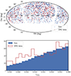 |
Fig. 1. Comparison of the angular and redshift distributions of the SNe Ia from the simulation and from the ZTF SN Ia DR2 data. Top panel: Angular positions of simulated SNe Ia from one mock (in blue) and from the DR2 data (in red). Bottom panel: Redshift distribution averaged over the 27 mocks and rescaled for the difference in the duration of the survey (in blue) compared to the DR2 redshift distribution (in red). |
The SNe Ia observed redshifts and magnitudes are affected by correlated PVs. Hence, we used the 27 realizations to test various methods to take into account PVs when fitting the Hubble diagram, as is shown in the next sections.
3. Method
We fit the Hubble diagram with a classical likelihood method that we describe in Sect. 3.1. However, we tested three ways of dealing with the PV error contribution: not accounting for PVs, including a diagonal error term, and using a full PV covariance matrix. These three approaches are described in Sect. 3.2.
3.1. Hubble diagram
Before fitting the Hubble diagram, we fit the SN Ia light curves using the SALT2 model. After the SN Ia light-curve fit, the distance modulus of each SN Ia μi was computed using the Tripp relation (Tripp 1998) as

where α, β, and M0 are free parameters of the Hubble diagram fit. The corresponding fit error bar for each SN Ia is
To fit the Hubble diagram, we maximized the likelihood given by
![$$ \begin{aligned} \mathcal{L} (\alpha , \beta , M_0) = (2\pi )^{-\frac{N}{2}} |C|^{-\frac{1}{2}}\exp \left[-\frac{1}{2}\mathbf {\Delta} \mu ^T{C}^{-1}\mathbf {\Delta} \mu \right], \end{aligned} $$](/articles/aa/full_html/2025/02/aa50389-24/aa50389-24-eq10.gif)
where C is a covariance matrix and the elements of Δμ are
with μth(z) the theoretical distance modulus (Eq. 6) computed for a given cosmology. Since ZTF is a low-redshift survey and cannot alone constrain cosmological parameters, we fixed them to a fiducial value. In our work on simulations (Sect. 4) we used the input cosmology of the simulation as the fiducial one and in our work on data (Sect. 2) we used the Planck18 results (Planck Collaboration VI 2020) as fiducial cosmology. It is worth noting that in this fit, M0 and H0 were degenerated. This necessitated that we choose a fiducial value, H0, fid, such that the M0 parameter is expressed as a combination of H0 and MB as
The fiducial value of H0 was taken to be equal to the simulation input, H0, fid = 71 km s−1 Mpc−1.
As is stated in Sect. 2.1, the ZTF SN Ia DR2 redshifts were measured with varying accuracy. We took the redshift uncertainties into account by adding the following error term to the diagonal of the covariance matrix:
where we made an approximation at the first order with respect to z.
Without taking into account the PVs, the covariance matrix is
where σM is the intrinsic scatter of the SN Ia magnitudes and is also a free parameter of the Hubble diagram fit, σSALT is given by Eq. (9), σμ − z is given by Eq. (13), and δij is the Kronecker-delta.
3.2. Peculiar velocity contribution to the error budget
As was pointed out in previous cosmological analyses, in addition to the intrinsic scatter, σM, and standardization, σSALT, error term, PVs contribute to the error budget (Cooray & Caldwell 2006; Davis et al. 2011). The total covariance for a pair of SNe Ia is then
where zi and zj are the redshifts of the SNe Ia and  is the velocity covariance matrix. In this work, we study the impact of different models of the PV covariance matrix,
  , on the fit of the Hubble diagram.
A first approach is to completely neglect the contribution of PVs to the error budget; that is,  . A second approach is to assume that PVs are uncorrelated and that the velocity covariance is diagonal:

where σv is the velocity dispersion. This error modeling has been used in previous studies: Kessler et al. (2009) used σv = 300 km s−1, Betoule et al. (2014) used σv = 150 km s−1, and Brout et al. (2019) used σv = 250 km s−1. In this work, we chose to use this last value of σv = 250 km s−1.
A more realistic approach is, as was proposed in Davis et al. (2011), to use a complete velocity covariance matrix:
where f is the growth rate of structures, Pθθ the power spectrum of the velocity divergence, and W(k; xi, xj) the window function for two SNe Ia at positions xi and xj, given by
![$$ \begin{aligned} W_{ij}(k; {\boldsymbol{x}}_i, {\boldsymbol{x}}_j) =&\frac{1}{3} \left[j_0\left(k r_{ij}\right) - 2j_2 (k r_{ij})\right] \cos (\alpha _{ij})\nonumber \\&+ \frac{x_i x_j}{r_{ij}^2} j_2\left(k r_{ij}\right)\sin ^2(\alpha _{ij}), \end{aligned} $$](/articles/aa/full_html/2025/02/aa50389-24/aa50389-24-eq21.gif)
where rij = ∥xi−xj∥, αij is the angle between xi and xj and jn(x) are the spherical Bessel functions. The covariance matrix was computed using the FLIP5 python package. In this work, we computed the covariance using the linear velocity-divergence power spectrum,  . In linear theory, due to the continuity equation,
  , where
  is the linear density power spectrum. Therefore, we computed the linear density power spectrum using the Boltzmann solver CAMB6 (Lewis et al. 2000). The cosmology parameters used as inputs of the Boltzmann solver are the same as those used to compute μth (Table 1 for the simulations and Planck18 for the data). Here, we did not attempt to fit for the growth rate, f, which is fixed by the fiducial cosmology, and the maximum wave number was chosen as kmax = 0.2 h−1 Mpc. The diagonal value of the covariance matrix computed as
  is ≃260 km s−1 for the fiducial cosmology used in simulation and ≃280 km s−1 for the Planck18 cosmology. These values are slightly higher but close to the value of 250 km s−1 used in the diagonal velocity error approach.
To evaluate the robustness of our analysis, we varied the assumptions we made to compute the velocity covariance: the input cosmological parameters and the chosen maximum k. We found that our analysis is independent of these initial assumptions. A detailed description of this investigation is given in Appendix B.
4. Test on simulations
4.1. Test on a single realization
We ran a Markov chain Monte Carlo (MCMC) algorithm using the EMCEE7 package to fit the Hubble diagram. Selecting one random realization, we ran three different MCMCs using the different methods to compute the PV covariance matrix. The fit was performed maximizing the likelihood in Eq. (10), where the free parameters are α, β, M0, and σm.
Figure 2 shows the posterior distributions of the fit parameters for a single ZTF survey realization, while Table 2 shows the best-fit values of each parameter for the three methods. The figure shows that we recover the α and β parameter input values within 2σ. However, we notice that there is no difference between the three methods in evaluating these two parameters, and that the fitted values are compatible within the error bars, as is shown in Table 2.
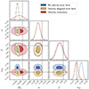 |
Fig. 2. MCMC results of the Hubble diagram fit using the three different methods to compute the PV covariance matrix described in Sect. 3. The fit was performed on one random realization. The dashed black lines show the simulation input value for each parameter. The blue contours show the posterior probability for each parameter when the PV covariance matrix is equal to zero, and PVs are not taken into account. The yellow contours show the results when the covariance matrix is just diagonal, assuming that σv = 250 km s−1. Finally, the red contours were obtained when we took into account the PV correlation and the covariance matrix was computed using the linear power spectrum. |
Results from the MCMC chains obtained on one realization.
In the case of M0, the PV modeling has a non-negligible impact. We observe a 4.5σ bias both when PVs are not accounted for or when neglecting their spatial correlations. However, Table 2 shows that when accounting for correlations, the uncertainty on M0 is about four times larger than the one obtained in the two other cases, making it compatible with its input value. This suggests that only using a diagonal term might not be sufficient to completely take into account the PVs’ impact in a low-redshift sample. We also notice that when using a diagonal term as well as the full covariance we recover the σM input value, while its value is increased when not taking into account PVs.
When computing the PV contribution to the error budget of M0 as
we find that the PVs are the main source of uncertainty for the M0 parameter with σM0, pv ∼ 0.013 mag.
In the next sections, we focus our study on the impact of PVs on the M0 parameter, as the impact on α and β is negligible, while σM is only a nuisance parameter in the fit. As was already mentioned, M0 is directly linked with the intercept of the Hubble diagram, aB, which is the parameter that has to be calibrated through the distance ladder to measure H0. Therefore, the effect of PVs on M0 estimation described in this section could bias the measurement of the Hubble constant when using SNe Ia.
4.2. M0 estimate and uncertainties
To see if the parameters values and uncertainties, in particular M0, were well estimated, we ran fits on all our 27 ZTF realizations. We ran the fit using iminuit8 (James & Roos 1975; Dembinski et al. 2020) to find the maximum of the likelihood. We checked that the results from iminuit are in agreement with the ones from the MCMC and used iminuit as a quicker solution to fit our 27 realizations. Figure 3 shows the results of these fits for M0. We highlight that even for the 27 realization fits, the results for α and β do not have any significant variation between the three methods. The additional results for these parameters are presented in Appendix C.
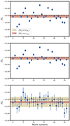 |
Fig. 3. M0 values obtained from the fit of the 27 realizations (realization number 8 is the one used in Fig. 2). The blue dots are the results of the fits with error bars from iminuit, while the dashed black line shows the M0 input value of the simulations. The shaded red area is centered on the mean M0 value ⟨M0⟩ obtained from the 27 realizations and it shows the uncertainty on ⟨M0⟩. The shaded yellow area is also centered on ⟨M0⟩, but shows the average uncertainty along the 27 realization results, ⟨σM02⟩1/2. Top panel: Fit without velocity error term. Middle panel: Fit with a velocity diagonal error term. Bottom panel: Fit with a full velocity covariance. |
The top panel of Fig. 3 shows our result for M0 obtained when we performed the fit without using any model for the velocity uncertainties. We measure that the standard deviation between the 27 realizations is STD(M0) = 0.014 mag, which is three to four times larger than the estimated uncertainty on the average ⟨σM02⟩1/2 = 0.004 mag. This result shows that uncertainties on M0 are clearly underestimated. The middle panel of Fig. 3 shows the same results when the contribution of PVs is modeled using the diagonal error term with σv = 250 km s−1. The resulting standard deviation over the 27 realizations is STD(M0) = 0.014 mag and the average uncertainty is ⟨σM02⟩1/2 = 0.004 mag. This result is identical to the previous case. It means that the diagonal error term is not sufficient to model the PV impact. Finally, the bottom panel of Fig. 3 shows the results for the case in which we use a complete velocity covariance matrix. We obtain a standard deviation of STD(M0) = 0.012 mag with a mean uncertainty of ⟨σM02⟩1/2 = 0.014 mag. In this last case, the standard deviation and uncertainty are compatible. Applying Eq. (19) used for one realization to the average uncertainties on M0, we retrieve a velocity contribution to the error budget on M0 of σM0, pv ∼ 0.013 mag.
We notice that in Fig. 3 the central value of ⟨M0⟩ is biased compared to the simulation input value with a difference of ΔM0 = ⟨M0⟩−M0, fid ∼ ( − 8 ± 2)×10−3 mag. This bias could be the result of correlations of the velocity field between the different mocks that originate from the same N-body simulated box. In order to study this effect, we ran a fit of the Hubble diagram without the effects of velocities by using the cosmological redshifts, zcos. The results are shown in Fig. 4. By correcting the velocities, the bias is reduced to ΔM0 ∼ ( − 2.0 ± 0.6)×10−3 mag. This effect could be explained by the fact that the realizations may be slightly correlated due to large modes inside the full OuterRim box. We understand the remaining small bias to be the first manifestation of the sample selection bias, also known as Malmquist bias, which arises from higher sampling of brighter objects when the distance increases. However, this bias does not affect the results on one measurement since it is compatible within 1σ with respect to the average uncertainty, ⟨σM02⟩1/2.
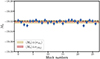 |
Fig. 4. Same as Fig. 3 but the redshifts and magnitudes have been corrected for velocity effects before fitting the Hubble diagram. |
The results of the comparison between the standard deviation of all the fitted parameters across the 27 ZTF survey realizations and the average uncertainties from the fit are summarized in Table 3. From these results, we find that in the case of the ZTF sample in the low-redshift regime, diagonal error terms are not sufficient to take into account the impact of PVs.
Comparison between the standard deviation of the parameters results computed across the 27 ZTF realizations and the average uncertainties obtained from the fit.
5. The intercept of the Hubble law in ZTF SN Ia DR2 data
The increasing uncertainty on M0 that we pointed out in the previous sections could have an impact on Hubble constant measurement from ZTF data (Dhawan et al. 2022). In such an analysis, H0 is computed using Eq. (2). The two parameters of Eq. (2) are the SNe Ia absolute magnitude, MB, which has to be calibrated using Cepheids or TRGB, and the intercept of the magnitude-redshift relation, aB. The latter is determined from the SNe Ia sample as

were DL is defined as DL = H0, fiddL, fid(z). This equation is a reformulation of Eq. (8) and the considerations we have made on M0 in the previous section are relevant for aB, since these two parameters are linearly linked as

Therefore, the corresponding uncertainty on H0 is
where σMB is the calibration uncertainty of the absolute magnitude of SNe Ia using calibrator stars (e.g., Cepheids or TRGB) and σ5aB is the uncertainty on 5aB. We ran a MCMC fit using this parameterization of the Hubble diagram on the ZTF SN Ia DR2 data.
The resulting contours of the MCMC for the three different methods of taking the PV into account are shown in Fig. 5, and the results are summarized in Table 4. The values of these results were blinded by the addition of a random offset to the SALT2 magnitude, mB. Therefore, the fitted parameters are shown as differences, Δp, relative to the results using a full covariance matrix. As is seen in the simulations, the parameters α and β and their corresponding uncertainties are the same for the three methods. The parameter of interest, aB, shifts by about ∼0.006 mag when the PV uncertainties are modeled by the full covariance matrix compared to the case in which PVs are not taken into account or modeled by a diagonal error term. This corresponds to an H0 shift of ∼1.0 km s−1 Mpc−1. The uncertainty on aB doubles, passing from σaB = 0.0018 mag to σaB = 0.0035 mag, when using the full covariance matrix compared to the two other methods. We also notice that the intrinsic scatter free parameter, σM, increases when using only a diagonal term or when not taking into account velocities because of its degeneracy with the diagonal terms of PV covariance.
 |
Fig. 5. MCMC results of the Hubble diagram fit for the ZTF SN Ia DR2 data using the three different methods of computing the PV covariance matrix described in Sect. 3. The symbols and colors are the same as in Fig. 2. The contours are shifted relative to the results obtained using a full covariance matrix for PVs. |
Results from the MCMC chains for the ZTF SN Ia DR2 data.
We find that, when taking into account PVs with the full covariance matrix, the uncertainty on aB corresponds to a contribution to the H0 error budget (Eq. 22) of σ5aB ≃ 0.0175 mag. Applying Eq. (19) to the uncertainty on 5aB, we compute that the velocity contribution is σ5aB, pv ∼ 0.015 mag, which is compatible with the result found on M0 with simulations. This could be translated as a contribution of σH0, pv ∼ 0.49 km s−1 Mpc−1 on the error on H0.
This result should be compared with the uncertainty on the calibrator term, σMB. In the last measurement of H0 combining TRGB and SNe Ia from ZTF (Dhawan et al. 2022), the uncertainty from calibrators could be decomposed in three terms that are described in Table 2 of the same paper. The first term is the SN Ia intrinsic scatter, the second term comes from the TRGB magnitude absolute calibration, and the last comes from the scatter of observed TRGB stars in SN Ia host galaxies. In this measurement, the error budget was dominated by the SN Ia intrinsic scatter of about ∼0.15 mag since there was only one SN Ia in the calibrator sample. In the future, the sample of calibrators is expected to grow up to ∼100, decreasing the contribution of SNe Ia scatter in calibrator samples to ∼0.01 mag. The same is expected for the scattering of TRGB stars in SNe Ia host galaxies with an expected uncertainty of ∼0.005 mag in future analysis. However, the TRGB absolute calibration uncertainty, which is about ∼0.038 mag, is driven by systematic uncertainties. It will be the major contribution to the H0 error budget in future measurements. It could be improved through the use of additional primary anchors and a better control over systematics (see Dhawan et al. 2022, Sect. 4) and is expected to be reduced to the level of ∼0.023 mag. To summarize, we could expect an uncertainty on MB in the range of σMB ∼ 0.026 − 0.040 mag. Therefore, considering the expected σMB and our result for the estimated σ5aB using the DR2 Hubble flow, from Eq. (22) we expect a relative uncertainty on H0 in the range of 1.4%−2.0% when the velocity covariance matrix is used. This is slightly higher than the relative uncertainty of 1.2%−1.9% that we computed when not using it.
6. Conclusion
In this paper, we have used the OuterRim N-body simulation described in Sect. 2 to obtain 27 realisations of the 6-year SN Ia sample of the ZTF survey including PV sample variance. Most of previous analyses (e.g., Betoule et al. 2014; Brout et al. 2019) have used a diagonal error matrix to account for the host-galaxy PVs. Due to the low redshift of the ZTF SN Ia DR2 sample, this approach is not valid to take into account the PV variance. The error bars on the M0 parameter are not compatible with the standard deviation computed across the 27 realisations, either when we did not take into account the PV term or when we used a diagonal matrix to describe PVs, as is shown in Sect. 4. To account for the PV sample variance in the M0 error budget, we need to use a full PV covariance matrix computed using the velocity power spectrum. This result, as in Davis et al. (2011), is an indication that even if in a previous SNe Ia low-z sample the PV correlation was negligible compared to the noise (Huterer et al. 2015), it is no longer valid for a large and homogeneous sample as the ZTF SN Ia DR2 sample.
We show that these PV correlations also have an impact on the measurement of H0, since they increase the uncertainty on the intercept of the Hubble diagram, aB. We tested this using ZTF SN Ia DR2 data, as is described in Sect. 5. The value of aB shifts by ΔaB ≃ 0.006, which corresponds to a shift in the H0 value of about ≃1.0 km s−1 Mpc−1. Moreover, the uncertainty on aB doubles when using the full PV covariance matrix compared to the other methods. The final contribution of aB in the H0 error budget is σ5aB = 0.0175. The PVs account for ≃0.015 mag in the value of σ5aB and ∼0.49 km s−1 Mpc−1 on the H0 error. This is slightly higher than the result of ∼0.31 km s−1 Mpc−1 obtained in Wu & Huterer (2017). Therefore, we conclude that neglecting the non-diagonal terms in the PV covariance matrix brings an underestimation of the uncertainty on the intercept of the Hubble diagram.
The uncertainty on H0 is currently dominated by the systematics from the calibrator sample. Future work on this source of systematics will reduce it, making it even more relevant to correctly take into account the PV contribution to the H0 error budget. Reconstruction methods that correct for PVs are a promising way to account for PV correlations. They should allow one to reduce the scatter due to PVs in the Hubble diagram, and thus suppress the PV sample variance issue. We have shown that an analysis using a full velocity covariance matrix ensures that PV effects are correctly accounted for. While not being competitive, the covariance matrix method can be used as a cross-check to investigate potential biases of the reconstruction methods, where the SN Ia redshifts are corrected using the velocities estimated from the density field (Carrick et al. 2015; Peterson et al. 2022; Carr et al. 2022).
Acknowledgments
Based on observations obtained with the Samuel Oschin Telescope 48-inch and the 60-inch Telescope at the Palomar Observatory as part of the Zwicky Transient Facility project. ZTF is supported by the National Science Foundation under Grants No. AST-1440341 and AST-2034437 and a collaboration including current partners Caltech, IPAC, the Weizmann Institute of Science, the Oskar Klein Center at Stockholm University, the University of Maryland, Deutsches Elektronen-Synchrotron and Humboldt University, the TANGO Consortium of Taiwan, the University of Wisconsin at Milwaukee, Trinity College Dublin, Lawrence Livermore National Laboratories, IN2P3, University of Warwick, Ruhr University Bochum, Northwestern University and former partners the University of Washington, Los Alamos National Laboratories, and Lawrence Berkeley National Laboratories. Operations are conducted by COO, IPAC, and UW. SED Machine is based upon work supported by the National Science Foundation under Grant No. 1106171 The project leading to this publication has received funding from Excellence Initiative of Aix-Marseille University – A*MIDEX, a French “Investissements d’Avenir” program (AMX-20-CE-02 – DARKUNI). This work has been carried out thanks to the support of the DEEPDIP ANR project (ANR-19-CE31-0023). This work received support from the French government under the France 2030 investment plan, as part of the Initiative d’Excellence d’Aix-Marseille Université – A*MIDEX (AMX-19-IET-008 – IPhU). This project has received funding from the European Research Council (ERC) under the European Union’s Horizon 2020 research and innovation programme (grant agreement n°759194 – USNAC). This project has received funding from the European Research Council (ERC) under the European Union’s Horizon 2020 research and innovation programme (grant agreement n°759194 – USNAC) This work has been supported by the Agence Nationale de la Recherche of the French government through the program ANR-21-CE31-0016-03. This work has been supported by the research project grant “Understanding the Dynamic Universe” funded by the Knut and Alice Wallenberg Foundation under Dnr KAW 2018.0067, Vetenskapsrådet, the Swedish Research Council, project 2020-03444 and the G.R.E.A.T. research environment, project number 2016-06012. L.G. acknowledges financial support from the Spanish Ministerio de Ciencia e Innovación (MCIN) and the Agencia Estatal de Investigación (AEI) 10.13039/501100011033 under the PID2020-115253GA-I00 HOSTFLOWS project, from Centro Superior de Investigaciones Científicas (CSIC) under the PIE project 20215AT016 and the program Unidad de Excelencia María de Maeztu CEX2020-001058-M, and from the Departament de Recerca i Universitats de la Generalitat de Catalunya through the 2021-SGR-01270 grant. G.D. is supported by the H2020 European Research Council grant no. 758638. T.E.M.B. acknowledges financial support from the Spanish Ministerio de Ciencia e Innovación (MCIN), the Agencia Estatal de Investigación (AEI) 10.13039/501100011033, and the European Union Next Generation EU/PRTR funds under the 2021 Juan de la Cierva program FJC2021-047124-I and the PID2020-115253GA-I00 HOSTFLOWS project, from Centro Superior de Investigaciones Científicas (CSIC) under the PIE project 20215AT016, and the program Unidad de Excelencia María de Maeztu CEX2020-001058-M. U.B. and J.H.T. are supported by the H2020 European Research Council grant no. 758638.
References
- Amenouche, M., Rosnet, P., Smith, M., et al. 2025, A&A, 694, A3 (ZTF DR2 SI) [NASA ADS] [CrossRef] [EDP Sciences] [Google Scholar]
- Barbary, K., Bailey, S., Barentsen, G., et al. 2023, https://doi.org/10.5281/zenodo.8091892 [Google Scholar]
- Bellm, E. C., Kulkarni, S. R., Graham, M. J., et al. 2019, PASP, 131, 018002 [Google Scholar]
- Betoule, M., Kessler, R., Guy, J., et al. 2014, A&A, 568, A22 [NASA ADS] [CrossRef] [EDP Sciences] [Google Scholar]
- Blagorodnova, N., Neill, J. D., Walters, R., et al. 2018, PASP, 130, 035003 [Google Scholar]
- Brout, D., Scolnic, D., Kessler, R., et al. 2019, ApJ, 874, 150 [NASA ADS] [CrossRef] [Google Scholar]
- Brout, D., Scolnic, D., Popovic, B., et al. 2022, ApJ, 938, 110 [NASA ADS] [CrossRef] [Google Scholar]
- Carr, A., Davis, T. M., Scolnic, D., et al. 2022, PASA, 39, e046 [NASA ADS] [CrossRef] [Google Scholar]
- Carreres, B., Bautista, J. E., Feinstein, F., et al. 2023, A&A, 674, A194 [NASA ADS] [CrossRef] [EDP Sciences] [Google Scholar]
- Carrick, J., Turnbull, S. J., Lavaux, G., & Hudson, M. J. 2015, MNRAS, 450, 317 [Google Scholar]
- Cooray, A., & Caldwell, R. R. 2006, Phys. Rev. D, 73, 103002 [CrossRef] [Google Scholar]
- DESI Collaboration (Aghamousa, A., et al.) 2016, ArXiv e-prints [arXiv:1611.00036] [Google Scholar]
- Davis, T. M., Hui, L., Frieman, J. A., et al. 2011, ApJ, 741, 67 [NASA ADS] [CrossRef] [Google Scholar]
- Dekany, R., Smith, R. M., Riddle, R., et al. 2020, PASP, 132, 038001 [NASA ADS] [CrossRef] [Google Scholar]
- Dembinski, H., Ongmongkolkul, P., Deil, C., et al. 2020, https://doi.org/10.5281/zenodo.3949207 [Google Scholar]
- Dhawan, S., Goobar, A., Johansson, J., et al. 2022, ApJ, 934, 185 [NASA ADS] [CrossRef] [Google Scholar]
- Graham, M. J., Kulkarni, S. R., Bellm, E. C., et al. 2019, PASP, 131, 078001 [Google Scholar]
- Graziani, R., Courtois, H. M., Lavaux, G., et al. 2019, MNRAS, 488, 5438 [NASA ADS] [CrossRef] [Google Scholar]
- Guy, J., Astier, P., Baumont, S., et al. 2007, A&A, 466, 11 [NASA ADS] [CrossRef] [EDP Sciences] [Google Scholar]
- Guy, J., Sullivan, M., Conley, A., et al. 2010, A&A, 523, A7 [NASA ADS] [CrossRef] [EDP Sciences] [Google Scholar]
- Heitmann, K., Finkel, H., Pope, A., et al. 2019, ApJS, 245, 16 [NASA ADS] [CrossRef] [Google Scholar]
- Howlett, C., Staveley-Smith, L., Elahi, P. J., et al. 2017, MNRAS, 471, 3135 [NASA ADS] [CrossRef] [Google Scholar]
- Hui, L., & Greene, P. B. 2006, Phys. Rev. D, 73, 123526 [NASA ADS] [CrossRef] [Google Scholar]
- Huterer, D., Shafer, D. L., & Schmidt, F. 2015, JCAP, 2015, 033 [Google Scholar]
- James, F., & Roos, M. 1975, Comput. Phys. Commun., 10, 343 [Google Scholar]
- Johnson, A., Blake, C., Koda, J., et al. 2014, MNRAS, 444, 3926 [NASA ADS] [CrossRef] [Google Scholar]
- Kenworthy, W. D., Riess, A. G., Scolnic, D., et al. 2022, ApJ, 935, 83 [NASA ADS] [CrossRef] [Google Scholar]
- Kessler, R., Becker, A. C., Cinabro, D., et al. 2009, ApJS, 185, 32 [Google Scholar]
- Kim, Y. L., Rigault, M., Neill, J. D., et al. 2022, PASP, 134, 024505 [NASA ADS] [CrossRef] [Google Scholar]
- Lai, Y., Howlett, C., & Davis, T. M. 2023, MNRAS, 518, 1840 [Google Scholar]
- Laureijs, R., Amiaux, J., Arduini, S., et al. 2011, ArXiv e-prints [arXiv:1110.3193] [Google Scholar]
- Lavaux, G., & Hudson, M. J. 2011, MNRAS, 416, 2840 [Google Scholar]
- Lewis, A., Challinor, A., & Lasenby, A. 2000, ApJ, 538, 473 [Google Scholar]
- Lilow, R., & Nusser, A. 2021, MNRAS, 507, 1557 [NASA ADS] [CrossRef] [Google Scholar]
- LSST Science Collaboration (Abell, P. A., et al.) 2009, ArXiv e-prints [arXiv:0912.0201] [Google Scholar]
- Masci, F. J., Laher, R. R., Rusholme, B., et al. 2019, PASP, 131, 018003 [Google Scholar]
- Nicolas, N., Rigault, M., Copin, Y., et al. 2021, A&A, 649, A74 [NASA ADS] [CrossRef] [EDP Sciences] [Google Scholar]
- Peebles, P. J. E. 1980, The Large-scale Structure of the Universe (Princeton: Princeton University Press) [Google Scholar]
- Perley, D. A., Fremling, C., Sollerman, J., et al. 2020, ApJ, 904, 35 [NASA ADS] [CrossRef] [Google Scholar]
- Peterson, E. R., Kenworthy, W. D., Scolnic, D., et al. 2022, ApJ, 938, 112 [NASA ADS] [CrossRef] [Google Scholar]
- Planck Collaboration VI. 2020, A&A, 641, A6 [NASA ADS] [CrossRef] [EDP Sciences] [Google Scholar]
- Riess, A. G., Yuan, W., Macri, L. M., et al. 2022, ApJ, 934, L7 [NASA ADS] [CrossRef] [Google Scholar]
- Rigault, M., Neill, J. D., Blagorodnova, N., et al. 2019, A&A, 627, A115 [NASA ADS] [CrossRef] [EDP Sciences] [Google Scholar]
- Rigault, M., Smith, M., Goobar, A., et al. 2025, A&A, 694, A1 (ZTF DR2 SI) [NASA ADS] [CrossRef] [EDP Sciences] [Google Scholar]
- Said, K., Colless, M., Magoulas, C., Lucey, J. R., & Hudson, M. J. 2020, MNRAS, 497, 1275 [NASA ADS] [CrossRef] [Google Scholar]
- Scolnic, D., & Kessler, R. 2016, ApJ, 822, L35 [Google Scholar]
- Scolnic, D., Riess, A. G., Wu, J., et al. 2023, ArXiv e-prints [arXiv:2304.06693] [Google Scholar]
- Smith, M., Rigault, M., et al. 2025, A&A, in prep. (ZTF DR2 SI) [Google Scholar]
- Soumagnac, M. T., Nugent, P., Knop, R. A., et al. 2024, ArXiv e-prints [arXiv:2405.03857] [Google Scholar]
- Tripp, R. 1998, A&A, 331, 815 [NASA ADS] [Google Scholar]
- Turner, R. J., Blake, C., & Ruggeri, R. 2022, ArXiv e-prints [arXiv:2207.03707] [Google Scholar]
- Wu, H.-Y., & Huterer, D. 2017, MNRAS, 471, 4946 [CrossRef] [Google Scholar]
Appendix A: Discussion on correlation between sub-boxes
We produced several realizations of ZTF by cutting a single OuterRim simulation into non-overlapping sub-boxes. However, PVs are coherent over large scales, so these realizations are not fully independent. We estimated the correlation function between PVs inside different sub-boxes as a function of scale, shown in Fig. A.1. We see that the absolute value of the correlation between two SN Ia host that pass the redshift cut of z < 0.06, that corresponds to a distance of ∼180 Mpc.h−1 in our fiducial cosmology, in two different sub-boxes is ∼0.016. The correlation between velocities at a distance from one sub-box center to another sub-center is ∼0.008. From the comparison of these values to the average correlation absolute value between two SNe Ia that pass the redshift cut inside one mock ∼0.14, we conclude that the correlation between the sub-boxes can be mostly neglected. However, we see in Sect. 4.2 that a part of the small bias observed on M0 could be explained by the effect of the velocity correlation across the different sub-boxes since removing velocities seems to lower the bias.
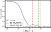 |
Fig. A.1. Peculiar velocity correlation absolute value between two galaxies on the same line-of-sight in function of the radial separation. The vertical dotted lines indicate the distance corresponding to the redshift cut z ∼ 0.06 (red), the minimum distance between two SNe Ia that pass the redshift cut in two different sub-boxes (green) and the distance between two sub-boxes center (yellow). |
Appendix B: Testing the assumptions in the covariance computation
We assert the robustness of the analysis by testing it against the assumptions we have done to compute the velocity covariance. In particular, the input cosmological parameters in Appendix B.1 and the chosen maximum scale in Appendix B.2. During the analysis we have assumed a linear power spectrum  in order to compute the complete velocity covariance. This choice is done because in this work we are not measuring the parameters of the cosmological model. Here, we are analyzing systematics and the choice of the power spectrum is a second order effect. Therefore, for simplicity we choose to utilize the linear power spectrum. We highlight that we perform few test in order to assess the impact of the power spectrum choice. The results, which are not shown in the paper, are that changing the power spectrum does not change at all the final results presented in this work. For an extensive description on the non linear power spectrum models and the differences with the linear one see Carreres et al. (2023) and references therein.
B.1. Changing the input cosmology
As a first test we perform the Hubble diagram fit on one random realization changing the input cosmology in the covariance computation respect to the one presented in Sect. 2. The results of the MCMC chains are shown in Fig. B.1. The figure shows that changing H0 and the density of cold dark matter, Ωc, does not change the results of the Hubble diagram fit. Furthermore, Fig. B.1 table shows that the recovered parameter values for the three different cosmology are exactly the same within the uncertainties. Therefore, we conclude that the results presented in this work are independent from the choice of the cosmological parameters in the velocity covariance computation.
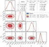 |
Fig. B.1. MCMC results of the Hubble diagram fit using three different values input cosmologies to compute the power spectrum Pθθ for the complete velocity covariance. The fit is performed on the same realization shown in Fig. 2. The dashed black lines show the simulation input value for each parameter. The baseline refers to OuterRim cosmology as described in Sect. 2. The table shows the median posterior probability, the fitted value, for each parameter and the relative error. |
B.2. Changing the maximum scale
We perform the Hubble diagram fit on one random realization changing the maximum scale kmax in the velocity covariance computation. Figure B.2 shows the result of this test. We find that changing kmax does not change the contours with respect to the baseline choice of kmax = 0.2 h−1Mpc done in the analysis. As in the previous section, Fig. B.2 shows that the recovered parameter values are exactly the same within the uncertainties. We conclude that for the purpose of systematic assessment we are independent from the choice of the maximum scale.
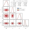 |
Fig. B.2. MCMC results of the Hubble diagram fit using three different values of kmax to compute the power spectrum Pθθ for the complete velocity covariance. The fit is performed on the same realization shown in Fig. 2. The dashed black lines show the simulation input value for each parameter. The baseline refers to kmax = 0.2 h−1Mpc as described in Sect. 3. The table shows the median posterior probability, the fitted value, for each parameter and the relative error. |
Appendix C: Scatter of α, β, and σM across the 27 ZTF realizations
In Sect. 4 we emphasized that using or not the PVs covariance does not affect the fit of the α and β parameters. This is what we can see in more details in Figs. C.1 and C.2. The figures show the results for these parameters across the 27 ZTF realizations. On these figures we do not notice any significant changes. However, we see that the values of α and β are slightly bias, as for M0, this could be an effect of the sample selection.
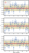 |
Fig. C.1. α values obtained from the fit of the 27 realizations. The dashed black lines show the simulation input value of the α parameter. Top panel: Fit without velocity error term. Middle panel: Fit with a velocity diagonal error term. Bottom panel: Fit with a full velocity covariance. |
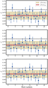 |
Fig. C.2. β values obtained from the fit of the 27 realizations. The dashed black lines show the simulation input value of the β parameter. Top panel: Fit without velocity error term. Middle panel: Fit with a velocity diagonal error term. Bottom panel: Fit with a full velocity covariance. |
Figure C.3 shows the same results for the σM parameter, which represents the non-modeled scattering of the Hubble residuals. We can see that including PVs as diagonal or full covariance matrix reduces the recovered value of σM. It can be explained by the fact that this parameter will absorb the PV scattering if it is not modeled.
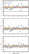 |
Fig. C.3. σM values obtained from the fit of the 27 realizations. The dashed black lines show the simulation input value of the σM parameter. Top panel: Fit without velocity error term. Mid panel: Fit with a velocity diagonal error term. Bottom panel: Fit with a full velocity covariance. |
All Tables
Comparison between the standard deviation of the parameters results computed across the 27 ZTF realizations and the average uncertainties obtained from the fit.
All Figures
|
Fig. 1. Comparison of the angular and redshift distributions of the SNe Ia from the simulation and from the ZTF SN Ia DR2 data. Top panel: Angular positions of simulated SNe Ia from one mock (in blue) and from the DR2 data (in red). Bottom panel: Redshift distribution averaged over the 27 mocks and rescaled for the difference in the duration of the survey (in blue) compared to the DR2 redshift distribution (in red). |
| In the text | |
|
Fig. 2. MCMC results of the Hubble diagram fit using the three different methods to compute the PV covariance matrix described in Sect. 3. The fit was performed on one random realization. The dashed black lines show the simulation input value for each parameter. The blue contours show the posterior probability for each parameter when the PV covariance matrix is equal to zero, and PVs are not taken into account. The yellow contours show the results when the covariance matrix is just diagonal, assuming that σv = 250 km s−1. Finally, the red contours were obtained when we took into account the PV correlation and the covariance matrix was computed using the linear power spectrum. |
| In the text | |
|
Fig. 3. M0 values obtained from the fit of the 27 realizations (realization number 8 is the one used in Fig. 2). The blue dots are the results of the fits with error bars from iminuit, while the dashed black line shows the M0 input value of the simulations. The shaded red area is centered on the mean M0 value ⟨M0⟩ obtained from the 27 realizations and it shows the uncertainty on ⟨M0⟩. The shaded yellow area is also centered on ⟨M0⟩, but shows the average uncertainty along the 27 realization results, ⟨σM02⟩1/2. Top panel: Fit without velocity error term. Middle panel: Fit with a velocity diagonal error term. Bottom panel: Fit with a full velocity covariance. |
| In the text | |
|
Fig. 4. Same as Fig. 3 but the redshifts and magnitudes have been corrected for velocity effects before fitting the Hubble diagram. |
| In the text | |
|
Fig. 5. MCMC results of the Hubble diagram fit for the ZTF SN Ia DR2 data using the three different methods of computing the PV covariance matrix described in Sect. 3. The symbols and colors are the same as in Fig. 2. The contours are shifted relative to the results obtained using a full covariance matrix for PVs. |
| In the text | |
|
Fig. A.1. Peculiar velocity correlation absolute value between two galaxies on the same line-of-sight in function of the radial separation. The vertical dotted lines indicate the distance corresponding to the redshift cut z ∼ 0.06 (red), the minimum distance between two SNe Ia that pass the redshift cut in two different sub-boxes (green) and the distance between two sub-boxes center (yellow). |
| In the text | |
|
Fig. B.1. MCMC results of the Hubble diagram fit using three different values input cosmologies to compute the power spectrum Pθθ for the complete velocity covariance. The fit is performed on the same realization shown in Fig. 2. The dashed black lines show the simulation input value for each parameter. The baseline refers to OuterRim cosmology as described in Sect. 2. The table shows the median posterior probability, the fitted value, for each parameter and the relative error. |
| In the text | |
|
Fig. B.2. MCMC results of the Hubble diagram fit using three different values of kmax to compute the power spectrum Pθθ for the complete velocity covariance. The fit is performed on the same realization shown in Fig. 2. The dashed black lines show the simulation input value for each parameter. The baseline refers to kmax = 0.2 h−1Mpc as described in Sect. 3. The table shows the median posterior probability, the fitted value, for each parameter and the relative error. |
| In the text | |
|
Fig. C.1. α values obtained from the fit of the 27 realizations. The dashed black lines show the simulation input value of the α parameter. Top panel: Fit without velocity error term. Middle panel: Fit with a velocity diagonal error term. Bottom panel: Fit with a full velocity covariance. |
| In the text | |
|
Fig. C.2. β values obtained from the fit of the 27 realizations. The dashed black lines show the simulation input value of the β parameter. Top panel: Fit without velocity error term. Middle panel: Fit with a velocity diagonal error term. Bottom panel: Fit with a full velocity covariance. |
| In the text | |
|
Fig. C.3. σM values obtained from the fit of the 27 realizations. The dashed black lines show the simulation input value of the σM parameter. Top panel: Fit without velocity error term. Mid panel: Fit with a velocity diagonal error term. Bottom panel: Fit with a full velocity covariance. |
| In the text | |
Current usage metrics show cumulative count of Article Views (full-text article views including HTML views, PDF and ePub downloads, according to the available data) and Abstracts Views on Vision4Press platform.
Data correspond to usage on the plateform after 2015. The current usage metrics is available 48-96 hours after online publication and is updated daily on week days.
Initial download of the metrics may take a while.