| Issue |
A&A
Volume 697, May 2025
ZTF SN Ia DR2
|
|
|---|---|---|
| Article Number | A125 | |
| Number of page(s) | 16 | |
| Section | Cosmology (including clusters of galaxies) | |
| DOI | https://doi.org/10.1051/0004-6361/202452578 | |
| Published online | 12 May 2025 | |
ZTF SN Ia DR2: Improved SN Ia colors through expanded dimensionality with SALT3+
1
The Oskar Klein Centre, Department of Physics, Stockholm University, SE-106 91 Stockholm, Sweden
2
Institute for Astronomy, University of Hawai’i, 640 N. Aohoku Pl., Hilo, HI 96720, USA
3
Kavli Institute for Cosmological Physics, University of Chicago, Chicago, IL 60637, USA
4
Department of Astronomy and Astrophysics, University of Chicago, Chicago, IL 60637, USA
5
School of Physics, Trinity College Dublin, The University of Dublin, Dublin 2, Ireland
6
Institute of Astronomy, Madingley Rd, Cambridge CB3 0HA, United Kingdom
7
Institute of Space Sciences (ICE, CSIC), Campus UAB, Carrer de Can Magrans s/n, E-08193 Barcelona, Spain
8
Institut d’Estudis Espacials de Catalunya (IEEC), 08860 Castelldefels (Barcelona), Spain
9
Univ. Lyon, Univ. Claude Bernard Lyon 1, CNRS, IP2I Lyon/IN2P3, UMR 5822, F-69622 Villeurbanne, France
10
Department of Physics, Lancaster University, Lancs LA1 4YB, UK
11
Lawrence Berkeley National Laboratory, 1 Cyclotron Road MS 50B-4206, Berkeley, CA 94720, USA
12
Department of Astronomy, University of California, Berkeley, 501 Campbell Hall, Berkeley, CA 94720, USA
13
Institut für Physik, Humboldt-Universität zu Berlin, Newtonstr. 15, 12489 Berlin, Germany
14
Université Clermont Auvergne, CNRS/IN2P3, LPCA, F-63000 Clermont-Ferrand, France
15
The Oskar Klein Centre, Department of Astronomy, Stockholm University, SE-106 91 Stockholm, Sweden
16
Nordic Optical Telescope, Rambla José Ana Fernández Pérez 7, ES-38711 Breña Baja, Spain
17
IPAC, California Institute of Technology, 1200 E. California Boulevard, Pasadena CA 91125, USA
18
Caltech Optical Observatories, California Institute of Technology, Pasadena, CA 91125, USA
19
Aix Marseille Université, CNRS/IN2P3, CPPM, Marseille, France
⋆ Corresponding author: This email address is being protected from spambots. You need JavaScript enabled to view it.
Received:
11
October
2024
Accepted:
7
March
2025
Abstract
Context. Type Ia supernovae (SNe Ia) are a key probe in modern cosmology, as they can be used to measure luminosity distances at gigaparsec scales. Models of their light curves are used to project heterogeneous observed data onto a common basis for analysis.
Aims. The SALT model currently used for SN Ia cosmology describes SNe as having two sources of variability, accounted for by a color parameter c, and a “stretch” parameter x1. We extend the model to include an additional parameter we label x2, to investigate the cosmological impact of currently unaddressed light-curve variability.
Methods. We constructed a new SALT model, that we dub “SALT3+”. This model was trained by an improved version of the SALTshaker code, using training data combining a selection of the second data release of cosmological SNe Ia from the Zwicky Transient Facility and the existing SALT3 training compilation.
Results. We find additional, coherent variability in supernova light curves beyond SALT3. Most of this variation can be described as phase-dependent variation in g − r and r − i color curves, correlated with a boost in the height of the secondary maximum in i-band. These behaviors correlate with spectral differences, particularly in line velocity. We find that fits with the existing SALT3 model tend to address this excess variation with the color parameter, leading to less informative measurements of supernova color. We find that neglecting the new parameter in light-curve fits leads to a trend in Hubble residuals with x2 of 0.039 ± 0.005 mag, representing a potential systematic uncertainty. However, we find no evidence of a bias in current cosmological measurements.
Conclusions. We conclude that extended SN Ia light-curve models promise mild improvement in the accuracy of color measurements, and corresponding cosmological precision. However, models with more parameters are unlikely to substantially affect current cosmological results.
Key words: methods: data analysis / supernovae: general / distance scale
© The Authors 2025
 Open Access article, published by EDP Sciences, under the terms of the Creative Commons Attribution License (https://creativecommons.org/licenses/by/4.0), which permits unrestricted use, distribution, and reproduction in any medium, provided the original work is properly cited.
This article is published in open access under the Subscribe to Open model. This email address is being protected from spambots. You need JavaScript enabled to view it. to support open access publication.
1. Introduction
Type Ia supernovae are standardizable candles that allow precision measurements of cosmological distances across cosmic history at gigaparsec scales. As a homogeneous population of objects sourced from the thermonuclear explosion of a white dwarf, they show extraordinary spectroscopic and photometric consistency. Measurements of Type Ia supernovae (SNe Ia) from photometric surveys are a key ingredient of modern efforts to measure the properties of dark energy (LSST Dark Energy Science Collaboration 2018; Hounsell et al. 2018; Brout et al. 2022a; Rubin et al. 2023; Vincenzi et al. 2024). Their use as cosmological indicators relies on the use of a light-curve model serving several purposes: (a) to interpolate samples from multiple surveys onto a common phase and wavelength basis for comparison, (b) reduce the dimensionality of the data, and (c) parameterize the variability of the underlying data for use in standardization and cosmology analysis.
The Spectral Adaptive Light-curve Template (SALT) model was first published in Guy et al. (2005), and was substantially updated in Guy et al. (2007). With ongoing improvements to sample size and calibration, SALT2 was the primary model for every published measurement of the dark-energy equation-of-state parameter w using SNe Ia between 2011 and 2022. The model was updated in Guy et al. (2010) and Betoule et al. (2014). A more recent revision (SALT2.T21) was presented by Taylor et al. (2021). In Kenworthy et al. (2021) (hereafter K21) a new training code was developed, the model error term was redefined, and the training sample was expanded by a factor of 2.5, resulting in the SALT3 model (here referred to as SALT3.K21). Further work from Dai et al. (2023) and Taylor et al. (2023) has constrained systematics of the SALTShaker training code and SALT3.K21 model. The Union 3/UNITY 1.5 analysis (Rubin et al. 2023), as well as the 5 year analysis of the Dark Energy Survey’s supernova experiment (Taylor et al. 2023; Vincenzi et al. 2024), used SALT3 for the first time in a cosmological analysis. Jones et al. (2023) and Taylor et al. (2024) also explored variation in light curves between different host-galaxy types using the SALT framework.
The SALT framework is distinguished by several key elements from other SN Ia models available in the community (e.g. MLCS2k2; Jha et al. 2007, BayeSN; Mandel et al. 2011; Thorp et al. 2021; Grayling et al. 2024, SnooPy; Burns et al. 2014, 2018, SNEMO; Saunders et al. 2018, and SUGAR; Léget et al. 2020). The model is fully empirical, by construction prioritizing the parametrization of SN Ia photometric diversity over links to specific physical mechanisms e.g. spectroscopic lines, theoretical simulations, or parametrizations of dust extinction. Spectroscopic data is included in model construction to ensure rest-frame modelled photometry is reliable across the redshift range and prevent deconvolution noise1, but is explicitly downweighted compared to photometric data. SALT aims to avoid making assumptions about cosmology or underlying populations in model construction. Instead SALT prioritizes homogenizing and reducing diverse measured photometry to a form suitable for further analysis by frameworks such as Bayesian Estimation Applied to Multiple Species with Bias Correction (BEAMS/BBC) (Kunz et al. 2007; Kessler & Scolnic 2017), Unified Nonlinear Inference for Type-Ia cosmologY (UNITY) (Rubin et al. 2015, 2023), Dust2Dust (Popovic et al. 2023), and others (e.g. March et al. 2011; Shariff et al. 2016; Mandel et al. 2017; Feeney et al. 2018; Rahman et al. 2022; Wojtak et al. 2023). These frameworks may be better suited to make and evaluate decisions about selection, cosmology, and population demographics. Finally, as an empirical model, SALT is constructed by reference to a training sample of SN Ia data. The construction of this sample has emphasized the use of data from a diversity of carefully collected SN Ia surveys. By doing so, we aim to include demographics similar to samples typically used for cosmology, across a range of filters, cadences, calibrations, and redshifts. By sample-matching in this way, both “known unknown” and “unknown unknown” systematics can be reduced.
SALT models as published rely on a single parameter for the phase-dependent variation of the SN Ia light curve and a single color parameter accounting for intrinsic and/or extrinsic reddening. The intrinsic variation parameter x1 is associated with the light-curve “stretch”, a change in the decay time of the light curve post-maximum. The stretch of SNe Ia has been associated with the amount of 56Ni produced in the thermonuclear explosion (Phillips 1993; Kasen & Woosley 2007). The decay of this unstable isotope heats the ejecta, increasing the luminosity of the explosion as well as delaying ionization transitions of iron-group elements, increasing opacity and broadening the light curve. However theoretical evidence suggests that other factors may also affect the light curve of the supernova.
Observationally, work by Saunders et al. (2018) and Rubin (2020) suggest that SN Ia phase-dependent spectrophotometry is more complicated than can be modeled by a single intrinsic parameter. Rigault et al. (2025a) shows deviations of light-curve residuals from SALT fits in the ZTF DR2 sample, suggesting that the time-dependence of SN Ia colors are not fully addressed by SALT. Hayden et al. (2019) split the SALT2 model into pre- and post-maximum components (extending the dimensionality by one). They found that the pre-maximum light curves of SNe Ia seemed to be more effective in standardization than post-maximum. Fully trained SN Ia models, including SNEMO (Saunders et al. 2018) and SUGAR (Léget et al. 2020) have included higher-dimensionality variants. However both these models were exclusively developed with spectrophotometric data from the SNFactory (Aldering et al. 2002). This unique data gave these models excellent coverage over the wavelength domain of the SNIFS instrument (∼3300 − 8600 Å). However use of these models for cosmology analysis is obstructed by two primary issues. Rose et al. (2020) found that the majority of available SN Ia photometry was unable to constrain the 7-dimensional SNEMO7 model due to the size of the parameter space, with substantial correlations in fitted parameters that obstruct cosmological analysis. Further, the low redshift of the SNFactory the model is possibly susceptible to evolving demographic biases with redshift. Rose et al. (2020) therefore suggested a lower-dimensionality model would likely be most useful. Therefore, it is desirable to make available a SN Ia model incorporating the broad demographics and wavelength coverage of the SALT training samples, with a lower dimensionality than SNEMO7 to allow more robust fits against multi-band SN Ia photometry of typical observation cadence. Additionally, a higher dimensional BayeSN model was also included in the appendix of Mandel et al. (2022). Beyond any utility in standardization, a higher-dimensional SALT model may be important for use in bias correction simulations using BBC, or equivalently, selection integrals in UNITY.
Here we used the SALTshaker code presented in K21 to train a model we label SALT3+, a two-dimensional model of phase-dependent SN Ia variability. To efficiently constrain phase-dependent behavior, we incorporated data from the Zwicky Transient Facility (Bellm et al. 2019; Graham et al. 2019) in concert with the compilation of training data already assembled, which we discuss in Sect. 2. We present updates to the SALTshaker code as well as the full description of the SALT3+ model in Sect. 3. Lastly, we discuss our results and conclusions in Sects. 4 and 5.
2. Data
We used the original compilation of data assembled in K21, adding spectroscopically typed SNe Ia from the second data release of ZTF SNe Ia, ZTF SN Ia DR2 (Rigault et al. 2025b) to train our light-curve model. Combining these data increased the total number of photometric epochs and spectra by ∼50%. In Fig. 1, we show the available data as a function of phase and wavelength for K21 as well as the ZTF sample. As we examine host galaxy relations in our analysis in Sect. 4.3, we used host-galaxy masses from Pantheon+ (Brout et al. 2022a) for the K21 compilation where available, and estimates from the ZTF DR2 for ZTF objects (Smith et al., in prep.).
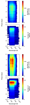 |
Fig. 1. Density of spectroscopic and photometric data from training samples as a function of wavelength. A photometric epoch is considered to cover a given wavelength bin if the wavelength is within the FWHM of the filter in the rest-frame. Bin sizes are dictated by the underlying resolution of the SED model. Top two panels show data density with the K21 compilation alone, lower two panels show the K21+ZTF compilation. |
2.1. K21 compilation
The K21 compilation was described in Kenworthy et al. (2021). The compilation built on the sample used by the Joint Light-curve Analysis to train the SALT2 model (Betoule et al. 2014), and incorporated data from many of the largest available surveys for cosmological SNe. In total, it consists of 1048 SNe from the Sloan Digital Sky Survey (SDSS; Holtzman et al. 2008; Kessler et al. 2009a; Sako et al. 2018), the Supernova Legacy Survey (SNLS; Astier et al. 2006, with spectra from Walker et al. 2011; Balland et al. 2018 and private communication with M. Betoule, C. Balland), the Calan-Tololo Survey (Hamuy et al. 1996), the Center for Astrophysics surveys (CfA; Riess et al. 1999; Jha et al. 2006; Hicken et al. 2009, 2012), the Carnegie Supernova Project (Krisciunas et al. 2017), the Foundation Supernova Survey (Foley et al. 2018; Jones et al. 2019), the Pan-STARRS Medium Deep Survey (Rest et al. 2014; Scolnic et al. 2018), and the Dark Energy Survey (Abbott et al. 2019). This sample was used to train the first published SALT3 models. Since then new calibration solutions for the photometric systems have been made available in Brout et al. (2022b)2, and the models trained here have made use of these recalibrations.
Following the suggestions of Vincenzi et al. (2024) as well as Taylor et al. (2023), we excluded all U-band light curves from the sample due to calibration uncertainties (see also earlier discussion in Kessler et al. 2009a; Krisciunas et al. 2013). This change affects 97 SNe in the data, principally from the CfA surveys.
2.2. ZTF DR2
As described in Rigault et al. (2025b), the second data release of cosmological SNe from the ZTF collaboration (Bellm et al. 2019; Graham et al. 2019; Masci et al. 2019; Dekany et al. 2020) consists of 3627 spectroscopically classified SNe Ia primarily obtained from the Bright Transient Survey (Fremling et al. 2020; Perley et al. 2020), a magnitude-limited sample of extragalactic transients in the northern sky. All SNe in this data release were observed between April 2018 and December 2020. We used the gri band photometry to train our models. The calibration solution of the ZTF SN sample is still a work in progress, and the models presented here will thus have unbudgeted calibration uncertainties of > 0.01 mag.
To ensure each individual ZTF light curve used had sufficient coverage to examine the time-dependent behavior beyond x1, we included substantial light-curve quality cuts. These cuts on ZTF data are stricter than those applied to the K21 sample, and we chose not to apply them to the previously compiled data. The primary reason for this choice is that the SALT model philosophy, as discussed in Sect. 1, prioritizes carefully collected yet heterogeneous data. Applying these stricter cuts to the previous training sample would have substantially reduced the amount of non-ZTF data available in the training, causing the model to prioritize explaining the ZTF data. Analogy here with principal component analysis is useful. When a PCA is performed, the vectors found depend on the importance of different modes in the data. As that distribution shifts, the relative importance of different modes shifts as well. Phenomenology is then allocated to different component vectors. Further discussion of the issues of imbalanced data-sets can be found in Fernández et al. (2018). The overall ZTF sample includes ∼1600 SNe passing the K21 quality cuts with host-redshift data, larger than the entirety of the previous training sample. Including this amount of data naively would result in a model strongly weighted towards characterizing the ZTF data. Applying such a model to high-redshift SNe, measured in different bands and with possibly divergent demographics, might fail to capture relevant information. While these effects can be simulated using validation pipelines such as that presented in Dai et al. (2023), preventing the ZTF data from becoming a majority of measured light curves is a safer solution. Accordingly we required, labeling phase relative to SALT2 maximum light as p and binning photometric measurements falling within one day of each other in the same band:
-
At least one measurement in at least two bands after peak brightness (5 < p < 20), to constrain the shape and color.
-
At least five epochs in any bands between −20 < p < −1 to ensure coverage of the rising light curve.
-
At least one epochs in all three gri bands between −10 < p < 35.
-
Classified as a normal SN Ia, or belonging to the 91T subtype.
-
Rejected any supernova whose only available redshift had been measured by snid.
530 SNe from the ZTF data release pass these cuts and are included in our training sample. In addition to their photometric data, we included spectra, further detailed in Johannson et al. (in prep.). This data is primarily from the SEDm spectrograph (Blagorodnova et al. 2018; Rigault et al. 2019; Kim et al. 2022), although contributions from other instruments and sources are present. All spectra from instruments other than SEDm were preprocessed using tools from kaepora (Siebert et al. 2019) to clip host-galaxy lines and estimate uncertainties. Previously, these tools were used in the construction of the K21 compilation. For SEDm spectra, we rely on the pySEDm infrastructure (Rigault et al. 2019) to address these tasks.
As can be seen from Fig. 1, including ZTF data leads to a significant increase in the overall amount of data. Unfortunately, many of the spectra contribute to the sample only in the portions of the phase and wavelength space that are already covered by existing data, particularly in the region immediately before maximum light. The photometric data are a sample with excellent phase coverage. The ZTF survey cadence results in many more SNe discovered at early phases. Further, increased sampling increases the reliability of the more flexible, higher dimensional model, reducing the amount of implicit interpolation performed by the fitter.
2.3. ZTF uncertainty estimates
Light-curve model training is particularly sensitive to uncertainty estimates, as compared to fitting an existing light-curve model. For light-curve fitting, an individual point noisier than expected in a well-sampled light curve represents a small fraction of the data, and the fit has only a few free parameters which will likely be dominated by the rest of the data. For model training however, there are thousands of underlying parameters determined by the training code. Individual points have a much stronger effect on parameters controlling the local region of phase/wavelength space that they cover, and can bias parameter inference for other SNe measured in that same region. We therefore evaluated the uncertainty estimates of the ZTF DR2 for their suitability for model training.
Original error estimates from the ZTF data release, derived from difference imaging, are smaller than is sufficient to explain variation in the data. For example, photometric measurements of 2018cvq shown in Fig. 2 taken within a day of peak show dispersion about the mean of 0.043 mag in g-band, while error estimates predict a dispersion of 0.018 mag. It is unlikely that this variance is explained by unmodelled but physical variation, as many of these observations are within the same night, and we conclude that the uncertainties are underestimated. Rigault et al. (2025a) suggests the use of error floors for the data, calculated based on residuals to the SALT2 model and baseline, of 0.025 mag, 0.035 mag, and 0.06 mag for gri bands respectively.
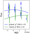 |
Fig. 2. Light curve of 2018cvq, shown at maximum light, along with the modeled SALT2 light curve, as well as χ2 relative to raw photometric uncertainties. 2018cvq was selected as the SN Ia in the sample with the largest number of epochs at maximum light, where evolution of the light curve is smallest. |
However an approach attributing outliers from light-curve fits to unbudgeted errors would potentially wash out exactly the light-curve features we want to examine in this work. In order to mitigate this issue as best as possible, we assumed that the photometry errors are uncorrelated in time, while physical light-curve features show correlation on a timescale of ∼5 days. We then fit light-curve residuals (relative to the SALT2 model with parameters published in the main data release) with a Gaussian process to determine the amplitude of each contribution.
We used the package celerite2 (Foreman-Mackey et al. 2017; Foreman-Mackey 2018) to fit the sample of light-curve data. For a given light curve in some band X, we define σX as the estimate of the relative unbudgeted, uncorrelated photometric error. We define the nuisance parameter σXCorr as the relative amplitude of correlated, potentially physical, light-curve variation in percentage units. We take the mean of the process to be the predicted flux of the fiducial SALT2 fit from the DR2 sample FX(p), where p is the phase of the observation, and the kernel of the Gaussian process has two components: (a) a diagonal, uncorrelated error floor equal to the sum in quadrature of the budgeted photometric error and σX in magnitude units, and (b) a Matérn 3/2 kernel with 5 day scale length and amplitude equal to σXCorr in magnitude units. The hyperparameters σXCorr and σX are taken to be shared across the ZTF sample. We made no K-corrections in this simple model of unbudgeted errors, assuming that the restricted redshift range of the ZTF sample mean that such effects are small in the residuals to the SALT2 model. With three bands, we have six parameters to determine. We fitted these Gaussian processes simultaneously across the whole sample, maximizing the log-likelihood of the fit with respect to the six parameters. Our fitted parameters are shown in Table 1, and an example light-curve fit is presented in Figure 3.
Estimated unbudgeted uncertainties in the ZTF photometric dataset.
 |
Fig. 3. Illustration of the Gaussian process inference described in Section 2.3 as applied to the light curve of 2019gvw. First panel: SALT2 fit to the light curve, along with observations (binned to 1 day resolution). Second panel: residuals of SALT2 fit. These residuals show both correlated behavior and uncorrelated noise. Third panel: Gaussian process, conditioned on observed residuals, with hyperparameters from Table 1, showing the possible correlated structure we ultimately hope to include in the trained SALT model. Fourth panel: leave-one-out residuals from Gaussian process, showing expected scatter and reduced correlation. |
We find that coherent variations in the residuals are detected in all 3 bands, particularly in i-band, confirming that there are likely variations in SN Ia light curves beyond those addressed by the SALT2 model. We also find significant uncorrelated errors at scales ∼1 − 2%.
Based on these results we added (in quadrature) an error floor to the estimated photometric uncertainties equal to σX ⋅ FX(p) to all photometry incorporated into the training data. However we note that leave-one-out testing of the Gaussian process fits finds 3σ outliers at rates approximately 5 times higher than predicted by this model (756 outliers vs 156 predicted), implying that our error floors may not capture non-Gaussian noise in the data. Further, the Gaussian process used here cannot correct distinguish time-correlated photometric errors (effects from correlation in seeing, bad subtractions, etc.) from variation in the true light curve. And as is detailed in Lacroix et al. (in prep.) the calibration of the ZTF data is ongoing work. As a result we are unable to conclude that our model presented in this work will be of quality sufficient for use in cosmological analysis, and cannot recommend use in that context until we have reached a better understanding of statistical and calibration uncertainties in the ZTF data. Future photometric releases are expected to use a scene-modeling pipeline, and are expected to greatly improve the consistency of uncertainty estimates.
3. SALT and SALTshaker
The SALTshaker code3, first presented in K21, was designed to allow the creation and training of SALT models in Python. Our primary goal in this work was to add an extra component. In order to extend the model with an additional component, as well as make future modification easier, we have refactored the code to use the JAX library, which compiles Python code to optimize performance and allow automatic differentiation of arbitrary functions via the chain rule (Bradbury et al. 2018). The SALTshaker code uses the derivatives of the likelihood function to guide the optimizer; previously, these derivatives were coded by hand. By relying on the autodiff functionality of the JAX library we can now allow the inclusion of arbitrary, user-defined functions for constraints, priors, and color laws without requiring a user to make multiple modifications across the program structure. As a result, the new code is more performant, modular, and expandable.
Concurrently the optimization process was simplified. The Gauss-Newton optimizer included in the original code has been retained, but a new optimizer using a gradient-descent method was used in this work. The original code alternated optimization of the flux and error model during the core fitting loop. Our revised optimizer uses a short burn-in period wherein the error model parameters are fixed while the flux model is fit before “turning on” the error model and fitting these parameters simultaneously. However we find that allowing the color scatter to be fit simultaneously with the rest of the model results in undesirable behavior due to the regularization prescriptions. Evaluation of the color scatter takes place after optimization has otherwise terminated, and only the color and color law parameters are allowed to be free during this step. Testing has shown that differences between the final surfaces trained with the new and old optimizer are present only at the level of mmag. The upgrades to the codebase have greatly improved the speed of the code from 1 day for a full training on the original K21 sample on a laptop, to ∼2 hours using the expanded sample with the revised code.
3.1. Model description
We here introduce SALT3+, a new model that extends the dimensionality of the SALT framework to model more complex light-curve features.
We model the flux of a SN Ia as a function of phase and wavelength
![Mathematical equation: $$ \begin{aligned} F(p,\lambda ) =&\mathrm{max}(0, x_0 [M_0(p,\lambda ;\boldsymbol{m}_{0}) + x_1 M_1(p,\lambda ;\boldsymbol{m}_{1})\nonumber \\&+ x_2 M_2(p,\lambda ;\boldsymbol{m}_{2})] \cdot \exp (-0.4 \cdot c \cdot \mathrm{CL}(\lambda ;\boldsymbol{cl}))), \end{aligned} $$](/articles/aa/full_html/2025/05/aa52578-24/aa52578-24-eq1.gif) (1)
(1)
where x0 represents the overall flux normalization, {x1, x2} model the intrinsic variation of the SNe Ia, and c a color parameter accounting for intrinsic and/or extrinsic dust reddening4. Flux surfaces {M0, M1, M2} are spectral energy distributions (SEDs) defined on a basis of two dimensional, third-order B-splines. CL(λ; cl) is a continuous piecewise function (with continuous first derivatives) defined as a polynomial between 2800 and 8000 Å, and linear in wavelengths outside of that range. The quantities {m0, m1, m2, cl} are parameters controlling these elements of the model, which are determined by the training code. In addition to including an additional component, we explicitly required the flux to be positive. The flux equation is integrated over each bandpass, to determine photometric fluxes. In the training, spectroscopic fluxes are further modified by a recalibration factor of  , where ai are polynomial coefficients, fitted for each spectrum. The NRecal., the number of spectral recalibration coefficients per spectrum are set as configuration options. This factor ensures that the calibration of the model is sourced from photometry, rather than spectra, while retaining spectral information about local features.
Diversity in the SN Ia population that is not described by the flux surfaces {M0, M1, M2} is accounted for by a two term variance model. The first is the “error model”, given as a function of phase and central filter wavelength for a given photometric band λc
![Mathematical equation: $$ \begin{aligned} {\Sigma }&= \begin{pmatrix} \sigma _{M_0,M_0}(p,\lambda _c)&\sigma _{M_0,M_1}(p,\lambda _c)&\sigma _{M_0,M_2}(p,\lambda _c)\\ \sigma _{M_0,M_1}(p,\lambda _c)&\sigma _{M_1,M_1}(p,\lambda _c)&\sigma _{M_1,M_2}(p,\lambda _c) \\ \sigma _{M_0,M_2}(p,\lambda _c)&\sigma _{M_1,M_2}(p,\lambda _c)&\sigma _{M_2,M_2}(p,\lambda _c) \end{pmatrix} \nonumber \\ {x}&= \begin{pmatrix} 1 \\ x_1 \\ x_2 \end{pmatrix} \nonumber \\ \sigma ^2_f(p,\lambda _c)&= \left[x_0 \exp (c \cdot \mathrm{CL}(\lambda _c))\right]^2 {x}^T {\Sigma }\ {x} \end{aligned} $$](/articles/aa/full_html/2025/05/aa52578-24/aa52578-24-eq3.gif) (2)
(2)
similarly to the SALT3 error model. Here, the error components σM, M are each zeroth order B-splines, whose parameters are determined during training. These represent additional variability associated with each parameter, allowing the model to assign different uncertainties to different SNe. The second component is the “color scatter” k(λc), a covariant uncertainty that allows light curves of the same SN in different bands to be coherently offset relative to one another. This component of the model is akin to chromatic models of intrinsic scatter like that of Guy et al. (2010) and the diagonal terms of the covariance matrix from Chotard et al. (2011). The color scatter and total covariance matrix are defined
![Mathematical equation: $$ \begin{aligned} k(\lambda ;\boldsymbol{a})&= \exp \left(\sum ^4_{i=0} \boldsymbol{a}_i \lambda ^i\right)\\ \left(\Sigma _{\mathrm{Model}}\right)_{ij}&= \delta _{ij} \sigma ^2_f\left(p_i,\lambda _{c (i)}\right)\nonumber \\&\quad + {\left\{ \begin{array}{ll} k^2\left([\lambda _c]\right) \left(\boldsymbol{f}_{\rm Model}\right)_i \left(\boldsymbol{f}_{\rm Model}\right)_j&X_i = X_j\\ 0&\mathrm{otherwise} \end{array}\right.} \end{aligned} $$](/articles/aa/full_html/2025/05/aa52578-24/aa52578-24-eq4.gif) (3)
(3)
where δij is the Kronecker delta, Xi is the photometric band in which the measurement was made, and (fModel)i is the predicted flux for a given data point. The parameters controlling the components, color law, error model, and color scatter are determined during the training process by a log-likelihood minimization evaluated across the photometric and spectroscopic data (see K21 for the definitions of the likelihood terms).
3.2. Model definitions and priors
As the model described above is (mostly) linear, the fluxes modelled are invariant under a set of linear transformations among components and coordinates. As an example, a transformation that increases the magnitude of the components M0, M1, M2 and decreases all x0 by the same factor does not modify the final fluxes. To eliminate these degeneracies, we are required to make choices to uniquely determine the model. Previously, these definitions were enforced by narrow priors during training, then exactly enforced by post-processing after optimization concluded. The new code allows us to enforce constraints exactly throughout the training, by transforming the parameters to satisfy the constraints at each likelihood evaluation, using JAX’s autodiff capabilities to differentiate through the transformation. Here we define the SALT3+ model to satisfy the conditions:
-
The rest-frame synthetic B-band flux of the M0 component at peak is fixed such that mBpeak = 10.5 when x0 = 1.
-
The rest-frame synthetic B-band flux of the M1 and M2 components at peak is defined to be 05.
-
The distributions of the light-curve parameters c, x1, and x2 over the training sample are defined to have 0 mean.
-
The distributions of x1 and x2 have standard deviation 1.
-
The distributions of x1, x2, and c have no correlation in the training sample.
-
The color law is defined such that CL(4300 Å) = 0 and CL(5430 Å) = −1, corresponding to central wavelengths for B and V bandpasses.
-
In post-processing after training is complete, the mutual information of the {x1, x2} distribution (as measured from a kernel-density estimator) is minimized by a rotation of the components and coordinates. We then label the component with larger RMS flux values as M1 and the corresponding coordinate x1, and the other pair as {M2, x2}. Lastly, the sign of both components is set such that they have positive B-band flux at 15 days.
The first 6 definitions are analogous to those made in SALT3, defining x0 to represent the inferred peak B-band flux, c to represent a B − V color difference independent of any behavior with time-evolution, and M0 to represent the SED of the mean SN Ia. The final definition is novel for SALT3+, although similar in concept to the fifth definition, and similar in principle to priors for variational autoencoders such as PARSNIP (Boone 2021). The goal of the definition is to, as much as possible, separate different phenomena into different parameters; this makes later analysis easier. We find that the resulting x1 parameter is strongly aligned with the previously derived SALT2/SALT3 x1. Our modeling is entirely empirical and does not incorporate any theoretical information.
In a departure from the approach employed with previous SALT models, we include priors on the parameters during the training process. These priors are standard normals on the parameters {x1, x2} as well as a normal distribution with mean 0 and standard deviation 0.2 on c. This approach was chosen because the second component M2 is smaller in magnitude than M1 and further is only significantly detectable at some points of the light curve. As a result, for many SNe in the sample it is under-constrained, and the use of priors in the parameters helps to reduce the impact of overfitting in the training sample. As a further precaution against overfitting in the data, the surfaces are regularized by the use of penalty terms in the training objective function proportional to the derivatives; we use all three methods of regularization described in K21.
3.3. Model configuration and early data
The SALT model requires the training code to specify configuration options including the phase and wavelength range over which the model will be defined, the resolution of the underlying model, and the degree of regularization. In addition to the inclusion of an additional spectral surface, other changes were made to the model configuration to ensure the model was well captured. The phase resolution of the underlying splines has been increased to 2.5 days from 3, while the wavelength resolution was kept identical to that of K21 at 69.3 Å, sufficient to cover broad SN features. All spectral recalibration polynomials were set to use a cubic polynomial for performance reasons, rather than setting the number of free parameters individually for each spectrum.
Ideally, the model’s phase coverage should begin immediately before the earliest SN explosions (relative to maximum light), with the {MX} components possessing no flux at that time and with the first derivatives zero. The third order B-splines can represent either an “expanding fireball” light curve with F ∝ t2 and/or deviations through the cubic component of the splines. Previous SALT models have used the phase range −20 days to +50 days. However, Miller et al. (2020) suggested, using early photometry of SNe Ia from the ZTF, that explosion may occur as much as 23 days prior to maximum light for some objects.
For SALTShaker, ZTF data gives greatly enhanced phase resolution, doubling the number of photometric epochs (not necessarily detections) available between −23 and −15 days. Thus, we examined whether the phase range needed to be expanded to better model the early-time evolution of the SNe Ia. In Fig. 4, we show early time photometric residuals relative to zero flux, roughly corresponding to detection significance. Only a small proportion of SNe can be individually detected at such early times, but in aggregate, we observe nonzero flux across the population as a whole. Visually, high x1 SNe are detected earlier compared to low x1 SNe, which can be undetectable even 15 days prior to maximum light.
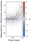 |
Fig. 4. Early time photometric fluxes, relative to photometric uncertainties, in the expanded training sample. Each point is a single photometric measurement, colored according to the x1 value of the supernova it belongs to. Crosses show mean values binned by both x1 and phase. Negative flux measurements are possible due to measurement uncertainties in difference imaging/scene modelling. Observations of SNe with x1 values close to the center of the distribution have been made partially transparent, to emphasize the edges of the population. PS1MD and Foundation data have been excluded from this plot, as some residuals showed indications of image subtraction issues. |
Running SALTShaker with the previously standard phase range of −20 to +50 days, we noted that the flux in M1 and M2 surface at −20 days did not typically converge to 0; furthermore, adding a constraint on the model that the initial flux and/or the first derivative of the flux be 0 led to visually different model light curves. Although no individual epochs are a detection at that early time, the aggregated weight of the entire sample is sufficient to affect the model. Running the model on this data with a minimum phase range of −23 days, we found that the resulting model, while showing small residuals at the edges of the phase range, does not predict any SNe to have observable (> 1σ) flux before −21 days. Therefore, our final model used the phase range −21 days to +50 days, to ensure the entire early evolution of the population is captured without adding unused flexibility to the model.
4. Results
4.1. Model surfaces
We first visualize the surfaces produced by the SALTshaker code, in order to describe the modeled behavior.
4.1.1. Synthetic light curves
As expected, adding a second component to the model is overall a relatively small effect. In Fig. 5, we show synthetic light curves over a range of parameter values. As can be seen, the size of the M2 component is much smaller than the M1 component. While M2 is empirically derived over the whole phase and wavelength range, and is not associated in principle with any particular physical effect, we can qualitatively describe the major impacts on model light curves. Increase in x2 implies a higher peak and faster decline in g-band (as contrasted to M1, which slows both the rise and decline times of the SN). In i band, x2 also increases the amplitude of the secondary maximum relative to the primary, while x1 shifts the time at which the secondary maximum peaks (see also Deckers et al. 2025). More extreme values of x2 create a visible “kink” in the i-band light curve in the primary peak. This feature was previously noted and discussed by Pessi et al. (2022), who found that the strength of the feature showed little correlation with light-curve stretch, in agreement with our results here. x2 is most measurable as a time-dependent effect in color curves, which are shown in Fig. 6. The contrast is most simply seen in r − i, where x1 is visible as a constant spread around a fixed slope, while x2 modifies the value of the slope.
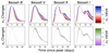 |
Fig. 5. Light curves for the SALT3+ model. Upper figure shows the variation in three bands as a function of x1 with x2 fixed to 0. Lower figure shows the variation as a function of x2 with x1 fixed to 0. Any other values will be represented by a linear combination of those light curves. |
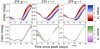 |
Fig. 6. Color curves for the SALT3+ model in magnitudes. Upper figure shows the variation in three bands as a function of x1 with x2 fixed to 0. Lower figure shows the variation as a function of x2 with x1 fixed to 0. Any other values will be represented by a linear combination of those light curves. |
4.1.2. Spectral effects
As SALT is a spectral model, besides examining light curves we also inspect the effect of parameter changes on model spectra. Particularly at maximum light, the model has an abundance of spectral data to constrain the underlying surfaces. The spectra as a function of phase, x1, and x2 are plotted in Fig. 7. To measure spectral features at maximum light, we used a fully automated and public code for spectral fitting, spextractor6 (Papadogiannakis 2019; Burrow et al. 2020). The code uses a nonparametric, Gaussian process (GP) regression to get the minima for the individual features. It is based on the python package GPy (GPy 2012) and uses a Matern 3/2 kernel for smoothing the spectra. In Fig. 8 we show how changes in x2 affect the width and velocity of spectral features in model spectra at maximum light in B-band, where most SN spectra are taken. In general we observe that increased x2 is associated with a higher line velocity, with a wavelength-dependent effect on pseudo-equivalent widths. The iron line at 4800 Å is the only one to reverse the sign of the velocity trend.
 |
Fig. 7. Synthetic spectra of SALT3+ across phase, x1, and x2. Left panel shows variation with x1, right panel shows variation with x2 from −5 days to +15 days. |
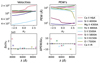 |
Fig. 8. Spectral effect of x2 at maximum light. Top left panel show velocity measured from spectral features as a function of x2, while top right panel shows pseudo-equivalent widths (PEW) as a function of x2. Bottom panels show slopes as a function of wavelength. |
Previous work has looked at the effect of spectral velocity on SN Ia light curves and/or Hubble residuals. Our results indicate a positive correlation between g − r/B − V color and spectral velocity of ∼0.04 mag, and a equivalently strong effect with opposite sign in redder (i.e. r − i) colors. Qualitatively, this is in agreement with previous work (Wang et al. 2009; Mandel et al. 2014; Dettman et al. 2021). However, we do not presently see evidence of a host-galaxy correlation with x2 (see Sect. 4.3.2), while some previous results have noted significant correlation between velocity and galaxy types (Wang et al. 2013; Pan et al. 2015; Pan 2020). Notably velocity associations with mass were also not seen previously with SALTshaker (Jones et al. 2023) or within the ZTF sample by Burgaz et al. (2025). However x2 likely does not capture all velocity variation in SN Ia, and/or improvements to the model may allow more precise measurements of host behavior.
4.1.3. Model uncertainties and color dispersion
The SALTshaker code, in addition to estimating the fluxes characterizing the SN Ia population, also estimates the unmodelled variation. This includes a component that is assumed to be stochastic, and will thus typically contribute little to the final error budgets. However a much more significant factor is the color dispersion, k(λc). This gives a relative, covariant uncertainty on each individual band in a light curve. As a consequence of the covariance, the color dispersion, for any given SALT model, sets a fundamental error floor on the parameters c and mB that cannot be reduced by additional epochs/more precise photometry, only additional filters. Further, the color dispersion is the only means provided to the model to account for phenomenology too complex to be included in the parametrization. As a result, the size of the color dispersion represents both a minimum statistical uncertainty, and an indicator of the size of potential systematic uncertainties in a given model.
Accounting for x2 results in a significant reduction in the color dispersion. We compare the color dispersion of SALT3.K21 and SALT2.T21 to SALT3+ in Fig. 9. The color dispersion is substantively lower for our version of the model across most wavelengths used in cosmological analysis, with the exception of the i band. In the rest frame V-band, color dispersions are reduced to the mmag level, well below typical photometric uncertainties. Consistently high color scatters in the i band may indicate difficulties with correctly fitting dust across all bands simultaneously with only a single color parameter. Studies such as Amanullah et al. (2015), Mandel et al. (2017), Brout & Scolnic (2021), Johansson et al. (2021), and Grayling et al. (2024) indicate that SN Ia colors are likely sourced from both extrinsic and intrinsic sources, that may contribute to differential wavelength dependence across the SN Ia population. Variance in dust population parameters such as RV from galaxy to galaxy may be a significant effect (cf. Popovic et al. 2023; Wojtak et al. 2023; Grayling et al. 2024). Preliminary cross-calibration studies (Dovekie, Popovic et al., in prep.) indicate an improved calibration solution for ZTF leads to a color scatter below that of SALT3.K21 in i band, although still a local maximum. Other causes of systematic uncertainty in the i-band may include internal calibration of different surveys, calcium features, or further physics beyond x2 associated with the second peak.
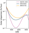 |
Fig. 9. Color dispersion, defined in terms of % uncertainty in the overall normalization of a given photometric band for a given supernova. Wavelength range shown here is the range of central filter wavelengths present in the training sample. |
4.2. Light-curve fitting
We fitted our model to light curves to the ZTF sample, as well as the K21 compilation. We applied less restrictive light-curve quality cuts more typical of cosmology analysis than required for the training sample.
-
At least one measurement in at least two bands after peak brightness (5 < p < 20), to constrain the shape and color.
-
At least one epoch between −20 < p < −1 to ensure a constraint on time of maximum.
-
At least six epochs in any bands between −10 < p < 35.
-
Classified as a normal SN Ia, or belonging to the 91T subtype.
We performed our light-curve fits using SNANA (Kessler et al. 2009b), which has been upgraded to allow multi-component SALT models to be fit. Our fits were maximum likelihood based, although we included unit normal priors centered at 0 on x1 and x2.
4.2.1. Parameter distributions
The shape of the parameter distributions could contain information about the underlying physics of the SN Ia populations. While the scale and location of the distribution are set by the model definitions (see Sect. 3.2) and are thus not informative, the other moments of the distribution may provide insight into underlying physics (see for example Ginolin et al. 2025a,b). We show the distribution of parameters x1, x2 fitted to the sample in Fig. 10. The shape of the x1 distribution is familiar relative to that found in other work (Ginolin et al. 2025b from the ZTF DR2; also Kessler & Scolnic 2017; Nicolas et al. 2021; Wojtak et al. 2023), showing a negative skew. The shape of the x2 distribution is far more Gaussian. Understanding the intrinsic shape of the x2 distribution however will require deconvolution with the noise, which forms a substantial portion of the observed distributions due to the high x2 uncertainties.
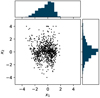 |
Fig. 10. Distribution in two dimensions of the x1, x2 parameter space for the ZTF sample using only SNe Ia within the volume-limited sample (z < 0.06). |
4.2.2. Parameter uncertainties
We show the estimated parameter uncertainties in Fig. 11 for each of the parameters. As discussed in Sect. 4.1.3, the color dispersion bounds from below the uncertainties in color and magnitude, resulting in very few objects with color uncertainties < 0.02 mag for SALT3.K21. The reduction in color dispersion effectively removes this floor, eliminating the sharp edge in the distribution. Magnitude and x1 uncertainties are reduced across the board. However, x2 is poorly constrained for most objects, and is dominated by the N(0, 1) prior.
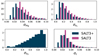 |
Fig. 11. Distribution of parameter uncertainties as calculated under each SALT3+ and SALT3.K21. |
We investigate some of the factors that contribute to an effective measurement of x2. Figs. 12 and 13 show that SNe observed with more filters reduce the correlation between x2 and c, and that uncertainty in x2 shows dependence on the total number of measured photometric epochs. In particular, at least three photometric filters are typically necessary to separate c from the x2 parameter to any significant degree.
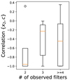 |
Fig. 12. Boxplot showing the distribution of reduced correlation between c and x2 uncertainties, grouped by the number of filters observed, among SNe from surveys other than ZTF. Correlation coefficient can range between −1 and +1. |
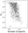 |
Fig. 13. Distribution of uncertainty in x2 as a function of the number of epochs in the fit. |
4.2.3. Comparison of SALT3.K21 and SALT3+
Changes in light-curve model affect ultimate cosmology results through changes to the fitted parameters. In Fig. 14 we show the difference in SALT3.K21 parameters relative to SALT3+ parameters, as a function of fitted x2. A linear trend in Δc is evident by eye and highly correlated, with Pearson r = −0.84, and a slope of 0.0251 ± 0.0006. The x1 difference Δx1 shows an effect of marginal significance, with a slope of 0.0062 ± 0.0025. We conclude that fits with SALT3.K21, ignorant of the x2 effect, attempt to compensate with the two ingredients available to the fitter, x1 and c. These trends indicate that while x2 is a significantly smaller effect than x1, and often has large uncertainties, fitting SNe Ia without including x2 in the fit will lead to significant changes in color parameters.
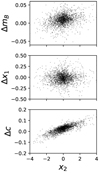 |
Fig. 14. Difference in fitted light-curve parameters between SALT3.K21 and SALT3+ as a function of fitted x2. |
4.3. Cosmology Implications
We created Hubble residuals using a simple linear standardization to allow comparison of cosmological performance between the previous SALT3.K21 model and the new SALT3+ model. In order to see the effect of the new model clearly, we cut the sample based on the fitted SALT3+ parameters with the following requirements:
-
The squared sum of x1 and x2 less than 9 (52 objects fail this cut).
-
c between −0.2 and 0.4 mag (30 objects fail).
-
Estimated uncertainty in c less than 0.1 mag (19 objects fail).
-
Estimated uncertainty in x1 less than 0.5 (205 objects fail).
-
P-value of fit greater than 1e-5 (185 objects fail).
-
Reduced correlation of x2 and c less than 0.9 (727 objects fail).
Overall, of 2214 objects successfully fit by SNANA, 1161 (52%) passed these cuts, of which the last cut is the most significant. For many objects, SNANA reports parameter uncertainties that indicate that the fitter is unable to constrain x2 and c independently. Many of these objects have been observed in only two filters; as x2 is most significantly constrained by the effect on color-curves, this is problematic. In order to clearly see the effect of the introduction of x2 on the cosmological nuisance parameters, we remove these SNe. Of the objects that pass other cuts, 120 do not have masses available from either Pantheon+ or the ZTF DR2; for these, we include them in the fit and apply no mass step. Although we fit and validate on (mostly) overlapping samples, the Tripp estimator plays no role in the SALTshaker, and performance on these metrics is not evaluated in training.
Given a SN at redshift z in the CMB rest frame with fitted parameters x0, x1, x2, c, associated covariance matrix Σ, and host galaxy stellar mass M, the Hubble residual Δμ is defined by analogue to the Tripp estimator (Tripp 1998)
 (4)
(4)
where μ(z) is the distance modulus calculated under flat ΛCDM with Planck Collaboration VI (2020) cosmological parameters. Corresponding Gaussian uncertainties are estimated as
 (5)
(5)
where σμ, z is computed from a peculiar velocity uncertainty of 250 km s−1 using the derivatives of the distance modulus with redshift, and σlens = 0.055z (Jönsson et al. 2010).
These Hubble residuals depend on nuisance parameters: ℳ the overall normalization, intrinsic standardization coefficients αX, color standardization coefficient β (roughly analogous to an “average” RB across the sample if colors are assumed to be dust reddening), “mass step” γ, and the unparameterized or “intrinsic” scatter in the Hubble diagram σint. We also find that the ZTF sample shows much higher intrinsic scatter than the data from the K21 compilation, so we allowed the intrinsic scatter for ZTF to be independent of the intrinsic scatter of the other data. We computed these parameters for our sample by maximizing a Gaussian log-likelihood ℒ = −∑log(σμ)/2 + (Δμ/σμ)2/2, using light-curve fits made with both the new model and the most recent version of SALT3.K21 (setting α2 = 0 in the latter case). As an optimizer, we use Minuit (James & Roos 1975), and report the parameter error estimates from the Hessian matrix derived. This simple approach does not correct for regression or selection biases, but allowed us to demonstrate some of the differences between SALT3+ and SALT3.K21. We present the fitted nuisance parameters and likelihoods in Table 2.
Tripp nuisance parameters and maximum likelihood, compared between SALT3+ and SALT3.K21.
The Tripp fits show significant evidence in favor of the higher dimensionality; the log-likelihood difference across the full sample of corresponds to a ΔAIC = 66.4, favoring SALT3+ at ∼8.3σ with the inclusion of a single extra parameter in the fit. Likelihood ratios favor SALT3+ in both ZTF and non-ZTF subsamples. RMS scatter in the data slightly decreases with the additional parameter, from 0.184 to 0.178 mag. ℳ differences between the models are not in general physically relevant, as the zero-point of the model is arbitrary, varying with mean properties of the training sample. Further, a blinding factor has been added to ℳ for the ZTF sample, as discussed in Rigault et al. (2025b). However we note that when splitting the data between ZTF and non-ZTF subsamples, significant differences are present in α2, γ, and β, that may indicate issues of generalizability from ZTF to other surveys. These may simply be indications of the different selection functions between surveys, or reflect the current incompleteness of the ZTF calibration solution. Additionally, while the extended model is preferred by both samples, the significance outside of ZTF is only ∼2.5σ.
Comparing the residuals between the models, the Hubble residuals made using the SALT3.K21 model show a trend in x2 of ∼0.05 mag that can be seen in Fig. 15. The effect is primarily driven by the strong effect in the color parameter c seen in Fig. 14, with a small countervailing effect in x1. If x2 vary across populations, this could potentially lead to a systematic of the same magnitude in one-dimensional SALT-based analyses. We examine our sample to see whether there is any evident trend of x2 with redshift; for now, we do not see any apparent significant effect. Taking the difference in mean x2 at z < 0.15 and z > 0.15, we find Δx2 = 0.054 ± 0.036, implying a potential systematic of 2.1 ± 1.5 mmag. This systematic may increase under alternate prior assumptions; a full analysis would require a complete population model (further discussed in Sect. 5).
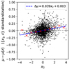 |
Fig. 15. Hubble residuals calculated using SALT3.K21, with standardization in x1 and c, against x2 calculated using SALT3+. Red crosses show binned residuals, with line of best-fit in blue. |
Interpreting differences in α between models is somewhat difficult. As the scales of xi are anchored by definition 4 in Sect. 3.2 to the demographics of the training sample, α changes between models may reflect empirical differences or mere demographic changes in the model from including ZTF in the training sample. To determine which effect is driving the lowered α1 seen in SALT3+, we need to anchor α1 to a specific light-curve feature. We use Δm15(B) since it was the first feature of the stretch effect discovered. Using synthetic light curves, we evaluate ∂Δm15(B)/∂x1 for both models at {z = 0, c = 0, x1 = 0, x2 = 0}, then calculate  for both models; since the quantities present on the L.H.S. are light-curve features independent of sample demographics, this slope should be comparable between models (see also discussion in Grayling et al. 2024). We find
  to be 0.796 for SALT3 and 0.593 for SALT3+. This implies that the decrease in α1 seems to be a real difference between models, rather than a purely demographic difference. This may reflect increased scatter in measured x1 values due to the additional degree of freedom in the fit. However, the increase in β nevertheless allows SALT3+ to explain more scatter than the SALT3.K21 model.
4.3.1. Colors
As c is defined by reference to a fixed quantity (that is, B − V color), differences from model to model in β across the same sample are more likely to be physically relevant. To evaluate the significance of the effect, we bootstrap resampled the SNe and refit the Tripp estimator for both SALT3+ and SALT3.K21 with the resampled data. We estimate the difference between β as 0.22 ± 0.03. The increase in β seen between SALT3 and SALT3+ is likely here to be driven by increased accuracy in color measurements, bringing β somewhat closer to RV values typically inferred from SED fitting of galaxy populations (e.g. Salim et al. 2018; Duarte et al. 2025; Murakami et al. 2025). We note a difference in β between ZTF and non-ZTF samples, which is stronger in the new model. This may be due to different dust demographics in the more complete sample of ZTF than previous data, explored in more detail in Ginolin et al. (2025a) and Popovic et al. (2025).
We next studied the distribution of the color parameter. A standard approach in the field, also used in Ginolin et al. (2025a), is to assume that host galaxy dust shows an exponential distribution in optical depth τ, while intrinsic color is normally distributed with mean μ and scatter σc, int. We used the ZTF supernovae to derive intrinsic distributions, assuming that the sample is volume limited below z < 0.06. With fitted color parameter c and associated uncertainty σc, the likelihood over the color distribution is
 (6)
(6)
using E(μ, σ, τ) to denote the convolution of the PDFs of the exponential and normal distributions. We maximized this likelihood function over the 358 ZTF SNe passing all light-curve cuts, besides the cut on color, below z < 0.06 and report the values of the derived population parameters in Table 3. The SALT3+ colors show a narrower distribution in both σc, int and τ, with the latter difference proving more robust in bootstrap testing. The narrower distribution is consistent with the x2 component accounting for a fraction of the observed color distribution. We show the derived intrinsic distributions and observed distributions in Fig. 16.
Intrinsic color distribution parameters, compared between SALT3 and SALT3+.
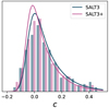 |
Fig. 16. Observed and inferred intrinsic color distributions derived from the volume-limited ZTF sample. Solid lines show the convolved exponential distribution with parameters from Table 3. Histograms show the observed distribution, which are consistent with the inferred intrinsic distributions widened by noise. |
In Fig. 17, we show the stretch-corrected, but not color-corrected, Hubble residuals. Previous analyses posited that red and blue SNe may obey different color laws (see e.g. Mandel et al. 2017); current cosmology analyses such as Brout et al. (2022a) as well as Rubin et al. (2023) have explicitly or implicitly used a nonlinear color correction. This has been physically justified by appeal to distinct color-luminosity relations for host galaxy reddening in the red tail of the color distribution and intrinsic color in the blue tail. Here we note that the nonlinearity of the luminosity-color relation appears increased by the new model. To investigate further, we redefined the Tripp relation by setting β in Equation (6) to β = β0 + β′⋅c. Fitting the sample, a quadratic fit to the data is favored with either model, with a likelihood ratio of Δℒ = 24.9 for the full sample. With a single additional parameter, this corresponds to ΔAIC = 47.8. We then evaluated the difference in β′ between models by bootstrap resampling, finding Δβ′ = 0.35 ± 0.16, at ∼2.1σ significance. This is consistent with an interpretation that the inclusion of x2 in the fit improves the precision of c as a tracer of host-galaxy extinction. Nonlinearity can also reflect regression dilution with an asymmetric underlying c distribution (see the appendix of Ginolin et al. 2025a). The increased nonlinearity could be driven by reduced color uncertainties producing a c distribution more strongly dominated by the (asymmetric) exponential tail. Ginolin et al. (2025a) did not find strong evidence of an intrinsically nonlinear color relation in the ZTF sample using SALT2.T21-derived colors.
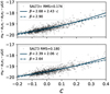 |
Fig. 17. Absolute magnitudes, corrected for x1 and x2 but not color, as compared between models. Upper panel shows residuals calculated with SALT3+, in lower panel with SALT3. Solid line shows a quadratic fit to the data, dashed line shows a linear fit. |
4.3.2. Host properties
We did not find any effective correlation between host galaxy properties and x2. Likely, the significant noise present obscures any relation present. We show the distribution, split by host galaxy mass at 1010 M⊙, in Fig. 18. The mass step seems somewhat smaller in the ZTF sample, however this does not generalize to the non-ZTF sample.
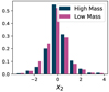 |
Fig. 18. x2 distribution, split between high and low mass galaxies at 1010 M⊙. |
5. Conclusions
We present SALT3+, a new SALT model with an additional principal component. Although preliminary, the model trained here has been added to both the sncosmo (Barbary et al. 2015, 2016) and SNANA (Kessler et al. 2009b) codes for use in light-curve fitting. The new model shows particular improvement in producing informative colors for cosmology analysis.
However, the model as presented here is not ready for use in a full cosmology analysis. Our work here should thus be regarded as exploratory. The ZTF calibration is still a work in progress, with calibration uncertainties greater than centimag level. Accounting for these corrections can be forecasted to improve the uncertainties in the model (particularly i band), and improve generalization from ZTF to non-ZTF surveys. Further, we note that the issues seen with uncertainties in Sect. 2.3 and the additional intrinsic scatter in Sect. 4.3 may also affect the light-curve model. Future data releases from the ZTF collaboration plan to use scene-modelled photometry, discussed in Lacroix et al. (in prep.). The Hubble residuals we presented have not been corrected for selection bias or regression dilution. The results on standardization presented here should thus be regarded as preliminary. Correctly accounting for these biases requires either frequentist forward-simulation, or a Bayesian hierarchical model. Frequentist analysis requires the derivation of parent populations suitable for use in a BBC-based analysis (Kessler & Scolnic 2017) through use of a code such as Dust2Dust (Popovic et al. 2023). Bayesian approaches include codes like UNITY (Rubin et al. 2015, 2023), STEVE (Hinton et al. 2019), BAHAMAS (March et al. 2011; Shariff et al. 2016; Rahman et al. 2022), and others (e.g. Mandel et al. 2017; Feeney et al. 2018; Wojtak et al. 2023) that can simultaneously derive cosmology and population parameters. Either approach will require further work.
Possible physical origins of the effects we describe here are unclear. Spectral features indicating a velocity trend along with changes in broadband colors may reflect a different conversion of energy into thermal/kinetic components. Variation in velocity could indicate variation in the observed angle of an asymmetric explosion. The significant changes in calcium features in our synthetic spectra could be a result of calcium plumes in the ejecta (Khokhlov 1995; Pessi et al. 2022). Future work could investigate possible driving physics of these features.
As x2 affects the rising light curve less, our results support the conclusions of Hayden et al. (2019) that the most informative stretch information in the light curves is in the rise of the SN. We also conclude that SNe Ia must be observed in no fewer than three filters to robustly measure host galaxy extinction. Both of these emphasize the value of the ZTF data set in future cosmology. Further, evaluation of survey cadence strategies should likely incorporate these considerations. In addition, neglecting the second component in light-curve fits leads to a residual trend of 0.039 ± 0.005 mag in Hubble residuals; if there is demographic evolution in the second component, it could represent a systematic. However, we see no evidence for a shift in the mean of the x2 distribution with redshift, leading to an estimated systematic of 2.1 mmag ± 1.5 mag. We conclude that any systematics from optical light-curve features of higher order are likely to be less than this value, and that models of dimensionality higher than this are unlikely to be a requirement. However, estimates of systematic uncertainties from forward simulation techniques such as BBC are sensitive to the model used for simulating data. Extended light-curve models may be important for these purposes. As x2 shows little correlation with Hubble residuals as long as the phenomenology is included in light-curve fits, it may be unnecessary to explicitly parametrize the phenomenon for use in cosmology analysis. The Gaussian process model for light-curve residuals used by BayeSN (Mandel et al. 2022; Grayling et al. 2024) marginalizes over the light-curve variability, likely preventing an x2 effect from affecting their parameters as seen in Fig. 14. If accounting for x2 at the level of cosmological analysis is unnecessary, developing a more robust error model for a one-dimensional SALT model may be a promising direction for future work.
When inferring spectra from photometry (a convolved SED), narrow oscillations in the reconstruction are a common issue due to the lack of spectral resolution. This phenomenon is known as deconvolution noise.
These calibration solutions were also used by Taylor et al. (2023) to retrain SALT3.
Available at https://github.com/djones1040/SALTShaker
There is an error in Eq. (1) of K21, which neglected the factor of −0.4 in the exponential term.
By making this definition, the effects of x1 and x2 on the B-band maximum are absorbed into Tripp standardization parameters α1, α2.
Code is publicly available at github.com/astrobarn/spextractor
Acknowledgments
The authors thank Daniel Kasen for useful discussion. Based on observations obtained with the Samuel Oschin Telescope 48-inch and the 60-inch Telescope at the Palomar Observatory as part of the Zwicky Transient Facility project. ZTF is supported by the National Science Foundation under Grant No. AST-1440341 and a collaboration including Caltech, IPAC, the Weizmann Institute of Science, the Oskar Klein Center at Stockholm University, the University of Maryland, the University of Washington, Deutsches Elektronen-Synchrotron and Humboldt University, Los Alamos National Laboratories, the TANGO Consortium of Taiwan, the University of Wisconsin at Milwaukee, and Lawrence Berkeley National Laboratories. Operations are conducted by COO, IPAC, and UW. SED Machine is based upon work supported by the National Science Foundation under Grant No. 1106171 This work has been enabled by support from the research project grant ‘Understanding the Dynamic Universe’ funded by the Knut and Alice Wallenberg Foundation under Dnr KAW 2018.0067. AG acknowledges support from the Swedish Research Council, project 2020-03444. ST was supported by funding from the European Research Council (ERC) under the European Union’s Horizon 2020 research and innovation programmes (grant agreement no. 101018897 CosmicExplorer). T.E.M.B. acknowledges financial support from the Spanish Ministerio de Ciencia e Innovación (MCIN), the Agencia Estatal de Investigación (AEI) 10.13039/501100011033, and the European Union Next Generation EU/PRTR funds under the 2021 Juan de la Cierva program FJC2021-047124-I and the PID2020-115253GA-I00 HOSTFLOWS project, from Centro Superior de Investigaciones Científicas (CSIC) under the PIE project 20215AT016, and the program Unidad de Excelencia María de Maeztu CEX2020-001058-M. JHT is supported by the H2020 European Research Council grant no. 758638. L.G. acknowledges financial support from AGAUR, CSIC, MCIN and AEI 10.13039/501100011033 under projects PID2020-115253GA-I00, PIE 20215AT016, CEX2020-001058-M, and 2021-SGR-01270. UB is supported by the H2020 European Research Council grant no. 758638 We acknowledge the University of Chicago’s Research Computing Center for their support of this work. This project has received funding from the European Research Council (ERC) under the European Union’s Horizon 2020 research and innovation programme (grant agreement n°759194 – USNAC). GD is supported by the H2020 European Research Council grant no. 758638. This project has received funding from the European Research Council (ERC) under the European Union’s Horizon 2020 research and innovation programme (grant agreement n°759194 – USNAC). KM is supported by the H2020 European Research Council grant no. 758638. PN acknowledges support from the DOE under grant DE-AC02-05CH11231, Analytical Modeling for Extreme-Scale Computing Environments. Y.-L.K. has received funding from the Science and Technology Facilities Council [grant number ST/V000713/1].
References
- Abbott, T. M. C., Allam, S., Andersen, P., et al. 2019, ApJ, 872, L30 [Google Scholar]
- Aldering, G., Adam, G., Antilogus, P., et al. 2002, SPIE Conf. Ser., 4836, 61 [Google Scholar]
- Amanullah, R., Johansson, J., Goobar, A., et al. 2015, MNRAS, 453, 3300 [Google Scholar]
- Astier, P., Guy, J., Regnault, N., et al. 2006, A&A, 447, 31 [NASA ADS] [CrossRef] [EDP Sciences] [Google Scholar]
- Balland, C., Cellier-Holzem, F., Lidman, C., et al. 2018, A&A, 614, A134 [NASA ADS] [CrossRef] [EDP Sciences] [Google Scholar]
- Barbary, K., Rodney, S., Sofiatti, C., et al. 2015, https://doi.org/10.5281/zenodo.592747 [Google Scholar]
- Barbary, K., Barclay, T., Biswas, R., et al. 2016, Astrophysics Source Code Library [record ascl:1611.017] [Google Scholar]
- Bellm, E. C., Kulkarni, S. R., Graham, M. J., et al. 2019, PASP, 131, 018002 [Google Scholar]
- Betoule, M., Kessler, R., Guy, J., et al. 2014, A&A, 568, A22 [NASA ADS] [CrossRef] [EDP Sciences] [Google Scholar]
- Blagorodnova, N., Neill, J. D., Walters, R., et al. 2018, PASP, 130, 035003 [Google Scholar]
- Boone, K. 2021, AJ, 162, 275 [NASA ADS] [CrossRef] [Google Scholar]
- Bradbury, J., Frostig, R., Hawkins, P., et al. 2018, JAX: Composable Transformations of Python+NumPy Programs, http://github.com/google/jax [Google Scholar]
- Brout, D., & Scolnic, D. 2021, ApJ, 909, 26 [NASA ADS] [CrossRef] [Google Scholar]
- Brout, D., Scolnic, D., Popovic, B., et al. 2022a, ApJ, 938, 110 [NASA ADS] [CrossRef] [Google Scholar]
- Brout, D., Taylor, G., Scolnic, D., et al. 2022b, ApJ, 938, 111 [NASA ADS] [CrossRef] [Google Scholar]
- Burgaz, U., Maguire, K., Dimitriadis, G., et al. 2025, A&A, 694, A13 (ZTF DR2 SI) [NASA ADS] [CrossRef] [EDP Sciences] [Google Scholar]
- Burns, C. R., Stritzinger, M., Phillips, M. M., et al. 2014, ApJ, 789, 32 [Google Scholar]
- Burns, C. R., Parent, E., Phillips, M. M., et al. 2018, ApJ, 869, 56 [Google Scholar]
- Burrow, A., Baron, E., Ashall, C., et al. 2020, ApJ, 901, 154 [NASA ADS] [CrossRef] [Google Scholar]
- Chotard, N., Gangler, E., Aldering, G., et al. 2011, A&A, 529, L4 [NASA ADS] [CrossRef] [EDP Sciences] [Google Scholar]
- Dai, M., Jones, D. O., Kenworthy, W. D., et al. 2023, ApJS, 267, 1 [Google Scholar]
- Deckers, M., Maguire, K., Shingles, L., et al. 2025, A&A, 694, A12 (ZTF DR2 SI) [NASA ADS] [CrossRef] [EDP Sciences] [Google Scholar]
- Dekany, R., Smith, R. M., Riddle, R., et al. 2020, PASP, 132, 038001 [NASA ADS] [CrossRef] [Google Scholar]
- Dettman, K. G., Jha, S. W., Dai, M., et al. 2021, ApJ, 923, 267 [NASA ADS] [CrossRef] [Google Scholar]
- Duarte, J., González-Gaitán, S., Mourão, A., et al. 2025, A&A, submitted [arXiv:2503.04906] [Google Scholar]
- Feeney, S. M., Mortlock, D. J., & Dalmasso, N. 2018, MNRAS, 476, 3861 [NASA ADS] [CrossRef] [Google Scholar]
- Fernández, A., García, S., Galar, M., et al. 2018, Dimensionality Reduction for Imbalanced Learning (Cham: Springer International Publishing), 227 [Google Scholar]
- Foley, R. J., Scolnic, D., Rest, A., et al. 2018, MNRAS, 475, 193 [Google Scholar]
- Foreman-Mackey, D. 2018, RNAAS, 2, 31 [NASA ADS] [Google Scholar]
- Foreman-Mackey, D., Agol, E., Ambikasaran, S., & Angus, R. 2017, AJ, 154, 220 [Google Scholar]
- Fremling, C., Miller, A. A., Sharma, Y., et al. 2020, ApJ, 895, 32 [NASA ADS] [CrossRef] [Google Scholar]
- Ginolin, M., Rigault, M., Copin, Y., et al. 2025a, A&A, 694, A4 (ZTF DR2 SI) [NASA ADS] [CrossRef] [EDP Sciences] [Google Scholar]
- Ginolin, M., Rigault, M., Smith, M., et al. 2025b, A&A, 695, A140 (ZTF DR2 SI) [NASA ADS] [CrossRef] [EDP Sciences] [Google Scholar]
- GPy 2012, GPy: A Gaussian Process Framework in Python, http://github.com/SheffieldML/GPy [Google Scholar]
- Graham, M. J., Kulkarni, S. R., Bellm, E. C., et al. 2019, PASP, 131, 078001 [Google Scholar]
- Grayling, M., Thorp, S., Mandel, K. S., et al. 2024, MNRAS, 531, 953 [NASA ADS] [CrossRef] [Google Scholar]
- Guy, J., Astier, P., Nobili, S., Regnault, N., & Pain, R. 2005, A&A, 443, 781 [NASA ADS] [CrossRef] [EDP Sciences] [Google Scholar]
- Guy, J., Astier, P., Baumont, S., et al. 2007, A&A, 466, 11 [NASA ADS] [CrossRef] [EDP Sciences] [Google Scholar]
- Guy, J., Sullivan, M., Conley, A., et al. 2010, A&A, 523, A7 [NASA ADS] [CrossRef] [EDP Sciences] [Google Scholar]
- Hamuy, M., Phillips, M. M., Suntzeff, N. B., et al. 1996, AJ, 112, 2408 [Google Scholar]
- Hayden, B., Rubin, D., & Strovink, M. 2019, ApJ, 871, 219 [NASA ADS] [CrossRef] [Google Scholar]
- Hicken, M., Challis, P., Jha, S., et al. 2009, ApJ, 700, 331 [Google Scholar]
- Hicken, M., Challis, P., Kirshner, R. P., et al. 2012, ApJS, 200, 12 [Google Scholar]
- Hinton, S. R., Davis, T. M., Kim, A. G., et al. 2019, ApJ, 876, 15 [Google Scholar]
- Holtzman, J. A., Marriner, J., Kessler, R., et al. 2008, AJ, 136, 2306 [NASA ADS] [CrossRef] [Google Scholar]
- Hounsell, R., Scolnic, D., Foley, R. J., et al. 2018, ApJ, 867, 23 [NASA ADS] [CrossRef] [Google Scholar]
- James, F., & Roos, M. 1975, Comput. Phys. Commun., 10, 343 [Google Scholar]
- Jha, S., Kirshner, R. P., Challis, P., et al. 2006, AJ, 131, 527 [Google Scholar]
- Jha, S., Riess, A. G., & Kirshner, R. P. 2007, ApJ, 659, 122 [NASA ADS] [CrossRef] [Google Scholar]
- Johansson, J., Cenko, S. B., Fox, O. D., et al. 2021, ApJ, 923, 237 [NASA ADS] [CrossRef] [Google Scholar]
- Jones, D. O., Scolnic, D. M., Foley, R. J., et al. 2019, ApJ, 881, 19 [Google Scholar]
- Jones, D. O., Kenworthy, W. D., Dai, M., et al. 2023, ApJ, 951, 22 [NASA ADS] [CrossRef] [Google Scholar]
- Jönsson, J., Sullivan, M., Hook, I., et al. 2010, MNRAS, 405, 535 [NASA ADS] [Google Scholar]
- Kasen, D., & Woosley, S. E. 2007, ApJ, 656, 661 [NASA ADS] [CrossRef] [Google Scholar]
- Kenworthy, W. D., Jones, D. O., Dai, M., et al. 2021, ApJ, 923, 265 [NASA ADS] [CrossRef] [Google Scholar]
- Kessler, R., & Scolnic, D. 2017, ApJ, 836, 56 [Google Scholar]
- Kessler, R., Becker, A. C., Cinabro, D., et al. 2009a, ApJS, 185, 32 [Google Scholar]
- Kessler, R., Bernstein, J. P., Cinabro, D., et al. 2009b, PASP, 121, 1028 [Google Scholar]
- Khokhlov, A. M. 1995, ApJ, 449, 695 [Google Scholar]
- Kim, Y. L., Rigault, M., Neill, J. D., et al. 2022, PASP, 134, 024505 [NASA ADS] [CrossRef] [Google Scholar]
- Krisciunas, K., Bastola, D., Espinoza, J., et al. 2013, AJ, 145, 11 [Google Scholar]
- Krisciunas, K., Contreras, C., Burns, C. R., et al. 2017, AJ, 154, 211 [NASA ADS] [CrossRef] [Google Scholar]
- Kunz, M., Bassett, B. A., & Hlozek, R. A. 2007, Phys. Rev. D, 75, 103508 [Google Scholar]
- Léget, P. F., Gangler, E., Mondon, F., et al. 2020, A&A, 636, A46 [NASA ADS] [CrossRef] [EDP Sciences] [Google Scholar]
- LSST Dark Energy Science Collaboration (Mandelbaum, R., et al.) 2018, ArXiv e-prints [arXiv:1809.01669] [Google Scholar]
- Mandel, K. S., Narayan, G., & Kirshner, R. P. 2011, ApJ, 731, 120 [CrossRef] [Google Scholar]
- Mandel, K. S., Foley, R. J., & Kirshner, R. P. 2014, ApJ, 797, 75 [Google Scholar]
- Mandel, K. S., Scolnic, D. M., Shariff, H., Foley, R. J., & Kirshner, R. P. 2017, ApJ, 842, 93 [NASA ADS] [CrossRef] [Google Scholar]
- Mandel, K. S., Thorp, S., Narayan, G., Friedman, A. S., & Avelino, A. 2022, MNRAS, 510, 3939 [NASA ADS] [CrossRef] [Google Scholar]
- March, M. C., Trotta, R., Berkes, P., Starkman, G. D., & Vaudrevange, P. M. 2011, MNRAS, 418, 2308 [Google Scholar]
- Masci, F. J., Laher, R. R., Rusholme, B., et al. 2019, PASP, 131, 018003 [Google Scholar]
- Miller, A. A., Yao, Y., Bulla, M., et al. 2020, ApJ, 902, 47 [NASA ADS] [CrossRef] [Google Scholar]
- Murakami, Y. S., Riess, A. G., Ferguson, H. C., et al. 2025, ApJ, submitted [arXiv:2503.09702] [Google Scholar]
- Nicolas, N., Rigault, M., Copin, Y., et al. 2021, A&A, 649, A74 [NASA ADS] [CrossRef] [EDP Sciences] [Google Scholar]
- Pan, Y.-C. 2020, ApJ, 895, L5 [NASA ADS] [CrossRef] [Google Scholar]
- Pan, Y. C., Sullivan, M., Maguire, K., et al. 2015, MNRAS, 446, 354 [NASA ADS] [CrossRef] [Google Scholar]
- Papadogiannakis, S. 2019, Ph.D. Thesis, Stockholm University, Sweden [Google Scholar]
- Perley, D. A., Fremling, C., Sollerman, J., et al. 2020, ApJ, 904, 35 [NASA ADS] [CrossRef] [Google Scholar]
- Pessi, P. J., Hsiao, E. Y., Folatelli, G., et al. 2022, MNRAS, 510, 4929 [NASA ADS] [CrossRef] [Google Scholar]
- Phillips, M. M. 1993, ApJ, 413, L105 [Google Scholar]
- Planck Collaboration VI. 2020, A&A, 641, A6 [NASA ADS] [CrossRef] [EDP Sciences] [Google Scholar]
- Popovic, B., Brout, D., Kessler, R., & Scolnic, D. 2023, ApJ, 945, 84 [NASA ADS] [CrossRef] [Google Scholar]
- Popovic, B., Rigault, M., Smith, M., et al. 2025, A&A, 694, A5 (ZTF DR2 SI) [NASA ADS] [CrossRef] [EDP Sciences] [Google Scholar]
- Rahman, W., Trotta, R., Boruah, S. S., Hudson, M. J., & van Dyk, D. A. 2022, MNRAS, 514, 139 [NASA ADS] [CrossRef] [Google Scholar]
- Rest, A., Scolnic, D., Foley, R. J., et al. 2014, ApJ, 795, 44 [Google Scholar]
- Riess, A. G., Kirshner, R. P., Schmidt, B. P., et al. 1999, AJ, 117, 707 [Google Scholar]
- Rigault, M., Neill, J. D., Blagorodnova, N., et al. 2019, A&A, 627, A115 [NASA ADS] [CrossRef] [EDP Sciences] [Google Scholar]
- Rigault, M., Smith, M., Regnault, N., et al. 2025a, A&A, 694, A2 (ZTF DR2 SI) [NASA ADS] [CrossRef] [EDP Sciences] [Google Scholar]
- Rigault, M., Smith, M., Goobar, A., et al. 2025b, A&A, 694, A1 (ZTF DR2 SI) [NASA ADS] [CrossRef] [EDP Sciences] [Google Scholar]
- Rose, B. M., Dixon, S., Rubin, D., et al. 2020, ApJ, 890, 60 [NASA ADS] [CrossRef] [Google Scholar]
- Rubin, D. 2020, ApJ, 897, 40 [Google Scholar]
- Rubin, D., Aldering, G., Barbary, K., et al. 2015, ApJ, 813, 137 [Google Scholar]
- Rubin, D., Aldering, G., Betoule, M., et al. 2023, ArXiv e-prints [arXiv:2311.12098] [Google Scholar]
- Sako, M., Bassett, B., Becker, A. C., et al. 2018, PASP, 130, 064002 [NASA ADS] [CrossRef] [Google Scholar]
- Salim, S., Boquien, M., & Lee, J. C. 2018, ApJ, 859, 11 [Google Scholar]
- Saunders, C., Aldering, G., Antilogus, P., et al. 2018, ApJ, 869, 167 [NASA ADS] [CrossRef] [Google Scholar]
- Scolnic, D. M., Jones, D. O., Rest, A., et al. 2018, ApJ, 859, 101 [NASA ADS] [CrossRef] [Google Scholar]
- Shariff, H., Jiao, X., Trotta, R., & van Dyk, D. A. 2016, ApJ, 827, 1 [NASA ADS] [CrossRef] [Google Scholar]
- Siebert, M. R., Foley, R. J., Jones, D. O., et al. 2019, MNRAS, 486, 5785 [CrossRef] [Google Scholar]
- Taylor, G., Lidman, C., Tucker, B. E., et al. 2021, MNRAS, 504, 4111 [NASA ADS] [CrossRef] [Google Scholar]
- Taylor, G., Jones, D. O., Popovic, B., et al. 2023, MNRAS, 520, 5209 [NASA ADS] [CrossRef] [Google Scholar]
- Taylor, G., Lidman, C., Popovic, B., & Abbot, H. J. 2024, MNRAS, 528, 4643 [Google Scholar]
- Thorp, S., Mandel, K. S., Jones, D. O., Ward, S. M., & Narayan, G. 2021, MNRAS, 508, 4310 [NASA ADS] [CrossRef] [Google Scholar]
- Tripp, R. 1998, A&A, 331, 815 [NASA ADS] [Google Scholar]
- Vincenzi, M., Brout, D., Armstrong, P., et al. 2024, ApJ, 975, 86 [NASA ADS] [CrossRef] [Google Scholar]
- Walker, E. S., Hook, I. M., Sullivan, M., et al. 2011, MNRAS, 410, 1262 [NASA ADS] [CrossRef] [Google Scholar]
- Wang, X., Filippenko, A. V., Ganeshalingam, M., et al. 2009, ApJ, 699, L139 [NASA ADS] [CrossRef] [Google Scholar]
- Wang, X., Wang, L., Filippenko, A. V., Zhang, T., & Zhao, X. 2013, Science, 340, 170 [NASA ADS] [CrossRef] [Google Scholar]
- Wojtak, R., Hjorth, J., & Hjortlund, J. O. 2023, MNRAS, 525, 5187 [NASA ADS] [CrossRef] [Google Scholar]
All Tables
Tripp nuisance parameters and maximum likelihood, compared between SALT3+ and SALT3.K21.
All Figures
|
Fig. 1. Density of spectroscopic and photometric data from training samples as a function of wavelength. A photometric epoch is considered to cover a given wavelength bin if the wavelength is within the FWHM of the filter in the rest-frame. Bin sizes are dictated by the underlying resolution of the SED model. Top two panels show data density with the K21 compilation alone, lower two panels show the K21+ZTF compilation. |
| In the text | |
|
Fig. 2. Light curve of 2018cvq, shown at maximum light, along with the modeled SALT2 light curve, as well as χ2 relative to raw photometric uncertainties. 2018cvq was selected as the SN Ia in the sample with the largest number of epochs at maximum light, where evolution of the light curve is smallest. |
| In the text | |
|
Fig. 3. Illustration of the Gaussian process inference described in Section 2.3 as applied to the light curve of 2019gvw. First panel: SALT2 fit to the light curve, along with observations (binned to 1 day resolution). Second panel: residuals of SALT2 fit. These residuals show both correlated behavior and uncorrelated noise. Third panel: Gaussian process, conditioned on observed residuals, with hyperparameters from Table 1, showing the possible correlated structure we ultimately hope to include in the trained SALT model. Fourth panel: leave-one-out residuals from Gaussian process, showing expected scatter and reduced correlation. |
| In the text | |
|
Fig. 4. Early time photometric fluxes, relative to photometric uncertainties, in the expanded training sample. Each point is a single photometric measurement, colored according to the x1 value of the supernova it belongs to. Crosses show mean values binned by both x1 and phase. Negative flux measurements are possible due to measurement uncertainties in difference imaging/scene modelling. Observations of SNe with x1 values close to the center of the distribution have been made partially transparent, to emphasize the edges of the population. PS1MD and Foundation data have been excluded from this plot, as some residuals showed indications of image subtraction issues. |
| In the text | |
|
Fig. 5. Light curves for the SALT3+ model. Upper figure shows the variation in three bands as a function of x1 with x2 fixed to 0. Lower figure shows the variation as a function of x2 with x1 fixed to 0. Any other values will be represented by a linear combination of those light curves. |
| In the text | |
|
Fig. 6. Color curves for the SALT3+ model in magnitudes. Upper figure shows the variation in three bands as a function of x1 with x2 fixed to 0. Lower figure shows the variation as a function of x2 with x1 fixed to 0. Any other values will be represented by a linear combination of those light curves. |
| In the text | |
|
Fig. 7. Synthetic spectra of SALT3+ across phase, x1, and x2. Left panel shows variation with x1, right panel shows variation with x2 from −5 days to +15 days. |
| In the text | |
|
Fig. 8. Spectral effect of x2 at maximum light. Top left panel show velocity measured from spectral features as a function of x2, while top right panel shows pseudo-equivalent widths (PEW) as a function of x2. Bottom panels show slopes as a function of wavelength. |
| In the text | |
|
Fig. 9. Color dispersion, defined in terms of % uncertainty in the overall normalization of a given photometric band for a given supernova. Wavelength range shown here is the range of central filter wavelengths present in the training sample. |
| In the text | |
|
Fig. 10. Distribution in two dimensions of the x1, x2 parameter space for the ZTF sample using only SNe Ia within the volume-limited sample (z < 0.06). |
| In the text | |
|
Fig. 11. Distribution of parameter uncertainties as calculated under each SALT3+ and SALT3.K21. |
| In the text | |
|
Fig. 12. Boxplot showing the distribution of reduced correlation between c and x2 uncertainties, grouped by the number of filters observed, among SNe from surveys other than ZTF. Correlation coefficient can range between −1 and +1. |
| In the text | |
|
Fig. 13. Distribution of uncertainty in x2 as a function of the number of epochs in the fit. |
| In the text | |
|
Fig. 14. Difference in fitted light-curve parameters between SALT3.K21 and SALT3+ as a function of fitted x2. |
| In the text | |
|
Fig. 15. Hubble residuals calculated using SALT3.K21, with standardization in x1 and c, against x2 calculated using SALT3+. Red crosses show binned residuals, with line of best-fit in blue. |
| In the text | |
|
Fig. 16. Observed and inferred intrinsic color distributions derived from the volume-limited ZTF sample. Solid lines show the convolved exponential distribution with parameters from Table 3. Histograms show the observed distribution, which are consistent with the inferred intrinsic distributions widened by noise. |
| In the text | |
|
Fig. 17. Absolute magnitudes, corrected for x1 and x2 but not color, as compared between models. Upper panel shows residuals calculated with SALT3+, in lower panel with SALT3. Solid line shows a quadratic fit to the data, dashed line shows a linear fit. |
| In the text | |
|
Fig. 18. x2 distribution, split between high and low mass galaxies at 1010 M⊙. |
| In the text | |
Current usage metrics show cumulative count of Article Views (full-text article views including HTML views, PDF and ePub downloads, according to the available data) and Abstracts Views on Vision4Press platform.
Data correspond to usage on the plateform after 2015. The current usage metrics is available 48-96 hours after online publication and is updated daily on week days.
Initial download of the metrics may take a while.