| Issue |
A&A
Volume 694, February 2025
ZTF SN Ia DR2
|
|
|---|---|---|
| Article Number | A3 | |
| Number of page(s) | 10 | |
| Section | Cosmology (including clusters of galaxies) | |
| DOI | https://doi.org/10.1051/0004-6361/202452134 | |
| Published online | 14 February 2025 | |
ZTF SN Ia DR2: Simulations and volume-limited sample
1
National Research Council of Canada, Herzberg Astronomy & Astrophysics Research Centre, 5071 West Saanich Road, Victoria, BC V9E 2E7, Canada
2
Université Clermont Auvergne, CNRS/IN2P3, LPCA, F-63000 Clermont-Ferrand, France
3
Univ. Lyon, Univ. Claude Bernard Lyon 1, CNRS, IP2I Lyon/IN2P3, UMR 5822, F-69622 Villeurbanne, France
4
Department of Physics, Lancaster University, Lancaster LA14YW, UK
5
School of Physics, Trinity College Dublin, College Green, Dublin 2, Ireland
6
Aix Marseille Université, CNRS/IN2P3, CPPM, Marseille, France
7
Department of Physics, Duke University Durham, NC 27708, USA
8
Institute of Space Sciences (ICE-CSIC), Campus UAB, Carrer de Can Magrans, s/n, E-08193 Barcelona, Spain
9
Institut d’Estudis Espacials de Catalunya (IEEC), 08860 Castelldefels (Barcelona), Spain
10
The Oskar Klein Centre, Department of Physics, AlbaNova, Stockholm University, SE-106 91 Stockholm, Sweden
11
Institut für Physik, Humboldt-Universität zu Berlin, Newtonstr. 15, 12489 Berlin, Germany
12
The Oskar Klein Centre, Department of Astronomy, AlbaNova, Stockholm University, SE-106 91 Stockholm, Sweden
13
Lawrence Berkeley National Laboratory, 1 Cyclotron Road MS 50B-4206, Berkeley, CA 94720, USA
14
Department of Astronomy, University of California, Berkeley, 501 Campbell Hall, Berkeley, CA 94720, USA
15
LPNHE, CNRS/IN2P3, Sorbonne Université, Université Paris-Cité, Laboratoire de Physique Nucléaire et de Hautes Énergies, 75005 Paris, France
16
Division of Physics, Mathematics, and Astronomy, California Institute of Technology, Pasadena CA 91125, USA
17
IPAC, California Institute of Technology, 1200 E. California Blvd, Pasadena, CA 91125, USA
18
Caltech Optical Observatories, California Institute of Technology, Pasadena, CA 91125, USA
⋆ Corresponding authors; This email address is being protected from spambots. You need JavaScript enabled to view it.
, This email address is being protected from spambots. You need JavaScript enabled to view it.
, This email address is being protected from spambots. You need JavaScript enabled to view it.
Received:
5
September
2024
Accepted:
12
January
2025
Abstract
Type Ia supernovae (SNe Ia) constitute a historical probe for deriving cosmological parameters through the fit of the Hubble-Lemaître diagram, that is, the SN Ia distance modulus versus their redshift. In the era of precision cosmology, realistic simulation of SNe Ia for any survey entering an Hubble-Lemaître diagram is a key tool for addressing observational systematics, such as the Malmquist bias. As the distance modulus of SNe Ia is derived from the fit of their light curves, a robust simulation framework is required. In this paper, we present the performances of the simulation framework skysurvey with the aim to reproduce the Zwicky Transient Facility (ZTF) SN Ia DR2, which covers the first phase of the ZTF and ran from March 2018 to December 2020. The ZTF SN Ia DR2 sample corresponds to almost 3000 classified SNe Ia of cosmological quality. We simulated individual light curves of the ZTF SN Ia DR2 sample to confirm the validity of the framework while taking the observing conditions and instrument performances into account. After the ZTF SN Ia DR2 selection criteria were applied, we found that the simulated fluxes and associated uncertainties agre well with the measured uncertainties when the sky-noise deduced from the observed science magnitude limits is corrected for by a factor 1.23 for the g band, 1.17 for the r band, and 1.20 for the i band. In addition, we accounted for an error floor of 2.5%, 3.5%, and 6% of the flux level in the g, r, and i bands, respectively. Furthermore a redshift dependence of the SALT2 light-curve parameters (stretch and colour) was conducted to deduce the redshift limit that defines a volume-limited sample, that is, an unbiased SNe Ia sample. We found that the ZTF SN Ia DR2 volume-limited sample is characterized by z ≤ 0.06. This volume-limited sample of about 1000 SNe Ia is unique, and an astrophysical analysis can be carried out based on it, or the standardisation procedure can be tested with unprecedented precision (these analyses are presented in companion papers).
Key words: surveys / supernovae: general / dark energy
© The Authors 2025
 Open Access article, published by EDP Sciences, under the terms of the Creative Commons Attribution License (https://creativecommons.org/licenses/by/4.0), which permits unrestricted use, distribution, and reproduction in any medium, provided the original work is properly cited.
This article is published in open access under the Subscribe to Open model. This email address is being protected from spambots. You need JavaScript enabled to view it. to support open access publication.
1. Introduction
In the past two decades, type Ia supernovae (SNe Ia) have been used to probe the Universe on cosmological scales, typically up to redshift z ∼ 1. Early measurements discovered the acceleration of the expansion of the Universe, while the recent most advanced analysis allows us to measure the mass density parameter (Ωm) within the ΛCDM model with an uncertainty better than 2% (Scolnic et al. 2018; Brout et al. 2022). This type of analysis is based on the cosmological fit of the Hubble-Lemaître diagram, which determines the SN Ia luminosity distance as a function of their redshift. SNe Ia luminosity distances are determined from their light-curve fitting in multiple photometric bands by using an empirical model based on their spectral energy distributions (SEDs). The most commonly used model is the Spectral Adaptative Lightcurve Template 2 (SALT2) (Guy et al. 2007). To reach the 2% level precision in the cosmological parameters such as for Ωm, the distance luminosity must be determined from light curves with a percent-level photometric precision.
Precise measurements like this can be achieved by correcting for all known instrumental and systematic effects and more, as discussed in the Dark Energy Survey (DES) cosmological analysis paper (Vincenzi et al. 2024). The quantification of potential biases requires the use of realistic simulations that are able to reproduce the light curves as observed by the survey. Through a robust simulation framework, high-statistics simulations can be generated that allow a detailed estimation of systematic effects that originate from the SNe Ia light curves and can affect the cosmological inferences.
At low redshift (z < 0.1), the DES Collaboration has shown that the bias on the SNe Ia distance modulus is limited to 0.05 mag, while at high redshift (z > 0.1), it can reach 0.4 mag (Kessler et al. 2019). To measure the correct distance modulus, they included observational effects in their simulation framework (SNANA software package; Kessler et al. 2009) such as sky-noise or the zero point and also the detection efficiency determined from simulated SNe Ia that are introduced in real images. This example illustrates how critical it is to accurately determine these biases for a cosmological analysis.
The Zwicky Transient Facility (ZTF, Bellm et al. 2019) is a ground-based observatory conducting a large field-of-view survey focused on the low-redshift Universe. This survey provides a key sample for cosmological inferences in the local Universe, such as bulk flow measurements or measurements of the growth of the large-scale structure growth (Carreres et al. 2023). Beyond this, the combination of this unique low-redshift sample with higher-redshift surveys, especially the upcoming surveys such as the Legacy Survey of Space and Time (LSST; Gris et al. 2023), will contribute to constraining the cosmological parameters in the Hubble fit better. Therefore, it is critical to ensure that the measured light curves are accurate.
This paper highlights the tools developed by the ZTF Collaboration for simulating SN Ia light curves in a realistic way by taking the observing strategy and the instrumental limitations into account. In Sect. 2 we introduce the ZTF instrument and the ZTF Cosmology Data Release 2 of SNe Ia (ZTF SN Ia DR2), which corresponds to the first three years of observations. Then, we describe the simulation framework in Sect. 3, and in Sect. 4 we outline the method we developed to test the simulation pipeline. The test of the simulation framework based on the ZTF SN Ia DR2 sample is discussed in Sect. 5, and in Sect. 6 we introduce the expected performances for cosmological analysis before we conclude.
2. Data: The Zwicky Transient Facility
The ZTF is a wide-field optical survey covering the visible northern sky (Bellm et al. 2019) with the Samuel Oschin 48-inch (1.2 m) Schmidt Telescope at the Palomar observatory (Graham et al. 2019). The ZTF camera, which consists of a mosaic of 16 CCDs, has a field of view of 47 deg2 (Dekany et al. 2020), 13.3% of which is lost due to chip gaps and vignetting. The first phase of the ZTF, called ZTF-1, with an average nightly cadence of 2.5 nights in the g and r bands and 5σ limiting depths of 20.5 mag, started observations in March 2018. All data that were obtained were processed using difference-imaging techniques by the Infrared Processing and Analysis Center (IPAC; Masci et al. 2019) to estimate the observing conditions (e.g. limiting magnitude, atmospheric distortion, and zero point) and detect candidates. This information was then disseminated to the community through alert packets (Patterson et al. 2019). From March 2018 to December 2020, ZTF-1 discovered and classified 4156 supernovæ. A full description of the ZTF-1 observing pattern can be found in Rigault et al. (2025a).
2.1. Spectroscopic follow-up
Spectroscopic follow-up for ZTF-1 was led by the Bright Transient Survey (BTS; Perley et al. 2020; Fremling et al. 2020). This project aimed to produce a magnitude-limited census of extragalactic transients by classifying all ZTF discoveries with mpeak < 18.5. Classifications were predominately obtained using the low-resolution integral field unit SEDm (Blagorodnova et al. 2018; Rigault et al. 2019; Kim et al. 2022), and additional time was allocated to large facilities (see Fremling et al. 2020 for details) to classify missed or rapidly fading events. Based on ZTF-1, this project classified 3597 transients1. The completeness fractions are estimated to be 97%, 93%, and 75% for objects brighter than 18 mag, 18.5 mag, and 19 mag, respectively (see Perley et al. 2020 for the selection requirements and details).
2.2. ZTF SN Ia DR2
ZTF-1 has discovered and classified 3628 SNe Ia. This second SNe Ia data release (ZTF SN Ia DR2, as detailed in Rigault et al. 2025a; Smith et al. 2025; called DR2 throughout in the text) followed ZTF SN Ia DR1 (presented in Dhawan et al. 2022) and includes events that were discovered and classified from March 2018 to December 2020. About 80% of the events in this sample were classified by the BTS survey, and the remaining classifications were obtained from public surveys (e.g. Smartt et al. 2015) and individual spectra that were reported to the Transient Name Server (TNS2). The photometry for this sample was determined using forced-photometry that was extracted from difference images. These were created as part of the IPAC pipeline by subtracting each science image from a stack of ZTF images taken during survey operations. A full description of the sample and its photometric characterisation are given in Smith et al. (2025) along with companion papers on host galaxy properties and standardisation (Ginolin et al. 2024, 2025; Popovic et al. 2025), large-scale structure correlations (Ruppin et al. 2025; Aubert et al. 2025), light-curve properties (Rigault et al. 2025b; Deckers et al. 2025), spectral properties (Johansson et al. 2025) and diversity (Burgaz et al. 2025b; Dimitriadis et al. 2025), with astrophysics (Burgaz et al. 2025a) and cosmological impacts (Carreres et al. 2025; Dhawan et al. 2024).
We estimate the redshift limit of the ZTF DR2 sample up to which it is free of biases. In this way, we define the volume-limited sample.
3. Simulation framework
To simulate the DR2 sample, we randomly generated samples of SNe Ia drawn from a realistic model, each with a given redshift (drawn from a fiducial ΛCDM model describing the volumetric evolution with a fixed rate of SNe Ia events Perley et al. 2020) and sky position. Each simulated SN Ia was then matched to the true ZTF observing cadence and observing conditions to predict the flux and the associated uncertainty (from which we can deduce the signal-to-noise ratio) that ZTF would have observed at each epoch, and produced simulated light curves.
To do this, we used the new Python package skysurvey3 (Rigault et al., in prep.) that was developed for any transient survey, but which we describe here for the purpose of the ZTF. This new simulation framework is an improved version (from a computing point of view) of simsurvey (Feindt et al. 2019) that was built in a modular way (simsurvey was applied before to model the ZTF survey; De et al. 2020; Sagués Carracedo et al. 2021; Magee et al. 2022). It allowed us to simulate thousands of astronomical targets as they would be observed by a survey. The main scheme is the same as for simsurvey: A targeted transient is described by its model, convoluted with an instrument cadence that is characterised by its sky depth, and its transmission filters produce light curves. A schematic representation of this workflow is given in Fig. 1. The main characteristics of skysurvey are (i) the new structure, which speeds up the transient generation by about a factor of one thousand compared to simsurvey, and (ii) a modular setup that allowed us to build any transient model by taking into account all astrophysical inputs such as the environmental effects. This approach is consistent with the approach taken by the SNANA (Kessler et al. 2009) framework, which is commonly used in most SN cosmology analyses.
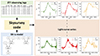 |
Fig. 1. Schematic representation of our simulation pipeline. Left: Model light curves are generated and combined with the true ZTF observing conditions to produce the simulated light curves. Right: comparison between our predicted dataset and the ZTF SN Ia DR2. |
This new framework was used to study the DR2 selection and its potential biases. To this end, skysurvey can be used to simulate the typical SNe Ia sample observed by the ZTF during its first phase by using its observed log file, that is, between March 2018 and December 2020, in the g, r, and i bands.
3.1. SN Ia model
To simulate an individual object, we first drew a redshift and sky position. To do this, we randomly selected a redshift from a non-evolving volumetric rate in the range 0 < z < 0.2, based on the Planck 2018 (Planck Collaboration VI 2020) fiducial cosmology (flat ΛCDM with H0 = 67.66 km s−1 Mpc−1 and Ωm = 0.30966) and a sky position (RA, Dec) within the ZTF footprint (Dekany et al. 2020). Skysurvey can be run in two ways: (i) By using a defined rate (by the default, the SN Ia rate is 2.35 × 10⁻⁴ Gpc−3 yr−1; Perley et al. 2020), or (ii) by specifying how many SNe Ia are to be simulated.
To generate a SN Ia light curve, we used the SALT2 time-dependent spectral energy distribution model (Guy et al. 2007, 2010). This template parametrises SNe Ia light curves by three parameters: t0, the epoch of maximum brightness in the B band, x1, the light-curve width, and c, the rest-frame colour. For our work described in Sect. 4, we used the observed properties of the SNe Ia gathered from the DR2 sample. To ensure that our light curves were representative of the overall SNe Ia population, we drew x1 in Sect. 5 from the distribution defined in Nicolas et al. (2021) using the parameters determined in Ginolin et al. (2024), and c from the parameter of Ginolin et al. (2025) for each event. t0 was drawn randomly within the ZTF-1 observing time range. For the light curves simulated in Sects. 4 and 5, we set the apparent peak luminosity in the B band, mB, by generating a peak absolute magnitude of −19.3, which was scattered using a colour-independent intrinsic dispersion of σint = 0.1–mag. We also corrected for the luminosity-decline rate and for the luminosity-colour relations with the nuisance parameters α = 0.14 and β = 3.15 from Betoule et al. (2014) via a Tripp relation (Tripp 1998). For each simulated event, we used the sncosmo framework (Barbary et al. 2016) to generate observer-frame light curves given the above information, and we included the effect of the Milky Way (MW) dust by using the extinction maps from Schlegel et al. (1998).
3.2. Observing logs
To match our generated model with the ZTF-1 survey, we compiled the observing conditions for every ZTF observation by querying the IPAC database. In particular, for every observation, we retrieved4
-
the date: mjdobs,
-
the sky location (observed field within the ZTF grid): fieldid,
-
the ZTF filter, CCD, and readout channel: fid, ccdid, and qid,
-
the processing status: infobits,
-
the zero-point magnitude of the observation: magzp,
-
the 5σ limiting magnitudes of the science image: scimaglim, and
-
the readout channel gain: gain.
We converted the measured limiting magnitude into an effective sky brightness (hereafter referred to as sky noise) using
 (1)
(1)
Our logs covered all observations from March 2018 to December 2020. A total of 431 000 exposures were retrieved, 37.1%, 55.5%, and 7.4 are in the g, r, and i bands, respectively.
3.3. Signal-to-noise ratio
The flux uncertainties for each simulated event have three contributions:
 (2)
(2)
where sb is the sky brightness (defined in Eq. (1)), f is the simulated flux, gain ≈ 6.2 is the CCD gain, and σcalib is the precision of the photometric calibration (Masci et al. 2019).
Before this framework was applied to free simulation, it was first tested on the DR2 targeted SNe Ia to confirm that the measured light curves can be reproduced with it. In order to estimate the accuracy of the simulations, we compared the simulated quantities of the DR2 light curves to the measured ones. The key quantity we used for this purpose is the signal-to-noise ratio (S/N), which is defined as
 (3)
(3)
where f and σf are the fluxes and their associated uncertainties, respectively, from Eq. (2). We computed the S/N of every DR2 object at each epoch of its measured and simulated light curve for each band (g, r, and i).
4. Testing the simulation framework
We describe how we validated the accuracy of skysurvey in reproducing the DR2 light curves below. By taking the real-time observing conditions and cadence of the ZTF and the observed properties of the objects gathered from the data into account, we aimed to replicate individual objects from the DR2 sample and compared the simulated and measured light curves. In Section 4.1 we describe the method we followed, in Section 4.2 we compare a simulated and measured light curve for one object of the sample, and in Section 4.3 we compare the fluxes, their uncertainties, and their S/N for the whole sample.
4.1. Method
To simulate the DR2 sample, we used the observed properties of the sample, that is, the SALT2 (Guy et al. 2007, 2010) fitted parameters of the measured light curves, as skysurvey inputs. The SALT2 parameters of the sample were presented in Rigault et al. (2025b). We used t0, x1, c, and z of every individual object in skysurvey combined with the ZTF observing logs to simulate every SN Ia. In order to evaluate the accuracy of our simulations, we compared the fluxes, flux uncertainties, and S/N of the simulated and measured light curves at all epochs for all DR2 objects. Furthermore, to avoid statistical fluctuations, each SN Ia was simulated ten times, that is, we generated about 30 000 SNe Ia for the whole DR2 sample.
4.2. One example
As an example, Fig. 2 shows the measured and simulated light curve of ZTF19abgppki in the g (left), r (middle), and i band (right). The top part of each plot shows the good agreement of the simulated and measured fluxes in all three bands at all epochs. We computed the S/N values of the simulated and measured light curves and their ratios. The bottom part of each plot in Fig. 2 shows the evolution of the S/N (S/Nsim/S/Ndata) as a function of time (in mjd) for the three bands. The crosses represent the median S/N values per observation. The S/N stand above one, especially for low fluxes at the starting point and in the tail of the light curves. This indicates that the simulated light curves have a higher S/N than the DR2 light curves. Because the fluxes seem to match in the upper part of the plots of Fig. 2, the simulated uncertainties do not reproduce the measured uncertainties. For a quantitative idea of the discrepancy and for the correction that needs to be applied to our simulations, a statistical analysis of all DR2 objects is necessary.
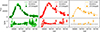 |
Fig. 2. An example of a simulated light-curve. Top: Simulated (ten times) and measured light curves (ZTF19abgppki, z = 0.06096) in the g (left), r (middle), and i (right) bands. Bottom: Evolution of the S/N of the simulated light curves with respect to the measured data points as a function of time (in mjd). The crosses show the median of the ten simulations for the S/N for each observation date. |
4.3. Statistical test of skysurvey
We applied the following set of basic cuts on the DR2 light-curve properties from Rigault et al. (2025a) to the 3628 SNe Ia of the entire DR2 sample
-
|x1|< 3,
-
c ∈ [ − 0.2, 0.8],
-
δt0 ≤ 1,
-
δx1 ≤ 1,
-
δc ≤ 0.1.
-
probfit > 10−7, and
-
we required data points with a phase (Φ) ∈[−10, 40].
We applied additional cuts of good sampling (they can be found in Rigault et al. 2025a). The phase cut was dictated by the study of DR2 light-curve residuals by Rigault et al. (2025b). The final sample consisted of 2662 SNe Ia. For the purpose of our study, we used this sample as our baseline. We simulated 2662 SNe Ia ten times with their SALT2 parameters and their redshift as inputs to skysurvey.
4.3.1. Comparison of the light curves
To ensure an accurate comparison of the measured and simulated quantities, we matched the measured and simulated light curve of each SN Ia and the associated observing logs.
The DR2 fluxes and associated uncertainties were extracted from the difference images, which are based on reference images, as discussed in the companion paper of Smith et al. (2025). We computed the flux uncertainties following Eq. (2) using sky noise derived from the difference-image limiting magnitudes or from the science-image limiting magnitudes. The ratio of the simulated uncertainties and the DR2 associated uncertainties (σsim/σdata) are shown in Fig. 3 for the three bands.
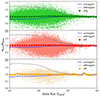 |
Fig. 3. Ratio of the simulated and DR2 flux uncertainties (σsim/σdata) as a function of data flux in the g (top), r (middle), and i (bottom) bands. The small points show the comparison between every simulated and observed object at every phase, and the larger points show the associated median binned values, both after correction for sky noise (see text for details). The blue curves (scimaglim) show the binned values obtained from the science image, and the grey curves (diffmaglim) show the binned values obtained from the difference-image limiting magnitudes, both without correction for sky noise. |
At low flux (typically f < 104), where the sky noise contribution (Eq. (2)) is dominant, the ratios of the simulated uncertainties that were computed with sky noise from the difference-image limiting magnitude are systematically above one, and the ratios of the uncertainties computed from the science limiting magnitude are systematically below one. Furthermore, the departure from one is more pronounced with the difference-image limiting magnitude, indicating that the associated sky noise is incorrectly estimated. When the sky noise was estimated using the science-image limiting magnitude, the simulated flux uncertainties are underestimated compared to the measured uncertainties, which is expected because the difference-image processing added some background noise, but the resulting values are more similar. This is a clear indication that a new estimated sky noise is required in the simulations to replicate the DR2 light curves accurately. To estimate the new sky noise, we used data points at low flux (f < 5000). We computed the median of the measured and simulated flux uncertainties for each flux range. By computing the median of the binned measured and simulated uncertainties, we obtained the corrective factor for the sky noise. A corrective factor of 1.23 for the g band, of 1.17 for the r band, and of 1.20 for the i band were required to solve the discrepancy between the simulated and measured uncertainties. This means that we needed to increase the sky-noise level associated with the science image to account for the forced photometry output that was applied to the difference images. To obtain the values of the new sky noise, we multiplied the sky noise obtained from the science limiting magnitude by the corrective factors we estimated for each of the three bands.
In addition, an error-floor uncertainty of 2.5%, 3.5%, and 6% of the flux level in the g, r, and i bands, respectively, was added to the DR2 flux uncertainties (Rigault et al. 2025b). In order to accurately compare the DR2 flux uncertainties to the simulated uncertaintiess, we needed to account for this error floor in the simulation framework.
We simulated our sample again with the correct prescription for the sky noise and the error floor. The ratio of the newly simulated uncertainties and the measured uncertainties for the sample are shown in the same figure (Fig. 3). We computed the median values for the ratios per flux range. They are represented in the same figure by the larger points. The data points are scattered around one, with larger scatter at low flux because sky noise dominates the flux uncertainties. The binned data points also lie between the ratio of the uncertainties computed with the science- and difference-image limiting magnitudes. The binned points are compatible with one along with their evolution with the flux, indicating that the newly simulated and the measured flux uncertainties agree well.
As discussed in Rigault et al. (2025b), an error floor is necessary to account for the Gaussian distribution of the light-curve data points with respect to the SALT2 model in the full fitted phase range [−10, 40]. The simulated fluxes were compared to the measured fluxes by computing the pull (fsim − fdata)/σdata for every point of the ten simulated light curves of the full DR2. Figure 4 shows the pull distribution for the three bands. The full histograms correspond to the pull computed by adding the error floor, and the open dashed histograms show the pull computed without the error floor. As the light-curve data points are distributed following a 1σ Gaussian centred on zero with respect to their SALT2 fitted model (see Fig. 1 of Rigault et al. 2025b, where σdata − pull = 1), and as the simulated light curves were generated following a random Gaussian distribution with respect to the SALT2 model (i.e. σsim − pull = 1), we expect a Gaussian distribution centred on zero for the pull of Fig. 4, with a σ equal to  . This prediction is represented in Fig. 4. The comparison of the expected and the computed pull agrees well when the error floor is taken into account (full histograms), but the computed pull distributions are wider when the error floor is omitted. This result shows that a level of the error floor of 2.5%, 3.5%, and 6% in the g, r, and i bands is necessary for a good match of the simulations and DR2 data.
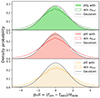 |
Fig. 4. Light-curve pulls (fluxsim–fluxdata)/σdata for the g (top), r (middle), and i (bottom) bands. The full (open dashed) histograms show the pulls with (without) error floor, and the grey curves correspond to a Gaussian centred on zero and with a σ equal to |

4.3.2. Comparison of the S/N
We used the newly simulated light curves with the prescriptions from Section 4.3.1 to compute the sky noise from the science limiting magnitudes with the correcting factors and the error floor needed in the flux uncertainties. We computed the S/N of the simulated and observed data points at all epochs, following Eq. (3). We represent the ratio of the S/N from the simulation and the DR2 as a function of the DR2 S/N in Fig. 5 for the g (top), r (middle), and i (bottom) bands. As shown in the figure, we computed the median of the S/N per S/N data range. The data points display a wider scatter especially at low S/N due to the sky noise fluctuations, which are dominant in the flux uncertainties budget at these S/N values. The scatter is reduced at higher S/N. The binned S/N are consistent with one in the three bands for S/N > 5. For the low S/N (< 5), the data points are below the detection limit and the S/N is affected by negative fluxes, so that the S/N (sim/data) = 1 is no longer valid. This shows that the simulation framework replicates the fluxes and associated uncertainties of the measured DR2 light curves at all epochs in the ZTF redshift range.
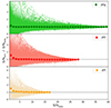 |
Fig. 5. S/N of simulated and DR2 as a function of DR2 S/N in the g (top), r (middle), and i (bottom) bands. The small points show the comparison between all simulated and observed objects at every phase, and the larger points show the associated median binned values. |
4.4. Summary
We simulated the most realistic DR2 SN Ia sample with all our knowledge of ZTF observations and SN Ia modeling. We used the ZTF true observing strategy and the most advanced SN Ia models in skysurvey to replicate the whole DR2 sample. We simulated 2662 SNe Ia that passed the good sampling and basic cuts, and we tested multiple configurations of the simulation framework. We replicated the DR2 fluxes, associated uncertainties, and S/N by using the sky noise computed from the science limiting magnitudes with a correction factor of 1.23 for the g band, 1.17 for the r band, and 1.20 for the i band. In addition, we accounted for an error floor of 2.5%, 3.5%, and 6% of the flux level in the g, r, and i band, respectively. With these prescriptions, we were able to simulate the ZTF DR2 SNIa light curves at all epochs accurately for every band (g, r, and i) up to the redshift limit of the survey of z ≈ 0.15.
5. Simulating the ZTF SN Ia DR2 sample
Simulations are crucial for correcting biases in the analysis of SNe Ia to infer cosmological quantities. In this section, we present our work on the DR2 selection sample with simulations.
5.1. ZTF SN Ia DR2 simulation
To study the selection effects on the DR2 sample, we carried out a high-statistics simulation. To avoid a limited sample at very low redshift, this simulation was partitioned into redshift bins with a width of 0.005 starting from 0 to 0.15, that is, we generated 25 000 SNe Ia in 30 redshift bins. In each bin, the SNe Ia were generated using the volumetric rate following the ΛCDM fiducial cosmology to compute the redshift dependence of the probed volume. To retrieve the realistic redshift dependence of the number of SNe Ia in the full redshift range (0 < z < 0.15), we applied a weight to each SN Ia depending on the initial redshift bin to reproduce the fiducial cosmological volumetric rate as a function of the redshift. This procedure is equivalent to simulating 400 million SNe Ia over the full redshift range (0 < z < 0.15). As mentioned in Sect. 3.1, we used the SALT2 to generate the light curves.
All selection cuts applied to the DR2 sample were reproduced for the simulated light curves. First, the selection function described in the ZTF SN Ia DR2 overview paper (Rigault et al. 2025a, Sect. 4.6) was applied to the generated light curves. This selection function was modeled by a survival sigmoid 1 − S(m; m0, s) = 1 − (1 + es(m − m0))−1 with a threshold m0 = 18.8 and a slope s = 4.5 that were applied to the peak magnitude of the light curve. Second, the basic DR2 cuts (see Table 1 of Rigault et al. 2025a) were applied to the fitted light curves. The next section describes the validation of the simulation framework.
5.2. Validating the simulation
Together, the selections cuts allowed us to reproduce the DR2 redshift distributions, as shown in Fig. 6. The natural redshift power law clearly decreased as a result of all selection cuts, so that we were able to reproduce the DR2 redshift distribution. The match is not perfect, but agrees very well. The two distributions are qualitatively the same. The high-redshift part (z > 0.07) indeed reproduces the drastic reduction mainly due to the selection function of up to a factor 100 at z = 0.15. Some structures appear in the DR2 data distribution, but not in the smooth evolution of the simulated distribution after the selection, especially in the redshift range 0.03 < z < 0.04. We did not identify the origin of this bump, but it might arise from the local large-scale structure of the Universe within the ZTF footprint or from an unmodeled population of underluminous SNeIa. A full analysis of the ZTF SNe Ia and the local large-scale structure must be carried out before we can draw any conclusion.
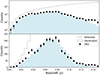 |
Fig. 6. Comparison of the DR2 redshift distribution (black points) with the skysurvey simulation in log scale (upper plot) and in linear scale (lower plot) from the generated SNe Ia distribution (dotted black line) to the selected distribution (blue full histograms). All simulated distributions (before and after the selection cuts) were normalised to the data sample. |
The simulated light-curve fit was conducted in the same way as for real data using the SALT2 model. A comparison of the main outputs from the SALT2 parameters is shown in Fig. 7 without a redshift cut (grey data points and light blue histogram for the simulation) and for z ≤ 0.06 (smaller black data points and blue histogram for the simulation). The three SALT2 output parameters are at first order well reproduced by the simulation, especially for the low-redshift selection z ≤ 0.06. We clearly observe the Malmquist bias for faint SNe Ia in the mb = −2.5log10(x0)+10.635 distribution (Fig. 7, upper plot). Compared to the low-redshift sample (z ≤ 0.06), the full sample shows a steeper distribution at high mb, which illustrates the selection effect for higher redshift. On the other hand, the shape of the stretch (x1; Fig. 7, middle plot) and the colour (c; Fig. 7, lower plot) distributions appear to be the same (at first order) for the full sample and for the low-redshift selection. A deeper analysis of the redshift dependence of these distributions is discussed in the next section.
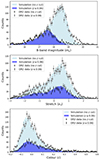 |
Fig. 7. Comparison of DR2 SALT2 parameters (points with error bars), mb (upper plot), x1 (middle plot), and c (lower plot), with the skysurvey SNe Ia simulation after the light-curve fit (histograms) without a redshift cut (grey points and light blue histogram) and for z ≤ 0.06 (smaller black points and blue histogram). |
To quantify the ability of the simulation to reproduce DR2 distributions, we computed a pseudo-χ2 per degree of freedom, defined as
 (4)
(4)
where Nbin is the number of bins in the compared histograms, which plays the role of the degree of freedom. In this definition, we assumed a Gaussian uncertainty for the data counting per bin ( ), and we neglected the statistical fluctuation of the simulation (the number of simulated SNe Ia that pass all selection cuts is 47 times that of the DR2 dataset). The limits of the histograms were defined by cutting 0.5% of the left and right tails of DR2 using the quantile method, that is, we kept 99% of the bulk of the distributions. For the robustness of the analysis, we varied Nbin from 80 to 100 in steps of one bin (i.e. 20 χ/ndf2 calculations for each distribution comparison), and then we computed the mean χ/ndf2 and evaluated the uncertainty on the mean value.
The results are presented in Table 1 for the three SALT2 parameters mb, x1, and c for the full DR2 sample (no z cut) and the lower-redshifts part (z ≤ 0.06). For the full data sample, the pseudo-χ2 per degree of freedom (χ/ndf2) is between 1.3 and 1.7, depending on the SALT2 parameter, which means that the simulations do not reproduce the full data set perfectly. The worst agreement is observed for the B-band magnitude (mB) parameter. The simulation misses the faintest objects. This is likely due to an underestimation of the selection, which was extrapolated beyond a peak magnitude of 19. When we compare DR2 and the simulated distributions for the lower-redshift part (z ≤ 0.06, which corresponds to what we call the volume-limited sample; see Sect. 5.3), we observe a small improvement for the mB distribution (even though the faintest objects are still missed). No improvement is seen for the stretch (x1) distributions, but a much better match is observed for the colour (c) distribution. This quantitative comparison shows that the simulation is close to reproducing the main properties of our SN Ia data sample for the volume-limited sample (z ≤ 0.06), which is described in more detail in the next section.
χ/ndf2 (with an estimate of its uncertainty) between DR2 and simulation distributions of SALT2 parameters mb, x1, and c for the full sample (no z cut) and for the volume-limited sample (z ≤ 0.06).
5.3. Volume-limited sample
An analysis of SALT2 parameters as a function of the redshift is necessary to estimate the limited redshift in which SNe Ia are not biased. Figure 8 shows a comparison of the input stretch (left plot) and colour (right plot) distributions before (filled grey histograms) and after selection cuts (open histograms). These plots show that the input distributions are well reproduced at very low redshift and start to be distorted when the redshift increased, typically beyond 0.06.
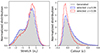 |
Fig. 8. Comparison of the stretch (left plot) and colour (right plot) input distributions before (filled grey histograms) and after all selection cuts (open histogram) for lower (z ≤ 0.06, open blue histogram) and higher redshifts (z > 0.06, open red histogram). |
A volume-limited sample can be defined as a data sample for which the input SALT2 distributions are not significantly distorted, meaning that there is no bias in the selected SNe Ia. To quantify the redshift limit of the volume-limited sample, we performed a Kolmogorov-Smirnov (KS) test between the input distributions used for the generation and the distributions retrieved after all selection cuts were applied to the simulated sample, as for real data, and as a function of redshift limit (z < zlim). The result of the KS test of the stretch (orange curves) and colour (red curves) parameters is shown in Fig. 9 and is compared to the probability limits at 1, 2, and 3σ. It shows that the colour distribution (red) is affected at a lower redshift limit than the stretch distribution (orange). The KS-test departure from 1σ corresponds to a redshift limit of about 0.08 for the stretch distribution, and it never reaches the 2σ level. For the colour distribution, the KS-test reaches 1, 2, and 3σ for the redshift limits of 0.05, 0.055, and 0.065, respectively (see also Table 2). We recall that the input colour distribution is a Gaussian shape (mean cint and sigma σc) convoluted with a decreasing exponential to describe the positive colour tail with the parameter τ. The colour distribution deduced from the volume-limited sample of the DR2 data was described in Ginolin et al. (2025) with the following parameters: cint = −0.085, σc = 0.03, and τ = 0.155. A study of the generated colour distribution after the selection cuts showed that the τ parameter is first affected by the redshift evolution described in Table 2. The 1, 2 and 3σ in the τ parameter follows (but does not correspond exactly to) the 1, 2, and 3σ limits in the KS test.
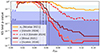 |
Fig. 9. KS-test p value for stretch (orange) and different colour distributions (red for Ginolin et al. 2025, dark red for Brout & Scolnic 2021, and salmon for Scolnic & Kessler 2016) as a function of the redshift limit (z < zlim). In each case, the KS-test is computed by comparing the generated distributions after and before the selection cuts. The dashed red line shows the result for Ginolin et al. (2025), but for c < 0.3. |
Evolution of the τ parameter of the colour distribution of selected SNe Ia as a function of the redshift limit. The τ value is compared to the input value τin = 0.155, and the uncertainty στ = 0.007 obtained in Ginolin et al. (2025) is taken into account.
The KS-test shows that the colour distribution is more sensitive to the selection cuts than the stretch distribution. To consolidate this analysis, we therefore ran two independent high-statistics simulations by using alternative colour distributions: (i) with the same analytical function as in Brout & Scolnic (2021), but with different parameters cint = −0.084, σc = 0.042, and τ = 0.10 (called Brout 2021 in the text below), and (ii) with the asymmetrical Gaussian shape from Scolnic & Kessler (2016) with  , σ− = 0.03, and σ+ = 0.1 (called Scolnic 2016 in the text below). These two alternative colour distributions are compared to our baseline distribution (Ginolin et al. 2025) in Fig. 10.
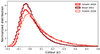 |
Fig. 10. Comparison of the colour distributions from Ginolin et al. (2025) (red) with those from Brout & Scolnic (2021) (dark red, with parametrisation (i), see text) and Scolnic & Kessler (2016) (salmon, with parametrisation (ii), see text). |
The KS-test result for these two distributions is presented in Fig. 9 (dark red for Brout 2021 and salmon for Scolnic 2016) and is then compared to our baseline (Ginolin et al. 2025) result (red, called Ginolin 2024 in the text). The KS-test result with the Brout 2021 parametrisation is smoother at a higher redshift limit than the KS-test performed with our baseline. This is expected because the high-colour tail decreases more quickly with the Brout 2021 parametrisation. When compared to the Scolnic 2016 distribution, which uses a different analytical form, the KS-test results are more similar because the behaviour of the high-colour tail is similar to our baseline distribution. This means, as discussed previously with the correlation to the τ parameter of the Ginolin 2024 distribution, that the bulk of the colour distribution, typically |c|< 0.2, does not drive the redshift limit that is used to define the volume-limited sample. The redshift limits of the KS-test values at 2σ are 0.055, 0.062, and 0.06 for the Ginolin 2024, Brout 2021, and Scolnic 2016 distributions, respectively. The Ginolin 2024 colour distribution therefore appears to be the most conservative at 2σ, and the redshift limit zlim = 0.06 corresponds to a 2.2σ effect for the Ginolin 2024 and Scolnic 2016 colour distributions.
Furthermore, as cosmological analysis are usually performed with SNe Ia light curves that are selected with a colour parameter |c|< 0.3 (Scolnic et al. 2018), the impact of the tail is weaker. We therefore performed the KS-test with our baseline colour distribution, but we compared the selected SNe Ia with c < 0.3 to the generated SNe Ia with c < 0.3. The result is shown with the dashed red line in Fig. 9. In this case, the redshift limit at 1σ and 2σ in the KS-test reaches a typical value of 0.07 and 0.85, respectively. This shows that the end part of the tail of the colour distribution drives the KS-test result. Because the fraction of SNe Ia in the last part of the tail (c > 0.3) is relatively small (8% with our baseline distribution), the redshift limit zlim = 0.06 seems to be a good choice to define the volume-limited sample for astrophysical studies.
We therefore conclude from this analysis that a very robust redshift limit of the volume-limited sample within 1σ for the KS-test (i.e. due to statistical fluctuations) is zlim = 0.05 for all SALT2 parameter ranges (x1 and c). Nevertheless, an extension up to a redshift limit zlim = 0.06 appears to be relatively reliable, and this limit can be pushed to zlim = 0.08 for a cosmological analysis.
6. Toward a cosmological analysis
The simulation framework was tested up to the Hubble-Lemaître diagram. To this end, the distance modulus of the fitted SNe Ia of the high-statistic simulation was computed by assuming the fiducial input parameters for the standardisation: μi = mb, i − (Mb − α x1, i + β ci) for every (i) SN Ia with Mb = −19.3, α = 0.14, and β = 3.15. We then deduced the residuals to the fiducial input cosmology (Planck 2018; Planck Collaboration VI 2020), Δμi = μi − μ(zi), where μ(zi) is the theoretical result of the fiducial cosmology for every SN Ia redshift zi.
The residual distribution is presented in Fig. 11 with a comparison of the DR2 data (2624 SNeIa) and the simulation with the fitted and generated SALT2 parameters (full and open histograms). Firstly, the dispersion of the fitted residual distribution is similar to the generated distribution, which indicatees that the residual is mainly driven by intrinsic dispersion (σint). Secondly, the fitted simulation reproduces the distribution measured from the DR2 dataset overall (χ/ndf2 = 2.00), with small discrepancies that we will solve in the upcoming DR2.5 cosmological data release. The robust agreement of our simulated samples and the DR2 dataset for the volume-limited sample, with χ/ndf2 = 1.55, 1.30, 1.28, and 1.63 for the distribution of mB, x1, c, and Δμ, respectively, indicates that the underlying distribution of the parameters and the selection of events are well understood. This lays the foundations for a cosmological analysis.
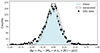 |
Fig. 11. Hubble-Lemaître diagram of the residual distribution, assuming no environmental steps, for the DR2 (black points), and for the simulation with the fitted and generated SALT2 parameters (full and open histograms). |
The DR2 dataset (and other literature samples) have observed significant correlations between the residual luminosity, the standardisation parameters, and the measures of the local environment (e.g. Ginolin et al. 2024, 2025). To ensure that our estimates of the cosmological parameters are unbiased, these must be included in our simulation framework, which must also be updated to match the reprocessed scene-model photometry (SMP) (Lacroix et al., in prep.), and it must be benchmarked against widely used software, for example SNANA. This work will be released as part of the DR2.5 cosmological analysis, which is due for release in late 2025.
7. Conclusion
We presented the performance of the simulation framework, skysurvey and its advanced version skysurvey, that was developed for the ZTF survey. The targeted simulation of the first phase of the ZTF, from March 2018 to December 2020, was used to validate the full pipeline. The comparison to the ZTF SN Ia DR2 sample showed that neither the science- nor the difference-image magnitude limit are able to reproduce the measured flux uncertainties. A tuning of the sky noise with an increasing factor of 1.23, 1.17, and 1.20 for the g, r, and i bands, respectively, was derived to match the flux uncertainties for the science-image magnitude limit with an additional calibration error of 2.5%, 3.5%, and 6% for the g, r, and i bands. The simulation using the realistic SALT2 stretch and colour distribution showed the ability of the skysurvey package to reproduce the ZTF SN Ia DR2 sample. Finally, a redshift study of the SALT2 parameters allowed us to identify a volume-limited sample, z ≤ 0.06, that is, an unbiased sample of about 1000 SNe Ia. This volume-limited sample is unique, and new studies of SNe Ia can be based on this sample, especially an analysis to improve their standardisation procedure for future cosmological analyses. Moreover, this redshift limit can be pushed up to z ≤ 0.08 for a cosmological analysis when the reddes SNe Ia (c < 0.3) are removed, which increases the statistics to almost 1700 SNe Ia. This unbiased low-redshift SN Ia sample is invaluable for conducting new astrophysical and cosmological studies.
See https://sites.astro.caltech.edu/ztf/bts/explorer.php for the latest values.
See Masci et al. (2017) for a description of all available columns.
Acknowledgments
Based on observations obtained with the Samuel Oschin Telescope 48-inch and the 60-inch Telescope at the Palomar Observatory as part of the Zwicky Transient Facility project. ZTF is supported by the National Science Foundation under Grant No. AST-1440341 and a collaboration including Caltech, IPAC, the Weizmann Institute of Science, the Oskar Klein Center at Stockholm University, the University of Maryland, the University of Washington, Deutsches Elektronen-Synchrotron and Humboldt University, Los Alamos National Laboratories, the TANGO Consortium of Taiwan, the University of Wisconsin at Milwaukee, and Lawrence Berkeley National Laboratories. Operations are conducted by COO, IPAC, and UW. The ZTF forced-photometry service was funded under the Heising-Simons Foundation grant #12540303 (PI: Graham). SED Machine is based upon work supported by the National Science Foundation under Grant No. 1106171 This work was supported by the GROWTH project (Kasliwal et al. 2019) funded by the National Science Foundation under Grant No 1545949. This project has received funding from the European Research Council (ERC) under the European Union’s Horizon 2020 research and innovation programme (grant agreement n 759194 – USNAC). P.R. acknowledges the support received from the Agence Nationale de la Recherche of the French government through the program ANR-21-CE31-0016-03. UB is supported by the H2020 European Research Council grant no. 758638 GD is supported by the H2020 European Research Council grant no. 758638 L.G. acknowledges financial support from AGAUR, CSIC, MCIN and AEI 10.13039/501100011033 under projects PID2020-115253GA-I00, PIE 20215AT016, CEX2020-001058-M, and 2021-SGR-01270. This work has been supported by the research project grant “Understanding the Dynamic Universe” funded by the Knut and Alice Wallenberg Foundation under Dnr KAW 2018.0067 and the Vetenskapsrådet, the Swedish Research Council, project 2020-03444 LH is funded by the Irish Research Council under grant number GOIPG/2020/1387 Y.-L.K. has received funding from the Science and Technology Facilities Council [grant number ST/V000713/1] KM is supported by the H2020 European Research Council grant no. 758638. T.E.M.B. acknowledges financial support from the Spanish Ministerio de Ciencia e Innovación (MCIN) and the Agencia Estatal de Investigación (AEI) 10.13039/501100011033 under the PID2020-115253GA-I00 HOSTFLOWS project, and from Centro Superior de Investigaciones Científicas (CSIC) under the PIE project 20215AT016 and the program Unidad de Excelencia María de Maeztu CEX2020-001058-M. JHT is supported by the H2020 European Research Council grant no. 758638.
References
- Aubert, M., Rosnet, P., Popovic, B., et al. 2025, A&A, 694, A7 (ZTF DR2 SI) [NASA ADS] [CrossRef] [EDP Sciences] [Google Scholar]
- Barbary, K., Barclay, T., Biswas, R., et al. 2016, Astrophysics Source Code Library [record ascl:1611.017] [Google Scholar]
- Bellm, E. C., Kulkarni, S. R., Graham, M. J., et al. 2019, PASP, 131, 018002 [Google Scholar]
- Betoule, M., Kessler, R., Guy, J., et al. 2014, A&A, 568, A22 [NASA ADS] [CrossRef] [EDP Sciences] [Google Scholar]
- Blagorodnova, N., Neill, J. D., Walters, R., et al. 2018, PASP, 130, 035003 [Google Scholar]
- Brout, D., & Scolnic, D. 2021, ApJ, 909, 26 [NASA ADS] [CrossRef] [Google Scholar]
- Brout, D., Scolnic, D., Popovic, B., et al. 2022, ApJ, 938, 110 [NASA ADS] [CrossRef] [Google Scholar]
- Burgaz, U., Maguire, K., Dimitriadis, G., et al. 2025a, A&A, 694, A13 (ZTF DR2 SI) [NASA ADS] [CrossRef] [EDP Sciences] [Google Scholar]
- Burgaz, U., Maguire, K., Dimitriadis, G., et al. 2025b, A&A, 694, A9 (ZTF DR2 SI) [NASA ADS] [CrossRef] [EDP Sciences] [Google Scholar]
- Carreres, B., Bautista, J. E., Feinstein, F., et al. 2023, A&A, 674, A197 [NASA ADS] [CrossRef] [EDP Sciences] [Google Scholar]
- Carreres, B., Rosselli, D., Bautista, J. E., et al. 2025, A&A, 694, A8 (ZTF DR2 SI) [NASA ADS] [CrossRef] [EDP Sciences] [Google Scholar]
- De, K., Kasliwal, M. M., Tzanidakis, A., et al. 2020, ApJ, 905, 58 [NASA ADS] [CrossRef] [Google Scholar]
- Deckers, M., Maguire, K., Shingles, L., et al. 2025, A&A, 694, A12 (ZTF DR2 SI) [NASA ADS] [CrossRef] [EDP Sciences] [Google Scholar]
- Dekany, R., Smith, R. M., Riddle, R., et al. 2020, PASP, 132, 038001 [NASA ADS] [CrossRef] [Google Scholar]
- Dhawan, S., Goobar, A., Smith, M., et al. 2022, MNRAS, 510, 2228 [NASA ADS] [CrossRef] [Google Scholar]
- Dhawan, S., Mortsell, E., Johansson, J., et al. 2024, A&A, submitted [arXiv:2406.01434] (ZTF DR2 SI) [Google Scholar]
- Dimitriadis, G., Burgaz, U., Deckers, M., et al. 2025, A&A, 694, A10 (ZTF DR2 SI) [NASA ADS] [CrossRef] [EDP Sciences] [Google Scholar]
- Feindt, U., Nordin, J., Rigault, M., et al. 2019, JCAP, 2019, 005 [CrossRef] [Google Scholar]
- Fremling, C., Miller, A. A., Sharma, Y., et al. 2020, ApJ, 895, 32 [NASA ADS] [CrossRef] [Google Scholar]
- Ginolin, M., Rigault, M., Smith, M., et al. 2024, A&A, submitted [arXiv:2405.20965] (ZTF DR2 SI) [Google Scholar]
- Ginolin, M., Rigault, M., Copin, Y., et al. 2025, A&A, 694, A4 (ZTF DR2 SI) [NASA ADS] [CrossRef] [EDP Sciences] [Google Scholar]
- Graham, M. J., Kulkarni, S. R., Bellm, E. C., et al. 2019, PASP, 131, 078001 [Google Scholar]
- Gris, P., Regnault, N., Awan, H., et al. 2023, ApJS, 264, 22 [NASA ADS] [CrossRef] [Google Scholar]
- Guy, J., Astier, P., Baumont, S., et al. 2007, A&A, 466, 11 [NASA ADS] [CrossRef] [EDP Sciences] [Google Scholar]
- Guy, J., Sullivan, M., Conley, A., et al. 2010, A&A, 523, A7 [NASA ADS] [CrossRef] [EDP Sciences] [Google Scholar]
- Johansson, J., Smith, M., Rigault, M., et al. 2025, A&A in prep. (ZTF DR2 SI) [Google Scholar]
- Kasliwal, M. M., Cannella, C., Bagdasaryan, A., et al. 2019, PASP, 131, 038003 [NASA ADS] [CrossRef] [Google Scholar]
- Kessler, R., Bernstein, J. P., Cinabro, D., et al. 2009, PASP, 121, 1028 [Google Scholar]
- Kessler, R., Brout, D., D’Andrea, C. B., et al. 2019, MNRAS, 485, 1171 [NASA ADS] [CrossRef] [Google Scholar]
- Kim, Y. L., Rigault, M., Neill, J. D., et al. 2022, PASP, 134, 024505 [NASA ADS] [CrossRef] [Google Scholar]
- Magee, M. R., Cuddy, C., Maguire, K., et al. 2022, MNRAS, 513, 3035 [NASA ADS] [CrossRef] [Google Scholar]
- Masci, F. J., Laher, R. R., Rebbapragada, U. D., et al. 2017, PASP, 129, 014002 [NASA ADS] [CrossRef] [Google Scholar]
- Masci, F. J., Laher, R. R., Rusholme, B., et al. 2019, PASP, 131, 018003 [Google Scholar]
- Nicolas, N., Rigault, M., Copin, Y., et al. 2021, A&A, 649, A74 [NASA ADS] [CrossRef] [EDP Sciences] [Google Scholar]
- Patterson, M. T., Bellm, E. C., Rusholme, B., et al. 2019, PASP, 131, 018001 [Google Scholar]
- Perley, D. A., Fremling, C., Sollerman, J., et al. 2020, ApJ, 904, 35 [NASA ADS] [CrossRef] [Google Scholar]
- Planck Collaboration VI. 2020, A&A, 641, A6 [NASA ADS] [CrossRef] [EDP Sciences] [Google Scholar]
- Popovic, B., Rigault, M., Smith, M., et al. 2025, A&A, 694, A5 (ZTF DR2 SI) [NASA ADS] [CrossRef] [EDP Sciences] [Google Scholar]
- Rigault, M., Neill, J. D., Blagorodnova, N., et al. 2019, A&A, 627, A115 [NASA ADS] [CrossRef] [EDP Sciences] [Google Scholar]
- Rigault, M., Smith, M., Goobar, A., et al. 2025a, A&A, 694, A1 (ZTF DR2 SI) [NASA ADS] [CrossRef] [EDP Sciences] [Google Scholar]
- Rigault, M., Smith, M., Regnault, N., et al. 2025b, A&A, 694, A2 (ZTF DR2 SI) [NASA ADS] [CrossRef] [EDP Sciences] [Google Scholar]
- Ruppin, F., Rigault, M., Ginolin, M., et al. 2025, A&A, 694, A6 (ZTF DR2 SI) [NASA ADS] [CrossRef] [EDP Sciences] [Google Scholar]
- Sagués Carracedo, A., Bulla, M., Feindt, U., & Goobar, A. 2021, MNRAS, 504, 1294 [CrossRef] [Google Scholar]
- Schlegel, D. J., Finkbeiner, D. P., & Davis, M. 1998, ApJ, 500, 525 [Google Scholar]
- Scolnic, D., & Kessler, R. 2016, ApJ, 822, L35 [Google Scholar]
- Scolnic, D. M., Jones, D. O., Rest, A., et al. 2018, ApJ, 859, 101 [NASA ADS] [CrossRef] [Google Scholar]
- Smartt, S. J., Valenti, S., Fraser, M., et al. 2015, A&A, 579, A40 [NASA ADS] [CrossRef] [EDP Sciences] [Google Scholar]
- Smith, M., Rigault, M., et al. 2025, A&A in prep. (ZTF DR2 SI) [Google Scholar]
- Tripp, R. 1998, A&A, 331, 815 [NASA ADS] [Google Scholar]
- Vincenzi, M., Brout, D., Armstrong, P., et al. 2024, ArXiv e-prints [arXiv:2401.02945] [Google Scholar]
All Tables
χ/ndf2 (with an estimate of its uncertainty) between DR2 and simulation distributions of SALT2 parameters mb, x1, and c for the full sample (no z cut) and for the volume-limited sample (z ≤ 0.06).
Evolution of the τ parameter of the colour distribution of selected SNe Ia as a function of the redshift limit. The τ value is compared to the input value τin = 0.155, and the uncertainty στ = 0.007 obtained in Ginolin et al. (2025) is taken into account.
All Figures
|
Fig. 1. Schematic representation of our simulation pipeline. Left: Model light curves are generated and combined with the true ZTF observing conditions to produce the simulated light curves. Right: comparison between our predicted dataset and the ZTF SN Ia DR2. |
| In the text | |
|
Fig. 2. An example of a simulated light-curve. Top: Simulated (ten times) and measured light curves (ZTF19abgppki, z = 0.06096) in the g (left), r (middle), and i (right) bands. Bottom: Evolution of the S/N of the simulated light curves with respect to the measured data points as a function of time (in mjd). The crosses show the median of the ten simulations for the S/N for each observation date. |
| In the text | |
|
Fig. 3. Ratio of the simulated and DR2 flux uncertainties (σsim/σdata) as a function of data flux in the g (top), r (middle), and i (bottom) bands. The small points show the comparison between every simulated and observed object at every phase, and the larger points show the associated median binned values, both after correction for sky noise (see text for details). The blue curves (scimaglim) show the binned values obtained from the science image, and the grey curves (diffmaglim) show the binned values obtained from the difference-image limiting magnitudes, both without correction for sky noise. |
| In the text | |
|
Fig. 4. Light-curve pulls (fluxsim–fluxdata)/σdata for the g (top), r (middle), and i (bottom) bands. The full (open dashed) histograms show the pulls with (without) error floor, and the grey curves correspond to a Gaussian centred on zero and with a σ equal to |
| In the text | |
|
Fig. 5. S/N of simulated and DR2 as a function of DR2 S/N in the g (top), r (middle), and i (bottom) bands. The small points show the comparison between all simulated and observed objects at every phase, and the larger points show the associated median binned values. |
| In the text | |
|
Fig. 6. Comparison of the DR2 redshift distribution (black points) with the skysurvey simulation in log scale (upper plot) and in linear scale (lower plot) from the generated SNe Ia distribution (dotted black line) to the selected distribution (blue full histograms). All simulated distributions (before and after the selection cuts) were normalised to the data sample. |
| In the text | |
|
Fig. 7. Comparison of DR2 SALT2 parameters (points with error bars), mb (upper plot), x1 (middle plot), and c (lower plot), with the skysurvey SNe Ia simulation after the light-curve fit (histograms) without a redshift cut (grey points and light blue histogram) and for z ≤ 0.06 (smaller black points and blue histogram). |
| In the text | |
|
Fig. 8. Comparison of the stretch (left plot) and colour (right plot) input distributions before (filled grey histograms) and after all selection cuts (open histogram) for lower (z ≤ 0.06, open blue histogram) and higher redshifts (z > 0.06, open red histogram). |
| In the text | |
|
Fig. 9. KS-test p value for stretch (orange) and different colour distributions (red for Ginolin et al. 2025, dark red for Brout & Scolnic 2021, and salmon for Scolnic & Kessler 2016) as a function of the redshift limit (z < zlim). In each case, the KS-test is computed by comparing the generated distributions after and before the selection cuts. The dashed red line shows the result for Ginolin et al. (2025), but for c < 0.3. |
| In the text | |
|
Fig. 10. Comparison of the colour distributions from Ginolin et al. (2025) (red) with those from Brout & Scolnic (2021) (dark red, with parametrisation (i), see text) and Scolnic & Kessler (2016) (salmon, with parametrisation (ii), see text). |
| In the text | |
|
Fig. 11. Hubble-Lemaître diagram of the residual distribution, assuming no environmental steps, for the DR2 (black points), and for the simulation with the fitted and generated SALT2 parameters (full and open histograms). |
| In the text | |
Current usage metrics show cumulative count of Article Views (full-text article views including HTML views, PDF and ePub downloads, according to the available data) and Abstracts Views on Vision4Press platform.
Data correspond to usage on the plateform after 2015. The current usage metrics is available 48-96 hours after online publication and is updated daily on week days.
Initial download of the metrics may take a while.