| Issue |
A&A
Volume 695, March 2025
ZTF SN Ia DR2
|
|
|---|---|---|
| Article Number | A140 | |
| Number of page(s) | 16 | |
| Section | Cosmology (including clusters of galaxies) | |
| DOI | https://doi.org/10.1051/0004-6361/202450378 | |
| Published online | 14 March 2025 | |
ZTF SN Ia DR2: Environmental dependencies of stretch and luminosity for a volume-limited sample of 1000 type Ia supernovae
1
Univ Lyon, Univ Claude Bernard Lyon 1, CNRS, IP2I Lyon/IN2P3, UMR 5822, F-69622 Villeurbanne, France
2
Department of Physics, Lancaster University, Lancs LA1 4YB, UK
3
School of Physics, Trinity College Dublin, College Green, Dublin 2, Ireland
4
Oskar Klein Centre, Department of Physics, Stockholm University, SE-10691 Stockholm, Sweden
5
Institut für Physik, Humboldt Universität zu Berlin, Newtonstr 15, 12101 Berlin, Germany
6
National Research Council of Canada, Herzberg Astronomy & Astrophysics Research Centre, 5071 West Saanich Road, Victoria, BC V9E 2E7, Canada
7
Université Clermont Auvergne, CNRS/IN2P3, LPCA, F-63000 Clermont-Ferrand, France
8
Sorbonne Université, CNRS/IN2P3, LPNHE, F-75005 Paris, France
9
Aix Marseille Université, CNRS/IN2P3, CPPM, Marseille, France
10
Department of Physics, Duke University, Durham, NC 27708, USA
11
Institute of Astronomy and Kavli Institute for Cosmology, University of Cambridge, Madingley Road, Cambridge CB3 0HA, UK
12
Institute of Space Sciences (ICE, CSIC), Campus UAB, Carrer de Can Magrans, s/n, E-08193 Barcelona, Spain
13
Institut d’Estudis Espacials de Catalunya (IEEC), E-08034 Barcelona, Spain
14
Deutsches Elektronen Synchrotron DESY, Platanenallee 6, 15738 Zeuthen, Germany
15
Lawrence Berkeley National Laboratory, 1 Cyclotron Road, MS, 50B-4206 Berkeley, CA 94720, USA
16
Department of Astronomy, University of California, Berkeley, 501 Campbell Hall, Berkeley, CA 94720, USA
17
Oskar Klein Centre, Department of Astronomy, Stockholm University, SE-10691 Stockholm, Sweden
18
Nordic Optical Telescope, Rambla José Ana Fernández Pérez 7, ES-38711 Breña Baja, Spain
19
Caltech Optical Observatories, California Institute of Technology, Pasadena, CA 91125, USA
20
DIRAC Institute, Department of Astronomy, University of Washington, 3910 15th Avenue NE, Seattle, WA 98195, USA
21
Division of Physics, Mathematics, and Astronomy, California Institute of Technology, Pasadena, CA 91125, USA
22
IPAC, California Institute of Technology, 1200 E. California Blvd, Pasadena, CA 91125, USA
⋆ Corresponding author; This email address is being protected from spambots. You need JavaScript enabled to view it.
Received:
15
April
2024
Accepted:
31
January
2025
Abstract
Context. Type Ia supernova (SN Ia) cosmology studies will soon be dominated by systematic, uncertainties, rather than statistical ones. Thus, it is crucial to understand the unknown phenomena potentially affecting their luminosity that may remain, such as astrophysical biases. For their accurate application in such studies, SN Ia magnitudes need to be standardised; namely, they must be corrected for their correlation with the light-curve width and colour.
Aims. Here, we investigate how the standardisation procedure used to reduce the scatter of SN Ia luminosities is affected by their environment. Our aim is to reduce scatter and improve the standardisation process.
Methods. We first studied the SN Ia stretch distribution, as well as its dependence on environment, as characterised by local and global (g − z) colour and stellar mass. We then looked at the standardisation parameter, α, which accounts for the correlation between residuals and stretch, along with its environment dependency and linearity. Finally, we computed the magnitude offsets between SNe in different astrophysical environments after the colour and stretch standardisations (i.e. steps). This analysis has been made possible thanks to the unprecedented statistics of the volume-limited Zwicky Transient Facility (ZTF) SN Ia DR2 sample.
Results. The stretch distribution exhibits a bimodal behaviour, as previously found in the literature. However, we find the distribution to be dependent on environment. Specifically, the mean stretch modes decrease with host stellar mass, at a 9.2σ significance. We demonstrate, at the 13.4σ level, that the stretch-magnitude relation is non-linear, challenging the usual linear stretch-residuals relation currently used in cosmological analyses. In fitting for a broken-α model, we did indeed find two different slopes between stretch regimes (x1 ≶ x10 with x10 = −0.48 ± 0.08): αlow = 0.271 ± 0.011 and αhigh = 0.083 ± 0.009, comprising a difference of Δα = −0.188 ± 0.014. As the relative proportion of SNe Ia in the high-stretch and low-stretch modes evolves with redshift and environment, this implies that a single-fitted α also evolves with the redshift and environment. Concerning the environmental magnitude offset γ, we find it to be greater than 0.12 mag, regardless of the considered environmental tracer used (local or global colour and stellar mass), all measured at the ≥5σ level. When accounting for the non-linearity of the stretch, these steps increase to ∼0.17 mag, measured with a precision of 0.01 mag. Such strong results highlight the importance of using a large volume-limited dataset to probe the underlying SN Ia-host correlations.
Key words: supernovae: general / dark energy
© The Authors 2025
 Open Access article, published by EDP Sciences, under the terms of the Creative Commons Attribution License (https://creativecommons.org/licenses/by/4.0), which permits unrestricted use, distribution, and reproduction in any medium, provided the original work is properly cited.
This article is published in open access under the Subscribe to Open model. This email address is being protected from spambots. You need JavaScript enabled to view it. to support open access publication.
1. Introduction
Type Ia supernovae (SNe Ia) are standardisable candles that have enabled the discovery of the acceleration of the Universe’s expansion in the late 1990s (Riess et al. 1998; Perlmutter et al. 1999). Today, they remain a key cosmological probe, as they are uniquely able to measure the recent (z < 0.5) expansion rate of the Universe and, as such, they are key to deriving the dark energy equation of state parameter, w (Planck Collaboration VI 2020; Brout et al. 2022), along with its potential evolution with redshift and the direct measurement of the Hubble-Lemaétre constant, H0 (Freedman 2021; Riess et al. 2022).
The state-of-the-art measurements of cosmological parameters show that a cosmological constant Λ explains the observed properties of dark energy with w compatible with −1 at the 3% precision level (Betoule et al. 2014; Scolnic et al. 2018; Brout et al. 2022). However, the direct measurement of H0 is incompatible at the 5σ level with the standard model, Λ cold dark matter (ΛCDM) when the parameters are anchored by early Universe physics (Macaulay et al. 2019; Feeney et al. 2019; Riess et al. 2022). If the latter is not caused by (necessarily multiple, see Riess et al. 2022) sources of systematic uncertainties, this tension would be a sign of new fundamental physics. Yet, no simple theoretical deviation to the fiducial model is able to explain this tension without creating other issues (see Schöneberg et al. 2022, for a recent review). In that context, it is necessary to further investigate the existence of systematic biases that may affect distances derived from SN Ia data.
SNe Ia, as ‘standardisable’ candles, have a natural scatter of ∼0.40 mag. However, two empirical relations, namely, the so-called slower-brighter and bluer-brighter relations (Phillips 1993; Tripp 1998) make use of SN Ia light-curve properties to reduce that scatter down to ∼0.15 mag. The SALT (Guy et al. 2007, 2010; Betoule et al. 2014) light-curve fitter is the usual algorithm used to estimate SN Ia light-curve stretch, x1, and colour parameter, c (see Kenworthy et al. (2021) and Augarde et al. (in prep.) for a recent re-coding).
The significantly reduced scatter provided by these two linear relations makes SNe Ia the best cosmological distance indicator. Yet, only half of this remaining scatter can be explained by known measurement errors or modelling uncertainties. The rest, dubbed intrinsic scatter, may be due to unknown systematic uncertainties that could bias distances and, as a result, the measurement of cosmological parameters.
It has been demonstrated that SN Ia properties do vary as a function of their environment. The light-curve stretch, a purely intrinsic property, has been shown to depend on the host environment, such that older and redder environments host (on average) faster evolving SNe Ia (e.g. Filippenko 1989; Hamuy et al. 1996; Sullivan et al. 2010; Rigault et al. 2020). Since the galactic star formation quickly evolves with redshift (Madau & Dickinson 2014), it has been suggested that SN Ia intrinsic properties evolve with redshift (Howell et al. 2007), as recently demonstrated at the 5σ level by Nicolas et al. (2021). Yet, as long as the stretch brightness dependency is fully captured by the standardisation procedure, such an intrinsic redshift evolution of SN Ia properties should not affect SN Ia cosmology, apart for when the actual stretch distribution is needed; for instance, for selection effect bias corrections (Scolnic & Kessler 2016).
However, it has been shown that SNe Ia from massive hosts are on average brighter after standardisation than these from low-mass hosts (Kelly et al. 2010; Sullivan et al. 2010; Lampeitl et al. 2010; Childress et al. 2013; Rigault et al. 2020). This so called ‘mass step’ is now accounted for in cosmological analyses (Betoule et al. 2014; Scolnic et al. 2018; Brout et al. 2022; Popovic et al. 2024), but its origin is highly debated. Research suggests that it could be due to progenitor age (e.g. Rigault et al. 2020; Briday et al. 2021; Kim et al. 2018) or dust property variations (e.g. Brout & Scolnic 2021; Popovic et al. 2021, 2023). Understanding the origin of such variations is required for accurate cosmology, since corrections for redshift evolution or sample selection functions may vary with environment.
In this analysis, we investigate the stretch standardisation procedure, its connection with the mass step, and the relation between SN stretch and progenitor age. In a companion paper (Ginolin et al. 2025), we focus on SN Ia colour, its potential connection with dust, and the accuracy of the colour standardisation. Both papers are based on the second data release of the Zwicky Transient Facility (ZTF; Bellm et al. 2019; Graham et al. 2019; Dekany et al. 2020; Masci et al. 2019) Cosmology Science Working Group (ZTF SN Ia DR2, Rigault et al. 2025a; Smith et al. 2025, following the DR1, Dhawan et al. 2022).
This paper starts in Sect. 2 with a summary of the ZTF SN Ia DR2 release, where we introduce the sample selection used to create a well controlled volume-limited dataset. In Sect. 3, we study the stretch distribution, where we present a more complex connection between SN stretch and SN environment than what has been previously reported. In Sect. 4, we investigate in detail the stretch-magnitude relation, which we find to be significantly non-linear. In Sect. 5 we then investigate magnitude offsets due to SN environment (i.e. steps), as well as their connection to the non-linearity of the stretch-residuals relation. We test the robustness of our results in Sect. 6.1, discuss our results in Sect. 6, and present our conclusions in Sect. 7. Unless otherwise mentioned, we used the recent recalibration of the SALT2.4 light-curve fitter (Guy et al. 2010; Betoule et al. 2014) from Taylor et al. (2021) as provided by the ZTF SN Ia DR2 release, following Rigault et al. (2025a); Smith et al. (2025).
2. Data
2.1. Zwicky Transient Facility Cosmology DR2
For this analysis, we used the volume-limited ZTF SN Ia DR2 sample presented in Rigault et al. (2025a); Smith et al. (2025). The initial DR2 sample contains 2663 spectroscopically confirmed SNe Ia passing basic quality cuts: (1) Good light-curve sampling, namely, at least seven 5σ flux detections within the −10 to +40 days rest-frame phase range, with at least two pre-max detections, at least two post-max detections, and at least one detection in two bands; (2) stretch x1 ∈ [3, 3] measured with a precision better than σx1 = 1; (3) colour c ∈ [ − 0.2, 0.8] measured with a precision better than σc = 0.1; (4) precision on the estimated peak-luminosity time better than σt0 = 1 day; and (5) SALT2 light-curve fit probability greater than 10−7. Finally, to obtain a volume-limited sample, we limited ourselves to SNe Ia with a redshift of z < 0.06, following the prescription from survey simulations (Amenouche et al. 2025), so that our sample is free from significant non-random selection functions. The SNe Ia in the volume-limited sample thus allow us to probe the underlying SN Ia population, without the need to model the complex selection function bias correction.
As suggested by Rose et al. (2022), we extended the colour range further than the usual literature cut, from c < 0.3 to c < 0.8, as we have a significant fraction (10%) of red SNe Ia. In agreement with Rose et al. (2022), we have seen no behaviour that would indicate an evolution of SNe at c > 0.3; we thus applied a less restrictive cut (see detailed study in Ginolin et al. 2025). In Sect. 6.1, we show that only considering objects with c < 0.3 has no significant impact on our results.
We also discarded SNe Ia classified by the ZTF SN Ia collaboration as peculiar. As detailed in Dimitriadis et al. (2025), SNe Ia typically classified as peculiar are the 91bg or Ia-CSM subclasses. However, we kept the SNe Ia 91t, as they usually pass the cosmological cuts. In Sect. 6.1, we show that including the 91bg or discarding the 91t from our sample has no significant impact on our results. We further discarded 26 objects with missing host photometry (see Sect. 2.2).
The final volume-limited sample is thus comprised of 945 SNe Ia. Of these, 75% have a redshift coming from host spectral features, mostly from the MOST Hosts Dark Energy Spectroscopic Instrument (DESI) program (Soumagnac et al. 2024), with a typical precision of σz ≤ 10−4; while 25% have a redshift derived from SN Ia spectral features. As demonstrated in Smith et al. (2025), these SN Ia-features redshifts are unbiased and have a typical precision of σz ≤ 3 × 10⁻³.
As mentioned in Rigault et al. (2025a), a non-linearity in the ZTF CCD read-out started to affect the data in November 2019, following an update of the CCD waveforms. This effect, dubbed the ‘pocket effect’, is described fully in Lacroix et al. (in prep.) and will be corrected for in the upcoming ZTF SN Ia DR2.5. The pocket effect impacts the point spread function, and the amplitude of this effect depends on the signal to noise of a given exposure. The overall effect is of the order of 1% between 15 mag and 19 mag and is colour independent. This is an issue for cosmology, as it prevents us from deriving accurate absolute fluxes, but it does not affect the ZTF SN Ia DR2 analysis, as we only use it for self-comparison. However, simulations have shown that, for this DR2, the pocket effect only marginally affects the stretch, while leaving the colour and the Hubble residuals unchanged. For SNe Ia affected by the pocket effect, the stretch x1 is shifted by Δx1 = −0.1, half of the typical x1 error in the DR2, independently of the true x1 (see Rigault et al. 2025a). We show in Sect. 6.3 that our conclusions are not impacted by the pocket effect, since our results do not significantly vary when splitting our sample between SNe Ia acquired pre- and post-November 2019.
2.2. Local and global host properties
To study the correlation of SN properties with environment, we used the four environmental tracers available in the DR2: stellar mass and colour (ps1.g-ps1.z from PanSTARRS Chambers et al. 2016), both local (2 kpc radius around the SN) and global (whole host galaxy). Environmental property estimation was done using the HostPhot package (Müller-Bravo & Galbany 2022). It is described in further detail in Smith et al. (2025), along with the parameter distributions. When comparing SNe Ia from these environments, we split them into two subsamples, using the following cuts:
-
Global mass: we take the standard literature cut log(M⋆/M⊙)cutglobal = 10;
-
Local mass: we take the median of the local mass distribution log(M⋆/M⊙)cutlocal = 8.9;
-
Local and global colour: we take the gap visible in the bimodal host colour distribution (g − z)cut = 1 mag.
3. Stretch distribution
In this section, we study the distribution of the SALT2.4 standardisation parameter x1 (stretch). All the fits were done through likelihood minimisation, with the use of iminuit (Dembinski et al. 2020).
3.1. The nearby SN Ia stretch distribution
The ZTF SN Ia DR2 sample stretch (x1) distribution is shown in the upper panel of Fig. 1. It exhibits a clear bimodal shape, with a low-stretch mode at x1 ∼ −1.2 and a high-stretch mode at x1 ∼ 0.4, the first mode being approximately twice more populated than the second. As an additional test, we computed differences in Akaike information criterion (AIC, Burnham & Anderson (2004)) with other distributions that could match the stretch distribution by eye. The double Gaussian is strongly favoured over a single Gaussian (ΔAIC = 105) and a skewed Gaussian (ΔAIC = 40).
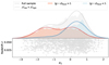 |
Fig. 1. Top: Ideogram of the stretch distribution for the full sample (in grey), and for SNe in locally red and blue environments (509 and 429 SNe). The full grey line is the bimodal Gaussian from N21 described in Sect. 3, while the red and blue lines are bimodal Gaussian fits to the old and young progenitor subpopulations. Bottom: Stretch vs redshift, z. The fact that there is no depletion of low stretch SNe at a higher redshift is a consequence of the volume-limited cut. |
3.1.1. Discussion on SN Ia stretch bimodality
This distribution is very similar to the one from the Nearby Supernova Factory (hereafter SNfactory, Aldering et al. 2002; Rigault et al. 2020) dataset studied in detail in Nicolas et al. (2021, hereafter N21). It is also similar to other nearby SN Ia data sets, like the one from Foundation (Foley et al. 2018) and the low-z Pantheon compilation (Scolnic et al. 2018), both studied in Fig. 6 of Popovic et al. (2021), or the Supercal compilation (Scolnic et al. 2015) studied in Fig. 3 of Wojtak et al. (2023). These latter samples do exhibit a bimodal distribution, but some with both modes equally populated, unlike what we observed with our volume-limited sample. This is likely caused by complex selection effects affecting those low-z samples (see discussion in N21). In contrast, higher redshift samples do not display a clear bimodal distribution. According to N21 and Rigault et al. (2020), this is to be expected. In their model, since low-stretch SNe Ia only originate from old environments and since the cosmic star formation strongly increases with redshift (Madau & Dickinson 2014; Tasca et al. 2015), the fraction of (supposedly) old progenitor SNe Ia is lower; consequently, the low-stretch mode tends to vanish with redshift.
We present in Table 1, the bimodal Gaussian distribution parameters estimated on the volume-limited ZTF data set, and the best fit distribution is shown in Fig. 1. The fitted model is defined as follows:  .
.
Our results are in good agreements with those reported by N21. To get the ratio of the two modes r for N21, we had to use the assumption made in Rigault et al. (2020); namely, at their redshift, the fraction of young and old progenitors is half-half. The stretch mode parameters are compatible at the ∼1σ level. The sole remarkable difference is that the amplitude of the r parameter seems lower in our data set, though only at a 1.9σ level. If confirmed, such a reduced amplitude of the high-stretch model could suggest that either the low-stretch mode is slightly more populated than the high-stretch one in the old (delayed) population or that the fraction of old population is slightly higher than the expected 50% modelled by Rigault et al. (2020) for our median redshift (zmedian = 0.044).
3.1.2. Stretch distribution in locally red or blue environments
We split the ZTF volume-limited SNe Ia as a function of their local environment to further investigate the origin of the observed bimodality. Following, for instance, Roman et al. (2018), Kelsey et al. (2023), Briday et al. (2021), Wiseman et al. (2022), we used the local (2 kpc-radius) colour (g − z)local, as it performs well as a proxy for the underlying SN Ia prompt and delayed subpopulations used in N21, with locally blue and red environments hosting young and old SN Ia progenitors. Splitting the ZTF data at (g − z)local = 1 mag, 54% of the SNe Ia are found in a locally red environments and 46% in a locally blue environment.
The stretch distribution per local environment and the best bimodal fit for each subgroup is shown in the top panel of Fig. 1. We have drawn three main conclusions from this figure. First, the locally red environment SNe Ia are consistent with being equally populated with each mode (r = 49 ± 9%). Second, the locally blue environment SNe Ia have a non-null low-stretch mode (7.5 ± 1.8%). This is consistent with N21 modelling, that assumes the low-stretch mode to only be accessible to old-population SNe Ia once the environmental contamination is accounted for. Indeed, according to Briday et al. (2021),  of the colour classifications are false, namely, old-progenitor SNe Ia are associated to blue environments and vice versa. Thus, we expected 8% of old-population SNe Ia to be classified as locally blue (see Fig. 3 of Briday et al. (2021)) and so, ∼4% of the locally blue sample to be in the low-stretch mode. Third, the mean of the high-stretch mode seems to slightly vary as a function of local environment, with
  . This is further discussed in the next section.
3.2. Correlation between SN stretch and SN environment
In this subsection, we investigate the correlation of stretch with environment, namely, the local colour (g − z) and global mass. We are able to disentangle their effects, with the proportion of SNe Ia in high and low stretch modes being dependent on local colour, while the dependence of the mean stretch is tied to global mass. This modelling is shown in Sect. 3.2.3.
3.2.1. Qualitative study of stretch environmental correlations
We show in Fig. 2 the connection between SN Ia light-curve stretch parameter, x1, and host galaxy mass as well as local environment colour. We clearly see that the low-stretch mode only exists in locally red environments and massive host galaxies. Both are connected, since these environmental parameters are highly correlated, as illustrated in Fig. 3. This is consistent with earlier findings that the low-stretch mode only exists in old stellar population progenitors (e.g. Hamuy et al. 1996; Howell et al. 2007; Rigault et al. 2020; Nicolas et al. 2021; Larison et al. 2024), as those strongly favour massive hosts and make the local environment redder.
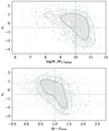 |
Fig. 2. Correlation between SN Ia light-curve stretch (x1) and host stellar mass (top), as well as the local environment colour (bottom). The contours show the area containing 97%, 84%, and 50% of the SNe Ia. Vertical lines show the environment splitting values, while the horizontal lines show x1 = −0.5, the typical transition point between stretch modes (see Fig. 1). |
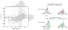 |
Fig. 3. Connections between SN Ia light-curve stretch (x1), global stellar mass (log(M*/M⊙)global), and local environmental colour ((g − z)local), illustrating the complex correlation between stretch and SN environmental properties. Left: Local colour vs global host stellar mass. The light grey band shows the 25%–75% percentile range for host global mass (vertical, [9.5, 10.5] dex) and local environmental colour (horizontal, [0.7, 1.3] mag). These cuts are used to select SNe Ia shown in the right panels. Top-right: Local environmental colour and SN stretch distributions for SNe Ia whose host global mass is in [9.5, 10.5] dex. Blue and red histograms show locally blue and red environment SNe Ia. The black histogram is the local colour distribution for the full sample. Bottom-right: Global host stellar mass and SN stretch distributions for SNe Ia whose local environmental colour is in [0.7, 1.3] mag. Purple and green histograms show low and high mass hosts SNe Ia. |
Figure 2 further shows that the connection between stretch and environment is more complex than the simple appearance of a low stretch mode in old-population environments as modelled, for instance, by Nicolas et al. (2021). There seems to be a correlation, clearly visible in the high-stretch mode, such that lower mass host and bluer environments tends to have a higher stretch. To investigate the origin of this effect, we look at the detailed connection between the SN light-curve stretch, global host mass, and local environmental colour in Fig. 3.
We split the data along the host stellar mass and local environment colour to investigate which of the environmental parameters is the most connected the our observations; namely, the appearance of the low-stretch mode and the stretch evolution. To do so, we only considered SNe Ia within the 25%-75% range of an environmental parameter (e.g. host stellar mass), and then study the correlation between x1 and the other environmental tracer (e.g. local colour), as shown on the top-right panels of Fig. 3. We see that the local colour distribution post host stellar mass 25%–75% selection is similar to that of the entire initial data set. Looking at the bottom-right panel of Fig. 3, we notice the same thing for the stellar mass distribution after the local-environmental 25%-75% selection. However, the resulting x1 distributions per environment are very informative on the origin of the two observed effect. For the given stellar mass range, locally red SNe Ia seem to have the same high-stretch mode and show in addition the apparition of the low-stretch mode (top-right panel). For a given local environmental colour range, the high- and low-mass host SNe Ia have a similar but shifted (Δx1 ∼ −0.5) x1 distributions (bottom-right panel).
From these observations, we conclude that the proportion of SNe in each stretch modes is directly connected to the local colour, while the apparent evolution of the mean stretch is connected to the global host stellar mass. The observed evolution of the high-stretch mode in the bottom panel of Fig. 2 thus seems to be a projection of the evolution connected to the global host stellar mass. Then, assuming that the light-curve stretch is an intrinsic SN Ia property, we interpret these observations as follows: the low-stretch mode is only accessible to old-population progenitors (delayed) as already suggested in the literature (Howell et al. 2007; Sullivan et al. 2010; Rigault et al. 2020; Nicolas et al. 2021), but the stretch evolution is likely connected to the progenitor metallicity, since the stellar mass and stellar metallicity are tightly correlated (Tremonti et al. 2004; Sánchez et al. 2017). This may be connected to literature observations that SN Ia stretch is directly linked to the progenitor mass or produced 56Ni mass (e.g. Dhawan et al. 2017; Scalzo et al. 2014, and references therein). The link with SN stretch and environment is also studied with the ZTF SN Ia sample using clusters (Ruppin et al. 2025) and voids (Aubert et al. 2025) as environment tracers.
3.2.2. Origin of the shifted stretch distribution between host redshift and SNID redshift SNe Ia
We present in Fig. 4 the SN Ia stretch distribution comparing SNe Ia having a host galaxy redshift (‘gal-z’) with those without, where the redhsift is extracted from the low resolution SN spectra from the spectral energy distribution machine (SEDm, Blagorodnova et al. 2018), either from SNID (Blondin & Tonry 2007) or from host emission lines (‘snid-z’, see Smith et al. 2025 for details).
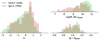 |
Fig. 4. SN Ia light-curve stretch (x1), global host mass (log(M*/M⊙)global), and local environmental colour ((g − z)local) distributions split per redshift origin. SNe Ia with galaxy redshifts are plotted in green (σz ∼ 10−4), and SNe Ia relying on low-resolution SN spectra (extracted from SEDm, Blagorodnova et al. 2018), either from SNID (Blondin & Tonry 2007) or on host emission lines are plotted in red (σz ∼ 10−3). The apparent stretch offset is explained by the selection function associated with galaxy redshifts, which favours high-mass hosts. |
We note that the stretch distribution for ‘gal-z’ SNe Ia is shifted by Δx1 ∼ 0.5 in comparison to that from ‘snid-z’ SNe Ia. This shift is explained by the selection function caused by our galaxy redshift sources (e.g. the (extended) Baryon Oscillation Spectroscopic Survey ((e)BOSS), see Smith et al. 2025), which strongly favours massive hosts, as illustrated in the top-right panel of Fig. 4. Interestingly, the local colour distributions are similar between these two SN samples. This further supports our claim that the stretch shift as a function of environment is driven by a physical mechanism more directly connected to global stellar mass than local colour, such as stellar metallicity (see details in Sect. 3.2.1).
3.2.3. Modelling of the stretch environmental dependencies
To quantify the observations described in Sect. 3.2.1, we extended the stretch model from N21 to account for the global mass dependency of the high and low stretch mode mean,  , described in the previous section and to get a more robust modelling of the relative fraction of high-stretch SNe Ia r as a function of the local colour. We denote (g − z)local ≡ cenv and log(M⋆/M⊙)global ≡ Menv for readability. The model is as follows:
 (1)
(1)
 (2)
(2)
with:
![Mathematical equation: $$ \begin{aligned} r(c_\mathrm{env} )&=r_\mathrm{red} + (r_\mathrm{blue} -r_\mathrm{red} )\times \mathcal{S} \left(\frac{1}{K_c}[c_\mathrm{env} -c_\mathrm{env} ^0]\right),\end{aligned} $$](/articles/aa/full_html/2025/03/aa50378-24/aa50378-24-eq10.gif) (3)
(3)
 (4)
(4)
In Eq. (2), 𝒮 is a sigmoid function, while rred and rblue correspond to the fraction of high-stretch mode SNe Ia in the blue and red ends of the environmental colour distribution, as illustrated in Fig. 5. We fit the data with this model accounting for errors on x1 and cenv (i.e. the local colour (g − z)local). The best fit parameters are displayed in Table 2. To quantify the improvement of this model over simpler versions, we compute AIC differences. Comparing the model of N21, where the transition between the young and old progenitors stretch distribution (blue and red distribution in Fig. 1) is sharp, with a model with a smooth transition (the sigmoid function plotted in Fig. 5), we found ΔAIC = 29, strongly favouring the smooth transition. We then compared this model to the full model, in which the means of the stretch modes evolves with mass, we get ΔAIC = 76. The addition of both a continuous dependence of the fraction of SNe Ia in the high-stretch mode on local colour and of the evolution of the means of the stretch modes with global mass is thus justified, as it is strongly supported by the data. The linear global mass dependency of the stretch modes (KM) is non-zero at the 9.2σ level, with KM = −0.30 ± 0.03 dex−1, strongly supporting the evidence that the means of the stretch modes are environment dependent.
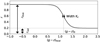 |
Fig. 5. Fraction of SNe in the high stretch mode as a function of the local colour, as modelled in Eq. (2). |
We also note that the apparition of the low-stretch mode is progressive, and the fraction of SNe Ia in the low-stretch mode only reaches its redder value of (1 − r)∼0.8 at (g − z)local ∼ 1.7 mag, as seen in Fig. 5. This behaviour is more complex than the sharp transition modelled in N21 and explains the ∼50% of low-stretch SNe Ia in red environments seen in Fig. 1.
4. Stretch-residuals relation
In this section, we study the SN Ia stretch standardisation procedure accounting for the brighter-slower Phillips (1993) relation. We briefly introduce SN Ia standardisation in Sect. 4.1 and present our fitting procedure in Sect. 4.2, as well as the resulting standardisation parameters in Sect. 4.3. We then assess the universality of this procedure as a function of SN environment in Sect. 4.4, to finally question its assumed linearity in Sect. 4.5. The colour standardisation is studied in detail in a companion paper (Ginolin et al. 2025).
4.1. SNe Ia standardisation
We define the difference between observed and modelled distance moduli, also called Hubble residuals, as:
 (5)
(5)
where μcosmo is calculated in astropy (Astropy Collaboration 2013, 2018), following a flat ΛCDM cosmology given by Planck Collaboration VI (2020, Ωm = 0.315), plus a blinded magnitude offset. We then use Chauvenet’s criterion to reject outliers of the cosmological fit, which discards 7 SNe.
The usual standardisation formula for SNe Ia is given by:
 (6)
(6)
 (7)
(7)
where M0 is the absolute B-band SN magnitude (degenerate with H0), α and β are the linear standardisation coefficients correcting for the stretch (x1) and colour (c) SN Ia variations following the slower-brighter and bluer-brighter relations (Tripp 1998). The γp term accounts for SN Ia magnitude environmental dependencies (e.g. Kelly et al. 2010; Sullivan et al. 2010; Briday et al. 2021). p is the probability that an environmental tracer m is below a given splitting value (‘cut’, see Table. 3), while γ is the magnitude offset between the SN Ia subpopulations below or above the environment cut, known as the ‘step’. In practice, p (∈[0, 1]) is the cumulative distribution function of the environmental proxy m measured with an error δm evaluated at the cut value, such that p = ∫−∞cut𝒩(x, m, δm)dx. In recent cosmological analyses, m is usually the global host stellar mass and γ is referred to as the mass step.
Stretch correction coefficient (α) and absolute magnitude (M0) as a function of the SN environment.
The Δb term accounts for selection function affecting the survey, since overly bright objects are easier to acquire and to classify. The correct modelling procedure of this term is highly discussed, and has been shown to bias the environmental correction if not accurately done (e.g. Smith et al. 2020; Popovic et al. 2021; Nicolas et al. 2021; Wiseman et al. 2022). In this analysis, to avoid such complications, we use the volume-limited sample of the ZTF DR2 sample (z < 0.06), which is free from non-random selection functions either from light-curve estimation or spectral typing (Smith et al. 2025; Amenouche et al. 2025). Consequently, we set Δb = 0.
The standardisation (i.e. estimation of M0, α, β, γ; see. Eq. (5)) was done using total-χ2 minimisation. The total-χ2 approach enables to fit a model explaining an observed y-variable (here, Δμ) that depends on input noisy x-variables (here c, and x1, p). Unlike a simple χ2 minimisation, this requires fitting for the true (noisy) x-variables that are used, in turn, to estimate y.
4.2. Total-χ2 minimisation.
In practice, for a sample containing N SNe, we fit for 3 × N + 5 parameters: the 3 × N parameters corresponding to the true values of the observed noisy standardisation variables (ctrue, x1true, and ptrue), the four standardisation parameters of interest from Eq. (5) (α, β, γ and M0), plus an intrinsic magnitude scatter σint to account for leftover dispersion in the residuals.
The ‘total’ χ2 is thus the sum of two parts, one quantifying the likelihood that the observed x correspond to the fitted xtrue:
 (8)
(8)
and the usual χ2 standardisation, computed with the ‘true’ x-variables:
 (9)
(9)
where  , and ℂi is the covariance matrix between (μi, x1i, ci). Hence, including the determinant logdet = ∑ilog(σobsi2 + σint2), we minimise χ2 = χres2 + χparam2 + logdet.
In our fit, we consider p as non-noisy as it already takes into account errors on the environment parameter chosen to compute the magnitude step, so we assign it arbitrarily small errors σp, such that ptrue is effectively equal to p. To avoid biases, the intrinsic scatter is fitted iteratively. We fix a given σint, find the parameters (α, β, γ, M0, (x1true)i, (ctrue)i) that minimise the total-χ2, then fix those parameters and fit σint as the value that normalises the reduced total-χ2. This procedure is repeated ten times. The error estimation on the parameters is then done at fixed σint using a 1000 steps of a Markov chain Monte Carlo (MCMC) algorithm. Finally, the corrected residuals are computed using the measured c, x1, and p.
Based on realistic simulations, we show in Appendix A that this fitting approach is unbiased, unlike the simple χ2 approach, which assumes xobs = xtrue. For a wide range of α, β, γ, and σint combinations, we recovered the input parameters and accurately estimate their errors, as our residual pulls (difference between the fitted and input parameter divided by the fitted error) follow a Gaussian distribution (centred on 0 with a width of 1).
This fitting procedure makes use of jax (Bradbury et al. 2018). Additional details on the use of total-χ2 for cosmological parameter inference in SN cosmology will be given by Kuhn et al. (in prep.).
4.3. Standardisation parameter coefficients
Fitting on our 938 SNe Ia sample with the total-χ2 procedure described in Sect. 4.2, we find α = 0.161 ± 0.010, β = 3.05 ± 0.06 and γ = 0.143 ± 0.025 using local colour as our environmental tracer (e.g. Roman et al. 2018; Kelsey et al. 2021; Briday et al. 2021). σint is not released, as it will be the subject of a future detailed analysis.
The correlation matrix of the fitted (β, α, M0, γ) is plotted in Fig. 6. We see a strong correlation between the stretch standardisation parameter α and the environmental step γ. This is expected, as γ traces the magnitude bias due to environment and stretch is strongly linked with environment, as seen in Sect. 3. Because of the correlation between α, β and γ, it is necessary to fit them jointly. Indeed, fitting for only α and β and computing γ as an a posteriori difference between the Hubble residuals for SNe in different environments will lead to α and β absorbing part of the magnitude-environment connection. This will in turn bias α and β, and underestimate the step γ. This is discussed in more details in Sect. 5.
As illustrated in Fig. 7, the Hubble residuals are normally scattered, with a width (normalised median absolute deviation, nmad) of 0.175 mag. The regular STD of the Hubble residuals is 0.226 mag. Discarding SNe Ia that have redshift extracted from SN Ia spectroscopic features (25% of the sample, hence leaving 707/945 SNe Ia) leads to very similar results (α = 0.173 ± 0.009, β = 3.06 ± 0.05 and γ = 0.143 ± 0.022), but with a reduced nmad of 0.16 mag (0.213 for the regular STD). This reduction is expected since SN Ia-features redshift having a typical precision of 3 × 10⁻³ (see details in Smith et al. 2025), corresponding to an additional 0.08 mag scatter, to be added in quadrature. The amplitude of the step γ is discussed in Sect. 5, β is studied in a companion paper (Ginolin et al. 2025) and α is further discussed in the following subsections.
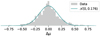 |
Fig. 7. Histogram of the standardised Hubble residuals (corrected for SN colour, SN stretch, and environment). The blue line is a Gaussian centred on 0 with a standard deviation corresponding to the normalised median absolute deviation σnmad = 0.176. |
4.4. Environmental dependency of the stretch standardisation
The universality of the brighter-slower and brighter-bluer empirical linear relations might be challenged by observed environmental dependencies of such standardised SN Ia magnitudes, for instance, the mass-step (e.g. Sullivan et al. 2010), the local colour bias (e.g. Roman et al. 2018), or the age bias (Rigault et al. 2020), which most likely are different aspects of the same underlying effect (e.g. Briday et al. 2021; Brout & Scolnic 2021).
In this subsection, we explain how we tested whether the stretch standardisation coefficient, α, itself is environment dependent. Using the environmental tracers introduced in Sect. 2.2, we split our volume-limited sample in two, following the cuts introduced in that section (see also Table 3). For each of these four environmental tracers, we independently standardise the two SN subsamples. We report in Table 3 the recovered stretch (α) and absolute magnitude (M0) parameters. The colour term (β) is discussed in a dedicated paper (Ginolin et al. 2025). The M0 offset, equivalent to the step, is discussed in Sect. 5.
We see in Table 3 that the stretch standardisation parameter α does not seem to strongly depend on the environment. The most significant difference appears when using global host mass as tracer, with Δα ∼ −0.06 at the 3.0σ level, such that high-mass galaxies host SNe Ia with a larger α coefficient. This is consistent with earlier findings that the standardisation coefficients do not seem to depend on environment given the small data sets these analyses had access to (e.g. Sullivan et al. 2010; Rigault et al. 2020; Kelsey et al. 2021). The small dependence of α on environment is actually the signature of the non-linearity of the stretch-residuals relation, studied in detail in Sects. 4.5 and 6.4.
4.5. Linearity of the stretch-magnitude relation
The next standardisation assumption we challenge is the linearity of stretch-residuals relation (see e.g. Fig. 8 of Sullivan et al. 2011; Wang et al. 2006; Rubin et al. 2015). More recently Garnavich et al. (2023), Larison et al. (2024) presented 3 to 4.5σ evidence for different α coefficients as a function of SN stretch, using 𝒪(100) SNe Ia.
We illustrate in Fig. 8 the stretch standardisation step for our sample. This figure shows the Hubble residuals standardised for colour and environment, but not for stretch, as a function of stretch (x1). This relation was assumed to be linear by all SN cosmological analyses so far (e.g. Riess et al. 1998; Perlmutter et al. 1999; Betoule et al. 2014; Scolnic et al. 2018; Brout et al. 2022). Yet, it is visible in Fig. 8 that the stretch-residuals relation is not linear, as suggested by Garnavich et al. (2023), Larison et al. (2024). It indeed has a distinct broken shape, with lower-stretch SNe Ia having a stronger (in absolute value) α coefficient than high-stretch SNe Ia. Hints of this behaviour are also seen in the ZTF SN Ia DR2 siblings (Dhawan et al. 2024) and host-morphology (Senzel et al. 2025) studies.
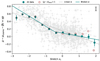 |
Fig. 8. Standardised Hubble residuals (α = 0) as a function of stretch (x1). Large blue points show the data binned by stretch (mean) while the red hexagons show the binned stretch for SNe Ia from locally red environments. The errorbars on the binned points only display the error on the mean, but a reference for the fitted intrinsic scatter σint is plotted in the top-right corner. The blue line shows the best fitted broken-α model, while the dashed grey line shows the best α when assuming the linear Tripp relation. |
To quantify this observation, we update Eq. (4.1) to allow for a broken-α standardisation. This introduces two extra parameters αlow and αhigh, in place of a single α, and the breaking point x10, which is also fitted:
 (10)
(10)
with
 (11)
(11)
In fitting this ‘broken line’ model, we find αlow = 0.271 ± 0.011 and αhigh = 0.083 ± 0.009. The two α significantly differ at the 13.4σ level, with Δα = αhigh − αlow = −0.188 ± 0.014. Such a high-significance demonstrates that indeed, the stretch-residuals relation is non-linear. We also find a reduction of the fitted intrinsic scatter (−40%). The reduction of the scatter indicates that the broken-α absorbs some of the unexplained scatter dubbed as intrinsic. While fitting for a broken-α, we find βbroken = 3.31 ± 0.03. A detailed study of the intrinsic scatter will be the subject of a dedicated analysis and the actual σint values are thus not published.
The evaluation of the improvement of the fit by adding two extra parameters is not straightforward, as the χ2 of the fit depends on σint, as explained in Sect. 4.1, which differs in the linear and broken-α case. If we fix σint to the broken-α value, we find ΔAIC = 101. When assuming the larger σint associated to the linear-α model, we find ΔAIC = 48, with the significance of the broken-α being reduced to 6.2σ. In both cases, the broken-α model is favoured by the data.
We highlight that such a broken-α result is very unlikely to be caused by an unknown selection function. Indeed, this would cause to miss objects preferentially in the top-left corner of Fig. 8 (faster and fainter objects), which would in turn pull αhigh to lower values. The robustness of this result is further demonstrated in Sect. 6.1.
The best-fit value of the stretch split x10 is also of interest. When fitting the broken-α model with a variable breaking point, we find x10 = −0.48 ± 0.08, which corresponds to the transition between the two stretch modes visible in the x1 distribution in Fig. 1. This may suggest that there is a physical difference between the two stretch modes, resulting in the different stretch-residuals correlation. With the current modelling used, both modes share the same absolute standardised magnitude at the breaking point, hinting at a continuous transition between the two modes. This would need to be further investigated in a dedicated modelling analysis. Additionally, we investigate in Sect. 6.2 the dependence of the broken-α on SN colour.
4.6. Environmental dependency of the stretch-magnitude relation non-linearity
In Fig. 8, we plot the binned environment-standardised SN Hubble residuals as a function of stretch for locally red environment SNe Ia only ((g − z)local > 1). Unlike the blue (younger) environments, these SNe Ia populate both stretch modes (see Sect. 3), which enables us to test whether the broken relation is indeed driven by the SN Ia stretch mode (it should thus also be there for red-environment SNe Ia) or if it is an artifact of an environmentally dependent α (the magnitude-stretch relation should then be linear). Considering only red-environment SN Ia, we find Δα = −0.255 ± 0.048 (5.3σ), demonstrating that the broken-α effect is not caused by an environment-dependent α; rather, it is rather a stretch-mode driven effect, with each stretch modes having their own stretch-magnitude relation. We reached the same conclusion when fitting a broken-α on SNe Ia in high-mass hosts, with Δα = −0.204 ± 0.043 (4.8σ). Since the relative fraction of each mode is strongly environment-dependent (see Sect. 3), this non-linearity leads to variation of the usual α standardisation as a function of the environment and redshift (see dedicated discussion in Sect. 6.4).
5. SN Ia standardised magnitudes (steps)
In this section, we investigate the amplitude of the environmental magnitude offsets affecting our volume-limited sample. These offsets between SN environments, aka steps, are represented by the γ term in Eq. (5) and computed simultaneously with the other standardisation parameters. We illustrate in Fig. 9 the local colour step, manually setting γ = 0 to get Hubble residuals uncorrected for environment. This figure clearly demonstrates the existence of astrophysical biases affecting stretch and colour standardised SN Ia magnitudes. Indeed, SNe Ia in locally blue environments are significantly fainter (γ = 0.143 ± 0.025 mag) than those from locally red environments. Accounting for the non-linearity of the stretch-residuals relation, we find γ = 0.175 ± 0.010 mag.
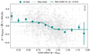 |
Fig. 9. Standardised Hubble residuals corrected for stretch (with a broken-α) and colour as a function of local environmental colour. Large blue points show the residuals binned by local colour, with the errorbars corresponding to the error on the mean. The scale of the fitted intrinsic scatter is shown in the top-right corner. The dashed line shows the step model. The full line illustrates the step model once convolved by a Gaussian with a standard dispersion equals to the mean local environmental measurement error (σ(g − z),local ∼ 0.14), as we account for those errors in the step model. |
Nonetheless, the actual origin of the observed astrophysical bias is still highly debated, and Brout & Scolnic (2021), Popovic et al. (2021) suggest that the mass step originates from different dusts properties for different environments (see further discussion in Kelsey et al. 2023; Wiseman et al. 2022). Modelling dust with BayeSN (Thorp et al. 2021; Mandel et al. 2022), Grayling et al. (2024) find an intrinsic mass step of −0.049 ± 0.016 mag. Finally, Smith et al. (2020) show that selection function corrections inaccuracy affects the ability to measure environmental biases, since all parameters are correlated (e.g. stretch, colour, host mass, local colour). The strength of our volume-limited data set is that we are free from such selection issues.
The fact that the steps, derived from a low-redshift volume-limited dataset, are found to be significantly larger than those from higher-redshift samples may be due to two things. First, the amplitude of the mass step may decrease with redshift (Rigault et al. 2013, 2020; Childress et al. 2014). Second, as the effect of selection function and the dependencies of SNe Ia with their astrophysical environment are intertwined, bias corrections, which are necessary at high-redshift, might affect the derivation of the step. We note that the amplitude of our step is compatible with the value found by Rigault et al. (2020) using another low-redshift, volume-limited sample (SNfactory, Aldering et al. 2002).
The amplitude of the step is connected to the ability to accurately perform stretch and colour standardisation, since SN stretch (mostly) and colour are correlated with environmental parameters (see Fig. 2 for the stretch-local colour connection). Hence, as already discussed in Smith et al. (2020), Dixon (2021), Briday et al. (2021), when fitting first for α and β, and then for γ (as e.g. in Kim et al. 2019 for a recent example), the colour and stretch standardisation will absorb part of the (ignored) astrophysical biases, thus biasing all terms (α, β and γ ; see, e.g. discussion in Rigault et al. 2020; Smith et al. 2020; Dixon 2021; Briday et al. 2021). Such ‘a posteriori’ measurements can then only underestimate the step.
The best fitted γ parameters are presented in Fig. 10 and reported in Table 4. For comparison, the figure also includes the ‘a posteriori’ step results, as well as the ΔM0 offset acquired when applying a per-environment standardisation and the steps obtained using a broken-α relation (see Sect. 4.5).
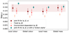 |
Fig. 10. Fitted steps for each of the environmental proxies. The dark red and green points indicate steps where both (α, β) and γ are fitted at the same time for each proxy. The light red points indicate the steps when the same (α, β) correction (fixed across proxies) is applied to the whole sample. The red points indicate the steps when independent (α, β) corrections are applied for each of the subsamples. The green points are steps when including the broken-α model into the fit, according to Sect. 4.5. The shaded band represents the 1σ interval for the reference step (local colour step from the joint fit). |
Amplitude of the environment magnitude offset, aka steps, for the joint fit for (α, β, γ), without and with broken-α.
All of magnitude offsets in Table 4 are significantly non-zero at the ≥5σ level. When using the usual Tripp (1998) linear standardisation formalism, the strongest one is the global mass step with γ = 0.145 ± 0.021 mag (6.8σ). The local colour step is at a similar level, in agreement with Roman et al. (2018), Kelsey et al. (2021), and Briday et al. (2021). The amplitude of the global mass step is consistent with findings reported in SNfactory (Rigault et al. 2020), but higher than the steps reported in SDSS/SNLS (Roman et al. 2018) and DESY3 (Kelsey et al. 2021).
As expected, Fig. 10 shows that the environmental steps derived after standardisation are significantly biased towards smaller values, with a reduction of ∼0.05 mag. When comparing the amplitude of magnitude offsets when the standardisation is made independently for the two environments, all steps remain strongly significant (> 5σ level), demonstrating that environmental inhomogeneity of the standardisation procedure is not responsible for SN magnitude biases, as already suggested in Sect. 4.4. Furthermore, accounting for the non-linearity of the stretch-magnitude relation (see Sect. 4.5) slightly increases the amplitude of all the environmental steps and reduce the parameter errors, see Fig. 10. This is to be expected if indeed the non-linearity is true, since the fitted model is more representative of the data, and thus all parameters are better measured. This also demonstrates that the existence of two stretch modes having each their own α term is not responsible for the environmental magnitude offsets. Altogether, local tracers perform slightly better than global ones when using the broken-α standardisation.
To ensure that the discrepancies between the step values are indeed due to variations in the fitting procedure, we investigated the differences between these step fitting methods using simulations in Appendix A.3. We reproduce both the order of the points and the factor between the jointly fitted step (red points) and the a posteriori step (light red points) for the local colour step. This confirms that not performing a joint fit for the environmental step along with α and β will underestimate it.
6. Discussion
6.1. Robustness tests
In this section, we explain how we tested the robustness of our main results, namely the evolution of the stretch modes with global mass (KM parameter from Eq. (3)), the non-linearity of the stretch-residuals relation and the amplitude of the magnitude steps, by applying several analysis variations:
-
Varying the redshift cut we used to define our volume limited sample, reducing it to zmax = 0.05 as a conservative cut, we were able to test whether our results could be caused by a leftover selection function. We also extended our analyses to zmax = 0.07, to gain statistical power, with a limited Malmquist bias.
-
Only using SNe Ia with host redshifts, whose residual scatter is smaller.
-
Changing the SN Ia subpopulations used in the study. We include the subluminous 91bg population as well as SNe Ia classified as peculiar, as these could be hard to identify in higher redshift surveys for instance, or in surveys relying on photo-typing. We also redo the analysis discarding 91t. This allows us to test that our results are not driven by the 91t subpopulation.
-
Using the literature cut on SN colour (c < 0.3) to make sure our results are not affected by the inclusion of red objects.
-
Applying a much stronger cut on light-curve fit probability (χSALT2 < 0.1), to check if our results could be induced by ill-modelled light-curves.
The result of all these variations are summarised in Table 5.
We see no significant variations across all the modifications we made. Accessing an even more secured volume-limited sample only slightly reduces the significance of our results, as we reduce our statistics, strengthening our claim that the broken-α or the step amplitudes are not caused by any uncontrolled selection effect leftover. Going up to zmax = 0.07 does not changes our results, which might hint that the volume-limited cut we made is conservative. Only using host redshifts reduces the significance of the evolution of stretch with global mass. This is expected, as the host redshift sample is biased towards higher mass hosts (see Sect. 3), thereby reducing the leverage of the fit. The significance of the broken-α also decreases, due to the reduced statistics. Adding the peculiar 91bg-like objects, discarding 91t from our sample or only using c < 0.3 SNe does not impact the significance of our results. The significance of the broken-α decreases slightly when discarding c > 0.3 objects, but it is still higher than the 10σ level. This confirms that red SNe do not exhibit peculiar behaviour, confirming the conclusions of Rose et al. (2022) and Ginolin et al. (2025). Enforcing a strong light-curve fit requirement also has only a slight impact on KM and Δα, due to lower statistics, confirming that it is not a light-curve modelling issue that may cause either the broken stretch-residuals relation or the observed astrophysical bias (see a dedicated light-curve residual analysis in Rigault et al. 2025b).
6.2. Dependence of the broken-α on SN colour
As an additional test of the broken-α, we looked at its value when cutting the sample into red (c > 0, 559 SNe) and blue (c < 0, 379 SNe) SNe. We show in Fig. 11 the residuals corrected for colour and environment against stretch. The broken-α is still visible for both subsamples. We find Δα to be respectively 8.5σ and 5.1σ away from 0 for the red and blue sub-samples. The reduction of the significance is expected due to the lower number of SNe in each sub-sample. We thus conclude that the non-linearity of the stretch-residuals relation does not depend on SN colour.
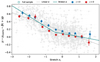 |
Fig. 11. Hubble residuals corrected for colour and environment as a function of stretch x1 (same as Fig. 8), for the full sample (white points) and blue and red SNe (blue and red points). |
We note in Fig. 11 that the blue SNe Ia residuals are ∼0.07 mag fainter than the red SNe Ia ones. As detailed in Appendix A of Ginolin et al. (2025), this offset is caused by measurement noise in colour, that creates an up-tail towards blue values on correctly standardised Hubble residuals. We highlight that this is not a signature of a non-linearity in β; as explained in Sect. 4.1 of Ginolin et al. (2025), which confirms that the colour-residuals relation is linear.
6.3. Pocket effect
As discussed in Sect. 2, the ‘pocket effect’ that appeared in some of the ZTF CCDs after October 2019 can impact stretch measurements (Lacroix et al. (in prep.), Rigault et al. 2025a), leading to an overall shift in stretch of Δx1 ∼ −0.1 for these SNe Ia. In this section, we investigate the impact of this effect on our results by cutting our sample in two: SNe with t0 before 1 October 2019 (451 SNe Ia), which were unaffected by the pocket effect, and those with t0 after December 2019 (420 SNe Ia). SNe Ia at peak in October and November are discarded, as their light-curves were only partially affected.
We first checked that our data have indeed been impacted by a stretch shift. Thus, we refit the double Gaussian stretch model presented in Sect. 3.1, but allowing for a shift between the two samples. The recovered parameters of the double Gaussian are similar to those from the full sample (within 1σ) and the fitted shift is Δx1 = −0.1 ± 0.06, in agreement with simulations.
To check that our main results were unaffected by the pocket effect, we report in Table 5 the values of the evolution of the stretch modes with host mass, the significance of the broken-α, and the environmental steps for SNe Ia before and after the pocket effect, as done in Sect. 6.1.
We first look at the dependency of the stretch mode means with the host stellar mass, parametrised by KM. The significance of KM is reduced from 9σ (full sample) to ∼6σ for SNe Ia from both subsamples. Such a lower significance is expected given the reduction of the sample size. Indeed, randomly drawing 450 SNe Ia from the full sample and carrying out a refitting for KM leads to a 6σ or lower signal 36% of the time. Moreover, the values of KM are similar between subsamples (KM = −0.33 ± 0.05 for SNe Ia after Dec. 2019 and KM = −0.24 ± 0.04 for SNe Ia before Oct. 2019), and similar to the value for the full sample (KM = −0.30 ± 0.03).
The amplitude of the broken-α shows the strongest variation between the two samples: 7.3σ for the 451 SNe Ia unaffected by the pocket effect and 11.8σ for the 420 SNe Ia impacted by it. It thus raises the question if this difference is simple causes for a reduction of the sample size. To evaluate this, we randomly select 450 SNe Ia from the full sample and fit for a broken-α. Carrying out this process 1000 times, we find 22% of the downsized sample have Δα < 7.3σ (96% of 11.8σ of less). Furthermore, the values of Δα are compatible between subsamples: for the SNe Ia before Oct. 2019, we find αlow = 0.257 ± 0.014 and αhigh = 0.131 ± 0.010, while for the SNe Ia after Dec. 2019 we find αlow = 0.300 ± 0.014 and αhigh = 0.086 ± 0.011. We thus conclude that the pocket effect does not significantly impact the broken-α.
We finally investigated the environmental step amplitudes. The steps are similar between samples (less than a ∼1.5σ difference), both for the linear and broken-α standardisation. We thus conclude that the pocket effect has no significant impact on the amplitude of the steps reported in this paper.
6.4. Broken α and linear standardisation biases
As presented in Sect. 4.5, the Phillips (1993) stretch-residuals relation, parametrised by the α term in Eq. (5), is non-linear. This non-linearity coincides with the light-curve stretch bimodality (see Fig. 1 and e.g. N21), such that high-stretch mode SNe Ia have a weaker stretch-residuals correlation (αhigh ∼ 0.08) than those from the low-stretch mode (αlow ∼ 0.27; see Fig. 1 and dedicated discussion in Sect. 4.5). Yet, the low-stretch mode is only accessible to SNe Ia from old population environments (see Sect. 3.1.2 and e.g. Howell et al. 2007, Sullivan et al. 2010, Rigault et al. 2020, Nicolas et al. 2021), unlike the high-stretch mode, which is always available. Since the fraction of old-population SNe Ia varies with redshift and/or with environment, the use of a (usual) linear standardisation parameter α will lead to variations of α with redshift and environment. This is particularly important in two cases, redshift evolution and selection bias.
Here, we carry out a qualitative evaluation of the effect of fitting a linear α if the truth is a broken α. A more thorough investigation of this problem, along with simulations, will be presented in a future paper.
Following Rigault et al. (2020), the fraction of SNe Ia from young progenitors increases with redshift, going to almost 1 at z ∼ 2. As they only populate the high-stretch mode, which has αhigh ∼ 0.08, a linear α will evolve from its main sample value (α ∼ 0.16) to a value close to αhigh when going to higher redshifts. We thus predict a decrease of a linear α with redshift.
Following the same reasoning, as low-strech SN Ia are fainter, lowering the magnitude limit of a survey thus increases the fraction of SNe Ia in the high-stretch mode, and biases a linear α towards αhigh. We thus predict a decrease of a linear α when discarding objects due to a magnitude limit. Additionally, as shown in Sect. 3, stretch is strongly correlated with environment. Indeed, SNe Ia in locally blue environments and/or low mass hosts only have access to the high-stretch mode. Hence, selecting SNe Ia only in those environments would bias a linear α towards αhigh (and towards αlow for locally red environments and/or high mass hosts). Yet, to maximise the acquired SNe Ia rate, it is common for SN Ia samples to be biased towards a given environment (e.g. mid-mass blue spiral galaxies), where it is easier to get a host redshift, as well as towards massive galaxies, as it is easier to get a host mass, or targeted surveys that only observe massive spirals. The effect of magnitude and environment are likely to add up, making disentangling their contributions even harder. This calls for caution when fitting a linear stretch-residuals standardisation, especially for non-volume-limited surveys. A more qualitative study of these effects, as well as the impact on the resulting fitted cosmology, will be presented in a upcoming analysis.
7. Conclusion
This paper presents a detailed analysis of the SN Ia standardisation procedure, focusing on the stretch (x1) residuals relation and SN environment magnitude offsets, aka steps. The companion paper Ginolin et al. (2025) focuses on SN colour. This analysis is based on the volume-limited data set (z < 0.06) of ∼1000 SN Ia from the SN Ia ZTF DR2 sample (Rigault et al. 2025a; Smith et al. 2025). This data set is free from significant selection function and therefore observed distributions, correlations and biases are representative of the true underlying SN Ia nature. Our conclusions are as follows:
-
The stretch-residuals relation, represented by the α term in the SN Ia standardisation (Tripp 1998), is non-linear. Low-stretch SNe Ia (x1 ≤ −0.48) have a much stronger magnitude-stretch relation with αlow = 0.271 ± 0.011 than high-stretch mode SNe Ia αhigh = 0.083 ± 0.009. This non-linearity is measured at the 13.4σ level.
-
The environmental dependency of standardised SN Ia magnitude is stronger than usually claimed. Accounting for the stretch-residuals non-linearity we find γ = 0.175 ± 0.010 mag using the local (2 kpc) colour (g − z) tracer, a 18.4σ detection. Even with a usual linear α (Tripp 1998) relation, we find γ = 0.143 ± 0.025 mag (a 5.6σ detection).
-
The global mass step is at a similar level than the local environmental colour step, with γ = 0.145 ± 0.021 mag (0.153 ± 0.013 mag, using a broken-α).
-
The stretch distribution is bimodal with mode parameters measured in close agreement with those derived by Nicolas et al. (2021). The low-stretch mode (x1 ≤ −0.5) is only available to SNe Ia from old-population environments (redder galaxies and/or more massive host), unlike the high-stretch mode.
-
The stretch modes means decrease linearly as a function of global host stellar mass (at a 9.2σ significance). We show that this, in turn, causes an apparent evolution of the stretch mode with local colour. This change is likely caused by the progenitor metallicity, that more directly correlates with stellar mass than with local environmental colour.
-
The complex stretch-environment connection can be summarised as follows: SNe Ia have two stretch modes, each having their own α. The low stretch mode is only available to SNe Ia from old-population environments (i.e. to ‘delayed’ SNe Ia). The mean of the x1 distribution slowly evolves as a function of host stellar mass, suggesting that SN metallicity influences x1, such that higher metallicity (more massive host) leads to SNe Ia with smaller stretch.
-
7
Because the stretch distribution evolves with redshift and as a function of environment, we expect that the Tripp (1998) linear α term should decrease as a function of redshift. This should also strongly vary as a function of selection effect, such as the magnitude limit or those favouring for instance blue emission line galaxies and/or mass hosts.
This analysis of the ZTF volume-limited sample has revealed unexpected SN Ia behaviours, notably the strong non-linearity of the SN Ia standardisation procedure. This would likely not have been possible without the combination of a large sample statistic and the fact that our sample is not significantly affected by any (potentially hard to model) selection function effects. As such, we are able to predict what such effects could cause on the derivation of the SN Ia standardisation parameters that, in turn, leads to the inference of cosmological parameters. Our well controlled sample also reveals large environmental SN magnitude offsets. Altogether, those astrophysical biases, induced by our limited understanding of what SNe Ia truly are, are a dominating source of systematic uncertainties, along with photometric calibration. To mitigate them, we strongly recommend for future surveys such as the Legacy Survey of Space and Time (LSST) and the Nancy Grace Roman Space Telescope to dedicate a fraction of their observing time to build a volume-limited SN Ia data set covering as much of the SN parameter phase space as possible. This is particularly true for the redshift component, as issues related to redshift dependencies directly translate to biases on the derivation of cosmological parameters.
Acknowledgments
Based on observations obtained with the Samuel Oschin Telescope 48-inch and the 60-inch Telescope at the Palomar Observatory as part of the Zwicky Transient Facility project. ZTF is supported by the National Science Foundation under Grants No. AST-1440341 and AST-2034437 and a collaboration including current partners Caltech, IPAC, the Weizmann Institute of Science, the Oskar Klein Center at Stockholm University, the University of Maryland, Deutsches Elektronen-Synchrotron and Humboldt University, the TANGO Consortium of Taiwan, the University of Wisconsin at Milwaukee, Trinity College Dublin, Lawrence Livermore National Laboratories, IN2P3, University of Warwick, Ruhr University Bochum, Northwestern University and former partners the University of Washington, Los Alamos National Laboratories, and Lawrence Berkeley National Laboratories. Operations are conducted by COO, IPAC, and UW. SED Machine is based upon work supported by the National Science Foundation under Grant No. 1106171 The ZTF forced-photometry service was funded under the Heising-Simons Foundation grant #12540303 (PI: Graham). This project has received funding from the European Research Council (ERC) under the European Union’s Horizon 2020 research and innovation program (grant agreement n 759194 - USNAC). MMK acknowledges generous support from the David and Lucille Packard Foundation. UB, MD, GD, KM and JHT are supported by the H2020 European Research Council grant no. 758638. LG acknowledges financial support from the Spanish Ministerio de Ciencia e Innovación (MCIN) and the Agencia Estatal de Investigación (AEI) 10.13039/501100011033 under the PID2020-115253GA-I00 HOSTFLOWS project, from Centro Superior de Investigaciones Científicas (CSIC) under the PIE project 20215AT016 and the program Unidad de Excelencia María de Maeztu CEX2020-001058-M, and from the Departament de Recerca i Universitats de la Generalitat de Catalunya through the 2021-SGR-01270 grant. This work has been supported by the research project grant “Understanding the Dynamic Universe” funded by the Knut and Alice Wallenberg Foundation under Dnr KAW 2018.0067, Vetenskapsrådet, the Swedish Research Council, project 2020-03444 and the G.R.E.A.T research environment, project number 2016-06012. YLK has received funding from the Science and Technology Facilities Council [grant number ST/V000713/1]. This work has been supported by the Agence Nationale de la Recherche of the French government through the program ANR-21-CE31-0016-03. TEMB acknowledges financial support from the Spanish Ministerio de Ciencia e Innovación (MCIN), the Agencia Estatal de Investigación (AEI) 10.13039/501100011033, and the European Union Next Generation EU/PRTR funds under the 2021 Juan de la Cierva program FJC2021-047124-I and the PID2020-115253GA-I00 HOSTFLOWS project, from Centro Superior de Investigaciones Científicas (CSIC) under the PIE project 20215AT016, and the program Unidad de Excelencia María de Maeztu CEX2020-001058-M. LH is funded by the Irish Research Council under grant number GOIPG/2020/1387. SD acknowledges support from the Marie Curie Individual Fellowship under grant ID 890695 and a Junior Research Fellowship at Lucy Cavendish College.
References
- Aldering, G., Adam, G., Antilogus, P., et al. 2002, in Survey and Other Telescope Technologies and Discoveries, eds. J. A. Tyson, & S. Wolff, SPIE Conf. Ser., 4836, 61 [NASA ADS] [CrossRef] [Google Scholar]
- Amenouche, M., Smith, M., Rosnet, P., et al. 2025, A&A, 694, A3 (ZTF DR2 SI) [NASA ADS] [CrossRef] [EDP Sciences] [Google Scholar]
- Astropy Collaboration (Robitaille, T. P., et al.) 2013, A&A, 558, A33 [NASA ADS] [CrossRef] [EDP Sciences] [Google Scholar]
- Astropy Collaboration (Price-Whelan, A. M., et al.) 2018, AJ, 156, 123 [Google Scholar]
- Aubert, M., Rosnet, P., Popovic, B., et al. 2025, A&A, 694, A7 (ZTF DR2 SI) [NASA ADS] [CrossRef] [EDP Sciences] [Google Scholar]
- Bellm, E. C., Kulkarni, S. R., Graham, M. J., et al. 2019, PASP, 131, 018002 [Google Scholar]
- Betoule, M., Kessler, R., Guy, J., et al. 2014, A&A, 568, A22 [NASA ADS] [CrossRef] [EDP Sciences] [Google Scholar]
- Blagorodnova, N., Neill, J. D., Walters, R., et al. 2018, PASP, 130, 035003 [Google Scholar]
- Blondin, S., & Tonry, J. L. 2007, ApJ, 666, 1024 [NASA ADS] [CrossRef] [Google Scholar]
- Bradbury, J., Frostig, R., Hawkins, P., et al. 2018, JAX: composable transformations of Python+NumPy programs, http://github.com/google/jax [Google Scholar]
- Briday, M., Rigault, M., Graziani, R., et al. 2021, A&A, 657, A22 [Google Scholar]
- Brout, D., & Scolnic, D. 2021, ApJ, 909, 26 [NASA ADS] [CrossRef] [Google Scholar]
- Brout, D., Scolnic, D., Popovic, B., et al. 2022, ApJ, 938, 110 [NASA ADS] [CrossRef] [Google Scholar]
- Burnham, K. P., & Anderson, D. R. 2004, Sociol. Methods Res., 33, 261 [Google Scholar]
- Chambers, K. C., Magnier, E. A., Metcalfe, N., et al. 2016, arXiv e-prints [arXiv:1612.05560] [Google Scholar]
- Childress, M., Aldering, G., Antilogus, P., et al. 2013, ApJ, 770, 108 [Google Scholar]
- Childress, M. J., Wolf, C., & Zahid, H. J. 2014, MNRAS, 445, 1898 [Google Scholar]
- Dekany, R., Smith, R. M., Riddle, R., et al. 2020, PASP, 132, 038001 [NASA ADS] [CrossRef] [Google Scholar]
- Dembinski, H., Ongmongkolkul, P., Deil, C., et al. 2020, https://doi.org/10.5281/zenodo.3949207 [Google Scholar]
- Dhawan, S., Leibundgut, B., Spyromilio, J., & Blondin, S. 2017, A&A, 602, A118 [NASA ADS] [CrossRef] [EDP Sciences] [Google Scholar]
- Dhawan, S., Goobar, A., Smith, M., et al. 2022, MNRAS, 510, 2228 [NASA ADS] [CrossRef] [Google Scholar]
- Dhawan, S., Mortsell, E., Johansson, J., et al. 2024, A&A, submitted, [arXiv:2406.01434] (ZTF DR2 SI) [Google Scholar]
- Dimitriadis, G., Burgaz, U., Deckers, M., et al. 2025, A&A, 694, A10 (ZTF DR2 SI) [NASA ADS] [CrossRef] [EDP Sciences] [Google Scholar]
- Dixon, S. 2021, PASP, 133, 054501 [NASA ADS] [CrossRef] [Google Scholar]
- Feeney, S. M., Peiris, H. V., Williamson, A. R., et al. 2019, Phys. Rev. Lett., 122, 061105 [Google Scholar]
- Filippenko, A. V. 1989, PASP, 101, 588 [NASA ADS] [CrossRef] [Google Scholar]
- Foley, R. J., Scolnic, D., Rest, A., et al. 2018, MNRAS, 475, 193 [Google Scholar]
- Freedman, W. L. 2021, ApJ, 919, 16 [NASA ADS] [CrossRef] [Google Scholar]
- Garnavich, P., Wood, C. M., Milne, P., et al. 2023, ApJ, 953, 35 [NASA ADS] [CrossRef] [Google Scholar]
- Ginolin, M., Rigault, M., Copin, Y., et al. 2025, A&A, 694, A4 (ZTF DR2 SI) [NASA ADS] [CrossRef] [EDP Sciences] [Google Scholar]
- Graham, M. J., Kulkarni, S. R., Bellm, E. C., et al. 2019, PASP, 131, 078001 [Google Scholar]
- Grayling, M., Thorp, S., Mandel, K. S., et al. 2024, MNRAS, 531, 953 [NASA ADS] [CrossRef] [Google Scholar]
- Guy, J., Astier, P., Baumont, S., et al. 2007, A&A, 466, 11 [NASA ADS] [CrossRef] [EDP Sciences] [Google Scholar]
- Guy, J., Sullivan, M., Conley, A., et al. 2010, A&A, 523, A7 [NASA ADS] [CrossRef] [EDP Sciences] [Google Scholar]
- Hamuy, M., Phillips, M. M., Suntzeff, N. B., et al. 1996, AJ, 112, 2438 [NASA ADS] [CrossRef] [Google Scholar]
- Howell, D. A., Sullivan, M., Conley, A., & Carlberg, R. 2007, ApJ, 667, L37 [NASA ADS] [CrossRef] [Google Scholar]
- Kelly, B. C. 2007, ApJ, 665, 1489 [Google Scholar]
- Kelly, P. L., Hicken, M., Burke, D. L., Mandel, K. S., & Kirshner, R. P. 2010, ApJ, 715, 743 [Google Scholar]
- Kelsey, L., Sullivan, M., Smith, M., et al. 2021, MNRAS, 501, 4861 [NASA ADS] [CrossRef] [Google Scholar]
- Kelsey, L., Sullivan, M., Wiseman, P., et al. 2023, MNRAS, 519, 3046 [Google Scholar]
- Kenworthy, W. D., Jones, D. O., Dai, M., et al. 2021, ApJ, 923, 265 [NASA ADS] [CrossRef] [Google Scholar]
- Kim, Y.-L., Smith, M., Sullivan, M., & Lee, Y.-W. 2018, ApJ, 854, 24 [NASA ADS] [CrossRef] [Google Scholar]
- Kim, Y.-L., Kang, Y., & Lee, Y.-W. 2019, J. Korean Astron. Soc., 52, 181 [Google Scholar]
- Kowalski, M., Rubin, D., Aldering, G., et al. 2008, ApJ, 686, 749 [NASA ADS] [CrossRef] [Google Scholar]
- Lampeitl, H., Smith, M., Nichol, R. C., et al. 2010, ApJ, 722, 566 [Google Scholar]
- Larison, C., Jha, S. W., Kwok, L. A., & Camacho-Neves, Y. 2024, ApJ, 961, 185 [NASA ADS] [CrossRef] [Google Scholar]
- Macaulay, E., Nichol, R. C., Bacon, D., et al. 2019, MNRAS, 486, 2184 [Google Scholar]
- Madau, P., & Dickinson, M. 2014, ARA&A, 52, 415 [Google Scholar]
- Mandel, K. S., Thorp, S., Narayan, G., Friedman, A. S., & Avelino, A. 2022, MNRAS, 510, 3939 [NASA ADS] [CrossRef] [Google Scholar]
- Masci, F. J., Laher, R. R., Rusholme, B., et al. 2019, PASP, 131, 018003 [Google Scholar]
- Müller-Bravo, T., & Galbany, L. 2022, J. Open Source Software, 7, 4508 [CrossRef] [Google Scholar]
- Nicolas, N., Rigault, M., Copin, Y., et al. 2021, A&A, 649, A74 [NASA ADS] [CrossRef] [EDP Sciences] [Google Scholar]
- Perlmutter, S., Aldering, G., Goldhaber, G., et al. 1999, ApJ, 517, 565 [Google Scholar]
- Phillips, M. M. 1993, ApJ, 413, L105 [Google Scholar]
- Planck Collaboration VI. 2020, A&A, 641, A6 [NASA ADS] [CrossRef] [EDP Sciences] [Google Scholar]
- Popovic, B., Brout, D., Kessler, R., Scolnic, D., & Lu, L. 2021, ApJ, 913, 49 [NASA ADS] [CrossRef] [Google Scholar]
- Popovic, B., Brout, D., Kessler, R., & Scolnic, D. 2023, ApJ, 945, 84 [NASA ADS] [CrossRef] [Google Scholar]
- Popovic, B., Scolnic, D., Vincenzi, M., et al. 2024, MNRAS, 529, 2100 [CrossRef] [Google Scholar]
- Riess, A. G., Filippenko, A. V., Challis, P., et al. 1998, AJ, 116, 1009 [Google Scholar]
- Riess, A. G., Yuan, W., Macri, L. M., et al. 2022, ApJ, 934, L7 [NASA ADS] [CrossRef] [Google Scholar]
- Rigault, M., Copin, Y., Aldering, G., et al. 2013, A&A, 560, A66 [NASA ADS] [CrossRef] [EDP Sciences] [Google Scholar]
- Rigault, M., Brinnel, V., Aldering, G., et al. 2020, A&A, 644, A176 [NASA ADS] [CrossRef] [EDP Sciences] [Google Scholar]
- Rigault, M., Smith, M., Goobar, A., et al. 2025a, A&A, 694, A1 (ZTF DR2 SI) [NASA ADS] [CrossRef] [EDP Sciences] [Google Scholar]
- Rigault, M., Smith, M., Regnault, N., et al. 2025b, A&A, 694, A2 (ZTF DR2 SI) [NASA ADS] [CrossRef] [EDP Sciences] [Google Scholar]
- Roman, M., Hardin, D., Betoule, M., et al. 2018, A&A, 615, A68 [NASA ADS] [CrossRef] [EDP Sciences] [Google Scholar]
- Rose, B. M., Popovic, B., Scolnic, D., & Brout, D. 2022, MNRAS, 516, 4822 [NASA ADS] [CrossRef] [Google Scholar]
- Rubin, D., Aldering, G., Barbary, K., et al. 2015, ApJ, 813, 137 [Google Scholar]
- Ruppin, F., Rigault, M., Ginolin, M., et al. 2025, A&A, 694, A6 (ZTF DR2 SI) [NASA ADS] [CrossRef] [EDP Sciences] [Google Scholar]
- Sánchez, S. F., Barrera-Ballesteros, J. K., Sánchez-Menguiano, L., et al. 2017, MNRAS, 469, 2121 [CrossRef] [Google Scholar]
- Scalzo, R., Aldering, G., Antilogus, P., et al. 2014, MNRAS, 440, 1498 [NASA ADS] [CrossRef] [Google Scholar]
- Schöneberg, N., Abellán, G. F., Sánchez, A. P., et al. 2022, Phys. Rep., 984, 1 [CrossRef] [Google Scholar]
- Scolnic, D., & Kessler, R. 2016, ApJ, 822, L35 [Google Scholar]
- Scolnic, D., Casertano, S., Riess, A., et al. 2015, ApJ, 815, 117 [Google Scholar]
- Scolnic, D. M., Jones, D. O., Rest, A., et al. 2018, ApJ, 859, 101 [NASA ADS] [CrossRef] [Google Scholar]
- Senzel, R., Maguire, K., Burgaz, U., et al. 2025, A&A, 694, A14 (ZTF DR2 SI) [NASA ADS] [CrossRef] [EDP Sciences] [Google Scholar]
- Smith, M., Sullivan, M., Wiseman, P., et al. 2020, MNRAS, 494, 4426 [Google Scholar]
- Smith, M., Rigault, M., Dimitriadis, G., et al. 2025, A&A, in prep. (ZTF DR2 SI) [Google Scholar]
- Soumagnac, M. T., Nugent, P., Knop, R. A., et al. 2024, ApJS, 275, 22 [NASA ADS] [CrossRef] [Google Scholar]
- Sullivan, M., Conley, A., Howell, D. A., et al. 2010, MNRAS, 406, 782 [NASA ADS] [Google Scholar]
- Sullivan, M., Guy, J., Conley, A., et al. 2011, ApJ, 737, 102 [NASA ADS] [CrossRef] [Google Scholar]
- Tasca, L. A. M., Le Fèvre, O., Hathi, N. P., et al. 2015, A&A, 581, A54 [NASA ADS] [CrossRef] [EDP Sciences] [Google Scholar]
- Taylor, G., Lidman, C., Tucker, B. E., et al. 2021, MNRAS, 504, 4111 [NASA ADS] [CrossRef] [Google Scholar]
- Thorp, S., Mandel, K. S., Jones, D. O., Ward, S. M., & Narayan, G. 2021, MNRAS, 508, 4310 [NASA ADS] [CrossRef] [Google Scholar]
- Tremonti, C. A., Heckman, T. M., Kauffmann, G., et al. 2004, ApJ, 613, 898 [Google Scholar]
- Tripp, R. 1998, A&A, 331, 815 [NASA ADS] [Google Scholar]
- Wang, L., Strovink, M., Conley, A., et al. 2006, ApJ, 641, 50 [NASA ADS] [CrossRef] [Google Scholar]
- Wiseman, P., Vincenzi, M., Sullivan, M., et al. 2022, MNRAS, 515, 4587 [NASA ADS] [CrossRef] [Google Scholar]
- Wojtak, R., Hjorth, J., & Hjortlund, J. O. 2023, MNRAS, 525, 5187 [NASA ADS] [CrossRef] [Google Scholar]
Appendix A: Fitting procedure
As mentioned in Sect. 4.1, we use a total-χ2 approach to fit for standardisation. This is motivated by the known bias introduced by the usual χ2 method when fitting for a line where both axis have measurement errors. This issue is described in Kelly (2007), and detailed in Kowalski et al. (2008) in a cosmological case (see also Appendix A of Ginolin et al. (2025) for an example case on SN standardisation).
In this section, we present realistic simulations of our dataset on which we perform both the regular log-likelihood minimisation (simple χ2) and the total χ2 method used in this paper. These simulation are made using skysuvey1. We compare in Fig. A.1 our data with skysurvey simulations. In this analysis, to be able to quickly simulate variants of the survey, we bypassed the light-curve fitting step. We tested that for ZTF-like survey this method does not introduce any significant biases on the SN parameters or their errors. Both the errors and the correlations between light-curve parameters and environment proxies are indeed realistic. A detailed study of the underlying SN Ia population using such realistic simulations is ongoing and will be the subject of a dedicated follow-up analysis.
A.1. Total χ2 accuracy and simple χ2 biases
Given this simulation setup, we generated a set of 81 (3x3x3x3) simulations forming a grid of all permutation of the following parameters: α ∈ [0.1, 0.15, 0.2], β ∈ [2.5, 3.5, 4.5], γ ∈ [0, 0.1, 0.2] and σint ∈ [0.07, 0.12, 0.17]. Each time, we drew 2,000 SNe Ia and we simulated each permutation 5 times, bringing the total number of simulations to 405. For each of these simulations, we fitted for α, β, γ and σint for both the simple χ2 and the total-χ2 methods. The regular χ2 minimisation assumes xobs = xtrue, while the total-χ2 method fits for xtrue as nuisance parameters (see Sect. 4.2).
We present in Fig. A.2 the results of these tests. The result are shown in the form of pulls, namely (fit − truth)/fit_err. If the fit is accurate, the pull distribution should be centred on zero (unbiased) with the width of 1 (correct fit error). Figure A.2 clearly illustrate that the simple χ2 results are biased toward lower values (closer to zero) for all standardisation parameters, especially for β. This is because the typical measurement errors ( ) are non-negligible in comparison to the typical underlying colour scatter (STD(c) = 0.15). On the opposite, standardisation parameters are always accurately recovered when using the total-χ2 used in this analysis and detailed in Sect. 4.1.
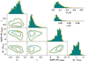 |
Fig. A.1. Corner plot: Correlation between SN Ia light-curve stretch (x1), colour (c), host mass and environmental local colour for the data (teal) and our realistic simulations (orange). Lines in the non-histogram panels show the contours containing 90% and 50% of the data (teal) and simulated points (orange). Top-right: Distribution of the stretch and colour errors following the corner-plot colour code. |
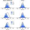 |
Fig. A.2. Left: Difference between the fitted (α, β, γ) and the input value when using a usual log-likelihood minimisation code, in σ. The stacked histograms corresponds to three different input values defined in the legend on the right. The black line is the model the histogram should follow if the results were unbiased (both values and error), which is a Gaussian with a null mean and unitary standard deviation. Right: Same as the left plot, but for the total-χ2 method. |
A.2. Significance of the broken magnitude-stretch relation
We use our simulation tool to further test the veracity of the broken-α model. We simulated data using a single α, fitted for a broken relation that split at the expected x1 = −0.5, and then computed the odds to find such a strong difference in α between the low and high-stretch modes.
We thus simulated 1,000 samples of 927 SNe using a linear α, setting α = 0.17, i.e. close to the one found in the ZTF sample while fitting a single α, and then performed the broken-α fit. We show in Fig. A.3 the resulting distribution of the fitted αlow and αhigh. They are accurately recovered in close agreement with the input αlow = αhigh = 0.17. The αlow = 0.271 ± 0.011 and αhigh = 0.083 ± 0.009 fitted on our data (teal point in Fig. A.3) are thus confirmed to be significantly different, confirming the non-linearity of the residuals-stretch relation.
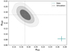 |
Fig. A.3. αlow vs αhigh when fitting a broken-α on samples simulated with a linear α. The dashed lines represent the input values. The contours (respectively 50%, 84% and 97%) are computed with 1000 simulations of a sample of a similar size to the one used throughout the paper, and the data point represents the values from the fit in Sect. 4.5. |
A.3. Difference between the step fitting methods
We investigated the step values obtained with the different methods described in Sect. 5, to validate that the discrepancies seen between the steps were due to variations in the fitting procedures. We used the simulations presented in Appendix A, with a broken-α and a local colour step of γ = 0.16 mag. The results are presented in Fig. A.4. The order of the points seen in the data is well reproduced by the simulations. Indeed, the ’Fixed (α, β)’ step is the smallest of the four steps, while the other three steps are all compatible. The factor between the regular step (’joint fit for (α, β, γ)’) and the ’fixed (α, β)’ step is the same in the data and in the simulations. The data exhibits a step difference of Δγ = 0.055 ± 0.027 mag, while the simulations exhibits a Δγ = 0.052 ± 0.024 mag difference (a 0.05σ difference between data and simulations). In the simulations, the broken-α step is of the same order as the regular linear-α step, while it is slightly higher in the data, with a reduced errorbar. However, we know the link between step and environment is more complex than the current model used in simulations and, since environment strongly correlates with stretch, this will likely impact the broken-α step. The further modelling of an age step will be the subject of a future analysis.
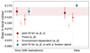 |
Fig. A.4. Local colour step for the four fitting procedures presented in Fig. 10, with 500 realisations of the simulations described in Appendix A.3 (left) and data (right). The points for the simulations are the means of the realisations, and the errorbars are the standard deviation. |
All Tables
Stretch correction coefficient (α) and absolute magnitude (M0) as a function of the SN environment.
Amplitude of the environment magnitude offset, aka steps, for the joint fit for (α, β, γ), without and with broken-α.
All Figures
|
Fig. 1. Top: Ideogram of the stretch distribution for the full sample (in grey), and for SNe in locally red and blue environments (509 and 429 SNe). The full grey line is the bimodal Gaussian from N21 described in Sect. 3, while the red and blue lines are bimodal Gaussian fits to the old and young progenitor subpopulations. Bottom: Stretch vs redshift, z. The fact that there is no depletion of low stretch SNe at a higher redshift is a consequence of the volume-limited cut. |
| In the text | |
|
Fig. 2. Correlation between SN Ia light-curve stretch (x1) and host stellar mass (top), as well as the local environment colour (bottom). The contours show the area containing 97%, 84%, and 50% of the SNe Ia. Vertical lines show the environment splitting values, while the horizontal lines show x1 = −0.5, the typical transition point between stretch modes (see Fig. 1). |
| In the text | |
|
Fig. 3. Connections between SN Ia light-curve stretch (x1), global stellar mass (log(M*/M⊙)global), and local environmental colour ((g − z)local), illustrating the complex correlation between stretch and SN environmental properties. Left: Local colour vs global host stellar mass. The light grey band shows the 25%–75% percentile range for host global mass (vertical, [9.5, 10.5] dex) and local environmental colour (horizontal, [0.7, 1.3] mag). These cuts are used to select SNe Ia shown in the right panels. Top-right: Local environmental colour and SN stretch distributions for SNe Ia whose host global mass is in [9.5, 10.5] dex. Blue and red histograms show locally blue and red environment SNe Ia. The black histogram is the local colour distribution for the full sample. Bottom-right: Global host stellar mass and SN stretch distributions for SNe Ia whose local environmental colour is in [0.7, 1.3] mag. Purple and green histograms show low and high mass hosts SNe Ia. |
| In the text | |
|
Fig. 4. SN Ia light-curve stretch (x1), global host mass (log(M*/M⊙)global), and local environmental colour ((g − z)local) distributions split per redshift origin. SNe Ia with galaxy redshifts are plotted in green (σz ∼ 10−4), and SNe Ia relying on low-resolution SN spectra (extracted from SEDm, Blagorodnova et al. 2018), either from SNID (Blondin & Tonry 2007) or on host emission lines are plotted in red (σz ∼ 10−3). The apparent stretch offset is explained by the selection function associated with galaxy redshifts, which favours high-mass hosts. |
| In the text | |
|
Fig. 5. Fraction of SNe in the high stretch mode as a function of the local colour, as modelled in Eq. (2). |
| In the text | |
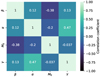 |
Fig. 6. Correlation matrix of the standardisation parameters from Eq. (5). |
| In the text | |
|
Fig. 7. Histogram of the standardised Hubble residuals (corrected for SN colour, SN stretch, and environment). The blue line is a Gaussian centred on 0 with a standard deviation corresponding to the normalised median absolute deviation σnmad = 0.176. |
| In the text | |
|
Fig. 8. Standardised Hubble residuals (α = 0) as a function of stretch (x1). Large blue points show the data binned by stretch (mean) while the red hexagons show the binned stretch for SNe Ia from locally red environments. The errorbars on the binned points only display the error on the mean, but a reference for the fitted intrinsic scatter σint is plotted in the top-right corner. The blue line shows the best fitted broken-α model, while the dashed grey line shows the best α when assuming the linear Tripp relation. |
| In the text | |
|
Fig. 9. Standardised Hubble residuals corrected for stretch (with a broken-α) and colour as a function of local environmental colour. Large blue points show the residuals binned by local colour, with the errorbars corresponding to the error on the mean. The scale of the fitted intrinsic scatter is shown in the top-right corner. The dashed line shows the step model. The full line illustrates the step model once convolved by a Gaussian with a standard dispersion equals to the mean local environmental measurement error (σ(g − z),local ∼ 0.14), as we account for those errors in the step model. |
| In the text | |
|
Fig. 10. Fitted steps for each of the environmental proxies. The dark red and green points indicate steps where both (α, β) and γ are fitted at the same time for each proxy. The light red points indicate the steps when the same (α, β) correction (fixed across proxies) is applied to the whole sample. The red points indicate the steps when independent (α, β) corrections are applied for each of the subsamples. The green points are steps when including the broken-α model into the fit, according to Sect. 4.5. The shaded band represents the 1σ interval for the reference step (local colour step from the joint fit). |
| In the text | |
|
Fig. 11. Hubble residuals corrected for colour and environment as a function of stretch x1 (same as Fig. 8), for the full sample (white points) and blue and red SNe (blue and red points). |
| In the text | |
|
Fig. A.1. Corner plot: Correlation between SN Ia light-curve stretch (x1), colour (c), host mass and environmental local colour for the data (teal) and our realistic simulations (orange). Lines in the non-histogram panels show the contours containing 90% and 50% of the data (teal) and simulated points (orange). Top-right: Distribution of the stretch and colour errors following the corner-plot colour code. |
| In the text | |
|
Fig. A.2. Left: Difference between the fitted (α, β, γ) and the input value when using a usual log-likelihood minimisation code, in σ. The stacked histograms corresponds to three different input values defined in the legend on the right. The black line is the model the histogram should follow if the results were unbiased (both values and error), which is a Gaussian with a null mean and unitary standard deviation. Right: Same as the left plot, but for the total-χ2 method. |
| In the text | |
|
Fig. A.3. αlow vs αhigh when fitting a broken-α on samples simulated with a linear α. The dashed lines represent the input values. The contours (respectively 50%, 84% and 97%) are computed with 1000 simulations of a sample of a similar size to the one used throughout the paper, and the data point represents the values from the fit in Sect. 4.5. |
| In the text | |
|
Fig. A.4. Local colour step for the four fitting procedures presented in Fig. 10, with 500 realisations of the simulations described in Appendix A.3 (left) and data (right). The points for the simulations are the means of the realisations, and the errorbars are the standard deviation. |
| In the text | |
Current usage metrics show cumulative count of Article Views (full-text article views including HTML views, PDF and ePub downloads, according to the available data) and Abstracts Views on Vision4Press platform.
Data correspond to usage on the plateform after 2015. The current usage metrics is available 48-96 hours after online publication and is updated daily on week days.
Initial download of the metrics may take a while.