© The Authors 2023

1. Introduction

The standard model of cosmology assumes that gravity is described at all scales by general relativity (GR) and its content is dominated by two exotic components, cold dark matter (CDM) and a dark energy component with the dynamics of a cosmological constant Λ. These components are required to explain the growth of structures and the acceleration of the expansion of the Universe. This flat ΛCDM+GR model has been successful in describing most, if not all, cosmological observations.

The exact nature of dark energy remains unknown, and alternative models of gravity have been proposed to explain our observations without needing dark energy (see e.g., Clifton et al. 2012; Zhai et al. 2017; Ezquiaga & Zumalacárregui 2018). These models can predict the same background quantities as the ΛCDM+GR model, such as the expansion rate H(z) as a function of redshift z, but they can yield quite different predictions for quantities related to perturbations, such as the linear growth rate of structures f(z). In some of these models, the growth rate even becomes scale dependent. To test whether our Universe is ruled by a ΛCDM+GR model or some alternate gravity model, not only do we need precise measurements of H(z) from standard candles (e.g., type-Ia supernovae) or standard rulers (e.g., baryon acoustic oscillations) but also measurements of the growth of structures f(z) with redshift-space distortions or of the amplitude of matter fluctuations with weak gravitational lensing. Ongoing and future cosmological surveys will constrain the expansion rate to subpercent level precision and the growth rate to a few percent which will allow us to test models of gravity.

Most common measurements of the growth rate of structures are based on the effect of redshift-space distortions in the clustering of galaxies (Guzzo et al. 2008; Song & Percival 2009). Peculiar velocities of galaxies modify their cosmological redshift, such that when we estimate distances to these galaxies using their observed redshifts, they are slightly misplaced relative to their true comoving positions. The galaxy density field becomes distorted in redshift space relative to real comoving space, and the two-point statistics of the galaxy density field becomes anisotropic: the clustering along the line of sight is enhanced relative to the clustering across the line of sight. The amplitude of this anisotropy is proportional to the growth rate f and to the amplitude of matter fluctuations, commonly described by the σ₈ parameter (the standard deviation of the matter field that has been top-hat smoothed on scales of 8 h⁻¹Mpc). Clustering measurements of growth therefore usually quote the combination f(z)σ₈(z). Several redshift-space distortion measurements have been performed in the past decade by spectroscopic surveys including WiggleZ (Blake et al. 2011), 6dFGRS (Beutler et al. 2012), SDSS-II (Samushia et al. 2012), SDSS-MGS (Howlett et al. 2015), FastSound (Okumura et al. 2016), VIPERS (Pezzotta et al. 2017; de la Torre et al. 2017), SDSS-III BOSS (Beutler et al. 2017; Grieb et al. 2017; Sánchez et al. 2017; Satpathy et al. 2017), and more recently by SDSS-IV eBOSS (Bautista et al. 2021; Gil-Marín et al. 2020; de Mattia et al. 2021; Tamone et al. 2020; Hou et al. 2021; Neveux et al. 2020). The latest measurements of fσ₈ with redshift-space distortions reach uncertainties of about 10 percent and currently no deviations from ΛCDM+GR have been detected (Alam et al. 2021).

Another method to measure fσ₈ is to derive it from the two-point statistics of direct peculiar velocity estimates for individual galaxies (Gorski et al. 1989; Strauss & Willick 1995). Peculiar velocities can be measured if both redshifts and absolute distances can be estimated independently. While spectroscopy provides precise redshifts, distance estimates can be obtained using well-known correlations such as the Tully-Fisher relation for spiral galaxies (TF, Tully & Fisher 1977) or the Fundamental Plane for elliptical ones (FP, Djorgovski & Davis 1987). Such distances can be measured for galaxies at relatively low redshifts (z < 0.1) since uncertainties quickly increase with redshift. Current state-of-the-art samples of TF and FP distances include CosmicFlows4 (Tully et al. 2023) and the SDSS-FP sample (Howlett et al. 2022), both containing a few times 10⁴ distance measurements. The statistical properties of a sample of peculiar velocities can be measured alone or in combination with an overlapping galaxy density field, analogously to a multitracer analysis. Several methods have been developed in the past years to extract growth-rate measurements from sets of peculiar velocities: The maximum-likelihood method, where velocity (and density) fields are assumed to be drawn from multivariate Gaussian distributions (Johnson et al. 2014; Huterer et al. 2017; Howlett et al. 2017a; Adams & Blake 2020; Lai et al. 2023). This is the method we employ in this work; The compressed two-point statistics such as two-point correlation function, power spectrum, or average pair-wise velocities (Nusser 2017; Dupuy et al. 2019; Qin et al. 2019; Turner et al. 2022); The comparison between observed velocities to those reconstructed from a density field (Davis et al. 2011a; Carrick et al. 2015; Boruah et al. 2020; Said et al. 2020); The field level inference by evolving initial conditions or forward modeling method (Boruah et al. 2022; Prideaux-Ghee et al. 2023).

Type-Ia supernovae (SNe Ia) are well-known standardizable candles that have smaller intrinsic scatter in standardized peak luminosity (of about 15 percent) than TF and FP relations (of about 40 percent), so SNe Ia can yield more precise peculiar velocities. SNe Ia have only been marginally used for growth-rate measurements (e.g., Boruah et al. 2020) since most surveys only cover small parts of the sky or suffer from being compilations of several different telescopes, which cover the sky inhomogeneously (e.g., Betoule et al. 2014; Scolnic et al. 2022). Photometric surveys with high cadence and large sky coverage, such as the Zwicky Transient Facility (ZTF, Graham et al. 2019) and the Rubin Observatory Legacy Survey of Space and Time (Rubin-LSST, LSST Science Collaboration 2009) will provide a large and uniform sample of SNe Ia that can be used for peculiar velocity studies (Howlett et al. 2017a). Combining peculiar velocities from SNe Ia, Tully-Fisher and Fundamental Plane can set the best constraints on the growth-rate at z < 0.1 and will allow us to constrain alternatives to GR (Kim & Linder 2020; Lyall et al. 2022).

In this work we study the possibility for a first growth-rate measurement using uniquely SN Ia data from ZTF. In preparation for the analysis of these data, we produced realistic simulations of ZTF SN Ia light-curves, including selection effects and instrumental noise, and we performed the analysis required to derive fσ₈, based on the maximum likelihood method (Johnson et al. 2014; Howlett et al. 2017a).

This article is organized as follows. In Sect. 2 we describe the pipeline to produce ZTF simulations of SN Ia observations. In Sect. 3 we present the method used to estimate fσ₈. In Sect. 4 we describe our main findings. In Sect. 5 we consider variations of the baseline analysis. We finally conclude in Sect. 6.

2. ZTF simulations

This section describes our framework to produce realistic sets of simulated SN Ia light-curves from the Zwicky Transient Facility, including peculiar velocities and multiple possible observational effects. Our pipeline goes through the following steps: 1) we extract host catalogs from a suitable N-body simulation; 2) we generate SN Ia events with positions drawn from the host catalog and random dates; 3) we generate their true light-curve parameters; 4) we simulate ZTF-like light-curves based on real observations (cadence, filters, noise); 5) we introduce ZTF-like spectroscopic selection effects; 6) we apply ZTF-like quality cuts on selected observations. Each of these steps are described in detail below. This pipeline, named SNSIM¹, was implemented in python language and is publicly available. Another alternative software for producing ZTF simulations is SIMSURVEY² (Feindt et al. 2019). SIMSURVEY was previously used to study the discovery rates of different transients before the start of the survey.

2.1. The N-body simulation

To study the statistics of realistic nonlinear velocity fields, we rely on velocities from halos found in matter-only N-body simulations that are publicly available.

We used the OuterRim³ cosmological simulation (Heitmann et al. 2019) and focused on the snapshot at redshift z = 0. The OuterRim simulation was widely used in recent cosmological measurements from the eBOSS (Gil-Marín et al. 2018; Hou et al. 2018; Zarrouk et al. 2018; Avila et al. 2020; Rossi et al. 2021; Smith et al. 2020). The OuterRim volume is a (3 h⁻¹Gpc)³ cubic box. A total of 10,240³ particles were evolved from initial conditions set at z = 200 using the Zeldovich approximation and cosmological parameters displayed in Table 1. This corresponds to a particle mass m_p = 1.85 × 10⁹h⁻¹ M_⊙.

Halos were defined using a friend-of-friends algorithm with a linking length of b = 0.168, resulting in 1.9 × 10⁹ halos with masses. typically ranging from m_10% ∼ 4 × 10¹⁰ M_⊙ (10th percentile) to m_90% ∼ 4.6 × 10¹¹ M_⊙ (90th percentile).

In the rest of this work, we assign SNe Ia to halo positions with a probability that is independent of halo mass.

We have produced 27 realizations by selecting (1 h⁻¹ Gpc)³ subboxes. Each subbox encloses halos up to z ∼ 0.17 when we place the observer at its center. We show in Sect. 2.5 that after all the selection effects we do not observe spectroscopically typed SN Ia above z ∼ 0.14 in the ZTF survey.

We did not attempt to populate halos with a realistic sample of galaxies, even though potential effects can be introduced due to correlations of supernova events with type of galaxy (passive or star-forming) and how these galaxies connect to large-scale structures. We leave this investigation for future work.

2.2. From N-body mocks to a survey-like host catalog

From the N-body simulation mocks, we convert spatial comoving coordinates of halos (x, y, z) to right-ascension (RA), declination (Dec) and redshift (z_cos). We first placed the observer at the center of each (1 h⁻¹Gpc)³ subbox and computed distances of each halo to the observer.

To convert distances to cosmological redshifts z_cos we numerically invert the redshift-comoving distance relation, which for a flat ΛCDM universe is given by

$$\begin{array}{c}\hfill r_{\text{cos}}\equiv r(z_{\cos })=\frac{c}{H_0}{\displaystyle {\int }_0^{z_{\cos }}}\frac{\mathrm{d}z}{\sqrt{{\mathrm{\Omega }}_m{(1+z)}^3+{\mathrm{\Omega }}_{\mathrm{\Lambda }}}},\end{array}$$(1)

where Ω_m and Ω_Λ are respectively the density of matter and dark energy today. Since we assume a flat universe Ω_Λ = 1 − Ω_m.

We then take into account the Doppler effect due to the peculiar velocity of the host and the velocity with respect to the Cosmic Microwave Background (CMB) frame to obtain the observed redshift z_obs as

$$\begin{array}{c}\hfill (1+z_{\mathrm{obs}})=(1+z_{\cos })(1+z_{\mathrm{p}})(1+z_{\odot }),\end{array}$$(2)

where z_cos is the cosmological redshift, z_p the red(or blue)shift due to the host peculiar velocity and z_⊙ is the shift due to the peculiar velocity of the Solar System with respect to CMB restframe. We set z_⊙ = 0 considering that it can be corrected using CMB measurement (Planck Collaboration I 2020).

The expression for z_p derives from the relativistic Doppler effect due to the peculiar velocity and is given by

$$\begin{array}{c}\hfill 1+z_{\mathrm{p}}=\frac{1+{\mathbf{v}}_p·\widehat{}\}n/c}{\sqrt{1-{(||{\mathbf{v}}_p||/c)}^2}},\end{array}$$(3)

where v_p is the 3-D peculiar velocity vector, c the speed of light, and $\widehat{\mathbf{n}}$ is the unit vector pointing toward the SN Ia. The second-order term (||v_p||/c)² can be neglected, leading to

$$\begin{array}{c}\hfill z_{\mathrm{p}}=\frac{{\mathbf{v}}_{\mathbf{p}}·\widehat{\mathbf{n}}}{c}.\end{array}$$(4)

This last expression allows us to compute the line-of-sight velocity from the Doppler shift.

The relativistic beaming due to peculiar velocities change the luminosity distance d_L (Hui & Greene 2006; Davis et al. 2011b) as

$$\begin{array}{c}\hfill d_{L,\text{obs}}={(1+z_{\mathrm{p}})}^2{d}_{L,\text{cos}},\end{array}$$(5)

where d_L, cos ≡ d_L(z_cos) = (1 + z_cos)r_cos is the cosmological luminosity distance. The observed distance modulus is then given by

$$\begin{array}{cc}\hfill {\mu }_{\mathrm{obs}}& =5log\left(\frac{d_{L,\text{obs}}}{10\mathrm{pc}}\right)\hfill \end{array}$$(6)

$$\begin{array}{cc}& =5log\left({(1+z_{\mathrm{p}})}^2\frac{d_{L,\cos }}{10\mathrm{pc}}\right)\hfill \end{array}$$(7)

$$\begin{array}{cc}& ={\mu }_{\cos }+10log(1+z_{\mathrm{p}}).\hfill \end{array}$$(8)

Figure 1 illustrates these two effects on a random sample of distance indicators with Gaussian realizations of their peculiar velocities. The effect on the observed redshifts is proportional to (1 + z_p) while the effect on distance moduli is logarithmic, so subdominant (as seen in the snippet of Fig. 1).

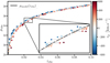Fig. 1. Toy model illustrating how peculiar velocities impact the observed redshift zobs and the observed distance moduli μobs. Radial peculiar velocities are randomly drawn from a Gaussian distribution with σvp = 300 km s−1. The color of each point indicates the value of its radial peculiar velocities vp. The effect on the x-axis is of first order on vp while the effect on the y-axis is of second order.

2.3. Generating SN Ia events

The next step is to generate type-Ia supernova events. We used the latest estimates for the rate of explosions,

$$\begin{array}{c}\hfill r_{v,P20}(z=0)=(2.35\pm 0.24)\times {10}^{-5}{\text{Mpc}}^{-3}{\text{yr}}^{-1},\end{array}$$(9)

measured from ZTF data (Perley et al. 2020). We rescaled this rate to our fiducial H₀ value with r_v = r_v, P20(h/0.70)³. We also account for the time dilation at z > 0 by scaling the rate by 1/(1 + z). From this rate we computed the average number of SNe Ia given the volume and the duration of our survey. We then drew the number of SNe Ia in a given realization using a Poisson law.

These SN Ia events were spatially assigned to the halos positions from the N-body simulation. The velocity of the halos were also directly assigned to their corresponding SN Ia. This procedure neglects the velocity contribution from the relative velocity between the SN Ia and its host, which would simply add extra intrinsic scatter to their velocities.

To generate the light-curves, we used the SALT2.4 model (Guy et al. 2007, 2010), which parameterized them by their stretch x₁, color c and peak-magnitude in the Bessel-B band m_B. Using the Tripp relation (Tripp 1998), the rest-frame magnitude in Bessel-B band for a given SN (indexed by the subscript i) is

$$\begin{array}{c}\hfill M_{B,i}^{\ast }=M_B-\alpha x_{1,i}+\beta c_i+{\sigma }_{\mathrm{int},i},\end{array}$$(10)

where α, β and M_B are common to all SNe Ia and x_1, i, c_i and the intrinsic scattering σ_int, i are randomly drawn from distributions described below.

The absolute magnitude of SNe Ia in Bessel-B band M_B, defined in the AB magnitude system, is fixed at the best-fit value of −19.05 (for H₀ = 70 km s⁻¹ Mpc⁻¹ from Betoule et al. 2014). We rescaled this M_B value to our fiducial cosmology using

$$\begin{array}{c}\hfill M_B=-19.05+5log\left(\frac{h}{0.7}\right).\end{array}$$(11)

The α and β parameters are also fixed to best-fit values from Betoule et al. (2014) that are α = 0.14 and β = 3.1. The stretch parameter x₁ distribution is modeled using the redshift dependent two-Gaussian mixture from Nicolas et al. (2021). The color parameter c distribution follows the asymmetric model given by Table 1 of Scolnic & Kessler (2016) for low-z (G10 model). The intrinsic scattering σ_int is drawn from a normal distribution with dispersion fixed to σ_M = 0.12. The values for the main input parameters are summarized in Table 2.

After generating x₁, c and σ_int for each SN Ia, we compute their apparent magnitude given by

$$\begin{array}{c}\hfill m_B=M_B^{\ast }+{\mu }_{\mathrm{obs}},\end{array}$$(12)

where μ_obs is the observed distance modulus to the SN Ia host (Eq. (8)), which includes the peculiar velocity contribution.

2.4. Replicating ZTF observations

The Zwicky Transient Facility (ZTF) is conducting a photometric survey using the Samuel Oschin 48-inch (1.2-m) Schmidt Telescope at the Palomar observatory (Graham et al. 2019). It covers the entire northern visible sky in the g, r and i bands with 30-second exposures pointing a fixed grid of fields with minimal dithering (Bellm et al. 2019). The ZTF camera hosts 16 charge coupled devices (CCD) containing a total of 0.6 gigapixels with an effective field of view of ≃47 deg². We use the focal plane dimensions, including inter-CCD gaps from Dekany et al. (2020) (Table 3).

The data processing pipelines are managed by Infrared Processing and Analysis Center (IPAC, Masci et al. 2019), which provides metadata tables. In order to replicate ZTF observations we query these metadata using the public code ZTFQUERY⁴.

The essential quantities of our simulations are: the dates of observations; the filters used; the limiting magnitude at 5-σ of the observations m_5σ, which defines the magnitude at which the signal-to-noise ratio (S/N) is equal to 5; the CCD gain G of each observation in units of electrons per analog-to-digital unit (ADU); the zero point ZP of each observation which gives the magnitude of an object that produces a flux of 1 ADU during an exposure. We also account for the Milky-Way dust extinction using the CCM89 model (Cardelli et al. 1989) and computing each object EBV from the Schlegel et al. (1998) dust map implemented in the pyhton package SFDMAP⁵.

We obtained true fluxes for each epoch of ZTF observations using SNCOSMO package⁶ (Barbary et al. 2016). Since the flux noise is dominated by the sky background at high-magnitude, we compute an effective sky noise using the limiting magnitude:

$$\begin{array}{c}\hfill {\sigma }_{\mathrm{sky}}=\frac{1}{5}{10}^{-0.4(m_{5\sigma }-\text{ZP})}.\end{array}$$(13)

A random noise is added to the true flux of each epoch. This noise is drawn from a Gaussian distribution with standard deviation given by

$$\begin{array}{c}\hfill {\sigma }_F^2=\frac{F}{G}+{\sigma }_{\mathrm{sky}}^2+{\left(\frac{ln(10)}{2.5}F\right)}^2{\sigma }_{\text{ZP}}^2,\end{array}$$(14)

where we set σ_ZP = 0.01 as a calibration uncertainty. This calibration uncertainty will be refined in further works, together with taking into account host background, brighter-fatter effect, point spread function effects and calibration uniformity.

Figure 2 displays examples of simulated light-curves from ZTF SN Ia events, at three redshifts. We note that since i-band observations are not performed over the whole sky, some supernovae have few or no i-band observations as the one shown in the bottom panel of Fig. 2.

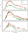Fig. 2. Examples of simulated ZTF light-curves of type-Ia supernovae at low, intermediate and high redshifts. Points with error bars are the simulated data, and the solid lines are the input light-curves.

We simulated a 6-year data sample, similar to the full ZTF survey duration. We used observation metadata from 2018-06-19 to 2022-08-31, to follow realistic observing conditions. To obtain a 6-year simulated survey, we artificially increased the SN Ia rate.

2.5. ZTF selection from detection and spectroscopic typing

For cosmological analysis we require that detected objects are confirmed as type-Ia supernovae. The ZTF Bright Transient Survey (BTS) is a spectroscopic campaign to spectroscopically classify extragalactic transients brighter than 18.5 mag at peak brightness in either the g or r-filters (Fremling et al. 2020; Perley et al. 2020). The BTS follow-up procedure requires stringent cuts, we describe their implementation in this section.

Prior to spectroscopic selection we performed a photometric detection of sources by discarding SN Ia light-curves with less than two epochs with fluxes S/N above 5. In order to simulate the BTS spectroscopic selection effect, we followed bullets 1 to 3 of the procedure presented in Sect. 2.3 of Perley et al. (2020): 1) prior to peak brightness, at least one observation with −16.5 < t − t_peak < −7.5 days; 2) around peak brightness, at least one observation with −7.5 < t − t_peak < −2.5 or 2.5 < t − t_peak < 7.5; 3) after peak brightness, at least one observation with 7.5 < t − t_peak < 16.5 or two observations, one within 2.5 < t − t_peak < 7.5 and one within 16.5 < t − t_peak < 28.5. Where t_peak is defined as the time where the light-curve reaches maximum flux (provided it has S/N above 5).

At higher magnitude the spectroscopic efficiency drops. To simulate this, we used the completeness given in Fig. 4 of Perley et al. (2020) to randomly discard objects as a function of their peak magnitude.

Figure 3 shows the SN Ia angular distribution of a single mock realization of the ZTF 6-year survey, before and after selection effects. The parent sample (blue dots) uniformly covers the northern sky at Dec > −30 deg, by construction. Photometry and spectroscopy preferentially select SN Ia events outside the Galactic plane.

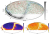Fig. 3. Angular distribution and completeness of the simulated ZTF SN Ia sample. Top: angular distribution of simulated ZTF type-Ia supernova from one mock realization of a 6-year program. The parent sample of simulated SNe Ia is shown in blue, those detected in photometry are shown in green and those successfully typed with spectroscopy are shown in red. A map of stellar density from the Gaia satellite is shown in the background. Bottom: angular completeness of photometric (left) and spectroscopic samples (right). The photometric completeness is computed relative to the parent sample while the spectroscopic one is relative to those detected in photometry, using the full redshift range of the simulation, that is 0 < z < 0.14. Different ranges are used for the color scales.

We estimated the sky coverage of each sample and defined their completeness. The sky coverage is calculated by assigning SNe Ia of 27 mock realizations to an angular mesh provided by the HEALPIX⁷ software (Górski et al. 2005; Zonca et al. 2019), which yields pixels of equal area. Using 12,288 pixels (n_side = 32), we estimated that the parent sample covers uniformly an area of 31537.3 deg². The photometric and spectroscopic samples cover respectively 30698.0 and 28700.5 deg². Since photometric and spectroscopic samples are subsamples of the parent sample, we can estimate their completeness by computing the ratio of the number of SNe Ia in each sample to the same number in the parent sample, in each angular pixel. Bottom panels of Fig. 3 display two ratios: photometric to parent and spectroscopic to photometric. While photometric completeness is nearly 40% of the extra-Galactic sky, the spectroscopic completeness is around 6 percent, mainly due to the magnitude cut imposed for follow-up. Naturally these completeness values are dependent on the maximum redshift of the simulation, that is z = 0.17.

Figure 4 displays the redshift distribution of simulated SNe Ia before and after selections caused by photometric detection and spectroscopic follow-up. The top panel shows the absolute number of SNe Ia per redshift bin while the bottom panel shows the comoving number density n(z) of SNe Ia as a function of redshift, for which we see even more clearly the impact of the photometric detection and spectroscopic selection. This density is the quantity of interest for clustering measurements. We computed these densities as the ratio of the number of SNe Ia in a redshift bin to its corresponding comoving volume. The volume calculation assumes the fiducial cosmology from Table 1, in order to convert redshifts into distances, and the angular masks estimated above, shown in Fig. 3. In Fig. 4 we see that the rate of explosions for the parent sample has a slight dependency on redshift due to the time dilation factor 1/(1 + z). While the photometric sample extends to redshifts beyond z = 0.15, the density of the spectroscopic sample quickly drops beyond z = 0.06.

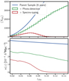Fig. 4. Number and density distributions of SNe Ia with respect to redshift. The parent sample of simulated SNe Ia is shown in blue, those detected in photometry are shown in green and those successfully typed with spectroscopy are shown in red. Top panel: number of simulated ZTF type-Ia supernova versus redshift per bins of Δzobs = 0.005, averaged over 27 independent mock realizations of a 6-year program. Bottom panel: comoving number density of SNe Ia versus redshift, calculated assuming the fiducial cosmology from Table 1.

2.6. Light-curve parameter adjustment and quality cuts

Each simulated SN Ia light-curve is fit using the same framework (SALT2) that was used to generate them with the SNCOSMO package implementation. For each light-curve, we fit for the stretch x₁, color c, peak-magnitude m_B, and time of peak-brightness t₀. The redshift z_obs of host galaxies is assumed to be provided by an external spectroscopic survey. We fixed it to its true value during the fit as we assume the error to be negligible. The covariance matrix C_SALT, i of the fit is defined by

$$\begin{array}{c}\hfill C_{\mathrm{SALT},i}=\left(\begin{array}{ccc}{\sigma }_{m_B,i}^2& {\mathrm{Cov}}_{m_B{x}_1,i}& {\mathrm{Cov}}_{m_{B}c,i}\\ {\mathrm{Cov}}_{m_B{x}_1,i}& {\sigma }_{x_1,i}^2& {\mathrm{Cov}}_{x_{1}c,i}\\ {\mathrm{Cov}}_{m_{B}c,i}& {\mathrm{Cov}}_{x_{1}c,i}& {\sigma }_{c,i}^2\end{array}\right),\end{array}$$(15)

and will be used when fitting for standardization parameters in Sect. 3.1.1.

Some of our fits did not converge during the first attempt for at least two reasons. Firstly, some fits with excessive χ² values correspond to light-curves with high S/N. To avoid this problem, we fit these light-curves by artificially increasing the flux uncertainties to help the minimizer to find the true minima. We then used these best-fit parameters as a first guess for a second iteration with the initial flux uncertainties. Secondly, some over-sampled light-curves show convergence problems, particularly when the oversampling occurs at the edges of the available phase range for the SALT2 model. When varying the peak-brightness time t₀ during the fit, it will also change the number of points considered in the fit. Refitting those light-curves by discarding points 5 days around the SALT2 model boundaries solved this issue.

The final step in creating a full ZTF simulation of SN Ia light-curves is to apply quality cuts that are commonly done for precision cosmological measurements. We followed the procedure adopted on real data, as described in the first data release of the ZTF Type Ia Supernova survey (Dhawan et al. 2022). Table 3 summarizes the selections made on light-curves as well as the fraction of objects passing each criterion. These fractions are obtained by averaging results from 27 independent mock realizations of the survey. The fraction of SNe Ia with converged SALT2 fits is given in the first row of Table 3. We selected only best-fit models describing the data with probability larger than 95 percent. In order to ensure a robust estimate of maximum brightness, we selected light-curves containing at least three exposures within 10 days of maximum brightness. We excluded any light-curve with best-fit stretch |x₁|< 3 or color |c|< 0.3. We also excluded light-curves for which the uncertainty in t₀ or x₁ is larger than 1. A final redshift cut z_obs > 0.02 is meant to avoid supernovae velocities to be correlated within our local flow.

After all cuts, the average number of SN Ia is ⟨N⟩∼3520 for our 6-year sample. This number correspond to the spectroscopically classified sample of SNe Ia.

3. Methodology

In this section we introduce the methodology employed in this work to measure the growth-rate of structures fσ₈ from peculiar velocities derived from a sample of standardized SNe Ia. We used the maximum-likelihood method which assumes that the peculiar velocity field is a Gaussian random field.

The Gaussian likelihood is expressed as

$$\begin{array}{cc}& \mathcal{L}(\mathbf{p},{\mathbf{p}}_{\mathrm{HD}})={(2\pi )}^{-\frac{n}{2}}{|C(\mathbf{p},{\mathbf{p}}_{\mathrm{HD}})|}^{-\frac{1}{2}}\hfill \\ \hfill & \times exp[-\frac{1}{2}{\mathbf{v}}^T({\mathbf{p}}_{\mathrm{HD}})C{(\mathbf{p},{\mathbf{p}}_{\mathrm{HD}})}^{-1}\mathbf{v}({\mathbf{p}}_{\mathrm{HD}})],\hfill \end{array}$$(16)

where v is the data vector containing the sampled peculiar velocity field, C(p, p_HD) is the covariance matrix describing correlations between velocities, p and p_HD are vectors containing the parameters of the model. p_HD refers to parameters of the Hubble diagram and SN Ia standardization and p refers to growth-rate related parameters including fσ₈. We subsequently describe these parameters in detail in the following sections.

Our methodology is based on works by Johnson et al. (2014), Howlett et al. (2017a), Adams & Blake (2020), Lai et al. (2023), who apply this methodology to samples of peculiar velocities derived from Tully-Fisher and Fundamental Plane distances. In this work we only applied this method to the velocity field, leaving the cross-correlation with a galaxy density field for future work.

We start this section by describing the construction of the data vector v containing peculiar velocities (Sect. 3.1), then the construction of the covariance matrix (Sect. 3.2).

3.1. The velocity data vector

Peculiar velocities of SN Ia hosts can be extracted via the residuals with respect to the Hubble diagram, as illustrated in Figs. 1 and 5. Here we present how we fit for the Hubble diagram parameters p_HD.

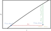Fig. 5. Representation of the different effects of peculiar velocities on the Hubble diagram for a single SN. The red dotted line shows the Doppler shift, the yellow line shows the relativistic beaming effect and the green dotted line shows the Hubble residual.

3.1.1. Hubble diagram and SN Ia standardization

Usually the fit of the Hubble diagram varies background cosmological parameters (e.g., Ω_m) as well as standardization parameters (α, β and M₀). However, given the small span of redshift of ZTF, we cannot constrain Ω_m. We can either fix the Hubble diagram by assuming true input cosmological parameters of the simulation or assume low-redshift linear relation. In this work we decided to fix the cosmology to simulation input, thus our Hubble diagram parameters are p_HD = {α, β, M₀, σ_M} and we only fit for the SN Ia standardization expressed by the Tripp relation:

$$\begin{array}{c}\hfill {\mu }_{\mathrm{obs},i}({\mathbf{p}}_{\mathrm{HD}})=m_{B,i}-(M_B-\alpha x_{1,i}+\beta c_i).\end{array}$$(17)

As shown on Figs. 1 and 5, the quantity of interest in order to derive peculiar velocities from SNe Ia is the Hubble diagram residuals which is the difference between the observed distance modulus and the model distance modulus evaluated at the observed redshift z_obs. Hubble residuals are given by

$$\begin{array}{c}\hfill \mathrm{\Delta }{\mu }_i({\mathbf{p}}_{\mathrm{HD}})={\mu }_{\mathrm{obs},i}({\mathbf{p}}_{\mathrm{HD}})-{\mu }_{\text{model}}(z_{\mathrm{obs},i}),\end{array}$$(18)

and their uncertainties by

$$\begin{array}{c}\hfill {\sigma }_{\mu ,i}^2({\mathbf{p}}_{\mathrm{HD}})={\mathbf{A}}_i{({\mathbf{p}}_{\mathrm{HD}})}^T{C}_{\mathrm{SALT},i}{\mathbf{A}}_i({\mathbf{p}}_{\mathrm{HD}})+{\sigma }_M^2,\end{array}$$(19)

where the vector A_i is given by

$$\begin{array}{c}\hfill {\mathbf{A}}_i({\mathbf{p}}_{\mathrm{HD}})=\left(\begin{array}{c}1\\ \alpha \\ -\beta \end{array}\right),\end{array}$$(20)

and the covariance C_SALT, i is written in Eq. (15).

3.1.2. Peculiar velocities from Hubble residuals

From Eq. (15) of Hui & Greene (2006) we can show that a first-order expansion of Hubble diagram residuals (18) with respect to peculiar velocities gives the estimator (see Appendix A.1):

$$\begin{array}{c}\hfill {\widehat{v}}_i({\mathbf{p}}_{\mathrm{HD}})=-\frac{ln(10)c}{5}{(\frac{(1+z_i)c}{H(z_i)r(z_i)}-1)}^{-1}\mathrm{\Delta }{\mu }_i({\mathbf{p}}_{\mathrm{HD}}).\end{array}$$(21)

Although the derivation of the estimator gives that z_i is evaluated as the cosmological redshift z_i = z_cos, i, as stated in Hui & Greene (2006) replacing it by z_obs is only a second order approximation. Since we do not have access to cosmological redshifts, we used the observed redshift z_i = z_obs, i to estimate velocities. However, the estimator is valid in a regime where the peculiar redshift z_p is small enough compared to the cosmological redshift z_cos. This leads to small biases on velocity estimates, in particular for nearby galaxies with high velocities. We further discuss this point in Appendix A.2. This estimator is used in Johnson et al. (2014) but throughout the literature other variants of this estimator including more approximations have been used. In Appendix A.2, we also compare performances of different estimators. We concluded that the bias is small for all of them but we choose to use (21) since it is the least biased. However this estimator depends on the cosmological model used, and using cosmological parameters that differ from the true ones will result in a bias of the velocity estimator. In Appendix A.3 we evaluate this bias as a function of Ω_m and we conclude that it is negligible.

We compute the uncertainty on our velocity estimations as

$$\begin{array}{c}\hfill {\sigma }_{\widehat{v},i}({\mathbf{p}}_{\mathrm{HD}})=\frac{ln(10)c}{5}{(\frac{(1+z_{\mathrm{obs},i})c}{H(z_{\mathrm{obs},i})r(z_{\mathrm{obs},i})}-1)}^{-1}{\sigma }_{\mu ,i}({\mathbf{p}}_{\mathrm{HD}}).\end{array}$$(22)

In the low-redshift limit, this error grow quasi-linearly with redshift:

$$\begin{array}{c}\hfill {\sigma }_{\widehat{v}}\simeq 1400\left(\frac{z}{0.1}\right)\left(\frac{{\sigma }_{\mu }}{0.1}\right)\mathrm{km}{\mathrm{s}}^{-1}.\end{array}$$(23)

All biases that we underline in the previous paragraph are below ∼5% for a typical velocity of v ∼ 300 km s⁻¹.

3.2. The covariance matrix

The modeling of the statistical properties of our sample of peculiar velocities is made through the covariance matrix C(p, p_HD) of the Gaussian likelihood from Eq. (16). This covariance can be decomposed in two parts: an analytical part, which depends on a theoretical modeling of the large-scale cosmological correlations of velocities, and an observational part which accounts for observational uncertainties.

3.2.1. Modeling large-scale cosmological correlations

The analytical part of the covariance C^vv will depend on the growth-rate parameter fσ₈, and other nuisance parameters, which will be varied altogether when maximizing the likelihood. Each element of the covariance matrix $C_{\mathit{ij}}^{\mathit{vv}}\equiv ⟨v_i{v}_j^{\ast }⟩$ is defined as the correlation function of the radial velocity field at two positions r_i and r_j. This correlation can be written as an inverse Fourier transform of the velocity-velocity correlations in Fourier space. The radial component v_i of the three-dimensional velocity field v(r) at a position r_i can be written as:

$$\begin{array}{c}\hfill v_i={\widehat{\mathbf{r}}}_i·\mathbf{v}({\mathbf{r}}_i)={\displaystyle \int }\frac{{\text{d}}^{3}k}{{(2\pi )}^3}{e}^{i\mathbf{k}·{\mathbf{r}}_i}{\widehat{\mathbf{r}}}_i·\mathbf{v}(\mathbf{k}).\end{array}$$(24)

The covariance is therefore:

$$\begin{array}{cc}\hfill C_{\mathit{ij}}^{\mathit{vv}}& =⟨v_i{v}_j^{\ast }⟩\hfill \\ \hfill & ={\displaystyle \int \int }\frac{{\text{d}}^{3}k}{{(2\pi )}^3}\frac{{\text{d}}^3{k}^{\prime }}{{(2\pi )}^3}{e}^{i(\mathbf{k}·{\mathbf{r}}_i-{\mathbf{k}}^{\prime }·{\mathbf{r}}_j)}\langle ({\widehat{\mathbf{r}}}_i·\mathbf{v}(\mathbf{k}))({\widehat{\mathbf{r}}}_j·{\mathbf{v}}^{\ast }({\mathbf{k}}^{\prime }))\rangle .\hfill \end{array}$$(25)

We can write the expression (25) using the velocity-divergence θ(r), a scalar field defined as

$$\begin{array}{c}\hfill \mathrm{\nabla }·\mathbf{v}(\mathbf{r},a)\equiv -aH(a)f(a)\theta (\mathbf{r},a)\end{array}$$(26)

where a = 1/(1 + z) is the scale factor, H(a) is the Hubble rate and f(a) is the growth-rate.

In linear theory, valid on large scales, it is common to consider that the velocity field is irrotational, in which case we can write in Fourier space:

$$\begin{array}{c}\hfill \mathbf{v}(\mathbf{k},a)=-iaf(a)H(a)\theta (\mathbf{k},a)\frac{\widehat{\mathbf{k}}}{k}.\end{array}$$(27)

Defining $\mu \equiv \widehat{\mathbf{r}}·\widehat{\mathbf{k}}$ and the velocity-divergence auto power spectrum as ⟨θ(k)θ^*(k′)⟩≡(2π)³δ_D(k − k′)P_θθ(k), we can simplify Eq. (25) to

$$\begin{array}{c}\hfill C_{\mathit{ij}}^{\mathit{vv}}={\displaystyle \int }\frac{{\text{d}}^{3}k}{{(2\pi )}^3}{e}^{i\mathbf{k}·({\mathbf{r}}_i-{\mathbf{r}}_j)}{(af(a)H(a))}^2\frac{{\mu }_i{\mu }_j}{k^2}{P}_{\theta \theta }(k).\end{array}$$(28)

The resulting formula has been computed analytically and used in previous work (Abate et al. 2008; Johnson et al. 2014; Howlett et al. 2017a). Equation (28) can be written as

$$\begin{array}{c}\hfill C_{\mathit{ij}}^{\mathit{vv}}=\frac{{\left(aHf\right)}^2}{2{\pi }^2}{\displaystyle {\int }_0^{+\infty }}{P}_{\theta \theta }(k)W_{\mathit{ij}}(k;{\mathbf{r}}_i,{\mathbf{r}}_j)\mathrm{d}k.\end{array}$$(29)

The window function W_ij is given in Ma et al. (2011) (Appendix A) as

$$\begin{array}{cc}& W_{\mathit{ij}}(k;{\mathbf{r}}_i,{\mathbf{r}}_j)={\displaystyle \int }\frac{\mathrm{d}{\mathrm{\Omega }}_k}{4\pi }{e}^{i\mathbf{k}({\mathbf{r}}_i-{\mathbf{r}}_j)}{\mu }_i{\mu }_j\hfill \end{array}$$(30)

$$\begin{array}{cc}& =\frac{1}{3}[j_0\left(k{r}_{\mathit{ij}}\right)-2j_2\left(k{r}_{\mathit{ij}}\right)]cos({\alpha }_{\mathit{ij}})\hfill \\ \hfill & +\frac{1}{r_{\mathit{ij}}^2}{j}_2\left(k{r}_{\mathit{ij}}\right)r_i{r}_j{sin}^2({\alpha }_{\mathit{ij}}),\hfill \end{array}$$(31)

where α_ij is the angle between ${\widehat{\mathbf{r}}}_i$ and ${\widehat{\mathbf{r}}}_j$, r_ij ≡ |r_j − r_j|, and j₀(x) and j₂(x) are the zeroth and second order spherical Bessel functions.

Since P_θθ is computed using a fiducial (σ₈)_fid we normalize it. To be more explicit we also introduce f_fid:

$$\begin{array}{c}\hfill C_{\mathit{ij}}^{\mathit{vv}}=\frac{{(aH)}^2}{2{\pi }^2}\frac{{(f{\sigma }_8)}^2}{{(f{\sigma }_8)}_{\mathrm{fid}}^2}{\displaystyle {\int }_0^{+\infty }}{f}_{\mathrm{fid}}^2{P}_{\theta \theta }(k)W_{\mathit{ij}}(k;{\mathbf{r}}_i,{\mathbf{r}}_j)\mathrm{d}k.\end{array}$$(32)

We account for the impact of using positions in redshift space, which are themselves affected by peculiar velocities, by including the following empirical damping function based on N-body simulations (Koda et al. 2014):

$$\begin{array}{c}\hfill D_u(k)=\frac{sin\left(k{\sigma }_u\right)}{k{\sigma }_u},\end{array}$$(33)

where σ_u ∼ 15 h⁻¹Mpc can be fit as a free parameter. Equation (32) then becomes at z = 0:

$$\begin{array}{c}\hfill C_{\mathit{ij}}^{\mathit{vv}}=\frac{H_0^2}{2{\pi }^2}\frac{{(f{\sigma }_8)}^2}{{(f{\sigma }_8)}_{\mathrm{fid}}^2}{\displaystyle {\int }_0^{+\infty }}{f}_{\mathrm{fid}}^2{P}_{\theta \theta }(k)D_u^2(k)W_{\mathit{ij}}(k;{\mathbf{r}}_i,{\mathbf{r}}_j)\mathrm{d}k.\end{array}$$(34)

Dam et al. (2021) explore analytically the impact of redshift-space distortions on the velocity-divergence power spectrum and we leave its implementation for future work.

3.2.2. Numerical considerations

Since the integrals in Eq. (34) are computed numerically in practice, we need to impose integration limits k_min and k_max. The lower integration bound is imposed by the N-body simulation size as k_min = 2π/L = 2.1 × 10⁻³h Mpc⁻¹. We chose the value of k_max such that the integrals converge for any configuration of pairs of velocity tracers. Previous works (Johnson et al. 2014; Howlett et al. 2017a) have chosen low values for k_max (0.1 or 0.2 h Mpc⁻¹) in order to avoid the nonlinear clustering on small scales. We observed that for such k_max values, the power spectrum integral does not fully converge. This has to be mitigated with the presence of the damping term D_u that will reduce the variation of convergence due to the choice of k_max. Therefore, we took k_max = 1 h Mpc⁻¹as the higher integration bound. In Appendix B we check that integrals involving the power spectrum have correctly converged for all σ_u values.

The covariance matrix $C_{\mathit{ij}}^{\mathit{vv}}$ has N² coefficient where N is the number of peculiar velocity measurements. This matrix can become prohibitively large if we want to invert it multiple times for each evaluation of the likelihood. While the dependency with fσ₈ can be factored out of the covariance, that is not the case for the σ_u parameter for which the full covariance has to be recomputed. Similarly to Howlett et al. (2017b), we precomputed matrices with σ_u ∈ [0, 50] h⁻¹Mpc, using Δσ_u = 0.02 h⁻¹Mpc. We then interpolated each matrix coefficient as a function of σ_u.

When the number of halos at a given redshift range is too small, more than one SN Ia can be associated to the same halo. Since these SNe Ia then have exactly the same position, the covariance matrix becomes noninvertible. We note that this happens rarely, at most for four pairs in our mocks. Thus, we decided to consider them as one unique data point with an averaged velocity:

$$\begin{array}{c}\hfill {\widehat{v}}_{\mathrm{eff}}=\frac{\sum {\widehat{v}}_i{w}_i}{\sum w_i},\end{array}$$(35)

where the weights w_i are $w_i={({\sigma }_{\widehat{v},i})}^{-2}$.

3.2.3. The velocity-divergence power spectrum

To compute the cosmological part of the covariance matrix (Eq. (34)) we need a model for the velocity-divergence power spectrum P_θθ(k). In this work, we tested three different choices detailed below: the linear theory, an empirical model based on simulations and a perturbation theory model.

In linear theory, the continuity equation states that the velocity-divergence field θ is equal to the matter overdensity field δ. Therefore, the velocity divergence power spectrum is the same as the density power spectrum $P_{\theta \theta }^{\mathrm{lin}}(k)=P_{\delta \delta }^{\mathrm{lin}}(k)$. The linear matter power spectrum $P_{\delta \delta }^{\text{lin}}(k)$ is computed using the Boltzmann solver CAMB⁸ (Lewis et al. 2000) using the cosmological parameters from Table 1.

It is well known that linear theory fails to describe the density field on small scales, typically for k > 0.1 h Mpc⁻¹. Bel et al. (2019) constructed an empirical model for the nonlinear P_θθ(k) using the following parametrization:

$$\begin{array}{c}\hfill P_{\theta \theta }^{\text{non-lin}}(k)=P_{\theta \theta }^{\text{lin}}(k)exp[-k(a_1+a_{2}k+a_3{k}^2)],\end{array}$$(36)

where the coefficients a_i depend on σ₈ and are obtained from a fit to an N-body simulation:

$$\begin{array}{c}\hfill \{\begin{array}{c}{a}_1=-0.817+3.198{\sigma }_8\\ a_2=0.877-4.191{\sigma }_8\\ a_3=-1.199+4.629{\sigma }_8\end{array}.\end{array}$$(37)

we checked that changing this σ₈ has negligible effect.

Alternatively, we can use a model based on regularized perturbation theory (RegPT, Taruya et al. 2012) computed up to 2-loop expansion. We used a publicly available implementation of the RegPT⁹.

Figure 6 compares the different models for P_θθ(k) used in this work: the linear one and the two nonlinear models. As expected, most differences are seen on small scales, when k > 0.1 h Mpc⁻¹. In Sect. 5 we study the impact of the choice of model for the measurement of fσ₈ from peculiar velocity data.

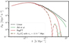Fig. 6. Models for the isotropic velocity divergence power spectrum of matter at z = 0: linear theory (black dashed), an empirical model based on fits to N-body simulations from Bel et al. (2019; green), and a beyond first-order perturbation theory model from Taruya et al. (2012; red). For these two models, we show the power spectrum with a damping function using σu = 15 h−1Mpc (dashed lines). Nonlinearities become important at k > 0.1 h Mpc−1.

3.2.4. Including observational uncertainties

The covariance matrix C(p, p_HD) has to also take into account random motions on very small scales and observational uncertainties. The random motions are modeled by a diagonal term of velocity dispersion σ_v. We also assumed that uncertainties on estimated velocities ${\sigma }_{\widehat{v},i}$ are uncorrelated. We checked in Appendix A.4 that our estimated velocities follow a Gaussian distribution. The parameter vector is p = {fσ₈, σ_v, σ_u} and the expression of the covariance matrix is

$$\begin{array}{c}\hfill C_{\mathit{ij}}(\mathbf{p},{\mathbf{p}}_{\mathrm{HD}})=C_{\mathit{ij}}^{\mathit{vv}}(f{\sigma }_8,{\sigma }_u)+[{\sigma }_v^2+{\sigma }_{\widehat{v},i}^2({\mathbf{p}}_{\mathrm{HD}})]{\delta }_{\mathit{ij}}^K,\end{array}$$(38)

where $C_{\mathit{ij}}^{\mathit{vv}}(f{\sigma }_8,{\sigma }_u)$ is given by Eq. (34) and ${\delta }_{ij}^K$ is the Kronecker delta.

3.3. Likelihood exploration

Using the data vector of peculiar velocities from Sect. 3.1 and the covariance matrix from Sect. 3.2, we proceeded to explore the likelihood (Eq. (16)) in order to constrain the growth-rate fσ₈, the velocity dispersion σ_v and the damping term σ_u.

We used the gradient descent algorithm IMINUIT¹⁰ (Dembinski et al. 2020) to find the maximum likelihood. Errors are given as symmetric errors computed with HESSE function or asymmetric errors using the MINOS function. In order to check these uncertainties evaluations and more generally the likelihood profile, we used a Markov chain Monte-Carlo (MCMC) algorithm implemented in the EMCEE¹¹ package. We fund excellent agreement between both evaluations so we mostly used the faster maximization by IMINUIT, unless stated otherwise.

4. Results

In this section, we present measurements of fσ₈ from our simulated sets of ZTF SNe Ia. As described in Sect. 2.5, the ZTF observation strategy, particularly the spectroscopic follow-up of transients for classification, introduces strong selection effects, which can lead to biases in peculiar velocities and therefore on our estimates of fσ₈. We defined a sample with limited selection effects and showed that we obtain unbiased results on fσ₈. To help identify effects on the fσ₈ fit we performed it in three different configurations, with increasing complexity: in the first, we fit p parameters using the true input velocities (i.e., no Hubble diagram fit); in the second we fit p parameters using estimated velocities but still fixing p_HD to input values; finally we fit p and p_HD parameters simultaneously. This last configuration is our baseline choice. We detail our findings in the following.

4.1. Selection effects on Hubble residuals and velocities

We started by assuming the true Tripp relation (Eq. (17)) used to build our simulation (i.e., fixing the p_HD to value of Table 2) in order to standardize the simulated SNe Ia and obtain distance moduli μ. In other words, we do not perform a fit for these values just yet as we would do in the real analysis (see next section). With this procedure we can disentangle different sources of biases to the final analysis.

Figure 7 shows the residuals to the Hubble diagram and how these residuals translate to biases in the estimated velocities. The analysis was performed on our 27 mock realizations. We can see that at redshifts above z ∼ 0.06, the Hubble diagram residuals become increasingly biased, reaching Δ_μ ≃ −0.13 at z ∼ 0.12. This is a manifestation of a selection effect (or Malmquist bias), mainly caused by the spectroscopic follow-up for typing the transients (see Sect. 2.5). We converted Hubble residuals relative to the true input Hubble diagram into peculiar velocities using Eq. (21). The bottom panel of Fig. 7 displays the comparison between estimated velocities and the true input radial velocities of the simulation. We can see that the selection bias simply translates to a fake outflow above z_obs ∼ 0.06. However, the true peculiar velocity distribution itself is not biased by these selection effects. As we said previously peculiar velocities have only a negligible effect on SN Ia magnitude, thus they are not affected by the sample bias that is mostly a magnitude cut.

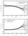Fig. 7. Hubble residuals and estimated velocities versus redshift. Top panel: Hubble residuals of the 27 mocks. The gray lines represent each mock, red points are the weighted means taken within each redshift bin. Bottom panel: same for the estimated peculiar velocities.

We can see in Fig. 7 that at z_obs = 0.02 the mean residuals seem to have a small positive bias. This effect is due to the fact that a sharp cut in z_obs leads to an asymmetric cut in velocity space: there are more hosts with higher z_cos and negative velocities that contaminate the redshift bin than lower redshift hosts with positive velocities. We checked that replacing z_obs by z_cos removes this positive bias. Nonetheless, this bias at the low-redshift end does not impact our growth rate measurements (see next section).

4.2. Growth-rate measurement forecast from the complete sample (z < 0.06)

Since Hubble residuals, and hence velocities, become strongly biased with increasing redshift, we decided to cut our sample at z_obs = 0.06 where the sample bias remains below ∼ − 0.01 mag on μ. With this cut we are left with ⟨N⟩∼1660 SNe Ia at redshift z < 0.06. We performed the measurement of the growth rate fσ₈ for the three types of analyses mentioned earlier. Results are summarized in Fig. 8 and commented below.

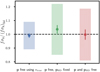Fig. 8. Best fit fσ8 for the “complete sample” within a redshift range of zobs ∈ [0.02, 0.06]. The points with errorbars show the mean obtained with our 27 mocks, the colored boxes show the averages of uncertainties.

We first fit parameters p using the true peculiar velocities from the simulation. The point on the left in Fig. 8 shows the estimation of fσ₈ from these fits for 27 mock realizations. We obtained ⟨fσ₈/(fσ₈)_fid⟩ = 0.991 ± 0.016 with an averaged uncertainty¹² of 0.100. This nonbiased result show that the model of covariance is a good description of our data. This result also set the minimum error that we can achieve with our sample if we access a perfect measurement of each velocity.

We then performed our fit using estimated velocities but fixing p_HD to input values. With these noisy velocity measurements, we observed that we do not have enough constraining power to measure σ_u. Due to positive degeneracy between the high-value of σ_u and fσ₈ we then over-estimated σ_u and fσ₈. We note here that the large values of σ_u much above the scale of redshift-space distortions are not physical. To overcome this problem, we imposed a Gaussian prior on σ_u. This prior is centered on the value of μ_p(σu) = 15 h⁻¹Mpc with a scale of σ_p(σu) = 50 percent. We chose this prior value near what has been observed in Koda et al. (2014). This is also very close to what we obtain in our fit using true velocities (⟨σ_u⟩ = 14.6 ± 0.5 h⁻¹Mpc) In Sect. 5.1 we further discuss the impact of this choice of prior. We recover ⟨fσ₈/(fσ₈)_fid⟩ = 1.036 ± 0.031 with a bias smaller than 2σ. However this bias is undetectable for one single mock realization since the average uncertainty is 0.185. This is shown in the middle of Fig. 8.

We then proceeded to a global fit letting all parameters free (p and p_HD) as one would ideally do in the analysis. Using the 6-year dataset, we verified that the fσ₈ value is not biased, as can be seen in Fig. 8.

However, on the bottom panel of Fig. 9 we can notice that one of our 27 mocks has low fit values of fσ₈ and that its fit became unstable for the smallest redshift range leading to null value of fσ₈ with extremely large errors. We checked that this mock does not give abnormal values of fσ₈ for the two previous fits (using true velocities and fixing p_HD), and that removing it from our sample does not affect significantly our results. Since its minimum is reported as valid by MINUIT we kept it in our main results. We obtained

$$\begin{array}{c}\hfill \langle f{\sigma }_8/{(f{\sigma }_8)}_{\mathrm{fid}}\rangle =0.998\pm 0.037,\end{array}$$(39)

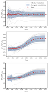Fig. 9. fσ8 fit results versus redshift cut upper bound zmax. Top panel: fit results using vtrue. Mid panel: fit results using $\widehat{v}$ with p free and pHD fixed. Bottom panel: fit results using $\widehat{v}$ with p and pHD free.

and an average uncertainty of

$$\begin{array}{c}\hfill \sqrt{\langle {\sigma }_{f{\sigma }_8}^2\rangle }/{(f{\sigma }_8)}_{\mathrm{fid}}=0.188.\end{array}$$(40)

We summarized our results on the 27 mocks in Table 4. We see that M₀ is ∼0.01 mag lower than the input value, this is what dominated the sample selection bias study in Sect. 4.1. The standardization parameters α and β are, on average, biased with respect to the input values. We have checked with a Hubble diagram fit on simulation outputs on the parent sample (before any selection) that we retrieved the true input parameters. We concluded that these biases come from selection effects but have negligible impact on fσ₈ since we do not observe a strong correlation between these parameters. The SN Ia intrinsic scattering σ_M is retrieved with good precision. To check the likelihood profile, we also ran a MCMC for one of our mocks. The corresponding posterior distributions are presented in Fig. 10. The asymmetric MINOS errors and MCMC chains analysis reveal a slightly larger upper error-bar for fσ₈. This can be explained by the degeneracy of fσ₈ with σ_u. We also observed the correlation between the intrinsic scattering σ_M and the velocity noise parameter σ_v. We can also note that σ_u constraints are dominated by our prior.

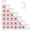Fig. 10. Posterior distributions for the joint fit (Hubble diagram and growth-rate parameters) of a single mock realization of the ZTF 6-year SN Ia program. The red contours show 1 and 2-σ levels, the dotted black lines are the true values, the dotted blue line represents the prior on σu and the green square show the MINUIT results.

4.3. Comparison with previous measurements

Our baseline analysis of the ZTF 6-years SN Ia sample yields an uncertainty of 19% on the growth rate of structures fσ₈ (Eq. (40)) when considering the ⟨N⟩∼1660 SNe Ia distributed over more than 28k deg² and 0.02 < z < 0.06. We considered only velocity-velocity correlations in this work. It is interesting to compare our predictions to past measurements of fσ₈ using peculiar velocity data.

Figure 11 compares our estimate from ZTF simulations to previous measurements, all of them using Tully-Fisher or Fundamental Plane distances (except Johnson et al. 2014; Boruah et al. 2020 who include SNe Ia from several compilations). Most datasets also include a galaxy survey in order to cross-correlate density and velocity field, so their information source is larger than in our case where we just use velocities. We also make the distinction between methods (maximum-likelihood, compressed 2-pt statistics and reconstruction-based) since in principle they do not use the same amount of information from the data.

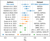Fig. 11. Measurements of the growth-rate of structures fσ8 from peculiar velocity and galaxy survey data. Error bars with lighter shade are those including quoted systematic errors (except for Dupuy et al. 2019, where the extra contribution is from cosmic variance). Our prediction is from Eq. (40) and only considers the spectroscopically classified sample of ZTF SNe Ia between 0.02 < z < 0.06.

Our result has similar constraining power to those measurements that use only peculiar velocity data (and not density) and the similar methodology as ours, such as Johnson et al. (2014), Howlett et al. (2017b), who obtain 15 and 16% respectively. Johnson et al. (2014) used 8896 FP distances from the 6dFGS between 0 < z < 0.05 (southern sky only) and 303 SNe Ia (heterogeneously distributed over the full sky). Howlett et al. (2017b) used 2062 TF distances between 0.002 < z < 0.03, which is half the span in our sample. There are slight differences in analysis choices such as the values for k_max in the evaluation of the model, or the assignment of tracers to a mesh, which we do not use.

We expect constraints to improve when combining ZTF SNe Ia with an overlapping galaxy survey. A great candidate is the DESI Bright Galaxy Survey (Hahn et al. 2023) which has large area and redshift overlap with ZTF.

5. Robustness tests and alternative forecasts

In this section we study how our results are affected when we vary the prior on σ_u or when we change the power spectrum model. We also present the expected precision for 30 months of data as well as when we include information beyond our complete sample cut at z = 0.06.

5.1. Impact of σ_u prior parameters on fσ₈

In our analysis, the σ_u parameter is responsible for a loss of the constraining power and its degeneracy with fσ₈ can lead to biased results. Some recent work (Lai et al. 2023; Howlett et al. 2022) proposed to fix this parameter with a simulation-based value. In our analysis, we chose to use a Gaussian prior. Here we evaluate the impact of this choice on the estimated fσ₈.

The top panel of Fig. 12 shows the evolution of the fσ₈ result as a function of the central value of the Gaussian σ_u prior. Between a central value of 5 to 25 h⁻¹Mpc, we get a variation of fσ₈ from ∼ − 9 to ∼ + 6 percent with respect to our baseline fit. In Koda et al. (2014), σ_u is found, using N-body simulations, within the range of [13, 15] h⁻¹Mpc. In this range we found a less than ∼2% variation of fσ₈. This result has to be mitigated since Howlett et al. (2017b) found a value of ${\sigma }_u=6.{75}_{-6.75}^{+1.74}$h⁻¹Mpc on 2MTF data and Lai et al. (2023) found that a σ_u within [19, 23] h⁻¹Mpc better match their mocks. The bottom of Fig. 12 shows the evolution of the fσ₈ result as a function of the scale of the Gaussian σ_u prior. We found that our results are insensitive to the width of this prior.

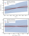Fig. 12. Effect of the σu prior on the fσ8 fit results. Top panel: evolution of the difference between fσ8 fit value and our baseline (σp(σu) = 50%) in function of the central value of the Gaussian prior on σu. The width of the prior is fixed to σp(σu) = 10 h−1Mpc. Bottom panel: evolution of the difference between fσ8 fit value and our baseline (σp(σu) = 50%). The central value of the prior is fixed to μp(σu) = 15 h−1Mpc. We use the estimated velocities of the 6-year sample.

5.2. Effect of the power spectrum model

The power spectrum from Bel et al. (2019) used in the previous section comes from a fit on N-body simulations. We checked the impact of this choice using the RegPT power-spectrum model. We performed the same fit as in Sect. 4.2 using true velocities but including all our SNe Ia up to z = 0.13 since the true velocities are not biased. We found with our 27 mocks a mean difference of ⟨Δfσ₈⟩/(fσ₈)_fid = ( − 1.5 ± 4.9)×10⁻⁴. This difference is negligible. This is expected since the overall integral of these two power-spectra only differs by less than ∼1% with σ_u = 15 h⁻¹Mpc.

We also performed a fit using the linear power spectrum. We found a difference of ⟨Δfσ₈⟩/(fσ₈)_fid = ( − 2.7 ± 0.06)×10⁻². This difference comes from the fact that the linear power spectrum overestimates the power on small scales resulting in a variance overestimation. However this bias is small and nondetectable compared to the expected uncertainty of one realization.

5.3. ZTF DR2 forecast

The next data release for ZTF (DR2) is expected to publish supernovae lightcurves for a survey of thirty-months. We simulated this sample. The statistics available after all our cuts is on average ⟨N⟩ ∼ 775 SNe Ia for our 27 mocks. From the fit with p_HD fixed we obtained ⟨fσ₈/(fσ₈)_fid⟩ = 0.968 ± 0.046, with an average uncertainty on fσ₈ of 0.246. This result is compatible with the fiducial value. When fitting with p and p_HD free, we obtained on average ⟨fσ₈/(fσ₈)_fid⟩ = 0.923 ± 0.051, at ∼1.5σ from the fiducial value. This small bias can be explained by the fact that, as seen in the third paragraph of Sect. 4.2, this fit can become unstable, due to a combination of low number of SNIa and the large number of free parameters. For the DR2 samples, a larger fraction of realizations yield excessively low values for fσ₈. This would indicate that the distribution of fσ₈ becomes non-Gaussian at such low number density of tracers. For a work on real data, this point would need further investigation. However, this bias is still negligible compared to the averaged uncertainty on fσ₈ of about 0.255. Since the number of SNe Ia is approximately divided by ∼2 within the same volume we observe the expected $\sqrt{N}$ law as $0.255\sim 0.188\times \sqrt{2}$.

5.4. Impact of a bias correction beyond z = 0.06

With our cut at z = 0.06, we are left with ⟨N⟩∼1660 SNe Ia. This number represents only half of the spectroscopically typed sample. In Fig. 9 we show fσ₈ results as a function of the redshift upper bound z_max. In the middle and bottom panel of Fig. 9, we show the impact of this sample bias on the fσ₈ fit compared to the fit using true velocities of the top pannel. After z > 0.06 the bias begins to grow up to ∼180 percent at z = 0.12.

This bias cannot be corrected simply by using the methods introduced in Betoule et al. (2014) or in Kessler & Scolnic (2017). A correction in redshift bins will shift the velocity of an entire redshift shell with the same factor, leading to fake velocity correlation.

Although we do not propose a method to actually make the correction, we explored how much we could improve the fσ₈ measurement. In what follows, we assume that we can perfectly correct for selection biases and construct an unbiased sample following two steps. First we take the velocity uncertainties ${\sigma }_{\widehat{v},i}$ of the selected sample. Then, we draw new velocities from a Gaussian distribution centered on v_true, i with standard deviation of ${\sigma }_{\widehat{v},i}$.

With this new sample of artificially corrected SN Ia velocities, we fit for fσ₈ extending the range in redshift. Results are shown in Fig. 13. We obtained for z < 0.06 (⟨N_SN⟩ = 1660) a result of ⟨fσ₈/(fσ₈)_fid⟩ = 0.994 ± 0.027, with an averaged uncertainty of 0.173 and for z < 0.13 (⟨N_SN⟩ = 3520) (i.e., a statistic multiplied by ∼2) a result of ⟨fσ₈/(fσ₈)_fid⟩ = 0.995 ± 0.024, with an averaged uncertainty of 0.148. We see that the uncertainties on fσ₈ only decrease from 17 to 15 percent when including SNe Ia with redshifts z_obs > 0.06. This can be explained by two effects: Firstly, when going deeper in redshift, the observed volume increases faster than the number of SNe Ia which at some point also decreases due to sample selection. Thus the density decreases quickly, as we shown on bottom panel of Fig. 4. Secondly, the errors on peculiar velocities increase with redshift as stated in Eq. (23). These two effects result in a reduced constraining power from SNe Ia at z > 0.06.

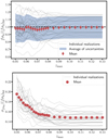Fig. 13. fσ8 constraints as a function of the upper bound in the redshift range zmax, using an artificially perfect correction for the bias on the velocities. The top panel shows the best-fit values and the bottom panel its uncertainties. Gray lines represent each mock, red points are average of 27 realizations.

6. Conclusions

In this paper we have presented detailed simulations of ZTF SN Ia samples equivalent to 6 years of data. We used these simulations to study the measurement of the growth rate of structures fσ₈ from the clustering of SN Ia peculiar velocities.

Our simulations aim to faithfully reproduce real observations, including several features: peculiar velocities and positions of host galaxies drawn from an N-body simulation, lightcurve sampling using actual ZTF metadata, realistic fluxes and uncertainties, and selection effects from photometric detection and spectroscopic follow-up for typing. We used the SALT2 model to adjust SN Ia light-curve parameters on the measurements and applied quality cuts to reproduce cosmological samples.

We have then presented the methodology proposed to derive peculiar velocities from SN Ia distances and measure the growth rate. We used the commonly employed maximum-likelihood method, which assumes the peculiar velocity field to be a multivariate Gaussian random field. The covariance matrix used in the likelihood is a function of the growth rate parameter plus SN Ia standardization and nuisance parameters. Our baseline choice of analysis fits for all parameters at once. We showed that all our results are robust against variations of the main assumptions of our analysis.

Our simulations showed that selection effects, mainly the one imposed by the spectroscopic typing, create a bias in distance estimates at z_obs > 0.06. Biases in distances translate to biases in the estimates of peculiar velocities and thus on the measurements of the growth rate.

We defined an unbiased sample of SNe Ia by considering only those at z_obs < 0.06 with which we derive constraints on fσ₈. Using the equivalent of 6-years of ZTF data and our baseline analysis settings, we showed that we can obtain unbiased estimates of fσ₈ with a 19% precision. This precision is comparable to previous measurements on data using peculiar velocity samples derived from the Fundamental Plane or the Tully-Fisher relations. Our result showcases the great potential of using SN Ia distances alone for growth-rate measurements.

Since selection effects significantly reduce the SN Ia sample size, we investigated the gain in applying a bias correction to SNe Ia at z_obs > 0.06. Assuming an artificially perfect bias correction and using the full available redshift range of spectroscopically typed SNe Ia our constraints on fσ₈ reduce from 17 to 15%. This small improvement is mainly due to the rapid decrease in comoving density of tracers between 0.06 < z < 0.10 and the increase in the velocity uncertainties due to intrinsic scatter of SN Ia peak brightness. Significant improvement could be expected by using a photometrically typed sample of SNe Ia which is larger and push the decline of the comoving density to a higher redshift. We leave this investigation for future work.

The work of this paper sets the basis for the measurement of the growth rate with real ZTF data. The same methodologies can be applied to SN Ia samples from the Vera Rubin Observatory, where spectroscopic follow-up cannot be performed and measurements will rely on photometric typing.

Acknowledgments

Simulation logs are based on observations obtained with the Samuel Oschin Telescope 48-inch and the 60-inch Telescope at the Palomar Observatory as part of the Zwicky Transient Facility project. ZTF is supported by the National Science Foundation under Grants No. AST-1440341 and AST-2034437 and a collaboration including current partners Caltech, IPAC, the Weizmann Institute of Science, the Oskar Klein Center at Stockholm University, the University of Maryland, Deutsches Elektronen-Synchrotron and Humboldt University, the TANGO Consortium of Taiwan, the University of Wisconsin at Milwaukee, Trinity College Dublin, Lawrence Livermore National Laboratories, IN2P3, University of Warwick, Ruhr University Bochum, Northwestern University and former partners the University of Washington, Los Alamos National Laboratories, and Lawrence Berkeley National Laboratories. Operations are conducted by COO, IPAC, and UW. The project leading to this publication has received funding from Excellence Initiative of Aix-Marseille University-A*MIDEX, a French “Investissements d’Avenir” program (AMX-20-CE-02-DARKUNI). Some of the results in this paper have been derived using the healpy and HEALPix packages.

References

Appendix A: Peculiar velocity estimators

A.1. Derivation of the peculiar velocity estimator

Hubble residuals are given as

$$\begin{array}{c}\hfill \mathrm{\Delta }\mu ={\mu }_{\mathrm{obs}}-{\mu }_{\mathrm{model}}(z_{\mathrm{obs}}),\end{array}$$(A.1)

where μ_model expression is

$$\begin{array}{c}\hfill {\mu }_{\mathrm{model}}(z)=5log\left(d_{L,\mathrm{model}}(z)\right)=5log((1+z)r(z)),\end{array}$$(A.2)

with r(z) the comoving distance. In the residuals, μ_model(z) is evaluated at z = z_obs = (1 + z_p)(1 + z_cos)−1.

The first-order Taylor’s expansion of d_L, model(z_obs) with respect to z_p is

$$\begin{array}{c}\hfill d_{L,\mathrm{model}}(z_{\mathrm{obs}})\simeq d_{L,\mathrm{model}}(z_{\cos })+{\frac{\partial z}{\partial z_p}\frac{\partial d_{L,\mathrm{th}}}{\partial z}|}_{z_p=0}{z}_p.\end{array}$$(A.3)

We can develop the second term of (A.3)

$$\begin{array}{cc}\hfill {\frac{\partial z}{\partial z_p}\frac{\partial d_{L,\mathrm{th}}}{\partial z}|}_{z_p=0}& \simeq (1+z_{\cos })\hfill \\ \hfill & \times \frac{\partial }{\partial z}{\left[(1+z)\frac{c}{H_0}{\displaystyle {\int }_0^z}\frac{d{z}^{\prime }}{E(z^{\prime })}\right]|}_{z_p=0}\hfill \\ \hfill & \simeq (1+z_{\cos })\hfill \\ \hfill & \times (\frac{c}{H_0}{\displaystyle {\int }_0^{z_{\cos }}}\frac{d{z}^{\prime }}{E(z^{\prime })}+\frac{c(1+z_{\cos })}{H_{0}E(z_{\cos })})\hfill \\ \hfill & \simeq (1+z_{\cos })(r(z_{\cos })+\frac{c{(1+z_{\cos })}^2}{H(z_{\cos })})\hfill \\ \hfill & \simeq d_{L,\mathrm{model}}(z_{\cos })(1+\frac{c(1+z_{\cos })}{r(z_{\cos })H(z_{\cos })}).\hfill \end{array}$$(A.4)

Injecting (A.4) in (A.3) we obtain

$$\begin{array}{cc}\hfill d_{L,\mathrm{model}}(z_{\mathrm{obs}})& \simeq d_{L,\mathrm{model}}(z_{\cos })\hfill \\ \hfill & \times [1+(1+\frac{c(1+z_{\cos })}{r(z_{\cos })H(z_{\cos })})z_p],\hfill \end{array}$$

where d_L, model(z_cos) can be replaced by $\frac{d_{L,\mathrm{obs}}}{{(1+z_p)}^2}$ to give

$$\begin{array}{cc}\hfill d_{L,\mathrm{model}}(z_{\mathrm{obs}})& \simeq \frac{d_{L,\mathrm{obs}}}{{(1+z_p)}^2}[1+(1+\frac{c(1+z_{\cos })}{r(z_{\cos })H(z_{\cos })})z_p]\hfill \\ \hfill & \simeq d_{L,\mathrm{obs}}[1+(\frac{c(1+z_{\cos })}{r(z_{\cos })H(z_{\cos })}-1)z_p].\hfill \end{array}$$(A.5)

With (A.5) we can write the relative variation of luminosity distances

$$\begin{array}{c}\hfill \delta d_L=\frac{d_{L,\mathrm{obs}}-d_{L,\mathrm{model}}(z_{\mathrm{obs}})}{d_{L,\mathrm{model}}(z_{\mathrm{obs}})}\simeq (1-\frac{c(1+z_{\cos })}{r(z_{\cos })H(z_{\cos })})z_p.\end{array}$$(A.6)

This last equation is equivalent to the Eq. 15 from Hui & Greene (2006). Using $\mathrm{\Delta }\mu \simeq \frac{5}{ln(10)}\delta d_L$ and v_p ≃ cz_p we finally get

$$\begin{array}{c}\hfill v_p\simeq -\frac{ln(10)c}{5}{(\frac{c(1+z_{\cos })}{r(z_{\cos })H(z_{\cos })}-1)}^{-1}\mathrm{\Delta }\mu .\end{array}$$(A.7)

As a first order development, this derivation is valid for velocities such that z_p is small compared to z_cos. In Appendix A.2 we discuss further approximations and biases of this estimator.

A.2. The different estimators and their bias

In the literature we can find variants of the peculiar velocity estimator (21):

$$\begin{array}{c}\hfill {\widehat{v}}_1=-\frac{ln(10)c}{5}{(\frac{(1+z_{\cos })c}{H(z_{\cos })r(z_{\cos })}-1)}^{-1}\mathrm{\Delta }\mu .\end{array}$$(A.8)

Here we describe which approximations are made and their consequences on peculiar velocity estimation. From ${\widehat{v}}_1$ we can make two approximations. Firstly, since $\frac{(1+z_{\cos })c}{H(z_{\cos })r(z_{\cos })}>10$ for z < 0.11 at low-redshift we can make the approximation:

$$\begin{array}{c}\hfill {\widehat{v}}_2=-\frac{ln(10)c}{5}\frac{H(z_{\cos })r(z_{\cos })}{1+z_{\cos }}\mathrm{\Delta }\mu .\end{array}$$(A.9)

The form (A.9) is used in Howlett et al. (2017b), Huterer et al. (2017) and Lai et al. (2023). Secondly, at the low-redshift regime we can also approximate the Hubble law

$$\begin{array}{c}\hfill H(z_{\cos })r(z_{\cos })\simeq c{z}_{\mathrm{mod}},\end{array}$$(A.10)

where cz_mod is a development of the Hubble law at a given order. Here, we use the first order development cz_mod = cz_cos¹³, then (21) becomes:

$$\begin{array}{c}\hfill {\widehat{v}}_3=-\frac{ln(10)c}{5}{(\frac{1+z_{\cos }}{z_{\mathrm{mod}}}-1)}^{-1}\mathrm{\Delta }\mu .\end{array}$$(A.11)

Using those approximations together, we obtain:

$$\begin{array}{c}\hfill {\widehat{v}}_4=-\frac{ln(10)c}{5}\frac{z_{\mathrm{mod}}}{1+z_{\cos }}\mathrm{\Delta }\mu .\end{array}$$(A.12)

This last estimator corresponds to the Watkins estimator Watkins & Feldman (2015).

As we have seen in Appendix A.1, the derivation of these estimators make the assumption that z_p is small enough compared to z_cos. This statement tends to be less valid at very low redshift when z_cos is of the same order of magnitude than z_p. Moreover we stated in Sect. 3.1.2 that we can not have access to the cosmological redshift z_cos, hence we need to evaluate our estimator using the observed redshift z_obs. On Fig. A.1, we see in the upper left panel, that these approximations leads to a biased velocity estimation especially at very low redshift z < 0.02 where the bias magnitude for a velocity of v ∼ 300 km/s is above ∼5% for ${\widehat{v}}_1$. Comparing the estimators, we see that neglecting the "-1" term as in ${\widehat{v}}_2$ and ${\widehat{v}}_4$, leads to a global velocity underestimation when the redshift increases. Using the linear approximation of the Hubble law, used in ${\widehat{v}}_3$, also tends to give underestimated velocities compared to using the real Hubble law. The first approximation is the dominant effect on the bias for the combined approximation of the ${\widehat{v}}_4$ estimator.

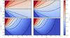Fig. A.1. Bias on velocity estimator as a function of cosmological redshift (zcos ∈ [0.005, 0.12]) and true velocity. Upper left panel: ${\widehat{v}}_1$ estimator. Bottom left panel: ${\widehat{v}}_2$ estimator. Upper right panel: ${\widehat{v}}_3$ estimator. Bottom right panel: ${\widehat{v}}_4$ estimator. See discussion in Appendix A.2.

A.3. Estimator dependence on Ω_m assumptions

Using the Hubble law in our estimator, we have to fix a cosmology, Ω_m in Flat-ΛCDM. Using a Ω_m that differs from the true cosmology leads to a biased estimation of velocities. In Fig. A.2 we show the bias for a velocity fixed to v_true = 300 km.s⁻¹ as a function of the Ω_m assumption and redshift z_cos. As previously stated, biases at low-redshift are dominated by the loss of accuracy of the first order development when z_cos ∼ z_p. The bias due to the mis-estimation of Ω_m appears with increasing redshift. However with the current precision of Ω_m from Planck Collaboration VI (2020) of ∼2% the bias stays below 5% for redshifts z < 0.06.

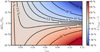Fig. A.2. Bias on velotity estimator ${\widehat{v}}_1$ as a function of cosmological redshift and Ωm used in the estimator. The true velocity is fixed to vtrue = 300 km.s−1. See discussion in A.3.

A.4. Estimators Gaussianity

The likelihood we used to estimate fσ₈ assumes that the velocity estimator has a Gaussian distribution. We have to check that the estimator preserves the Gaussian form of the errors on Δμ. In order to check this, we used a "toy model". We drew N peculiar velocities from a normal distribution v_p ∼ 𝒩(0, 300) as well as N cosmological redshifts. After computing μ_obs using (8) we add a Gaussian scattering with σ_μ ∼ 𝒩(0, 0.12).

In the top panel of Fig. A.3, we can see that the pull of the velocity estimator ${\widehat{v}}_1$ seems to preserve the Gaussian distribution of σ_μ for redshift range z ∈ [0.02, 0.06]. In the bottom panel of Fig. A.3, we see that below z < 0.02 the velocity distribution deviates from Gaussianity due to more important effect from peculiar velocity redshift contamination.

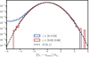Fig. A.3. Pull of peculiar velocity estimator for ${\widehat{v}}_1$ on a "toy model" drawing N = 106 SNe Ia. The blue line represents the pull for SNe Ia in the redshift range [0, 0.02] and the red line represents the pull for SNe Ia in the redshift range [0.02, 0.06]. We see that for low redshift SNe Ia the velocity estimator deviates from Gaussianity due to peculiar velocity contamination of zobs.

Appendix B: Power spectrum convergence

As stated in Sect. 3.2.2 we chose the integration limit of the power spectrum such as the integral has converged. In Fig. B.1 we show the integral of the power spectrum as a function of the k_max upper bound of integration normalized by the integral with k_max = 10h Mpc⁻¹. At k_max = 1h Mpc⁻¹ we see that the integral has converged.

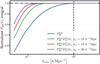Fig. B.1. Normalized integral of the power spectrum as a funtion of integration upper bound kmax.

All Tables

All Figures

Fig. 1. Toy model illustrating how peculiar velocities impact the observed redshift zobs and the observed distance moduli μobs. Radial peculiar velocities are randomly drawn from a Gaussian distribution with σvp = 300 km s−1. The color of each point indicates the value of its radial peculiar velocities vp. The effect on the x-axis is of first order on vp while the effect on the y-axis is of second order.

In the text

	Fig. 2. Examples of simulated ZTF light-curves of type-Ia supernovae at low, intermediate and high redshifts. Points with error bars are the simulated data, and the solid lines are the input light-curves.
In the text

Fig. 3. Angular distribution and completeness of the simulated ZTF SN Ia sample. Top: angular distribution of simulated ZTF type-Ia supernova from one mock realization of a 6-year program. The parent sample of simulated SNe Ia is shown in blue, those detected in photometry are shown in green and those successfully typed with spectroscopy are shown in red. A map of stellar density from the Gaia satellite is shown in the background. Bottom: angular completeness of photometric (left) and spectroscopic samples (right). The photometric completeness is computed relative to the parent sample while the spectroscopic one is relative to those detected in photometry, using the full redshift range of the simulation, that is 0 < z < 0.14. Different ranges are used for the color scales.

In the text

Fig. 4. Number and density distributions of SNe Ia with respect to redshift. The parent sample of simulated SNe Ia is shown in blue, those detected in photometry are shown in green and those successfully typed with spectroscopy are shown in red. Top panel: number of simulated ZTF type-Ia supernova versus redshift per bins of Δzobs = 0.005, averaged over 27 independent mock realizations of a 6-year program. Bottom panel: comoving number density of SNe Ia versus redshift, calculated assuming the fiducial cosmology from Table 1.

In the text

	Fig. 5. Representation of the different effects of peculiar velocities on the Hubble diagram for a single SN. The red dotted line shows the Doppler shift, the yellow line shows the relativistic beaming effect and the green dotted line shows the Hubble residual.
In the text

Fig. 6. Models for the isotropic velocity divergence power spectrum of matter at z = 0: linear theory (black dashed), an empirical model based on fits to N-body simulations from Bel et al. (2019; green), and a beyond first-order perturbation theory model from Taruya et al. (2012; red). For these two models, we show the power spectrum with a damping function using σu = 15 h−1Mpc (dashed lines). Nonlinearities become important at k > 0.1 h Mpc−1.

In the text

	Fig. 7. Hubble residuals and estimated velocities versus redshift. Top panel: Hubble residuals of the 27 mocks. The gray lines represent each mock, red points are the weighted means taken within each redshift bin. Bottom panel: same for the estimated peculiar velocities.
In the text

	Fig. 8. Best fit fσ8 for the “complete sample” within a redshift range of zobs ∈ [0.02, 0.06]. The points with errorbars show the mean obtained with our 27 mocks, the colored boxes show the averages of uncertainties.
In the text

	Fig. 9. fσ8 fit results versus redshift cut upper bound zmax. Top panel: fit results using vtrue. Mid panel: fit results using $\widehat{v}$ with p free and pHD fixed. Bottom panel: fit results using $\widehat{v}$ with p and pHD free.
In the text

	Fig. 10. Posterior distributions for the joint fit (Hubble diagram and growth-rate parameters) of a single mock realization of the ZTF 6-year SN Ia program. The red contours show 1 and 2-σ levels, the dotted black lines are the true values, the dotted blue line represents the prior on σu and the green square show the MINUIT results.
In the text

	Fig. 11. Measurements of the growth-rate of structures fσ8 from peculiar velocity and galaxy survey data. Error bars with lighter shade are those including quoted systematic errors (except for Dupuy et al. 2019, where the extra contribution is from cosmic variance). Our prediction is from Eq. (40) and only considers the spectroscopically classified sample of ZTF SNe Ia between 0.02 < z < 0.06.
In the text

Fig. 12. Effect of the σu prior on the fσ8 fit results. Top panel: evolution of the difference between fσ8 fit value and our baseline (σp(σu) = 50%) in function of the central value of the Gaussian prior on σu. The width of the prior is fixed to σp(σu) = 10 h−1Mpc. Bottom panel: evolution of the difference between fσ8 fit value and our baseline (σp(σu) = 50%). The central value of the prior is fixed to μp(σu) = 15 h−1Mpc. We use the estimated velocities of the 6-year sample.

In the text

	Fig. 13. fσ8 constraints as a function of the upper bound in the redshift range zmax, using an artificially perfect correction for the bias on the velocities. The top panel shows the best-fit values and the bottom panel its uncertainties. Gray lines represent each mock, red points are average of 27 realizations.
In the text

	Fig. A.1. Bias on velocity estimator as a function of cosmological redshift (zcos ∈ [0.005, 0.12]) and true velocity. Upper left panel: ${\widehat{v}}_1$ estimator. Bottom left panel: ${\widehat{v}}_2$ estimator. Upper right panel: ${\widehat{v}}_3$ estimator. Bottom right panel: ${\widehat{v}}_4$ estimator. See discussion in Appendix A.2.
In the text

	Fig. A.2. Bias on velotity estimator ${\widehat{v}}_1$ as a function of cosmological redshift and Ωm used in the estimator. The true velocity is fixed to vtrue = 300 km.s−1. See discussion in A.3.
In the text

Fig. A.3. Pull of peculiar velocity estimator for ${\widehat{v}}_1$ on a "toy model" drawing N = 106 SNe Ia. The blue line represents the pull for SNe Ia in the redshift range [0, 0.02] and the red line represents the pull for SNe Ia in the redshift range [0.02, 0.06]. We see that for low redshift SNe Ia the velocity estimator deviates from Gaussianity due to peculiar velocity contamination of zobs.

In the text

	Fig. B.1. Normalized integral of the power spectrum as a funtion of integration upper bound kmax.
In the text

References

- Abate, A., Bridle, S., Teodoro, L. F. A., Warren, M. S., & Hendry, M. 2008, MNRAS, 389, 1739 [NASA ADS] [CrossRef] [Google Scholar]
- Adams, C., & Blake, C. 2020, MNRAS, 494, 3275 [NASA ADS] [CrossRef] [Google Scholar]
- Alam, S., Aubert, M., Avila, S., et al. 2021, Phys. Rev. D, 103, 083533 [NASA ADS] [CrossRef] [Google Scholar]
- Avila, S., Gonzalez-Perez, V., Mohammad, F. G., et al. 2020, MNRAS, 499, 5486 [NASA ADS] [CrossRef] [Google Scholar]
- Barbary, K., Bailey, S., Barentsen, G., et al. 2016, https://doi.org/10.5281/zenodo.592747 [Google Scholar]
- Bautista, J. E., Paviot, R., Vargas Magaña, M., et al. 2021, MNRAS, 500, 736 [Google Scholar]
- Bel, J., Pezzotta, A., Carbone, C., Sefusatti, E., & Guzzo, L. 2019, A&A, 622, A109 [NASA ADS] [CrossRef] [EDP Sciences] [Google Scholar]
- Bellm, E. C., Kulkarni, S. R., Barlow, T., et al. 2019, PASP, 131, 068003 [Google Scholar]
- Betoule, M., Kessler, R., Guy, J., et al. 2014, A&A, 568, A22 [NASA ADS] [CrossRef] [EDP Sciences] [Google Scholar]
- Beutler, F., Blake, C., Colless, M., et al. 2012, MNRAS, 423, 3430 [NASA ADS] [CrossRef] [Google Scholar]
- Beutler, F., Seo, H.-J., Saito, S., et al. 2017, MNRAS, 466, 2242 [Google Scholar]
- Blake, C., Brough, S., Colless, M., et al. 2011, MNRAS, 415, 2876 [NASA ADS] [CrossRef] [Google Scholar]
- Boruah, S. S., Hudson, M. J., & Lavaux, G. 2020, MNRAS, 498, 2703 [Google Scholar]
- Boruah, S. S., Lavaux, G., & Hudson, M. J. 2022, MNRAS, 517, 4529 [NASA ADS] [CrossRef] [Google Scholar]
- Cardelli, J. A., Clayton, G. C., & Mathis, J. S. 1989, ApJ, 345, 245 [Google Scholar]
- Carrick, J., Turnbull, S. J., Lavaux, G., & Hudson, M. J. 2015, MNRAS, 450, 317 [Google Scholar]
- Clifton, T., Ferreira, P. G., Padilla, A., & Skordis, C. 2012, Phys. Rep., 513, 1 [NASA ADS] [CrossRef] [Google Scholar]
- Dam, L., Bolejko, K., & Lewis, G. F. 2021, JCAP, 2021, 018 [CrossRef] [Google Scholar]
- Davis, M., Nusser, A., Masters, K. L., et al. 2011a, MNRAS, 413, 2906 [Google Scholar]
- Davis, T. M., Hui, L., Frieman, J. A., et al. 2011b, ApJ, 741, 67 [NASA ADS] [CrossRef] [Google Scholar]
- Dekany, R., Smith, R. M., Riddle, R., et al. 2020, PASP, 132, 038001 [NASA ADS] [CrossRef] [Google Scholar]
- de la Torre, S., Jullo, E., Giocoli, C., et al. 2017, A&A, 608, A44 [NASA ADS] [CrossRef] [EDP Sciences] [Google Scholar]
- de Mattia, A., Ruhlmann-Kleider, V., Raichoor, A., et al. 2021, MNRAS, 501, 5616 [NASA ADS] [Google Scholar]
- Dembinski, H., Ongmongkolkul, P., Deil, C., et al. 2020, https://doi.org/10.5281/zenodo.3949207 [Google Scholar]
- Dhawan, S., Goobar, A., Smith, M., et al. 2022, MNRAS, 510, 2228 [NASA ADS] [CrossRef] [Google Scholar]
- Djorgovski, S., & Davis, M. 1987, ApJ, 313, 59 [Google Scholar]
- Dupuy, A., Courtois, H. M., & Kubik, B. 2019, MNRAS, 486, 440 [NASA ADS] [CrossRef] [Google Scholar]
- Ezquiaga, J. M., & Zumalacárregui, M. 2018, Front. Astron. Space Sci., 5, 44 [NASA ADS] [CrossRef] [Google Scholar]
- Feindt, U., Nordin, J., Rigault, M., et al. 2019, JCAP, 10, 005 [CrossRef] [Google Scholar]
- Fremling, C., Miller, A. A., Sharma, Y., et al. 2020, ApJ, 895, 32 [NASA ADS] [CrossRef] [Google Scholar]
- Gil-Marín, H., Guy, J., Zarrouk, P., et al. 2018, MNRAS, 477, 1604 [Google Scholar]
- Gil-Marín, H., Bautista, J. E., Paviot, R., et al. 2020, MNRAS, 498, 2492 [Google Scholar]
- Gorski, K. M., Davis, M., Strauss, M. A., White, S. D. M., & Yahil, A. 1989, ApJ, 344, 1 [NASA ADS] [CrossRef] [Google Scholar]
- Górski, K. M., Hivon, E., Banday, A. J., et al. 2005, ApJ, 622, 759 [Google Scholar]
- Graham, M. J., Kulkarni, S. R., Bellm, E. C., et al. 2019, PASP, 131, 078001 [Google Scholar]
- Grieb, J. N., Sánchez, A. G., Salazar-Albornoz, S., et al. 2017, MNRAS, 467, 2085 [NASA ADS] [Google Scholar]
- Guy, J., Astier, P., Baumont, S., et al. 2007, A&A, 466, 11 [NASA ADS] [CrossRef] [EDP Sciences] [Google Scholar]
- Guy, J., Sullivan, M., Conley, A., et al. 2010, A&A, 523, A7 [NASA ADS] [CrossRef] [EDP Sciences] [Google Scholar]
- Guzzo, L., Pierleoni, M., Meneux, B., et al. 2008, Nature, 451, 541 [Google Scholar]
- Hahn, C., Wilson, M. J., Ruiz-Macias, O., et al. 2023, AJ, 165, 253 [CrossRef] [Google Scholar]
- Heitmann, K., Finkel, H., Pope, A., et al. 2019, ApJS, 245, 16 [NASA ADS] [CrossRef] [Google Scholar]
- Hou, J., Sánchez, A. G., Scoccimarro, R., et al. 2018, MNRAS, 480, 2521 [NASA ADS] [CrossRef] [Google Scholar]
- Hou, J., Sánchez, A. G., Ross, A. J., et al. 2021, MNRAS, 500, 1201 [Google Scholar]
- Howlett, C., Ross, A. J., Samushia, L., Percival, W. J., & Manera, M. 2015, MNRAS, 449, 848 [NASA ADS] [CrossRef] [Google Scholar]
- Howlett, C., Staveley-Smith, L., Elahi, P. J., et al. 2017a, MNRAS, 471, 3135 [NASA ADS] [CrossRef] [Google Scholar]
- Howlett, C., Robotham, A. S. G., Lagos, C. D. P., & Kim, A. G. 2017b, ApJ, 847, 128 [NASA ADS] [CrossRef] [Google Scholar]
- Howlett, C., Said, K., Lucey, J. R., et al. 2022, MNRAS, 515, 953 [NASA ADS] [CrossRef] [Google Scholar]
- Hui, L., & Greene, P. B. 2006, Phys. Rev. D, 73, 123526 [NASA ADS] [CrossRef] [Google Scholar]
- Huterer, D., Shafer, D. L., Scolnic, D. M., & Schmidt, F. 2017, JCAP, 2017, 015 [CrossRef] [Google Scholar]
- Johnson, A., Blake, C., Koda, J., et al. 2014, MNRAS, 444, 3926 [NASA ADS] [CrossRef] [Google Scholar]
- Kessler, R., & Scolnic, D. 2017, ApJ, 836, 56 [Google Scholar]
- Kim, A. G., & Linder, E. V. 2020, Phys. Rev. D, 101, 023516 [NASA ADS] [CrossRef] [Google Scholar]
- Koda, J., Blake, C., Davis, T., et al. 2014, MNRAS, 445, 4267 [NASA ADS] [CrossRef] [Google Scholar]
- Lai, Y., Howlett, C., & Davis, T. M. 2023, MNRAS, 518, 1840 [Google Scholar]
- Lewis, A., Challinor, A., & Lasenby, A. 2000, ApJ, 538, 473 [Google Scholar]
- LSST Science Collaboration (Abell, P. A., et al.) 2009, ArXiv e-prints [arXiv:0912.0201] [Google Scholar]
- Lyall, S., Blake, C., Turner, R., Ruggeri, R., & Winther, H. 2022, MNRAS, 518, 5929 [NASA ADS] [CrossRef] [Google Scholar]
- Ma, Y.-Z., Gordon, C., & Feldman, H. A. 2011, Phys. Rev. D, 83, 103002 [NASA ADS] [CrossRef] [Google Scholar]
- Masci, F. J., Laher, R. R., Rusholme, B., et al. 2019, PASP, 131, 018003 [Google Scholar]
- Neveux, R., Burtin, E., de Mattia, A., et al. 2020, MNRAS, 499, 210 [NASA ADS] [CrossRef] [Google Scholar]
- Nicolas, N., Rigault, M., Copin, Y., et al. 2021, A&A, 649, A74 [NASA ADS] [CrossRef] [EDP Sciences] [Google Scholar]
- Nusser, A. 2017, MNRAS, 470, 445 [NASA ADS] [CrossRef] [Google Scholar]
- Okumura, T., Hikage, C., Totani, T., et al. 2016, PASJ, 68, 38 [NASA ADS] [Google Scholar]
- Perley, D. A., Fremling, C., Sollerman, J., et al. 2020, ApJ, 904, 35 [NASA ADS] [CrossRef] [Google Scholar]
- Pezzotta, A., de la Torre, S., Bel, J., et al. 2017, A&A, 604, A33 [NASA ADS] [CrossRef] [EDP Sciences] [Google Scholar]
- Planck Collaboration I. 2020, A&A, 641, A1 [NASA ADS] [CrossRef] [EDP Sciences] [Google Scholar]
- Planck Collaboration VI. 2020, A&A, 641, A6 [NASA ADS] [CrossRef] [EDP Sciences] [Google Scholar]
- Prideaux-Ghee, J., Leclercq, F., Lavaux, G., Heavens, A., & Jasche, J. 2023, MNRAS, 518, 4191 [Google Scholar]
- Qin, F., Howlett, C., & Staveley-Smith, L. 2019, MNRAS, 487, 5235 [CrossRef] [Google Scholar]
- Rossi, G., Choi, P. D., Moon, J., et al. 2021, MNRAS, 505, 377 [NASA ADS] [CrossRef] [Google Scholar]
- Said, K., Colless, M., Magoulas, C., Lucey, J. R., & Hudson, M. J. 2020, MNRAS, 497, 1275 [NASA ADS] [CrossRef] [Google Scholar]
- Samushia, L., Percival, W. J., & Raccanelli, A. 2012, MNRAS, 420, 2102 [Google Scholar]
- Sánchez, A. G., Scoccimarro, R., Crocce, M., et al. 2017, MNRAS, 464, 1640 [Google Scholar]
- Satpathy, S., Alam, S., Ho, S., et al. 2017, MNRAS, 469, 1369 [NASA ADS] [CrossRef] [Google Scholar]
- Schlegel, D. J., Finkbeiner, D. P., & Davis, M. 1998, ApJ, 500, 525 [Google Scholar]
- Scolnic, D., & Kessler, R. 2016, ApJ, 822, L35 [Google Scholar]
- Scolnic, D., Brout, D., Carr, A., et al. 2022, ApJ, 938, 113 [NASA ADS] [CrossRef] [Google Scholar]
- Smith, A., Burtin, E., Hou, J., et al. 2020, MNRAS, 499, 269 [NASA ADS] [CrossRef] [Google Scholar]
- Song, Y.-S., & Percival, W. J. 2009, JCAP, 2009, 004 [CrossRef] [Google Scholar]
- Strauss, M. A., & Willick, J. A. 1995, Phys. Rep., 261, 271 [NASA ADS] [CrossRef] [Google Scholar]
- Tamone, A., Raichoor, A., Zhao, C., et al. 2020, MNRAS, 499, 5527 [Google Scholar]
- Taruya, A., Bernardeau, F., Nishimichi, T., & Codis, S. 2012, Phys. Rev. D, 86, 103528 [NASA ADS] [CrossRef] [Google Scholar]
- Tripp, R. 1998, A&A, 331, 815 [NASA ADS] [Google Scholar]
- Tully, R. B., & Fisher, J. R. 1977, A&A, 54, 661 [NASA ADS] [Google Scholar]
- Tully, R. B., Kourkchi, E., Courtois, H. M., et al. 2023, ApJ, 944, 94 [NASA ADS] [CrossRef] [Google Scholar]
- Turner, R. J., Blake, C., & Ruggeri, R. 2022, MNRAS, 518, 2436 [NASA ADS] [CrossRef] [Google Scholar]
- Watkins, R., & Feldman, H. A. 2015, MNRAS, 450, 1868 [NASA ADS] [CrossRef] [Google Scholar]
- Zarrouk, P., Burtin, E., Gil-Marín, H., et al. 2018, MNRAS, 477, 1639 [NASA ADS] [CrossRef] [Google Scholar]
- Zhai, Z., Blanton, M., Slosar, A., & Tinker, J. 2017, ApJ, 850, 183 [NASA ADS] [CrossRef] [Google Scholar]
- Zonca, A., Singer, L., Lenz, D., et al. 2019, J. Open Source Softw., 4, 1298 [Google Scholar]