| Issue |
A&A
Volume 685, May 2024
|
|
|---|---|---|
| Article Number | A77 | |
| Number of page(s) | 28 | |
| Section | Interstellar and circumstellar matter | |
| DOI | https://doi.org/10.1051/0004-6361/202348465 | |
| Published online | 14 May 2024 | |
PDRs4All
VI. Probing the photochemical evolution of PAHs in the Orion Bar using machine learning techniques
1
Department of Physics & Astronomy, The University of Western Ontario,
London
ON
N6A 3K7, Canada
e-mail: epeeters@uwo.ca
2
Institute for Earth and Space Exploration, The University of Western Ontario,
London
ON
N6A 3K7, Canada
3
Carl Sagan Center, SETI Institute,
339 Bernardo Avenue, Suite 200,
Mountain View,
CA
94043, USA
4
Leiden Observatory, Leiden University,
P.O. Box 9513,
2300 RA
Leiden, The Netherlands
5
Astronomy Department, University of Maryland,
College Park,
MD
20742, USA
6
Department of Astronomy, University of Michigan,
1085 South University Avenue,
Ann Arbor,
MI
48109, USA
7
Institut de Recherche en Astrophysique et Planétologie, Université Toulouse III – Paul Sabatier, CNRS, CNES,
9 Av. du colonel Roche,
31028
Toulouse Cedex 04, France
8
Institut d’Astrophysique Spatiale, Université Paris-Saclay, CNRS,
Bâtiment 121,
91405
Orsay Cedex, France
9
Space Telescope Science Institute,
3700 San Martin Drive,
Baltimore,
MD
21218, USA
10
NASA Ames Research Center,
MS 245-6,
Moffett Field,
CA
94035-1000, USA
11
Institut des Sciences Moléculaires d’Orsay, Université Paris-Saclay, CNRS,
Bâtiment 520,
91405
Orsay Cedex, France
12
Department of Astronomy, Graduate School of Science, The University of Tokyo,
7-3-1 Bunkyo-ku,
Tokyo
113-0033, Japan
13
Anton Pannekoek Institute for Astronomy, University of Amsterdam,
The Netherlands
14
Department of Physics and Astronomy, Rice University,
Houston TX
77005-1892, USA
15
IPAC, California Institute of Technology,
Pasadena, CA, USA
16
Laboratory Astrophysics Group of the Max Planck Institute for Astronomy at the Friedrich Schiller University Jena, Institute of Solid State Physics,
Helmholtzweg 3,
07743
Jena, Germany
17
Instituto de Matemática, Estatística e Física, Universidade Federal do Rio Grande,
96201-900,
Rio Grande, RS, Brazil
18
School of Physics and Astronomy, Sun Yat-sen University,
2 Da Xue Road, Tangjia, Zhuhai
519000,
Guangdong Province, PR China
19
ACRI-ST, Centre d’Etudes et de Recherche de Grasse (CERGA),
10 Av. Nicolas Copernic,
06130
Grasse, France
20
INCLASS Common Laboratory.,
10 Av. Nicolas Copernic,
06130
Grasse, France
Received:
2
November
2023
Accepted:
23
December
2023
Context. Extraordinary observations of the Orion Bar by JWST have shown, for the first time, the incredible richness of polycyclic aromatic hydrocarbon (PAH) emission bands and their variation on very small scales. These variations are the result of photochemical evolution of the PAH carrier.
Aims. We aim to probe the photochemical evolution of PAHs across the key zones of the ideal photodissociation region (PDR) that is the Orion Bar using unsupervised machine learning.
Methods. We used JWST NIRSpec IFU and MIRI MRS observations of the Orion Bar from the JWST Early Release Science programme PDRs4All (ID: 1288). We levered bisecting k-means clustering to generate highly detailed spatial maps of the spectral variability in the 3.2–3.6, 5.95–6.6, 7.25–8.95, and 10.9–11.63 μm wavelength regions. We analysed and subsequently described the variations in the cluster profiles and connected them to the conditions of the physical locations from which they arise. We interpreted the origin of the observed variations with respect to the following key zones: the H II region, the atomic PDR zone, and the layers of the molecular PDR zone stratified by the first, second, and third dissociation fronts (DF 1, DF 2, and DF 3, respectively).
Results. Observed PAH emission exhibits spectral variation that is highly dependent on the spatial position in the PDR. We find the 8.6 μm band to behave differently than all other bands, which vary systematically with one another. Notably, we find a uniform variation in the 3.4–3.6 μm bands and 3.4/3.3 intensity ratio. We attribute the carrier of the 3.4–3.6 μm bands to a single side group attached to very similarly sized PAHs. Further, cluster profiles reveal a transition between characteristic profile classes of the 11.2 μm feature from the atomic to the molecular PDR zones. We find the carriers of each of the profile classes to be independent, and reason the latter to be PAH clusters existing solely deep in the molecular PDR. Clustering also reveals a connection between the 11 .2 and 6.2 μm bands and that clusters generated from variation in the 10.9–11.63 μm region can be used to recover those in the 5.95–6.6 μm region.
Conclusions. Clustering is a powerful and comprehensive tool for characterising PAH spectral variability on both spatial and spectral scales. For individual bands as well as global spectral behaviours, we find ultraviolet processing to be the most important driver of the evolution of PAHs and their spectral signatures in the Orion Bar PDR.
Key words: astrochemistry / techniques: spectroscopic / ISM: molecules / photon-dominated region (PDR) / infrared: ISM / ISM: individual objects: Orion Bar
© The Authors 2024
 Open Access article, published by EDP Sciences, under the terms of the Creative Commons Attribution License (https://creativecommons.org/licenses/by/4.0), which permits unrestricted use, distribution, and reproduction in any medium, provided the original work is properly cited.
This article is published in open access under the Subscribe to Open model. Subscribe to A&A to support open access publication.
1 Introduction
Infrared (IR) spectra are dominated by a rich set of emission features at wavelengths ranging from around 3 to 20 μm, referred to as aromatic infrared bands (AIBs). The most prominent of these features have been identified predominantly at 3.3, 6.2, 7.7, 8.6, 11.2, 12.7, and 16.4 μm. A wealth of weaker features have been observed including at 3.4, 3.5, 5.25, 5.76, 6.0, 6.9, 10.5, 11.0, 12.0, 13.5, 14.2, 15.8, 17.0, 17.4, and 17.8 μm as well. These features are commonly attributed to polycyclic aromatic hydrocarbons (PAHs) or related species (Sellgren 1984; Leger & Puget 1984; Allamandola et al. 1985, 1989). For a detailed spectroscopic inventory in the Orion photodissociation region (PDR), we refer the reader to Chown et al. (2024).
PAHs are pervasive in the Universe and their signature broad emission features dominate the IR emission of almost all UV-visible illuminated interstellar environments. PAHs reside predominantly in PDRs where the physics and chemistry of the gas are driven by far-ultraviolet (FUV; 6–13.6 eV) photons (Verstraete et al. 1996; Genzel et al. 1998; Moutou et al. 1999; Hony et al. 2001; Geers et al. 2006; Armus et al. 2007). These emission bands do indeed arise from the vibrational emission cascade of PAHs upon absorption of such photons (Leger & Puget 1984; Allamandola et al. 1985, 1989; Sellgren et al. 1983; Hony et al. 2001).
Previous studies revealed the presence of distinct variations in the profiles of the main PAH bands, which led to their classification in classes A, B, C and D and transitions between them (Peeters et al. 2002; van Diedenhoven et al. 2004; Sloan et al. 2007; Matsuura et al. 2014). These studies also revealed that largely but not unequivocally classifications of one PAH band had predictive values for the classification of other PAH bands.
Peeters et al. (2002) identified classes A, B, and C for the 6.2, 7.7, and 8.6 μm bands largely based on their peak positions. Class A represents the profiles with the bluest peak position, class C those with the reddest peak position, and class B profiles with intermediate peak positions. Class A and B for the 7.7 μm complex also showed a dominant 7.6 μm component and a dominant 7.8 μm component, respectively. Those that do not show a typical 7.7 μm complex have been assigned to class C and peak near 8.2 μm. A fourth class, D, shows broad emission peaking near 8 μm (Matsuura et al. 2014). van Diedenhoven et al. (2004) extended the classification to the 3.3 and 11.2 μm bands. Class A3.3 profiles are symmetric, with more blue peak positions whereas class B3.3 profiles are asymmetric and have peak positions towards the red. They identifed class A11.2 profiles if they peaked between 11.20–11.24 μm, whereas those profiles belonging to the B11.2 category peaked instead at ~ 11.24 μm. Both studies also found that in most cases, objects that belong to class A (B or C) for one band, also belong to A (B or C) for the other bands. Moreover, the profile classes also strongly depend on object type and interstellar medium (ISM) -type sources exhibit class A profiles (Peeters et al. 2002; van Diedenhoven et al. 2004).
The emission characteristics of PAHs are coupled to the physical conditions of the regions in which they reside. Parameters describing the local physical conditions, such as the FUV radiation field strength, gas density, and gas temperature determine the molecular attributes of the local PAH population (Bakes & Tielens 1994; Galliano et al. 2008; Pilleri et al. 2012; Sidhu et al. 2022; Knight et al. 2022a). In turn, these changes drive variability in the observed PAH emission signatures (Joblin et al. 1996; Berné et al. 2007; Pilleri et al. 2012; Boersma et al. 2016; Candian et al. 2014; Peeters et al. 2017; Bauschlicher et al. 2008; Bauschlicher 2009; Ricca et al. 2012; Hony et al. 2001). A photochemical evolution of the underlying population of emitting PAH species must give rise to this observed variability in PAH emission signatures.
The effect of physical changes to the emitting PAH population on their observed spectral signatures are well realised; however, our understanding of the mechanism for these changes is limited. This is mainly due to the highly blended nature of these spectral signatures, and to combinations of insufficient sensitivity, spatial resolution, and spectral resolution of the IR facilities used to observe them historically. The James Webb Space Telescope (JWST) is able to resolve, with an unrivalled spatial resolution, the highly blended spectral signatures of PAHs in the IR wavelength regime. Hence, JWST is ideally suited to improve our understanding of the mechanisms of the photochemical evolution of PAHs.
As part of the PDRs4All JWST Early Release Science (ERS) programme 1288, we used high spatial resolution spectroscopic data to directly probe the photochemical evolution of PAHs. We used IR observations of a nearby PDR, the Orion Bar, which is an ideal source for such a study. This well-studied, nearby star-forming region is known to exhibit strong PAH emission and is oriented in space in an edge-on fashion (see Fig. 1). We exploited the high spatial resolution of these JWST observations to study the key physical zones within the PDR in great detail.
In addition to having access to this ideal JWST dataset, we lever the powerful pattern recognition abilities of an unsuper-vised machine learning algorithm to expand our understanding of PAH emission variability in the Orion Bar. Unsupervised machine learning is a branch of machine learning which involves the use of algorithms that do not require labels on input datasets. That is to say that these algorithms work to extract underlying relationships between features they detect on their own. Due to the nature of such algorithms, unsupervised techniques are ideal for analyses in which the outcome or results are largely unknown. Unsupervised machine learning algorithms can therefore act as powerful tools which can, when employed thoughtfully, reveal underlying information in datasets such as PAH emission spectra which may not be extracted by classical analysis techniques alone.
Machine learning methodologies in general have become increasingly popular among astronomers (e.g. Rhea et al. 2021; Laurens et al. 2021; Davies et al. 2019; Tammour et al. 2016; Meng et al. 2023). For a detailed overview of machine learning techniques employed in astronomy, we refer the reader to Baron (2019). While these methods are relatively new to studying PAH emission variations, some recent studies have explored using unsupervised machine learning as a technique to probe the characteristics of PAH variability through their spectral emission features (e.g. Rapacioli et al. 2005a; Berné et al. 2007; Sidhu et al. 2021, 2022; Zang et al. 2019; Boersma et al. 2014). In line with our own study, Boersma et al. (2014) applied a traditional k-means clustering algorithm to PAH emission spectra in the PDR of NGC 7023. Zang et al. (2019) used clustering on the spatial structures of PAH species maps for the 7–9 μm emission region in NGC 2023 to understand the population carrying these bands. Sidhu et al. (2021, 2022) have used Principal Component Analysis (an unsupervised dimensionality reduction technique) to probe drivers in the variability of observed PAH bands in various reflection nebulae.
We aim to expand on the goals of these studies and establish the promise of bisecting k-means clustering (and clustering algorithms in general) as a powerful tool for PAH spectral analyses. In Sect. 2, we describe the observations, data reduction and pre-processing steps, and we outline the bisecting k-means algorithm itself. In Sect. 3, we detail the goals and methodology of the analysis. In Sect. 4, we present the results from each of our clustering experiments in detail and discuss their implications in Sect. 5. Finally, we summarise our results and highlight the performance of our unsupervised machine learning algorithm as a tool for PAH analysis in Sect. 6.
2 The Orion Bar
The Orion Nebula is arguably the best-studied H II region to date, illuminated by the brightest member of the Trapezium cluster, θ1 Ori C, an O6V type star with an effective temperature of 38 950 K (O’Dell et al. 2008, 2017). Centred on the Trapezium cluster is a large ionised cavity, beyond which a molecular cloud is located that is composed of gas and dust that are bright at mid-infrared (MIR) wavelengths. Beyond this, along the outer boundary of the Orion Nebula, is a large, expanding shell of neutral gas that is being driven outwards by stellar winds emanating from the Trapezium cluster (Pabst et al. 2019). Part of this PDR boundary is the Bar itself, which is a compressed shell, observed edge-on (Salgado et al. 2016). The Orion Bar is often referred to as the ‘Bright Bar’ or the ‘Bar’ (e.g. Elliott & Meaburn 1974; Tielens et al. 1993; O’Dell et al. 2020). In the following, we name it the Bar. Within the Bar, gas densities have been found to range from a few 104 cm-3 in the atomic PDR (Tielens et al. 1993; Bernard-Salas et al. 2012) to 0.5–1.0 × 105 cm−3 within the ambient molecular PDR (Tielens & Hollenbach 1985; Goicoechea et al. 2017; Bernard-Salas et al. 2012; Hogerheijde et al. 1995). The maximum strength of the FUV radiation field (G0) varies between 2.2 and 7.1 × 10⁴ at the ionisation front (IF), with a median value of 5.9 × 10⁴ (Peeters et al. 2024).
At a distance of 0.235 pc from the ionising source, θ1 Ori C, the IF is very sharp (approximately 0.005 pc wide) and is well traced by the [FeII] 1.644 μm and [OI] 6300 Å emission (e.g. Tielens et al. 1993; Bernard-Salas et al. 2012; Herrmann et al. 1997; Ossenkopf et al. 2013). The IF marks the boundary between the ionised cavity (predominantly H II gas) and the PDR. After this point, the gas is predominantly neutral, atomic H, and emission from low ionisation potential energy species such as C, S, and Fe in the near-infrared (NIR) regime and from aromatic particles (such as PAHs) in the MIR is observed. A transition from predominantly neutral to molecular hydrogen takes place approximately 15″ (~0.03 pc) from the IF due to attenuation of the FUV photon flux. We observe three consecutive ridges in the Bar which are the edges of this transition zone, the dissociation front, abbreviated as ‘DF’ (Habart et al. 2024; Peeters et al. 2024). These ridges can be likened to a terraced-field-like structure with three steps that we view edge-on. We refer to each of them as DF 1, DF 2, and DF 3 (according to the nomenclature established in Habart et al. 2024) in order of increasing distance from the IF, respectively (see Fig. 1). Observations have not yet pinpointed the exact location for the transition zone from neutral to molecular hydrogen (e.g. Tauber et al. 1995; Wyrowski et al. 1997; Cuadrado et al. 2019; Salas et al. 2019), though Habart et al. (2024) and Peeters et al. (2024) find this transition zone to coincide most closely with DF 2. The density of the gas in the molecular PDR is nH ≃ 105–106 cm−3 (Habart et al. 2024; Peeters et al. 2024). This spatial stratification between ionised, atomic and neutral, and molecular gas has been extensively studied and confirmed by several series of IR and radio observations (e.g. Habart et al. 2023; Peeters et al. 2024; Tielens et al. 1993; Goicoechea et al. 2016) and are illustrated in Fig. 1.
The Bar is an ideal probe of the PDR environment as its edge-on orientation and close proximity allows for probing of the stratified PDR morphology in order to investigate the photo-processing of the gas and dust in relation to spatial proximity to the ionising source (e.g. Cesarsky et al. 2000; Goicoechea et al. 2015; Knight et al. 2021). The Bar is thus an ideal source for studying the photochemical evolution of PAHs. Further, as the Bar is so well-studied, it acts as a well-calibrated control upon which to derive new and reliable results using novel, high-quality technology (i.e. JWST).
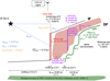 |
Fig. 1 Schematic sketch of the anatomy of the Bar. The dimensions perpendicular to the bar are not to scale but are given at the bottom of the sketch. We also note that foreground material is not depicted. This includes a layer of ionised gas (O’Dell et al. 2020) and the Veil (e.g. Rubin et al. 2011; Boersma et al. 2012; van der Werf et al. 2013; Pabst et al. 2019, 2020). Figure taken from Peeters et al. (2024). |
3 Methodology
3.1 The data
We use the 0.97–28.3 μm spectroscopic observations of the Bar taken with JWST as part of the PDRs4All Early Release Science (ERS) program (ID 12881 ; Berné et al. 2022; Peeters et al. 2024; Chown et al. 2024; Van De Putte et al. 2024). The NIRSpec mosaic is a 9 × 1 mosaic taken with the integral field unit (IFU) mode at high spectral resolution (R ≈ 2700) from 0.9 to 5.27 μm and centred on α = 05:35:20.4749 and δ = −05:25:10.45 with a position angle of 43.74° (Böker et al. 2022). The MIRI observations were taken with the medium-resolution spectroscopy (MRS) observing mode to produce a 9 × 1 pointing mosaic with a spectral resolution R ranging from ~ 1700 to ~ 3700. The MIRI MRS mosaic is positioned to overlap with that of the PDRs4All JWST NIRSpec IFU observations (Peeters et al. 2024). The field of view (FOV) for both mosaics is shown in Fig. 2.
The NIRSpec data were taken from Peeters et al. (2024). The MRS data were re-reduced using version 1.11.1 of the JWST pipeline2, and JWST Calibration Reference Data System3 (CRDS) context jwst_1097.pmap. We refer the reader to Peeters et al. (2024), Chown et al. (2024), and Van De Putte et al. (2024), for a detailed description of the data reduction, calibration and mosaic stitching techniques.
3.2 Data pre-processing
As we aimed to investigate PAH evolution, we isolated the PAH emission features we knew to be associated with PAHs, from our data. We subtracted the continuum emission component and removed spectral lines from each spectrum in the dataset. We used the same line list for removal of spectral lines not attributed to PAHs as was used in Chown et al. (2024), and therefore refer the reader to Peeters et al. (2024) and Van De Putte et al. (2024) for these complete inventories corresponding to the NIRSpec and MIRI MRS datasets, respectively. The continuum components of the spectra from both the NIRSpec and MIRI MRS datasets were the same as those used in Peeters et al. (2024) and Chown et al. (2024), hence we refer readers to Peeters et al. (2024) and Chown et al. (2024) for a detailed description of how the continuum components were derived for both datasets. For the 7.7 μm complex, we used an alternative continuum (a linear continuum instead of a spline continuum) to improve the continuum estimate in the H II region. Edge pixels in both NIRSpec and MIRI datasets often have unreliable data, so we removed these. We also masked out all pixels coinciding with proplyds 203–504 and 203–506 (see Fig. 2) to focus our analysis on the PAH emission at the various depths in the Orion Bar PDR. We made use of the MIRI MRS data shortwards of 13.2 μm and the NIRSpec data between 3.2 and 3.6 μm.
The intensity of the AIB emission varies considerably with distance from the Trapezium cluster (Habart et al. 2024; Peeters et al. 2024; Chown et al. 2024). We found that clustering results without normalisation by total integrated intensity trace solely the variations in the strength of observed AIB emission. To prevent this effect from dominating the cluster assignment (see Sect. 3.3 for a description of cluster assignment), we therefore normalised all continuum-subtracted spectra, cleared of lines, by their total integrated intensity (over the wavelength range considered) prior to clustering. We refer to these final spectra as cleaned, standardised spectra.
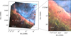 |
Fig. 2 PDRs4All FOVs for both NIRSpec IFU and MIRI MRS datasets are illustrated with the solid and dashed white lines, respectively. The FOVs are overlaid on a composite NIRCam image of the Bar constructed from PDRs4All imaging data (Habart et al. 2024), where red, green, and blue are encoded as F335M (3.3 μm aromatic infrared band emission), F470N-F444W (H2 emission), and F187N (Paschen α emission), respectively. The location of the ionising source, θ1 Ori C, is shown with the white circle in the top right corner of the left panel. The two proplyds, 203–504 and 203–506, are outlined with black circles. Figure adapted from Chown et al. (2024). |
3.3 The clustering algorithm
We employed a bisecting k-means clustering algorithm for this study. We used the open-source Python implementation of the algorithm in the Scikit-Learn library (Pedregosa et al. 2011). This clustering scheme is hierarchical in nature as it combines the strategies of divisive and k-means clustering algorithms to perform cluster assignment. In this context, clusters were interpreted as groups of pixels in a given dataset whose spectra share similar properties. Going forwards, this algorithm may be referred to as ‘the clustering algorithm’.
Bisecting k-means clustering applies a divisive hierarchical clustering scheme (described in detail in Savaresi & Boley 2001; Steinbach et al. 2000; Wang et al. 1998; Zhao et al. 2005) to the cleaned, standardised spectra. Each spectrum in the dataset is assigned a label which designates it as a member of a given cluster. The labelling process is done in a top-down approach which begins by treating the entire sample of spectra as a single cluster before iteratively splitting the clusters further. In each iteration of splitting, the cluster which has the highest variance between members is split into two (‘bisecting’). The splitting of a given cluster into two is done via k-means (e.g. Forgy 1965) clustering, which involves an assignment of cluster members such that the total Euclidean distance between all points and the cluster cen-troid (the data point at the centre of a cluster) are minimised. For this specific use case, distance between two spectra can be interpreted as Euclidean distance between two n-dimensional vectors where each spectrum is a vector, each wavelength position an nth dimension and the intensity there the magnitude of that ‘vector’ component. K-means clustering is also described in detail in Boersma et al. (2014). This process is repeated until either each observation is the only member of each cluster or a preset number of clusters, specified by the user, has been reached. The optimal number of clusters for a given dataset can be determined using a number of analytic methodologies, though whether the optimal number of clusters for a given dataset has been found is outside the scope of this study.
As we do not set out to characterise or classify the PAH emission profiles in the Bar, we employed heuristic methods, such as consulting distortion curves and silhouette scores, strictly to support our analyses. We consulted these metrics to know the quality of our clustering applications only as it supported our understanding of the variation in the local PAH population which we probed.
In order to quantify the quality of cluster assignments throughout our experiments, we fitted our clustering algorithm for a range of total clusters and examine the relationship between the distortion within clusters as a function of the number of clusters. Distortion was calculated as the average sum of squared Euclidean distances between each cluster member and corresponding centroid. The inflection point on this curve (known as the ‘elbow point’) was used to identify the optimal number of clusters detected by the clustering algorithm within the dataset.
We also used a silhouette score (S) to quantify the quality of our clustering. The silhouette score is a value ranging from 0 to 1 that quantifies the goodness of cluster assignment and is given by Eq. (1), where a is the average distance between each point within a cluster and b is the average distance between all clusters:
 (1)
(1)
The silhouette score for a set of clusters close to 0 indicates the clusters are indifferent from one another. At the same time, a score close to 1 indicates that clusters are well-distinguished from one another.
Bisecting k-means is a popular algorithm for many unsupervised learning applications such as document retrieval, pattern recognition and image analysis due to its use of hierarchical binary taxonomy (Zhao et al. 2005; Steinbach et al. 2000). It is also ideal for this science application for multiple reasons. Its hierarchical nature enables us to probe increasingly specific groups of spectra based on both large-scale and more subtle variability. Bisecting k-means also offers improvements over basic k-means clustering in both computational power and the ability to recognize irregularly shaped (non-circular) clusters, especially in cases where the number of clusters is much smaller than the sample size (e.g. Zhao et al. 2005; Steinbach et al. 2000; Bangoria Bhoomi 2014; Ristoski et al. 2015). It is important to note, however, that bisecting k-means does not resolve a fundamental shortcoming of the k-means clustering algorithm, that is, the general convergence on a solution regardless of the dataset (e.g. Selim & Ismail 1984; Banerjee et al. 2015; Di & Gou 2018).
In order to focus cluster assignments on changes in spectral profiles of specific PAH features or regions, we only applied the clustering algorithm to selected wavelength ranges: 3.2–3.6, 5.95–6.6, 7.25–8.95, and 10.9–11.63 μm to cover the main vibrational emission bands at 3.3, 6.2, 7.7, and 11.2 μm, respectively. For each of these experiments pertaining to a single PAH emission band (the 3.3, 6.2, 7.7, and 11.2 μm wavelength regions), a single round of clustering was applied to the input dataset. In the case of the experiment using all the MIRI MRS data shortwards of 13.2 μm, we applied an initial round of clustering to the data with a total of three clusters specified. Three clusters were chosen for this initial round of clustering to capture the H II region, the atomic PDR, and the molecular PDR zones within the MIRI MRS footprint with the intention of focusing subsequent rounds of clustering on the atomic PDR zone. We isolated pixels identified by the clustering algorithm that belonged to the atomic PDR where the PAH emission dominates. We examined the resulting clusters and identified the cluster which coincided spatially most closely with the atomic PDR. We then masked out all pixels which did not belong to this cluster, and applied a secondary round of clustering to this subset of pixels only. We refer to this specific experiment as ‘atomic PDR-focused’ clustering.
For each experiment, once clustering had been applied, the global properties of the spectra belonging to each cluster were analysed by constructing the PAH emission profiles that belong to each cluster. This was done by averaging the intensity at each wavelength position across all cleaned, standardised spectra assigned to a given cluster. In the same way, the standard deviation at each wavelength position was calculated for all cleaned, standardised spectra belonging to the same cluster as a measure of the dispersion within the cluster spectra. Differences between these spectral profiles were then directly compared. We also examined the spatial locations of the pixels belonging to each cluster with respect to physical structures in the Bar such as the IF, and each of the three dissociation fronts.
4 Results
We used clustering as a tool to probe the variation of observed PAH emission in both spatial and spectral dimensions. We emphasise that we did not set out to use the clustering algorithm to classify PAH emission into any discrete number of classes. Instead, we studied this variability to further our understanding of the (photochemical) evolution of the underlying PAH population. At the same time, we tested the abilities of employing such an unsupervised machine learning technique for spectral analysis of PAH emission. We did so by examining the clustering results (Sect. 4) while considering those revealed by traditional spectral analysis methods (Sect. 5).
We report the results for each of the 3.3, 11.2, 6.2 and 7–9 μm region cluster experiments, using a total of four clusters each. For clustering applied with four clusters, the average silhouette scores vary between 0.30 and 0.52 for the above wavelength regions. We found the elbow of the distortion curves for each wavelength range to occur at four clusters (except that of the 7–9 μm region which occurs at five clusters) and the corresponding silhouette scores to be acceptable for the purposes of our analysis. Therefore, we compare the results from each experiment with four clusters and give give the results from clustering with higher numbers of clusters in Appendix B. We also report the results from the atomic PDR-focused clustering experiment for the entire MIRI MRS wavelength range shortwards of 13.2 μm. For each wavelength range experiment, we show the elbow plots in Appendix A and the silhouette scores and elbow points for each in Table A.1.
4.1 The 3.2–3.6region
Many PAH emission bands arise in the 3.2–3.6 μm region, the strongest of which being the 3.29 μm band. Weaker bands arising from PAHs include the 3.25 and 3.33 μm components. We note that the 3.25 and 3.33 μm bands are not as clearly detected in the averaged spectra shown in Fig. 3 as the others (Peeters et al. 2024). The 3.40 μm band is composed of three sub-components centred at 3.395, 3.403, and 3.424 μm (Peeters et al. 2024) and sit on top of a broad plateau emission component in this region (Geballe et al. 1989; Sloan et al. 1997). Unlike the aromatic components which make up the 3.3 μm band, these components arise from aliphatic side groups on PAHs (Joblin et al. 1996; Maltseva et al. 2018; Bernstein et al. 1996; Pla et al. 2020; Buragohain et al. 2020).
The 3.29 μm feature dominates the emission profile in this wavelength region, the 3.4 μm band being weaker. The 3.29 and 3.4 μm bands are the strongest features in the averaged profiles for each cluster. As such, these features largely affect the cluster assignment as seen in the average spectral profiles for each cluster (Fig. 3). Indeed, the cluster profiles clearly trace variations in the 3.4/3.3 peak intensity ratio. In addition, the cluster profiles probe the relative intensity in roughly the 3.33−3.6 μm interval with respect to the 3.29 μm PAH intensity and show subtle variation in the strength of the blue wing of the 3.29 μm band. These variations are linked with each other: enhanced 3.4/3.29 peak intensity ratio corresponds to enhanced overall 3.33–3.6 μm emission with respect to the 3.29 μm PAH intensity and enhanced width of the 3.29 μm profile.
Indeed, the clustering assignment is determined by the emission in the 3.4–3.6 μm wavelength interval. We re-applied the clustering to only the 3.29 μm feature by selecting only the emission in the 3.2–3.36 μm wavelength interval. We found no significant difference between the profiles of the 3.29 μm feature from this round of clustering and the results from clustering on the entire 3.2–3.6 μm range. The cluster zone map from this round of clustering can be found in Fig. B.6. The H II region remains in its own cluster, however a portion of the molecular PDR behind DF 1 now joins the cluster which covers the atomic PDR. The slight broadening of the 3.29 μm feature with increasing distance from the IF as well as the variation in the strength of the blue wing are also observed by Chown et al. (2024) and Peeters et al. (2024).
The spatial zones within the PDR to which each cluster profile corresponds are shown in Fig. 3. The four clusters form very regions in the NIRSpec FOV that are parallel to the IF and thus to the stratification within PDRs. Specifically, the largest region encompasses the atomic PDR and represents cluster 1. This cluster exhibits the smallest 3.4/3.29 peak intensity ratio, the smallest (3.33–3.6)/3.29 emission, and the smallest full width at half maximum (FWHM) of the 3.29 μm PAH. Subsequently, cluster 2 exhibits a slightly enhanced 3.4/3.29 peak intensity ratio with respect to cluster 4. Cluster 2 encompasses the pixels in the H II region, along DF 1, and the region between DF 1 and DF 2. Compared to cluster 2, cluster 3 exhibits again a slightly enhanced 3.4/3.29 peak intensity ratio and originates from DF 2, most of the region between DF 2 and DF 3, and the region beyond DF 3. Finally, cluster 4, with the largest 3.4/3.29 peak intensity ratio, traces DF 3 as well as a small region just behind DF 2.
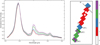 |
Fig. 3 Average spectral profile (left) and spatial footprint (right) for all clusters determined in the 3.2–3.6 μm region. Each cluster is labelled with an integer numbered 1 through 4 (in an arbitrary manner). Left panel: The shaded regions around each profile illustrate one standard deviation from the mean profile intensity at a given wavelength value. Each spectrum is normalised to its peak 3.3 μm intensity for visualisation purposes. Right panel: The spatial footprint of the NIRSpec FOV colour-coded by cluster assignment. Any masked pixels or those that have been otherwise masked out are labelled with 0. The black, dashed lines indicate the locations of the ionisation front (IF) and the three dissociation fronts (DF 1, DF 2 and DF 3) as defined in Peeters et al. (2024) using nomenclature established in Habart et al. (2024). |
4.2 The 5.95–6.6μm region
The 6.2 μm band dominates PAH emission in the 5.95–6.6 μm wavelength region, peaking at 6.212 μm Distinct weaker features also present themselves at 6.024 and 6.395 μm (Chown et al. 2024), but are not strongly pronounced in the profiles of the mean cluster spectra presented in Fig. 4.
The 6.2 μm band very clearly governs the cluster assignment within this wavelength interval as it is the most prominent feature here. We do not observe any variation in the location of the peak intensity for the 6.2 μm band between clusters, though variation in the width of this profile is present. Notably, the red wing of the 6.2 μm band varies slightly more than what is observed for the blue wing. However, variation in the contribution from the 6.024 μm component is observed across clusters. The 6.395 μm component has a very subtle contribution to the 6.2 μm profile which is present only in two of the mean cluster profiles. Once again, these spectral variations correlate with one another. As profiles decrease in width, the 6.024/6.2 intensity ratio also decreases but the prominence of the 6.395 μm feature increases.
We now consider each cluster in order of decreasing FWHM of the 6.2 μm profile. First, cluster 4 has the widest profile with a barely noticeable 6.395 μm component and highest 6.024/6.2 intensity ratio, and is found in DF 3 and a filament behind DF 2. Next, cluster 3 arises in part of the H II region, in DF 2, in most of the region bounded by DF 2 and DF 3, and beyond DF 3. Subsequently, cluster 2 which exhibits a noticeable 6.395 μm component traces the IF and a zone which extends from a hard boundary just in front of DF 2, to a softer, more blended boundary with cluster 1 in front of DF 1. A few pixels at the farthest edge of the FOV from the ionising source behind DF 3 as well as in the H II region also belong to cluster 2. Lastly, cluster 1 has the narrowest 6.2 μm band profile and most obvious presence of the 6.395 μm feature. Cluster 1 covers most of the atomic PDR. The boundaries of the clusters assigned to this wavelength region are mostly parallel to the IF. However, more gradient-like transitions between zones are observed (see the transition between clusters 2 and 1 or between clusters 2 and 3 in the H II region) for this wavelength region which are not observed for the 3.2–3.6 or 10.9–11.63 μm regions.
The pixelation of the boundaries between the clusters from the 6.2 μm wavelength band can be attributed to the fact that the changes probed by the clustering algorithm are (almost) solely the FWHM of the main 6.2 μm band and the variation in the (slight) broadening of this feature takes place very gradually. The pixelation may also be attributed to the nature of bisecting k-means clustering. The clustering algorithm operates under the assumption that all clusters are circular in shape, therefore those variations which deviate from this geometry will not result in well-defined cluster boundaries. If the variation between cluster zones is, in reality, not linearly separable, then the clustering algorithm in general will struggle to establish well-defined boundaries.
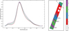 |
Fig. 4 Average spectral profile (left) and spatial footprint (right) for all clusters determined in the 5.95–6.6 μm region. Each cluster is labelled with an integer numbered 1 through 4 (in an arbitrary manner). Left panel: The shaded regions around each profile illustrate one standard deviation from the mean profile intensity at a given wavelength value. Each spectrum is normalised to its peak 6.2 μm intensity for visualisation purposes. Right panel: The spatial footprint of the MIRI MRS FOV is colour-coded by cluster assignment. Any masked pixels or those that have been otherwise masked out are labelled with a 0. The black, dashed lines indicate the locations of the IF, DF 1, DF 2 and DF 3. |
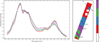 |
Fig. 5 Average spectral profile (left) and spatial footprint (right) for all clusters determined in the 7.25–8.95 μm region. Each cluster is labelled with an integer numbered 1 through 4 (in an arbitrary manner). Left panel: the shaded regions around each profile illustrate one standard deviation from the mean profile intensity at a given wavelength value. Each spectrum is normalised to its peak 7.7 μm intensity for visualisation purposes. Right panel: the spatial footprint of the MIRI MRS FOV is colour-coded by cluster assignment. Any masked pixels or those that have been otherwise masked out are labelled with a 0. The black, dashed lines indicate the locations of the IF, DF 1, DF 2 and DF 3. |
4.3 The 7.25–8.95μm region
There are multiple components to the 7.25–8.95 μm PAH emission (Bregman et al. 1989; Peeters et al. 2002; Cohen et al. 1989), the most prominent of which is the 7.7 μm complex, followed by the 8.6 μm band. The 7.626 μm feature forms the main component of the 7.7 μm complex, accompanied by other strong bands at 7.8 and 7.85 Weak features at 7.43, 8.223 and 8.330 μm are also present, though subtle (Chown et al. 2024).
These features are all observed in the mean spectral profiles for each of the clusters calculated in this wavelength region (Fig. 5). We observe four cluster profiles which vary most noticeably in the width of the 7.7 μm profile and the 8.6/7.7 intensity ratio, as well as in the relative strength of the weaker 7.43 and 7.626 μm components. As the width of the 7.7 μm component decreases, the strength of the 8.6/7.7 intensity ratio increases. The presence of the 7.43 μm component also varies between clusters, though independently from the width of the 7.7 μm complex and the 7.8/7.626 intensity ratio.
The spatial zones of each of these clusters are well-defined (Fig. 5). Cluster 4, which exhibits the widest 7.7 μm profile, covers a large portion of the molecular PDR behind DF 2. This cluster zone is bounded by DF 2 and DF 3, with some pixels belonging to cluster 3 between these bounds. Cluster 4 exhibits the second weakest 8.6/7.7 band intensity ratio and the strongest 7.8/7.626 and 7.85/7.626 band intensity ratios. Cluster 4 also presents the most prominent 7.43/7.626 bump.
Cluster 3 shows a 7.7 μm profile slightly narrower than that of cluster 4 and the weakest 8.6/7.7 and 8.33/7.7 intensity ratios. Cluster 3 is located beyond DF 3 and in two smaller, irregularly shaped regions just in front of DF 3.
The 8.223 μm component of cluster 3 coincides with that of cluster 2. Cluster 2 occupies most of the pixels in the molecular PDR behind DF 1 and in front of DF 2, as well as extends into the atomic PDR. The profile of cluster 2 has a more narrow 7.7 μm complex profile than that of cluster 3 but with an overlapping 8.223 μm component. The 8.330/7.7 and 8.6/7.7 ratios, however, are distinctly enhanced.
Cluster 1 coincides largely with the atomic PDR, with some pixels extending into the H II region as well. The profile of cluster 1 shows the most narrow 7.7 μm profile and highest 8.6/7.7 intensity ratio. Cluster 1 also shows the weakest 8.223/7.7 and second weakest 8.330/7.7 μm intensity ratios.
4.4 The 10.9–11.63 μm region
The 10.9–11.63 μm region is dominated by the 11.2 μm emission band, with weaker bands at 10.95 and 11.005 μm (Chown et al. 2024). The 11.2 μm band is known to exhibit two components at 11.207 and 11.25 μm (Chown et al. 2024).
The 11.2 μm band clearly dominates the PAH emission in the 10.9–11.63 μm region, as such it plays a key role in cluster assignment here. This is observed in the significant 11.2 μm profile variations between cluster spectra as shown in Fig. 6, specifically in the peak positions of the two components and the strength of the red wing for this prominent band. Additionally, more subtle variations in the 11.0/11.2 intensity are observed between the averaged spectral profiles. Profiles for the 11.2 μm band which have a more prominent peak component at 11.207 μm show the weakest red wing and strongest 11.0/11.2 intensity. As peak positions shift to the 11.25 μm component, the 11.0/11.2 intensity decreases, and the 11.2 μm red wing component widens.
Spatial correspondence between zones in the PDR and pixels from cluster assignment are illustrated in Fig. 6. As was the case for the 3.2–3.6 μm region, these cluster zones also exhibit well-defined boundaries roughly parallel to the IF, which correspond to the known physical stratification in PDRs. Cluster 1 arises from the most prominent region and covers most of the atomic PDR, stopping slightly short of DF 1. This cluster exhibits an 11.2 μm profile dominated by the 11.207 μm peak, with the smallest contribution from the 11.25 μm component and weakest red wing. Cluster 1 also corresponds to the strongest 11.0/11.2 band intensity ratio. Cluster 2 traces the IF, part of the H II region along the edge of the FOV closest to the ionising source, and the region surrounding DF 1, stopping just short of DF 2. The profile for cluster 2 also shows a strong 11.2 μm component peaking at 11.207 μm with a slightly stronger red wing than that of cluster 1. Accordingly, this profile has the second strongest 11.0/11.2 band intensity ratio. The 11.0/11.2 intensity ratio of cluster 2 is similar to that of cluster 3, however the 11.2 μm profile appears doubly peaked, with the strongest component at 11.207 μm, though considerable strength in the second 11.25 μm component. Cluster 3 is found in part of the H II region (bounded by those in cluster 2 on both sides, parallel to the IF), in a stripe just in front of DF 2, past DF 3 in a region along the farthest edge of the footprint from the ionising source, and in two small circular regions just in front of DF 3. Finally, cluster 4 is found in the region bounded by DF 2 and extends to the rear of DF 3. This profile has the strongest 11.2 μm component peaking at 11.25 μm the widest red wing, and the weakest 11.0/11.2 intensity ratio.
4.5 Atomic PDR, 4.9–13.2μm region
We use the entire wavelength range from the MIRI MRS dataset shortwards of 13.2 μm in this atomic PDR-focused experiment. We report results from the initial round of clustering on the entire MIRI MRS footprint using three clusters, and using four clusters on the portion of the footprint found to coincide with the atomic PDR from the initial cluster assignment. We also generate increasingly granular stratification within this region using increasingly higher numbers of clusters during the secondary clustering application. We report these findings in Appendix B.
The initial round of clustering yielded three, well-defined zones (Fig. 7). The H II region was assigned to cluster 3, with a hard boundary coincident with the IF (plus a few pixels in the molecular PDR past DF 3 near the farthest edge of the FOV from the ionising source). The atomic PDR and a small portion of the first section of the molecular PDR just behind DF 1 belong to cluster 1. The remaining pixels past the midpoint between DF 1 and DF 2, extending to the far edge of the FOV, are assigned to cluster 2.
We apply a subsequent clustering round to those pixels belonging to cluster 1, exclusively. The cluster zones thus generated are shown in the right-hand panel of Fig. 7. This clustering application returns very well defined clusters with boundaries parallel to the IF, that is, it picks out increasingly granular variations in the local physical conditions. Starting closest to the IF, cluster 2 is bounded by the IF and a stripe of pixels in front of proplyd 203–504. This boundary marks the beginning of cluster 4, covering three main stripes of pixels in the atomic PDR, between which are the pixels belonging to cluster 3. Finally, cluster 1 is centred on DF 1, extending just in front of DF 1 into the deepest layers of the atomic PDR and out into the first layers of the molecular PDR past DF 1 (ending in front of DF 2).
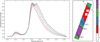 |
Fig. 6 Average spectral profile (left) and spatial footprint (right) for all clusters determined in the 10.9–11.63 μm region. Each cluster is labelled with an integer numbered 1 through 4 (in an arbitrary manner). Left panel: the shaded regions around each profile illustrate one standard deviation from the mean profile intensity at a given wavelength value. Each spectrum is normalised to its peak 11.2 μm intensity for visualisation purposes. Right panel: the spatial footprint of the MIRI MRS FOV is colour-coded by cluster assignment. Any masked pixels or those that have been otherwise masked out are labelled with a 0. The black, dashed lines indicate the locations of the IF, DF 1, DF 2 and DF 3. |
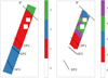 |
Fig. 7 Spatial footprint of the MIRI MRS FOV is colour-coded by cluster assignment calculated on an initial (left) and secondary (right) round of clustering on all spectral features in the MIRI MRS dataset shortwards of 13.2 μm. The secondary round of clustering was applied only to those pixels belonging to cluster 1 in the initial round of clustering that largely coincide with the atomic PDR. Clusters are labelled 1 through 4 (in an arbitrary manner) and masked pixels are labelled 0. The black, dashed lines indicate the locations of the IF, DF 1, DF 2 and DF 3. |
5 Discussion
We begin our discussion by noting that trends in the spectral characteristics of the PAH emission captured by the clustering algorithm align very closely with those reported by Peeters et al. (2024) and Chown et al. (2024). In both studies, template spectra were selected from five regions probing the key zones in the Bar. In addition, Peeters et al. (2024) reported on the 3.2–3.7 μm PAH emission variability across the NIRSpec mosaic. Chown et al. (2024) established that spectral variations in this region are linked to spatially distinct regions (as opposed to a slowly changing behaviour). Our study serves to expand on these results by applying unsupervised machine learning to more spatial data (Chown et al. 2024) and spectral data (Peeters et al. 2024). We report an elaborate map of the variation in the PAH emission throughout the Bar based on the study of the entire NIRSpec and MIRI MRS FOVs. The consistency between our results and those of these authors therefore highlights the excellent range in spectral variability captured by the five template spectra in these previous studies.
5.1 Connecting the clustering results on different PAH emission regions
We applied the clustering algorithm to several individual, disjoint wavelength regions which exhibit strong PAH emission bands. While the spatial locations of each of the cluster zones for each wavelength region do not necessarily correspond one-to-one, we find a relationship between the changes in the mean spectral profiles for each of the cluster assignments. That is to say, the variations observed in the PAH bands, traced by the clustering results, are connected to one another.
In general, those regions which exhibit a strong 3.4/3.3 intensity ratio will also demonstrate broader 6.2 and 7.7 μm bands, a weaker 8.6/7.7 band intensity ratio, and likely a so-called class B profile for the 11.2 μm feature. The same trend follows for many of the weaker PAH bands as well. For example, these same cluster profiles will also show stronger 3.424 μm component and 3.52 μm components in the 3.2–3.7 μm complex, and a weaker 11.005 μm component in the 11 μm region. In contrast, those clusters which select spectra for their weaker 3.4/3.3 intensity ratio will correspond to those profiles which also show more narrow 6.2 and 7.7 μm profiles, stronger 8.6/7.7 band intensity ratios, and will have a class A 11.2 μm profile peaking closer to 11.207 μm. At the same time, the 3.424 μm and 3.52 μm components will weaken and the 11.005 μm component will strengthen.
It is also interesting to note that the clustering results can be used, in some cases, to predict the cluster assignments in other wavelength ranges. Indeed, we find that clustering results calculated on the 11.2 μm wavelength region recover strikingly similar clustering results for the 6.2 μm region (see Fig. 8). The only major difference between the mean cluster spectra, noticeable by eye, concerns the relative sizes of the 1σ deviations of the cluster profiles. The variances in the 6.2 μm profiles calculated using the 11.2 μm cluster assignments are slightly larger than those that were calculated using the 6.2 μm profile itself. This is to be expected, given that the clusters were not assigned based on this information. Overall, the cluster zones themselves also overlap with one-another quite well. The clusters which coincide with the major zones in the PDR such as the atomic PDR, molecular PDR, IF, and H II region all agree for the majority of their pixels. Deviations between the zones are most noticeable in the boundaries of the clusters themselves, as well as especially between the zones which lie between DF 2 and DF 3. The cluster zones originating from the 11.2 μm region largely assign the region of pixels bounded by DF 2 and DF 3 to a single cluster, except for a few smaller groups of pixels. In the case of the clusters assigned based on the 6.2 μm band, this same cluster largely just traces DF 3 and the filamentary structure of pixels just behind DF 2. This result suggests an intrinsic connection between the 11.2 and 6.2 μm bands. The carriers of the 11.2 and 6.2 μm bands are known to be largely neutral and cationic, respectively (e.g. Allamandola et al. 1999). Conditions at the origin of the variation in the 11.2 μm band are thus also at the origin of the variations seen in the 6.2 μm band. We discuss possible carriers in relation to these variations in Sect. 5.4.
Such a very strong connection between clustering results is not found for other combinations of the other wavelength regions explored in this study. We illustrate comparisons between the results generated from clustering on the 7.25–8.95 and 3.2–3.6 μm regions with those derived from the 10.9–11.63 μm region in Appendix C. As for the 6.2 μm results, the average spectral profiles in the 7.25–8.95 and 3.2–3.6 μm regions derived from the clustering results of the 10.9–11.63 μm region (see Figs. C.1 and C.2, respectively) are less well defined (i.e. have enhanced variance). Moreover, they also probe a slightly smaller range in spectral variability. Nevertheless, these results showcase the power of this clustering algorithm as a predictive tool in spectral analysis of PAHs. Should, for example, only a limited wavelength range be available for study, the variations in profiles outside of this wavelength range can be extrapolated, though this has yet to be confirmed by other studies for other PDRs. This could be done using results from a clustering application to the data available and knowledge of the connection between the bands observed and those that are connected to the observed bands, but not observed themselves.
Our application of clustering on the 11.2 μm wavelength region reveals the detailed, gradual transition between the class A and B profiles for the 11.2 μm band. Indeed, our cluster zones, coupled with the corresponding mean spectral profiles, act as a detailed map for this transition. Upon inspection of clustering results for increasingly higher numbers of clusters than four, we trace this transition in greater detail.
In Fig. B.4, for seven clusters (the highest number of clusters explored in this study), we see the transition between class A11.2 and class B11.2 profiles given by the cluster zones in great detail. The transition from class A to class B can be described spec-troscopically by a slightly decreasing and redshifting 11.207 μm component combined with an increasing and slightly redshifting 11.25 μm component. Combined, this results in a less steep blue wing and enhanced red wing for the class B profiles with respect to class A profiles.
Those profiles which correspond to class A11.2 originate in the atomic PDR, and transition to class B11.2 profiles with distance from the ionising source. The purple, green, red and blue clusters show the strongest class A11.2 profiles, in decreasing order. The green zone occupies a group of pixels in one of the outermost layers of the atomic PDR, slightly in front of DF 1, as well as a thin stripe of pixels just behind the IF and through the middle of the atomic PDR zone. The red zone lies just in front of DF 1 and as well consists of a small band of pixels just behind the IF. The blue profile originates largely between DF 1 and DF 2 but also with some pixels in the H II region. We are also able to observe, for this number of clusters, more nuance to the intermediate class A(B)11.2 profiles. These orange and brown profiles belong largely to the region after the mid-point between DF 1 and DF 2, excluding DF 3, with some clusters in the H II region as well. The strongest class B11.2 profile, belonging to the yellow cluster, solely traces DF 3.
Our clustering results suggest that the carriers of the class B11.2 profile originate largely in DF 3. The carriers of the class A11.2 profiles are located throughout the Bar, primarily in the atomic PDR. However, the cluster zones indicate a transition to the intermediate class profile when you travel both away from and in front of the IF (we note that in the latter case the PAH emission arises from the background PDR). When moving towards the molecular PDR, we also see the broadening of most PAH emission profiles and an intensifying 3.4/3.3 band ratio. The carriers of the class B11.2 profiles thus originate in the much colder conditions of the molecular PDR, especially within DF 3 itself. The regions in the cluster zone map given in Fig. B.4 (along DF 3 and a filament just behind DF 2, seen in numbers of clusters greater than 4) for 11.2 μm which align with the most pronounced class B profile are also picked out for the 3.3 and 6.2 μm wavelength regions. These structures are not as well defined in the case of the 7–9 μm region where they begin to appear with six clusters (see Fig. B.3).
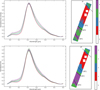 |
Fig. 8 Average spectral profiles (left) for the 6.2 μm band obtained from clustering assignment based on the 5.95–6.6 μm region and the corresponding cluster zones (right) are given in the top two frames. The average spectral profiles (left) for the 6.2 μm band obtained from clustering assignment based on the 10.9–11.63 μm region and the corresponding cluster zones (right) are given in the bottom two frames. Left panels: the shaded regions around each profile illustrate one standard deviation from the mean profile intensity at a given wavelength value. Each spectrum is normalised to the peak 6.2 μm intensity for visualisation purposes. Right panels: the spatial footprint of the MIRI MRS FOV colour-coded by cluster assignment. Any masked pixels or those that have been otherwise masked out are labelled as 0. The black, dashed lines illustrate the locations of the ionisation front (IF) and the three dissociation fronts (DF 1, DF 2 and DF 3) as defined in Peeters et al. (2024) using nomenclature established in Habart et al. (2024). |
5.2 Clustering probes the changing physical conditions
We emphasise again that we removed the effects of total intensity from each of the PAH emission regions prior to any of our clustering experiments (by normalising the input spectra). Nevertheless, the clusters pick up spectral variation corresponding to different regions in the PDR structure consistently for each of the wavelength bands used to generate the clusters as illustrated by the spatial morphology of various cluster zones (Figs. 3 to 6).
We find the atomic PDR, for example, to be largely uniform for the clusters calculated on the main PAH bands (the 3.3, 6.2, 7–9 and 11.2 μm wavelength regions). In the case of the 3.3 μm region, the atomic PDR is covered entirely by a single cluster, even though seven clusters (see Fig. B.1) while for the other wavelengths just two clusters are found for the atomic PDR (with one of them covering most of this zone). Similarly, our clustering results cover the H II region quite consistently between experiments. In all cases, the H II region is mostly covered by a single cluster, with some variance in the shape of this cluster zone between those from the 3.3 and 7–9 μm region results and those from the 6.2 and 11.2 μm regions. In contrast to the other wavelength regions, the 7–9 μm results assign the H II region and atomic PDR zones to the same cluster. This is attributed to the complex interaction of an increased number of spectral features present in this extended wavelength regime and their varied dependencies on the local radiation field. The outer zone of the molecular PDR is identified in a similar fashion for all clustering results based on the 3.3, 6.2 and 7–9 μm wavelength regions. This cluster zone, in each experiment, is well bounded by DF 1 along the edge closest to the IF, and bounded by pixels varying in position from along DF 2 in the case of the 3.3 μm band results, slightly in front of DF 2 in the case of the 6.2 μm band and 79 μm region results. The clustering results based on the 11.2 μm feature instead group pixels centred on DF 1, cutting into both the atomic PDR and the outer region of the molecular PDR. This cluster zone also corresponds to a stripe of pixels along the IF and at the edge of the MIRI FOV closest to the ionising source. Finally, the deepest zone of the molecular PDR, behind DF 2, shows the most structure in the clustering results of any of the zones. This structure is captured by the clusters corresponding to all four of the major wavelength regions explored and becomes increasingly detailed when greater numbers of clusters are used (see Figs. B.1 to B.4). Most notably, the clustering identifies two filamentary patterns, the first of which coincides with DF 3, the second of which lies just behind of and at a slight angle with DF 2.
Overall, we find the molecular zone is split largely into two distinct clusters. One of which corresponds to the outermost region of the molecular PDR, overlapping DF 1, and the second corresponding to the deeper regions of the molecular PDR, coinciding with DF 2 and DF 3. In the case of the cluster zones derived from the 11.2 μm region, this second cluster zone is quite uniform. In the cases of the cluster zones derived from the 3.3, 6.2, and 7–9 μm regions, however, this zone is seen to be split further between a cluster which traces DF 3 and a filament slightly behind DF 2 (the filament behind DF 2 is not apparent in the zone map for the 7–9 μm region). For all cases, though, we observe that the spectral characteristics of the cluster corresponding to DF 1 behave more like to those arising from clusters covering the atomic PDR and H II region than those arising from the secondary molecular PDR cluster coincident with DF 2 or DF 3 (see Figs. 3 to 6). This observation is consistent with the result reported by Peeters et al. (2024) and Chown et al. (2024) that the spectra originating in DF 1 often behave more like those originating in the atomic PDR and H II region than those originating in DF 2 or DF 3. Habart et al. (2024) and Peeters et al. (2024) reported that DF 1 is likely located at a greater distance from us than are DF 2 and DF 3. Hence, a larger column of the atomic PDR is present in this line of sight (Fig. 1) which may be driving the characteristics of the PAH emission along it (Peeters et al. 2024).
Local physical conditions determine the characteristics of the PAH emission bands we observe. In other words, our clustering results, based on varying spectral characteristics of the PAH emission, trace the physical conditions which give rise to these properties.
5.3 Comparison with previous observations
5.3.1 Relative intensity variation
The clustering highlights several variations in relative intensity ratios. The observed dependence of the 3.4/3.3 ratio with distance from the IF and thus with decreasing intensity of the FUV radiation field is well established and attributed to the lower stability of the 3.4 μm band carrier (e.g. Geballe et al. 1989; Joblin et al. 1996; Sloan et al. 1997; Mori et al. 2014; Pilleri et al. 2015). The clustering extends this behaviour to the 3.46, 3.51, and 3.56 μm bands (relative to the 3.3 μm band). We furthermore observe an increased importance of the 6.0 μm band (relative to the 6.2 μm band) with increasing depth into the PDR. Such a behaviour is consistent with the morphology of both bands in reflection nebulae (Peeters et al. 2017; Knight et al. 2022b). In contrast, the 11.0/11.2 ratio decreases with depth into the PDR due to a decreasing ionisation fraction of the PAH population (e.g. Rosenberg et al. 2011; Peeters et al. 2012; Boersma et al. 2013; Peeters et al. 2017; Knight et al. 2022a,b). Finally, relative intensity variations between the 7.6, 7.8, and 8.6 μm bands are commonly observed. The 7.6/7.8 ratio decreases with decreasing strength of the radiation field (e.g. Boersma et al. 2014; Peeters et al. 2017; Stock & Peeters 2017) and the 8.6/7.7 ratio increases with increasing strength of the radiation field (Peeters et al. 2017; Knight et al. 2021, Knight et al. 2022b).
5.3.2 Profile variation
Using a set of template spectra of the key zones in the Bar, Chown et al. (2024) reported class A profiles for the 3.3, 6.2,7.7, and 8.6 μm bands, consistent with our results. These authors also found the profiles of the 11.2 μm band to belong to class A in the atomic PDR and to class B deep in the molecular PDR (DF 2, DF 3). This paper further extends these results to the entire mosaic. While a spatial evolution of the 11.2 μm band profile with distance to the ionising source had previously been reported for reflection nebulae (Boersma et al. 2013, 2014; Shannon 2016), the PDRs4All observations of the Bar report, for the first time, a class B11.2 profile in the ISM and show the transition between class A11.2 and B11.2 (this paper and Chown et al. 2024). Our clustering results as well as Chown et al. (2024) for the five template spectra also capture a broadening of the 7.7 μm band in the direction away from the ionising source. A broadening of the 7.7 μm profile has previously been observed (e.g. Bregman & Temi 2005; Boersma et al. 2014; Stock & Peeters 2017). To our knowledge, a broadening of the A3.3 or A6.2 has not been previously reported within the ISM.
5.3.3 Basis set of PAH components
A powerful analysis approach of PAH observations is the mathematical decomposition of PAH emission spectra as a linear combinations of elementary spectra using blind signal separation (BSS) methods (e.g. Boissel et al. 2001; Rapacioli et al. 2005b; Berné et al. 2007). The obtained basis set of elementary spectra details spatially different components of the observation, thus each component of the basis set has its unique morphology. Generally, three components have been derived which have been associated with neutral PAHs, cationic PAHs, and evaporating very small grains (eVSGs) or PAH clusters (Berné et al. 2007; Pilleri et al. 2012). The strength of the 7.7/11.2 ratio is strongest in the cationic PAH component spectrum and weakest for the neutral PAH component spectrum. The eVSGs component spectrum is quite distinct and exhibits slightly redshifted bands, significantly broadened 7.7 and 11.2 μm profiles and no 8.6 μm feature (Berné et al. 2007; Foschino et al. 2019). These studies found that the eVSGs and PAH clusters components exist in deeper regions of the PDR, far from the ionising source. Indeed, a transition, driven by photoprocessing, from clusters of PAHs to neutral PAHs and eventually to PAH cations resulting from the increasing strength of the UV radiation field occurs as distance to the ionising source decreases (Cesarsky et al. 2000; Boissel et al. 2001; Rapacioli et al. 2005b; Berné et al. 2007; Pilleri et al. 2012). This is consistent with our clustering results which also trace a layered stratification across the Bar which corresponds to varying spectral characteristics as given in our cluster zone maps. Pilleri et al. (2012) reported a strong negative correlation between the fraction of eVSGs or PAH clusters and the strength of the local UV radiation field for several PDRs. These observations serve as evidence for the existence of a photodestruction process that breaks eVSGs or PAH clusters down into PAH molecules. Evidence for eVSGs as carriers for the class B profiles identified in Peeters et al. (2002) has also been found (Foschino et al. 2019). These studies substantiate evidence for PAH clusters as carriers for ‘component 2’ of the 11.2 μm profile we detect far from the ionising source (see Sect. 5.4).
5.4 Astrophysical implications
5.4.1 The 3.2–3.6 μm region
While the 3.3 μm profile has been attributed to the aromatic C-H stretching mode (e.g. Allamandola et al. 1989; Puget & Léger 1989), various candidates have been put forward for the carrier of the components in the 3.4–3.6 μm region. These include the aliphatic C-H stretching mode in methyl (−CH3) and methylene (−CH2) side groups of PAHs (Allamandola et al. 1989; Joblin et al. 1996; Maltseva et al. 2018; Buragohain et al. 2020; Steglich et al. 2013) and in super-hydrogenated PAHs (Bernstein et al. 1996; Wagner et al. 2000; Sadjadi et al. 2015; Maltseva et al. 2018; Sundararajan et al. 2019; Buragohain et al. 2020; Pla et al. 2020; Yang et al. 2020), overtones of the aromatic C-H stretching mode (Barker et al. 1987), combination bands (Allamandola et al. 1989), and a combination thereof. Additional information on the carrier candidates can be obtained from the scissoring modes of aliphatic C-H at 6.85 and 7.35 μm and out-of-plane C-H bands in the 12–15 μm. However, Chown et al. (2024) reported that the aliphatic bands at 6.85 and 7.35 μm are very weak (and only present in the template spectra of DF 2 and DF 3 in a large extraction aperture). Furthermore, inclusion of bands in the 12–15 μm region to the clustering experiments do not add new information. Several studies reported that the relative importance of the aliphatic bands with respect to the aromatic bands decreases with increasing intensity of the FUV radiation field reflecting that aliphatic bonds are less stable than aromatic ones (Geballe et al. 1989; Joblin et al. 1996; Sloan et al. 1997; Mori et al. 2014; Pilleri et al. 2015; Lai et al. 2020, 2023). The clustering results clearly indicate a concerted behaviour of the bands in the 3.4–3.6 μm region: the 3.4 complex, 3.46, 3.51, and 3.56 μm bands all vary in the same fashion, peaking in DF 3 and the region slightly behind DF 2. This behaviour is confirmed by the morphology of these band intensities individually (Peeters et al. 2024). This concerted behaviour of the 3.4–3.6 μm emission implies that the carriers of each of these components must all be most abundant in DF 3 and either get destroyed or evolve in the same way into carriers of other bands in the other PDR zones. We note that the distinct behaviour of the intensities of the components making up the 3.4 μm complex (3.395, 3.403, and 3.424 μm components), as reported by Peeters et al. (2024), is also picked up by the clustering algorithm. Indeed, the morphological similarity of the 3.395 μm band intensity to the 3.29 μm band intensity instead of the 3.403 μm intensity is recovered in the 3.4 μm band profile of the mean cluster profiles (Fig. 3). We are compelled by the similarity of the spatial variation of the 3.4–3.6 μm emission bands to hypothesise that their carriers originate from the same PAH side group attached to similar-sized PAHs. Their concerted spatial behaviour requires that their carriers have similar sensitivity to photolysis. Different bonds within aliphatic subgroups attached to PAHs have distinct dissociation rates (Joblin et al. 1996; Tielens 2008). Our clustering results therefore point to a single sidegroup that is responsible for the observed emission. Furthermore, the dissociation rate for a given bond within an aliphatic subgroup depends on the size of the PAH to which it is attached (Joblin et al. 1996; Tielens 2008). Combined with the dependence of the PAH excitation on size (Schutte et al. 1993), our results further suggest that this sidegroup is attached to similar-sized PAHs. Further, we eliminate resonances between CC and CH in-plane bending modes from the possible causes of this uniform variation of features in this wavelength region. We do not observe what would be consequential shifts in the peak position of the 3.3 μm feature or blending on the red wing as traced by our clustering results (Mackie 2018; Mackie et al. 2022). Finally, we exclude superhydrogenated PAHs as the carriers of the 3.4 μm band in the Orion Bar based on the fact that superhydrogenated PAHs only reside in very benign environments and cannot be the carriers of the 3.4 μm band in the reflection nebula NGC 7023 (Andrews et al. 2016). Further investigation is required to identify the carriers of the bands in the 3.4–3.6 μm region.
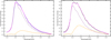 |
Fig. 9 Linear combinations of the class A11.2 profile and a ‘secondary component’ that recover the ‘intermediate’ 11.2 μm profiles of clusters 3 (left) and 2 (right) from the 10.9–11.63 μm wavelength region (see Sect. 5.4 for details). The cluster profile is shown in blue and green in the left and right panel respectively. The dashed purple line represents the scaled class A11.2 profile given by cluster 4, the dashed orange line is the secondary component, and the bright magenta line represents the linear combination of these two components. We note that the small undulations in the red wing of the profiles are residual fringes present due to incomplete fringe removal. |
5.4.2 The 11.2 profile classes
The clustering results for the 11.2 μm band suggest the presence of at least two components, one carrying the 11 .207 component and the other one carrying the 11.25 μm component. The former component dominates the class A11.2 profile while the latter dominate the class B11.2 profile. The transition between both classes can then be interpreted as a changing relative importance of these two components. To investigate this hypothesis, we take the cluster profiles for the 10.9–11.63 μm region, normalised to peak intensity, and decompose the class B11.2 profile from our clustering results (given by cluster 4; Fig. 6) into a linear combination of the class A11.2 profile (given by cluster 1) and the difference between the class B11.2 profile and a secondary component. We determine this secondary component (referred to as component 2) by subtracting the scaled class A11.2 profile (77%) from the class B11.2 profile. We find 0.77 to be the suitable coefficient by which to multiply this secondary component by manual experimentation with the aim to scale the class A11.2 profile to fit entirely inside the B11.2 profile. We can successfully re-create the other normalised cluster profiles using linear combinations of component 2 and the class A11.2 profile (Fig. 9)4. Certainly, the carriers of each of the class A11.2 and B11.2 components are independent.
We propose that PAH clusters or VSGs carry this 11.25 μm component. These PAH clusters (or VSGs) must exist predominantly in DF 3, deep into the molecular PDR, as visualised by the cluster zones in Fig. 6 as well as by the ratio of the surface brightness at 11.25 μm to the surface brightness at 11.207 μm (after continuum subtraction) illustrated in Fig. 10. This intensity ratio map shows the 11.25 μm component peaking over the 11.207 μm component in DF 3. The carriers of the 11.25 μm component must also be independent of the carriers of the 11.207 μm component, as demonstrated in Fig. 9, and thus exist solely in the deeper regions of the PDR, furthest from the IF. This can be attributed to the fact that the binding energy of PAH clusters is low (~50 meV per C atom, e.g. the binding energy for a coronene cluster is ~2.5 eV; Tielens 2021). PAH clusters or VSGs can easily be photolysed due to the increasing FUV radiation field in the direction of the PDR surface at the IF.
Though we do see variation in the other bands studied here which also vary as function of increasing distance from the IF (for example, the intensifying of the 3.4/3.3 band ratio and the broadening of the band profiles), we do not see any other emission band component which appears or disappears in this fashion for any of the other zones in the PDR. Hence, there is no evidence in our results that point to a new contribution in any of the shorter-wavelength bands. The carriers of the 11.25 μm component must then undergo a molecular transition in the photolysis process such that they do not affect the other bands emitting shorter wavelengths. These carriers, the PAH clusters, are molecular predecessors to the carriers of the bands located at shorter wavelengths.
However, it is important to note that we do indeed observe broadening in several shorter wavelength bands in DF 3 compared to those in the atomic PDR (this paper, Peeters et al. 2024; Chown et al. 2024). In addition, while we attribute part of the broadening of the 11.2 μm band to the relative importance of 2 individual components (A11.2 profile and component 2; Fig. 9), component 2 has a broader profile than the A11.2 profile. Spectral broadening is generally attributed to more highly excited species and Peeters et al. (2024) and Chown et al. (2024) concluded that smaller, labile PAH species are present in DF 3 and not in the atomic PDR. The fact that the clustering results calculated on the 11.2 μm wavelength region recover strikingly similar clustering results for the 6.2 μm region (see Fig. 8) then implies that these smaller, labile PAH species and PAH clusters are equally sensitive to photolysis and both are destroyed as the FUV radiation field increases in the direction towards the PDR surface. Moreover, a similar effect on these smaller species can then be expected for the 11.2 μm emission as for the shorter wavelength band profiles in DF 3. This then implies that the width of the blue component in our linear decomposition (A11.2 profile) slightly increases from the atomic PDR towards DF 3 as observed for the shorter wavelength bands. This broadening of the blue component of the 11.2 μm profile due to the smaller-sized PAH population however does not dominate the observed changes in the 11.2 μm profile which is driven by the relative contribution of the PAH clusters. In addition, the larger width of component 2 with respect to that of the blue component then reflects different emission characteristics of PAHs and PAH clusters.
A broader 11.2 μm emission band is also observed in the template spectrum assigned to PAH clusters obtained with BSS (Sect. 5.3.3; Berné et al. 2007; Pilleri et al. 2012; Foschino et al. 2019; Rosenberg et al. 2011). This BSS template spectrum is dominated by a broad emission band peaking near 8.0 μm, has additional emission bands near 6.2 and 3.3 but lacks a well-defined emission band near 3.4 Hence, this template spectrum associated with PAH clusters differs from the emission attributed to PAH clusters in this paper. We note that regions with an enhanced population of PAH clusters exhibit increased emission in the 8.0 μm region. This enhanced emission extends to longer wavelengths with respect to the broad 8.0 μm emission band in the BSS template associated with PAH clusters and we find no evidence in our results that point to a new contribution. Given that the wavelength of the in-plane bending modes of PAHs increases with increasing PAH size (e.g. Bauschlicher et al. 2008; Bauschlicher 2009) and with decreasing PAH edge defects (such as bay regions, Peeters et al. 2017, Ricca et al. 2024), this enhanced emission may arise from smaller PAHs or PAHs with more edge defects. The clustering results indicate that the population in DF 3 consists of smaller, labile PAHs (with respect to those in the atomic PDR) and PAH cluster that are equally sensitive to photolysis. As such, the BSS method may be less sensitive to the distinction of both populations as it relies on spatial variation. However, we note that the BSS method was applied to a mosaic of low spectral resolution data (Berné et al. 2007; Pilleri et al. 2012) as well as integrated medium spectral resolution data (without spatial information; Foschino et al. 2019). Hence, a firm conclusion about this difference awaits the results of the BSS method applied to the same dataset as used here (for the NIR AIBs, see Schroetter 2024). The BSS results also indicated that the contribution of PAH clusters increases with decreasing strength of the FUV radiation field (Pilleri et al. 2012). This is consistent with our findings that the relative contribution of component 2 increases with distance from the IF (Figs. 6, 9, and B.4) suggesting a dependence on the strength of the local FUV radiation field. This then extends the reported dependence of the central wavelength of the 11.2 μm bands in circumstellar environments on the effective temperature of the central star (which is a indication of the strength of the radiation field impinging on the PAH population; Sloan et al. 2007; Keller et al. 2008) to resolved PDRs.
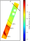 |
Fig. 10 Spatial morphology of the 11.25/11.207 intensity ratio (i.e. the ratio of the surface brightness at 11.25 μηι to the surface brightness at 11.207 μm after continuum subtraction). The 11.25 μm component dominates over the 11.207 μm component in the deeper regions of the PDR, past DF 1, especially in DF 3. |
6 Conclusions
We performed a variability analysis on the PAH emission in the Orion Bar using bisecting k-means clustering, an unsuper-vised machine learning algorithm. We applied this clustering algorithm to spectra from both NIRSpec-IFU and MIRI-MRS onboard JWST for the 3.2–3.6 μm region in the case of the NIRSpec data, and the 5.95–6.6, 7.25–8.95 and 10.9–11.63 μm regions for the MIRI-MRS dataset. These regions were selected as they correspond to major vibrational emission bands of PAHs at 3.3, 6.2, 7.7, and 11.2 μm, respectively. Specifically, we generated mean spectral profiles for each cluster calculated from the PAH emission in each of these wavelength regions, as well as detailed spatial maps associated with each cluster throughout the Bar. This wealth of spatial and spectral data has allowed us to connect variations between bands with one another as well as to derived a nuanced understanding of the variation in the underlying PAH populations across the Bar’s varying physical conditions.
Applying the bisecting k-means clustering algorithm to multiple prominent PAH emission profiles results in well-defined cluster zones that correlate with the spatial stratification of physical conditions within the Bar across the ionised to the molecular, UV-shielded zone. We find that clustering captures subtle differences in profile changes driven by the strength of the local FUV radiation field. In addition, our clustering application on the 10.9–11.63 μm wavelength region reveals the transition between class A and class B 11.2 μm band profiles as defined in van Diedenhoven et al. (2004), consistent with the results of Chown et al. (2024). We also find that the clustering application calculated on the 10.9–11.63 μm region reproduces the cluster assignments for the 5.95–6.6 μm region.
Our clustering results capture a united behaviour in the bands which make up the 3.4–3.6 μm region. They are found to exist most abundantly in the Bar in DF 3, and evolve or are destroyed with increasing FUV radiation in the direction towards the IF. We deduce, from the similarity in the spatial variation in these bands, that they are carried by the same PAH side group attached to similarly sized PAHs. We also reveal that the carriers of the 11.207 and 11.25 μm components of the 11.2 μm profile, which dominate the class A11.2 and B11.2 profiles, respectively, are independent. We have extracted the two components of the 11.2 μm feature which may help in the identification of their carriers. We propose PAH clusters or VSGs to be the carriers of the 11.25 μm component, as they are found to exist solely in the deeper regions of the PDR and their low binding energies dictate their destruction in the direction towards the IF. Finally, we find a dependence on the characteristics of the 11.2 μm profile and the strength of the FUV radiation field.
Our clustering results shed light on the morphology of the physical zones within the Bar in great detail. Clustering on PAH emission, which is coupled to local physical conditions, therefore also identifies clusters of spatial regions which share similar physical conditions. These clusters, coupled with their corresponding spectral information, outline the specific physical conditions for each zone as well as give context for relative differences or similarities between those of the other clusters. Though, at this point in time, the exact physical or chemical processes which control the evolution of the interstellar PAH family (and therefore the observed spectral variations) are unknown. Future observations with JWST and the Atacama Large Millimeter Array (ALMA), for example, may shed light on this. Such observations may, when coupled with PAH spectra and a similar clustering analysis, provide astronomers a tool for pinpointing these varying physical conditions in galaxies far away. Cluster zone maps therefore offer detailed maps which highlight transitions between physical zones limited only by spatial resolution. In this way, a clustering application on PAH emission is a much more powerful tool for identifying variations in physical conditions than what may be the case from studying intensity variations between lines alone.
Overall, we find extraordinary potential for unsupervised machine learning techniques, namely clustering algorithms, as PAH spectral analysis tools. The consistency of our results with those of existing studies which employ traditional spectral analysis methods (e.g. Peeters et al. 2024; Chown et al. 2024) validates the use of such a technique in this space.
Further focused studies on PAH emission in the 3.2–3.6 and 11.2 μm emission regions may uncover greater insight into the carriers of the 3.4–3.6 μm emission and the class B11.2 profiles. Future studies regarding the use of unsupervised machine learning in astrochemistry will lead to an enhanced understanding of the abilities of such algorithms within the context of such spectral analyses. We have only just begun to highlight the potential that such clustering algorithms can have for PAH variability studies.
Acknowledgements
This work is based on observations made with the NASA/ESA/CSA James Webb Space Telescope. The data were obtained from the Mikulski Archive for Space Telescopes at the Space Telescope Science Institute, which is operated by the Association of Universities for Research in Astronomy, Inc., under NASA contract NAS 5-03127 for JWST. These observations are associated with programme #1288. Support for programme #1288 was provided by NASA through a grant from the Space Telescope Science Institute, which is operated by the Association of Universities for Research in Astronomy, Inc., under NASA contract NAS 5-03127. E.P. and J.C. acknowledge support from the University of Western Ontario, the Institute for Earth and Space Exploration, the Canadian Space Agency (CSA, 22JWGO1-16), and the Natural Sciences and Engineering Research Council of Canada. Studies of interstellar PAHs at Leiden Observatory (AT) are supported by a Spinoza premie from the Dutch Science Agency, NWO. C.B. is grateful for an appointment at NASA Ames Research Center through the San José State University Research Foundation (80NSSC22M0107). T.O. acknowledges support from JSPS Bilateral Programme, Grant Number 120219939.
Appendix A Elbow plots
The elbow plots generated for each of the 3.2–3.6, 5.95–6.6, 7.25–8.95, and 10.9–11.63 μm wavelength regions are given in Fig. A.1. The elbow plots generated prior to the initial and secondary rounds of clustering involving in the Atomic-PDR-focused clustering experiments are given in Fig. A.2. We also report the silhouette scores and elbow points for each experiment in Table A.1.
Average silhouette scores and elbow points for each of the clustering experiments are given.
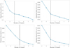 |
Fig. A.1 Distortion scores for clustering applied in the 3.2–3.6, 5.95–6.6, 7.25–8.95, and 10.9–11.63 μm region plotted as a function of the number of clusters used. The inflection point, or ‘elbow’, in the distortion curve is highlighted with the dashed black line. As is shown, four clusters are optimal for each wavelength regime. |
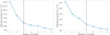 |
Fig. A.2 Distortion scores for clustering on the first (left) and second (right) round of clustering for the 4.9–13.2 μm region in the MIRI MRS dataset as a function of the number of clusters used. The inflection point, or ‘elbow’, in the distortion curve is highlighted with the dashed black line. In the case of the first round of clustering across the entire, cleaned MIRI MRS footprint, four clusters are optimal. In the case of the clustering focused to pixels belonging to the cluster coincident with the atomic PDR, five clusters are optimal. |
Appendix B Further clustering applications
Averaged spectral profiles for clusters calculated on each of the 3.2–3.6, 5.95–6.6,7.25–8.95 and 10.9–11.63 μm wavelength regions were calculated on a number of clusters ranging from three to seven, inclusively. These average cluster profiles along with the corresponding spatial maps for the cluster zones, are given in Figs. B.1, B.2, B.3 and B.4, respectively, and for the 4.9–13.2 um region in Fig. B.5. The mean spectral profile and corresponding cluster zone map for the clustering application on the 3.29 μm feature (from 3.2–3.36 μm are given in Fig. B.6.
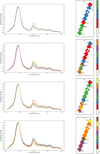 |
Fig. B.1 Average spectral profile (left) and spatial footprint (right) for clusters determined in the 3.2–3.6 μm region. Each cluster is labelled with a number (in an arbitrary manner). Shading and normalisation (left), and labels and masked pixels (right) are the same as in Fig. 3. |
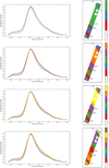 |
Fig. B.2 Average spectral profile (left) and spatial footprint (right) for clusters determined in the 5.95–6.6 μm region. Each cluster is labelled with a number (in an arbitrary manner). Shading and normalisation (left), and labels and masked pixels (right) are the same as in Fig. 4. |
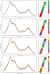 |
Fig. B.3 The average spectral profile (left) and spatial footprint (right) for clusters determined in the 7.25–8.95 μm region. Each cluster is labelled with a number (in an arbitrary manner). Shading and normalisation (left), and labels and masked pixels (right) are the same as in Fig. 5. |
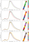 |
Fig. B.4 Average spectral profile (left) and spatial footprint (right) for clusters determined in the 10.9–11.63 μm region. Each cluster is labelled with a number (in an arbitrary manner). Shading and normalisation (left), and labels and masked pixels (right) are the same as in Fig. 6. |
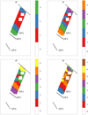 |
Fig. B.5 Spatial footprint of the MIRI MRS FOV is colour-coded by cluster assignment for three (top left), five (top right), six (bottom left) and seven (bottom right) clusters applied to the 4.9–13.2 μm region. Cluster assignment is calculated on the secondary round of clustering applied only to those pixels belonging to cluster 3 in the initial round of clustering (see Fig. 7). Cluster and FOV labels are the same as in Fig. 7. |
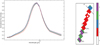 |
Fig. B.6 Average spectral profile (left) and spatial footprint (right) for clusters determined in the 3.2–3.36 μm region. Each cluster is labelled with a number (in an arbitrary manner). Shading and normalisation (left), and labels and masked pixels (right) are the same as in Fig. 3. |
Appendix C Further comparison of clustering results
Comparisons of the mean spectral profiles and cluster zone maps for each of the 7.25–8.95 and 3.2–3.6 μm regions with those based on clusters from the 10.9–11.63 μm region were also performed. The results from these experiments are given in Figs. C.1 and C.2, respectively.
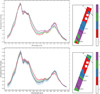 |
Fig. C.1 Average spectral profiles (left) for the 7.25–8.95 μm region obtained from clustering assignment based on the 7.25–8.95 μm region and the corresponding cluster zones (right) are given in the top two frames. The average spectral profiles (left) for the 7.25–8.95 μm region obtained from clustering assignment based on the 10.9–11.63 μm region and the corresponding cluster zones (right) are given in the bottom two frames. Cluster and FOV labels are the same as in Fig. 8. |
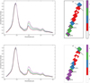 |
Fig. C.2 Average spectral profiles (left) for the 3.2–3.6 μm region obtained from clustering assignment based on the 3.2–3.6 μm region and the corresponding cluster zones (right) are given in the top two frames. The average spectral profiles (left) for the 3.2–3.6 μm region obtained from clustering assignment based on the 10.9–11.63 μm region and the corresponding cluster zones (right) are given in the bottom two frames. Note that due to differences in the spatial resolution of the NIRSpec and MIRI MRS datasets, there are small discrepancies in the pixel masks, such are apparent in the lower right panel. Cluster and FOV labels are the same as in Fig. 8. |
References
- Bauschlicher, Charles W.Jr., , Peeters, Els, Allamandola, Louis, J. 2009, ApJ, 697, 311 [NASA ADS] [CrossRef] [Google Scholar]
- Allamandola, L. J., Tielens, A. G. G. M., & Barker, J. R. 1985, ApJ, 290, L25 [Google Scholar]
- Allamandola, L. J., Tielens, A. G. G. M., & Barker, J. R. 1989, ApJS, 71, 733 [Google Scholar]
- Allamandola, L. J., Hudgins, D. M., & Sandford, S. A. 1999, ApJ, 511, L115 [Google Scholar]
- Andrews, H., Candian, A., & Tielens, A. 2016, A&A, 595, A23 [NASA ADS] [CrossRef] [EDP Sciences] [Google Scholar]
- Armus, L., Charmandaris, V., Bernard-Salas, J., et al. 2007, ApJ, 656, 148 [NASA ADS] [CrossRef] [Google Scholar]
- Bakes, E. L. O., & Tielens, A. G. G. M. 1994, ApJ, 427, 822 [NASA ADS] [CrossRef] [Google Scholar]
- Banerjee, S., Choudhary, A., & Pal, S. 2015, in 2015 IEEE International WIE Conference on Electrical and Computer Engineering (WIECON-ECE), IEEE, 168–172 [CrossRef] [Google Scholar]
- Bangoria Bhoomi, M. 2014, Int. J. Comput. Sci. Inf. Technol., 5, 876 [Google Scholar]
- Barker, J. R., Allamandola, L. J., & Tielens, A. G. G. M. 1987, ApJ, 315, L61 [NASA ADS] [CrossRef] [Google Scholar]
- Baron, D. 2019, arXiv e-prints, [arXiv: 1904.07248] [Google Scholar]
- Bauschlicher, Charles W., J., Peeters, E., & Allamandola, L. J. 2008, ApJ, 678, 316 [NASA ADS] [CrossRef] [Google Scholar]
- Bernard-Salas, J., Habart, E., Arab, H., et al. 2012, A&A, 538, A37 [NASA ADS] [CrossRef] [EDP Sciences] [Google Scholar]
- Berné, O., Joblin, C., Deville, Y., et al. 2007, A&A, 469, 575 [NASA ADS] [CrossRef] [EDP Sciences] [Google Scholar]
- Berné, O., Habart, É., Peeters, E., et al. 2022, PASP, 134, 054301 [CrossRef] [Google Scholar]
- Bernstein, M. P., Sandford, S. A., & Allamandola, L. J. 1996, ApJ, 472, L127 [NASA ADS] [CrossRef] [Google Scholar]
- Boersma, C., Rubin, R. H., & Allamandola, L. J. 2012, ApJ, 753, 168 [NASA ADS] [CrossRef] [Google Scholar]
- Boersma, C., Bregman, J. D., & Allamandola, L. J. 2013, ApJ, 769, 117 [NASA ADS] [CrossRef] [Google Scholar]
- Boersma, C., Bregman, J., & Allamandola, L. J. 2014, ApJ, 795, 110 [NASA ADS] [CrossRef] [Google Scholar]
- Boersma, C., Bregman, J., & Allamandola, L. J. 2016, ApJ, 832, 51 [NASA ADS] [CrossRef] [Google Scholar]
- Boissel, P., Joblin, C., & Pernot, P. 2001, A&A, 373, L5 [NASA ADS] [CrossRef] [EDP Sciences] [Google Scholar]
- Böker, T., Arribas, S., Lützgendorf, N., et al. 2022, A&A, 661, A82 [NASA ADS] [CrossRef] [EDP Sciences] [Google Scholar]
- Bregman, J., & Temi, P. 2005, ApJ, 621, 831 [CrossRef] [Google Scholar]
- Bregman, J. D., Allamandola, L. J., Tielens, A. G. G. M., Geballe, T. R., & Witteborn, F. C. 1989, ApJ, 344, 791 [NASA ADS] [CrossRef] [Google Scholar]
- Buragohain, M., Pathak, A., Sakon, I., & Onaka, T. 2020, ApJ, 892, 11 [NASA ADS] [CrossRef] [Google Scholar]
- Candian, A., Sarre, P. J., & Tielens, A. G. G. M. 2014, ApJ, 791, L10 [CrossRef] [Google Scholar]
- Cesarsky, D., Jones, A. P., Lequeux, J., & Verstraete, L. 2000, A&A, 358, 708 [NASA ADS] [Google Scholar]
- Chown, R., Sidhu, A., Peeters, E., et al. 2024, A&A, 685, A75 (Paper IV) [NASA ADS] [CrossRef] [EDP Sciences] [Google Scholar]
- Cohen, M., Tielens, A. G. G. M., Bregman, J., et al. 1989, ApJ, 341, 246 [NASA ADS] [CrossRef] [Google Scholar]
- Cuadrado, S., Salas, P., Goicoechea, J. R., et al. 2019, A&A, 625, L3 [NASA ADS] [CrossRef] [EDP Sciences] [Google Scholar]
- Davies, A., Serjeant, S., & Bromley, J. M. 2019, MNRAS, 487, 5263 [NASA ADS] [CrossRef] [Google Scholar]
- Di, J., & Gou, X. 2018, J. Comput., 13, 588 [CrossRef] [Google Scholar]
- Elliott, K. H., & Meaburn, J. 1974, Ap&SS, 28, 351 [NASA ADS] [CrossRef] [Google Scholar]
- Forgy, E. W. 1965, Biometrics, 21, 768 [Google Scholar]
- Foschino, S., Berné, O., & Joblin, C. 2019, A&A, 632, A84 [EDP Sciences] [Google Scholar]
- Galliano, F., Madden, S. C., Tielens, A. G. G. M., Peeters, E., & Jones, A. P. 2008, ApJ, 679, 310 [Google Scholar]
- Geballe, T. R., Tielens, A. G. G. M., Allamandola, L. J., Moorhouse, A., & Brand, P. W. J. L. 1989, ApJ, 341, 278 [NASA ADS] [CrossRef] [Google Scholar]
- Geers, V., Augereau, J.-C., Pontoppidan, K., et al. 2006, A&A, 459, 545 [NASA ADS] [CrossRef] [EDP Sciences] [Google Scholar]
- Genzel, R., Lutz, D., Sturm, E., et al. 1998, ApJ, 498, 579 [Google Scholar]
- Goicoechea, J. R., Teyssier, D., Etxaluze, M., et al. 2015, ApJ, 812, 75 [Google Scholar]
- Goicoechea, J. R., Pety, J., Cuadrado, S., et al. 2016, Nature, 537, 207 [Google Scholar]
- Goicoechea, J. R., Cuadrado, S., Pety, J., et al. 2017, A&A, 601, A9 [Google Scholar]
- Habart, E., Le Gal, R., Alvarez, C., et al. 2023, A&A, 673, A149 [NASA ADS] [CrossRef] [EDP Sciences] [Google Scholar]
- Habart, É., Peeters, E., Berné, O., et al. 2024, A&A, 685, A73 (Paper II) [NASA ADS] [CrossRef] [EDP Sciences] [Google Scholar]
- Herrmann, F., Madden, S. C., Nikola, T., et al. 1997, ApJ, 481, 343 [CrossRef] [Google Scholar]
- Hogerheijde, M. R., Jansen, D. J., & van Dishoeck, E. F. 1995, A&A, 294, 792 [NASA ADS] [Google Scholar]
- Hony, S., Van Kerckhoven, C., Peeters, E., et al. 2001, A&A, 370, 1030 [CrossRef] [EDP Sciences] [Google Scholar]
- Joblin, C., Tielens, A. G. G. M., Geballe, T. R., & Wooden, D. H. 1996, ApJ, 460, L119 [NASA ADS] [CrossRef] [Google Scholar]
- Keller, L. D., Sloan, G., Forrest, W., et al. 2008, ApJ, 684, 411 [NASA ADS] [CrossRef] [Google Scholar]
- Knight, C., Peeters, E., Stock, D. J., Vacca, W. D., & Tielens, A. G. G. M. 2021, ApJ, 918, 8 [NASA ADS] [CrossRef] [Google Scholar]
- Knight, C., Peeters, E., Tielens, A. G. G. M., & Vacca, W. D. 2022a, MNRAS, 509, 3523 [Google Scholar]
- Knight, C., Peeters, E., Wolfire, M., & Stock, D. J. 2022b, MNRAS, 510, 4888 [CrossRef] [Google Scholar]
- Lai, T. S. Y., Smith, J. D. T., Baba, S., Spoon, H. W. W., & Imanishi, M. 2020, ApJ, 905, 55 [NASA ADS] [CrossRef] [Google Scholar]
- Lai, T. S. Y., Armus, L., Bianchin, M., et al. 2023, ApJ, 957, L26 [NASA ADS] [CrossRef] [Google Scholar]
- Laurens, G., Rabary, M., Lam, J., Peláez, D., & Allouche, A.-R. 2021, Theoret. Chem. Acc., 140, 66 [CrossRef] [Google Scholar]
- Leger, A., & Puget, J. L. 1984, A&A, 137, L5 [Google Scholar]
- Mackie, C. J. 2018, PhD thesis, University of Leiden, The Netherlands [Google Scholar]
- Mackie, C. J., Candian, A., Lee, T. J., & Tielens, A. G. G. M. 2022, JPCA, 126, 3198 [NASA ADS] [CrossRef] [Google Scholar]
- Maltseva, E., Mackie, C. J., Candian, A., et al. 2018, A&A, 610, A65 [NASA ADS] [CrossRef] [EDP Sciences] [Google Scholar]
- Matsuura, M., Bernard-Salas, J., Lloyd Evans, T., et al. 2014, MNRAS, 439, 1472 [NASA ADS] [CrossRef] [Google Scholar]
- Meng, Z., Zhang, Y., Liang, E., & Wang, Z. 2023, MNRAS, 525, L29 [NASA ADS] [CrossRef] [Google Scholar]
- Mori, T. I., Onaka, T., Sakon, I., et al. 2014, ApJ, 784, 53 [NASA ADS] [CrossRef] [Google Scholar]
- Moutou, C., Sellgren, K., Verstraete, L., & Léger, A. 1999, A&A, 347, 949 [Google Scholar]
- O’Dell, C., Henney, W., Abel, N., Ferland, G. J., & Arthur, S. 2008, AJ, 137, 367 [Google Scholar]
- O’Dell, C., Kollatschny, W., & Ferland, G. J. 2017, ApJ, 837, 151 [CrossRef] [Google Scholar]
- O’Dell, C. R., Abel, N. P., & Ferland, G. J. 2020, ApJ, 891, 46 [CrossRef] [Google Scholar]
- Ossenkopf, V., Röllig, M., Neufeld, D. A., et al. 2013, A&A, 550, A57 [NASA ADS] [CrossRef] [EDP Sciences] [Google Scholar]
- Pabst, C., Higgins, R., Goicoechea, J. R., et al. 2019, Nature, 565, 618 [NASA ADS] [CrossRef] [Google Scholar]
- Pabst, C. H. M., Goicoechea, J. R., Teyssier, D., et al. 2020, A&A, 639, A2 [NASA ADS] [CrossRef] [EDP Sciences] [Google Scholar]
- Pedregosa, F., Varoquaux, G., Gramfort, A., et al. 2011, J. Mach. Learn. Res., 12, 2825 [Google Scholar]
- Peeters, E., Hony, S., Van Kerckhoven, C., et al. 2002, A&A, 390, 1089 [NASA ADS] [CrossRef] [EDP Sciences] [Google Scholar]
- Peeters, E., Tielens, A. G. G. M., Allamandola, L. J., & Wolfire, M. G. 2012, ApJ, 747, 44 [NASA ADS] [CrossRef] [Google Scholar]
- Peeters, E., Bauschlicher, C. W., Allamandola, L. J., et al. 2017, ApJ, 836, 198 [NASA ADS] [CrossRef] [Google Scholar]
- Peeters, E., Berné, O., Habart, É., et al. 2024, A&A, 685, A74 (Paper III) [NASA ADS] [CrossRef] [EDP Sciences] [Google Scholar]
- Pilleri, P., Montillaud, J., Berné, O., & Joblin, C. 2012, A&A, 542, A69 [NASA ADS] [CrossRef] [EDP Sciences] [Google Scholar]
- Pilleri, P., Joblin, C., Boulanger, F., & Onaka, T. 2015, A&A, 577, A16 [NASA ADS] [CrossRef] [EDP Sciences] [Google Scholar]
- Pla, P., Wang, Y., Martín, F., & Alcamí, M. 2020, ApJ, 899, 18 [NASA ADS] [CrossRef] [Google Scholar]
- Puget, J. L., & Léger, A. 1989, ARA&A, 27, 161 [NASA ADS] [CrossRef] [Google Scholar]
- Rapacioli, M., Calvo, F., Spiegelman, F., Joblin, C., & Wales, D. J. 2005a, JPCA, 109, 2487 [NASA ADS] [CrossRef] [Google Scholar]
- Rapacioli, M., Joblin, C., & Boissel, P. 2005b, A&A, 429, 193 [NASA ADS] [CrossRef] [EDP Sciences] [Google Scholar]
- Rhea, C. L., Rousseau-Nepton, L., Prunet, S., et al. 2021, ApJ, 923, 169 [NASA ADS] [CrossRef] [Google Scholar]
- Ricca, A., Bauschlicher, Charles W., J., Boersma, C., Tielens, A. G. G. M., & Allamandola, L. J. 2012, ApJ, 754, 75 [NASA ADS] [CrossRef] [Google Scholar]
- Ricca, A., Roser, J. E., Boersma, C., Peeters, E., Maragkoudakis, A. 2024, ApJ, accepted [Google Scholar]
- Ristoski, P., Bizer, C., & Paulheim, H. 2015, J. Web Semant., 35, 142 [CrossRef] [Google Scholar]
- Rosenberg, M. J. F., Berné, O., Boersma, C., Allamandola, L. J., & Tielens, A. G. G. M. 2011, A&A, 532, A128 [NASA ADS] [CrossRef] [EDP Sciences] [Google Scholar]
- Rubin, R. H., Simpson, J. P., O’Dell, C. R., et al. 2011, MNRAS, 1526 [Google Scholar]
- Sadjadi, S., Zhang, Y., & Kwok, S. 2015, ApJ, 801, 34 [NASA ADS] [CrossRef] [Google Scholar]
- Salas, P., Oonk, J. B. R., Emig, K. L., et al. 2019, A&A, 626, A70 [NASA ADS] [CrossRef] [EDP Sciences] [Google Scholar]
- Salgado, F., Berné, O., Adams, J., et al. 2016, ApJ, 830, 118 [NASA ADS] [CrossRef] [Google Scholar]
- Savaresi, S. M., & Boley, D. L. 2001, in Proceedings of the 2001 SIAM International Conference on Data Mining, SIAM, 1 [Google Scholar]
- Schutte, W. A., Tielens, A. G. G. M., & Allamandola, L. J. 1993, ApJ, 415, 397 [NASA ADS] [CrossRef] [Google Scholar]
- Schroetter, I., Berné, O., Joblin, C., et al. 2024, A&A, 685, A78 (Paper VII) [NASA ADS] [CrossRef] [EDP Sciences] [Google Scholar]
- Selim, S. Z., & Ismail, M. A. 1984, IEEE Trans. Pattern Anal. Mach. Intell., PAMI-6, 81 [CrossRef] [Google Scholar]
- Sellgren, K. 1984, ApJ, 277, 623 [Google Scholar]
- Sellgren, K., Werner, M. W., & Dinerstein, H. L. 1983, ApJ, 271, L13 [CrossRef] [Google Scholar]
- Shannon, M. J., Stock, D. J., Peeters, E. 2016, ApJ, 824, 18 [NASA ADS] [CrossRef] [Google Scholar]
- Sidhu, A., Peeters, E., Cami, J., & Knight, C. 2021, MNRAS, 500, 177 [Google Scholar]
- Sidhu, A., Bazely, J., Peeters, E., & Cami, J. 2022, MNRAS, 511, 2186 [NASA ADS] [CrossRef] [Google Scholar]
- Sloan, G. C., Bregman, J. D., Geballe, T. R., Allamandola, L. J., & Woodward, E. 1997, ApJ, 474, 735 [NASA ADS] [CrossRef] [Google Scholar]
- Sloan, G., Jura, M., Duley, W., et al. 2007, ApJ, 664, 1144 [NASA ADS] [CrossRef] [Google Scholar]
- Steglich, M., Jäger, C., Huisken, F., et al. 2013, ApJS, 208, 26 [NASA ADS] [CrossRef] [Google Scholar]
- Steinbach, M., Karypis, G., & Kumar, V. 2000, A comparison of document clustering techniques, Tech. rep., The University of Minnesota Digital Conservancy [Google Scholar]
- Stock, D. J., & Peeters, E. 2017, ApJ, 837, 129 [NASA ADS] [CrossRef] [Google Scholar]
- Sundararajan, P., Tsuge, M., Baba, M., Sakurai, H., & Lee, Y.-P. 2019, J. Chem. Phys., 151 [Google Scholar]
- Tammour, A., Gallagher, S. C., Daley, M., & Richards, G. T. 2016, MNRAS, 459, 1659 [NASA ADS] [CrossRef] [Google Scholar]
- Tauber, J. A., Lis, D. C., Keene, J., Schilke, P., & Buettgenbach, T. H. 1995, A&A, 297, 567 [Google Scholar]
- Tielens, A. G. 2008, ARA&A, 46, 289 [NASA ADS] [CrossRef] [Google Scholar]
- Tielens, A. G. 2021, Molecular Astrophysics (Cambridge University Press) [CrossRef] [Google Scholar]
- Tielens, A. G. G. M., & Hollenbach, D. 1985, ApJ, 291, 747 [NASA ADS] [CrossRef] [Google Scholar]
- Tielens, A. G. G. M., Meixner, M. M., van der Werf, P. P., et al. 1993, Science, 262, 86 [NASA ADS] [CrossRef] [Google Scholar]
- van der Werf, P. P., Goss, W. M., & O’Dell, C. R. 2013, ApJ, 762, 101 [NASA ADS] [CrossRef] [Google Scholar]
- Van De Putte, D., Meshaka, R., Trahin, B., et al 2024, A&A, submitted (Paper VIII) [Google Scholar]
- van Diedenhoven, B., Peeters, E., Van Kerckhoven, C., et al. 2004, ApJ, 611, 928 [NASA ADS] [CrossRef] [Google Scholar]
- Verstraete, L., Puget, J., Falgarone, E., et al. 1996, A&A, 315, L337 [NASA ADS] [Google Scholar]
- Wang, J. Z., Wiederhold, G., Firschein, O., & Xin Wei, S. 1998, Int. J. Digit. Libr., 1, 311 [CrossRef] [Google Scholar]
- Wagner, D. R., Kim, H., & Saykally, R. J. 2000, ApJ, 545, 854 [CrossRef] [Google Scholar]
- Wyrowski, F., Schilke, P., Hofner, P., & Walmsley, C. M. 1997, ApJ, 487, L171 [NASA ADS] [CrossRef] [Google Scholar]
- Yang, X., Li, A., & Glaser, R. 2020, ApJS, 247, 1 [CrossRef] [Google Scholar]
- Zang, R. X., Peeters, E., & Boersma, C. 2019, ApJ, 887, 46 [NASA ADS] [CrossRef] [Google Scholar]
- Zhao, Y., Karypis, G., & Fayyad, U. 2005, Data Min. Knowl. Discov., 10, 141 [CrossRef] [Google Scholar]
DOI: 10.17909/pg4c-1737 and 10.17909/wqwy-p406
All Tables
Average silhouette scores and elbow points for each of the clustering experiments are given.
All Figures
|
Fig. 1 Schematic sketch of the anatomy of the Bar. The dimensions perpendicular to the bar are not to scale but are given at the bottom of the sketch. We also note that foreground material is not depicted. This includes a layer of ionised gas (O’Dell et al. 2020) and the Veil (e.g. Rubin et al. 2011; Boersma et al. 2012; van der Werf et al. 2013; Pabst et al. 2019, 2020). Figure taken from Peeters et al. (2024). |
| In the text | |
|
Fig. 2 PDRs4All FOVs for both NIRSpec IFU and MIRI MRS datasets are illustrated with the solid and dashed white lines, respectively. The FOVs are overlaid on a composite NIRCam image of the Bar constructed from PDRs4All imaging data (Habart et al. 2024), where red, green, and blue are encoded as F335M (3.3 μm aromatic infrared band emission), F470N-F444W (H2 emission), and F187N (Paschen α emission), respectively. The location of the ionising source, θ1 Ori C, is shown with the white circle in the top right corner of the left panel. The two proplyds, 203–504 and 203–506, are outlined with black circles. Figure adapted from Chown et al. (2024). |
| In the text | |
|
Fig. 3 Average spectral profile (left) and spatial footprint (right) for all clusters determined in the 3.2–3.6 μm region. Each cluster is labelled with an integer numbered 1 through 4 (in an arbitrary manner). Left panel: The shaded regions around each profile illustrate one standard deviation from the mean profile intensity at a given wavelength value. Each spectrum is normalised to its peak 3.3 μm intensity for visualisation purposes. Right panel: The spatial footprint of the NIRSpec FOV colour-coded by cluster assignment. Any masked pixels or those that have been otherwise masked out are labelled with 0. The black, dashed lines indicate the locations of the ionisation front (IF) and the three dissociation fronts (DF 1, DF 2 and DF 3) as defined in Peeters et al. (2024) using nomenclature established in Habart et al. (2024). |
| In the text | |
|
Fig. 4 Average spectral profile (left) and spatial footprint (right) for all clusters determined in the 5.95–6.6 μm region. Each cluster is labelled with an integer numbered 1 through 4 (in an arbitrary manner). Left panel: The shaded regions around each profile illustrate one standard deviation from the mean profile intensity at a given wavelength value. Each spectrum is normalised to its peak 6.2 μm intensity for visualisation purposes. Right panel: The spatial footprint of the MIRI MRS FOV is colour-coded by cluster assignment. Any masked pixels or those that have been otherwise masked out are labelled with a 0. The black, dashed lines indicate the locations of the IF, DF 1, DF 2 and DF 3. |
| In the text | |
|
Fig. 5 Average spectral profile (left) and spatial footprint (right) for all clusters determined in the 7.25–8.95 μm region. Each cluster is labelled with an integer numbered 1 through 4 (in an arbitrary manner). Left panel: the shaded regions around each profile illustrate one standard deviation from the mean profile intensity at a given wavelength value. Each spectrum is normalised to its peak 7.7 μm intensity for visualisation purposes. Right panel: the spatial footprint of the MIRI MRS FOV is colour-coded by cluster assignment. Any masked pixels or those that have been otherwise masked out are labelled with a 0. The black, dashed lines indicate the locations of the IF, DF 1, DF 2 and DF 3. |
| In the text | |
|
Fig. 6 Average spectral profile (left) and spatial footprint (right) for all clusters determined in the 10.9–11.63 μm region. Each cluster is labelled with an integer numbered 1 through 4 (in an arbitrary manner). Left panel: the shaded regions around each profile illustrate one standard deviation from the mean profile intensity at a given wavelength value. Each spectrum is normalised to its peak 11.2 μm intensity for visualisation purposes. Right panel: the spatial footprint of the MIRI MRS FOV is colour-coded by cluster assignment. Any masked pixels or those that have been otherwise masked out are labelled with a 0. The black, dashed lines indicate the locations of the IF, DF 1, DF 2 and DF 3. |
| In the text | |
|
Fig. 7 Spatial footprint of the MIRI MRS FOV is colour-coded by cluster assignment calculated on an initial (left) and secondary (right) round of clustering on all spectral features in the MIRI MRS dataset shortwards of 13.2 μm. The secondary round of clustering was applied only to those pixels belonging to cluster 1 in the initial round of clustering that largely coincide with the atomic PDR. Clusters are labelled 1 through 4 (in an arbitrary manner) and masked pixels are labelled 0. The black, dashed lines indicate the locations of the IF, DF 1, DF 2 and DF 3. |
| In the text | |
|
Fig. 8 Average spectral profiles (left) for the 6.2 μm band obtained from clustering assignment based on the 5.95–6.6 μm region and the corresponding cluster zones (right) are given in the top two frames. The average spectral profiles (left) for the 6.2 μm band obtained from clustering assignment based on the 10.9–11.63 μm region and the corresponding cluster zones (right) are given in the bottom two frames. Left panels: the shaded regions around each profile illustrate one standard deviation from the mean profile intensity at a given wavelength value. Each spectrum is normalised to the peak 6.2 μm intensity for visualisation purposes. Right panels: the spatial footprint of the MIRI MRS FOV colour-coded by cluster assignment. Any masked pixels or those that have been otherwise masked out are labelled as 0. The black, dashed lines illustrate the locations of the ionisation front (IF) and the three dissociation fronts (DF 1, DF 2 and DF 3) as defined in Peeters et al. (2024) using nomenclature established in Habart et al. (2024). |
| In the text | |
|
Fig. 9 Linear combinations of the class A11.2 profile and a ‘secondary component’ that recover the ‘intermediate’ 11.2 μm profiles of clusters 3 (left) and 2 (right) from the 10.9–11.63 μm wavelength region (see Sect. 5.4 for details). The cluster profile is shown in blue and green in the left and right panel respectively. The dashed purple line represents the scaled class A11.2 profile given by cluster 4, the dashed orange line is the secondary component, and the bright magenta line represents the linear combination of these two components. We note that the small undulations in the red wing of the profiles are residual fringes present due to incomplete fringe removal. |
| In the text | |
|
Fig. 10 Spatial morphology of the 11.25/11.207 intensity ratio (i.e. the ratio of the surface brightness at 11.25 μηι to the surface brightness at 11.207 μm after continuum subtraction). The 11.25 μm component dominates over the 11.207 μm component in the deeper regions of the PDR, past DF 1, especially in DF 3. |
| In the text | |
|
Fig. A.1 Distortion scores for clustering applied in the 3.2–3.6, 5.95–6.6, 7.25–8.95, and 10.9–11.63 μm region plotted as a function of the number of clusters used. The inflection point, or ‘elbow’, in the distortion curve is highlighted with the dashed black line. As is shown, four clusters are optimal for each wavelength regime. |
| In the text | |
|
Fig. A.2 Distortion scores for clustering on the first (left) and second (right) round of clustering for the 4.9–13.2 μm region in the MIRI MRS dataset as a function of the number of clusters used. The inflection point, or ‘elbow’, in the distortion curve is highlighted with the dashed black line. In the case of the first round of clustering across the entire, cleaned MIRI MRS footprint, four clusters are optimal. In the case of the clustering focused to pixels belonging to the cluster coincident with the atomic PDR, five clusters are optimal. |
| In the text | |
|
Fig. B.1 Average spectral profile (left) and spatial footprint (right) for clusters determined in the 3.2–3.6 μm region. Each cluster is labelled with a number (in an arbitrary manner). Shading and normalisation (left), and labels and masked pixels (right) are the same as in Fig. 3. |
| In the text | |
|
Fig. B.2 Average spectral profile (left) and spatial footprint (right) for clusters determined in the 5.95–6.6 μm region. Each cluster is labelled with a number (in an arbitrary manner). Shading and normalisation (left), and labels and masked pixels (right) are the same as in Fig. 4. |
| In the text | |
|
Fig. B.3 The average spectral profile (left) and spatial footprint (right) for clusters determined in the 7.25–8.95 μm region. Each cluster is labelled with a number (in an arbitrary manner). Shading and normalisation (left), and labels and masked pixels (right) are the same as in Fig. 5. |
| In the text | |
|
Fig. B.4 Average spectral profile (left) and spatial footprint (right) for clusters determined in the 10.9–11.63 μm region. Each cluster is labelled with a number (in an arbitrary manner). Shading and normalisation (left), and labels and masked pixels (right) are the same as in Fig. 6. |
| In the text | |
|
Fig. B.5 Spatial footprint of the MIRI MRS FOV is colour-coded by cluster assignment for three (top left), five (top right), six (bottom left) and seven (bottom right) clusters applied to the 4.9–13.2 μm region. Cluster assignment is calculated on the secondary round of clustering applied only to those pixels belonging to cluster 3 in the initial round of clustering (see Fig. 7). Cluster and FOV labels are the same as in Fig. 7. |
| In the text | |
|
Fig. B.6 Average spectral profile (left) and spatial footprint (right) for clusters determined in the 3.2–3.36 μm region. Each cluster is labelled with a number (in an arbitrary manner). Shading and normalisation (left), and labels and masked pixels (right) are the same as in Fig. 3. |
| In the text | |
|
Fig. C.1 Average spectral profiles (left) for the 7.25–8.95 μm region obtained from clustering assignment based on the 7.25–8.95 μm region and the corresponding cluster zones (right) are given in the top two frames. The average spectral profiles (left) for the 7.25–8.95 μm region obtained from clustering assignment based on the 10.9–11.63 μm region and the corresponding cluster zones (right) are given in the bottom two frames. Cluster and FOV labels are the same as in Fig. 8. |
| In the text | |
|
Fig. C.2 Average spectral profiles (left) for the 3.2–3.6 μm region obtained from clustering assignment based on the 3.2–3.6 μm region and the corresponding cluster zones (right) are given in the top two frames. The average spectral profiles (left) for the 3.2–3.6 μm region obtained from clustering assignment based on the 10.9–11.63 μm region and the corresponding cluster zones (right) are given in the bottom two frames. Note that due to differences in the spatial resolution of the NIRSpec and MIRI MRS datasets, there are small discrepancies in the pixel masks, such are apparent in the lower right panel. Cluster and FOV labels are the same as in Fig. 8. |
| In the text | |
Current usage metrics show cumulative count of Article Views (full-text article views including HTML views, PDF and ePub downloads, according to the available data) and Abstracts Views on Vision4Press platform.
Data correspond to usage on the plateform after 2015. The current usage metrics is available 48-96 hours after online publication and is updated daily on week days.
Initial download of the metrics may take a while.