| Issue |
A&A
Volume 681, January 2024
|
|
|---|---|---|
| Article Number | A47 | |
| Number of page(s) | 29 | |
| Section | Interstellar and circumstellar matter | |
| DOI | https://doi.org/10.1051/0004-6361/202347535 | |
| Published online | 08 January 2024 | |
Mid-infrared evidence for iron-rich dust in the multi-ringed inner disk of HD 144432★
1
HUN-REN Research Centre for Astronomy and Earth Sciences, Konkoly Observatory,
Konkoly-Thege Miklós út 15–17,
1121
Budapest,
Hungary
2
CSFK, MTA Centre of Excellence,
Konkoly-Thege Miklós út 15–17,
1121
Budapest,
Hungary
e-mail: varga.jozsef@csfk.org
3
Leiden Observatory, Leiden University,
PO Box 9513,
2300 RA
Leiden,
The Netherlands
4
Institute for Mathematics, Astrophysics and Particle Physics, Radboud University,
PO Box 9010,
MC 62, 6500 GL
Nijmegen,
The Netherlands
5
SRON Netherlands Institute for Space Research,
Niels Bohrweg 4,
2333 CA
Leiden,
The Netherlands
6
Anton Pannekoek Institute for Astronomy, University of Amsterdam,
Science Park 904,
1090 GE
Amsterdam,
The Netherlands
7
Max-Planck-Institut für Astronomie,
Königstuhl 17,
69117
Heidelberg,
Germany
8
Université Côte d’Azur, Observatoire de la Côte d’Azur, CNRS,
Laboratoire Lagrange,
France
9
Univ. Grenoble Alpes, CNRS, IPAG,
38000
Grenoble,
France
10
Institute of Theoretical Physics and Astrophysics, University of Kiel,
Leibnizstr. 15,
24118
Kiel,
Germany
11
ELTE Eötvös Loránd University, Institute of Physics,
Pázmány Péter sétány 1/A,
1117
Budapest,
Hungary
12
Visiting astronomer, Laboratoire Lagrange, Université Côte d’Azur, Observatoire de la Côte d’Azur, CNRS,
Boulevard de l’Observatoire, CS 34229,
06304
Nice Cedex 4,
France
13
Max Planck Institute for Extraterrestrial Physics,
Giessenbachstrasse,
85741
Garching bei München,
Germany
14
INAF-Osservatorio Astronomico di Capodimonte,
via Moiariello 16,
80131
Napoli,
Italy
15
Institut de Recherche en Astrophysique et Planétologie, Université de Toulouse, UT3-PS, OMP, CNRS,
9 Av. du Colonel Roche,
31028
Toulouse Cedex 4,
France
16
NASA Goddard Space Flight Center, Astrophysics Division,
Greenbelt,
MD,
20771,
USA
17
Max-Planck-Institut für Radioastronomie,
Auf dem Hügel 69,
53121,
Bonn,
Germany
18
STAR Institute, University of Liège,
Liège,
Belgium
19
I. Physikalisches Institut, Universität zu Köln,
Zülpicher Str. 77,
50937
Köln,
Germany
20
CENTRA, Centro de Astrofísica e Gravitação, IST, Universidade de Lisboa, 1049-001 Lisboa, Portugal and Faculdade de Engenharia, Universidade do Porto,
Rua Dr. Roberto Frias,
4200-465
Porto,
Portugal
21
AIM, CEA, CNRS, Université Paris-Saclay, Université Paris-Diderot,
Sorbonne Paris-Cité,
91191
Gif-sur-Yvette,
France
22
European Southern Observatory,
Karl-Schwarzschild-Straße 2,
85748
Garching,
Germany
23
Space Research Institute, Austrian Academy of Sciences,
Schmiedlstr. 6,
8042
Graz,
Austria
Received:
22
July
2023
Accepted:
9
November
2023
Context. Rocky planets form by the concentration of solid particles in the inner few au regions of planet-forming disks. Their chemical composition reflects the materials in the disk available in the solid phase at the time the planets were forming. Studying the dust before it gets incorporated in planets provides a valuable diagnostic for the material composition.
Aims. We aim to constrain the structure and dust composition of the inner disk of the young Herbig Ae star HD 144432, using an extensive set of infrared interferometric data taken by the Very Large Telescope Interferometer (VLTI), combining PIONIER, GRAVITY, and MATISSE observations.
Methods. We introduced a new physical disk model, TGMdust, to image the interferometric data, and to fit the disk structure and dust composition. We also performed equilibrium condensation calculations with GGchem to assess the hidden diversity of minerals occurring in a planet-forming disk such as HD 144432.
Results. Our best-fit model has three disk zones with ring-like structures at 0.15, 1.3, and 4.1 au. Assuming that the dark regions in the disk at ~0.9 au and at ~3 au are gaps opened by planets, we estimate the masses of the putative gap-opening planets to be around a Jupiter mass. We find evidence for an optically thin emission (τ < 0.4) from the inner two disk zones (r < 4 au) at λ > 3 µm. Our silicate compositional fits confirm radial mineralogy gradients, as for the mass fraction of crystalline silicates we get around 61% in the innermost zone (r < 1.3 au), mostly from enstatite, while only ~20% in the outer two zones. To identify the dust component responsible for the infrared continuum emission, we explore two cases for the dust composition, one with a silicate+iron mixture and the other with a silicate+carbon one. We find that the iron-rich model provides a better fit to the spectral energy distribution. Our GGchem calculations also support an iron-rich and carbon-poor dust composition in the warm disk regions (r < 5 au, T > 300 K).
Conclusions. We propose that in the warm inner regions (r < 5 au) of typical planet-forming disks, most if not all carbon is in the gas phase, while iron and iron sulfide grains are major constituents of the solid mixture along with forsterite and enstatite. Our analysis demonstrates the need for detailed studies of the dust in inner disks with new mid-infrared instruments such as MATISSE and JWST/MIRI.
Key words: protoplanetary disks / techniques: interferometric / stars: pre-main sequence / stars: individual: HD 144432 / stars: variables: T Tauri, Herbig Ae/Be / planets and satellites: formation
© The Authors 2024
 Open Access article, published by EDP Sciences, under the terms of the Creative Commons Attribution License (https://creativecommons.org/licenses/by/4.0), which permits unrestricted use, distribution, and reproduction in any medium, provided the original work is properly cited.
This article is published in open access under the Subscribe to Open model. Subscribe to A&A to support open access publication.
1 Introduction
Young low- and intermediate-mass pre-main-sequence stars are often surrounded by a gas and dust disk. This disk forms early in the star formation process as a result of angular momentum conservation, as matter from the collapsing molecular cloud core accretes onto the forming protostar. Recent observations with high-angular resolution facilities – for example, the Atacama Large Millimeter/Submillimeter Array (ALMA) and the Spectro-Polarimetric High-contrast Exoplanet REsearch at the Very Large Telescope (VLT/SPHERE) – have revealed a rich variety of substructures in those disks (e.g., ALMA Partnership 2015; Andrews et al. 2018; Huang et al. 2018; Avenhaus et al. 2018; Boccaletti et al. 2020). These observations show rings, gaps, spiral arms, crescents, and clumps. This is accompanied with strong observational evidence that planets form and evolve in those disks (Marois et al. 2008; Keppler et al. 2018; Müller et al. 2018; Teague et al. 2018; Pinte et al. 2019). Planet formation may start very soon after the formation of the disk, as evidenced by structures detected in very young disks (<2 Myr) using high-resolution images at millimeter wavelengths (ALMA Partnership 2015; Sheehan & Eisner 2018; Segura-Cox et al. 2020; Nakatani et al. 2020; Sheehan et al. 2020, 2022).
These observations are put into context using thermochemical and hydrodynamical disk models that describe the changes expected in the disk structure and chemical composition of the gas and the solids as a result of planet formation (e.g., Kley & Nelson 2012; Flock et al. 2015; Woitke et al. 2018). Key questions to address are how to link the observed diversity of planetary systems to the properties of the disks in which they form; what are the processes that determine the composition of exoplanets and their atmospheres; and how can we constrain the chemical composition of the rocky planets that form from the refractory dust in the inner regions of disks.
As the disk evolves, the small (sub-µm sized) and mostly amorphous silicate dust grains that are accreted from the molecular cloud experience grain growth through coagulation and begin to settle toward the midplane, and, once reaching a critical size that depends on the local gas pressure, drift inward toward the star (Testi et al. 2014). While in the outer disk grain growth dominates, in the dense inner disk grain-grain collisions result in a collisional equilibrium, which may include planetesimalsized bodies. As the temperature increases inward, the chemical composition and lattice structure of the grains are modified, eventually leading to annealed, crystalline grains (Bouwman et al. 2001; Henning 2010). While irradiation from the central star heats up the disk surface, viscous heating due to accretion acts in the midplane. Both processes cause part of the dust to constantly evaporate and reform (Min et al. 2011). Gas phase condensation of solid material in the inner disk regions provides a source of freshly condensed crystalline material that are mixed in with the grains that are accreted from the molecular cloud (Sargent et al. 2009; Matter et al. 2020).
These processes tend to produce a radial distribution of silicate grains with a gradient in size and crystallinity (van Boekel et al. 2004; Varga et al. 2018). The opening of disk gaps and associated gas pressure bumps (Ruge et al. 2016; Dullemond et al. 2018) can lead to size sorting and thus substantially different spatial distributions of large and small grains in the disk (Pinilla et al. 2012). In addition, parent body processing followed by a collisional release of small grains may also modify the chemical composition of the grains in the inner disk (Thébault & Augereau 2007). Finally, episodic eruptions (Ábrahám et al. 2009), photoevaporative winds (Owen et al. 2011), and local heating processes (for instance, related to the formation of gas giant planets, or electrical discharges in the disk) also affect the nature and spatial distribution of the small grains (Pilipp et al. 1998; Desch & Cuzzi 2000; Harker & Desch 2002).
Spectral analysis can uncover the mineral buildup of the dust in planet-forming disks (van Boekel et al. 2005; Juhász et al. 2010; Olofsson et al. 2010), thus providing clues about the composition of future planets that formed from that material to be compared with the Solar System. Silicate dust grains in the size range up to an ~5 µm radius are easily detected in the surface layers of passively heated disks, because of the strong vibrational resonances at infrared (IR) wavelengths that cause emission bands and allow a measure of their chemical composition and size (e.g., Molster & Waters 2003). Observations have indeed shown the presence of µm-sized grains in the disk surface that are substantially larger than those found in the interstellar medium, and of crystalline silicates such as olivines and pyroxenes with very low Fe/Mg ratios, consistent with forsterite (Mg2SiO4) and enstatite (MgSiO3; Henning 2010). These minerals are also abundant in the inner Solar System bodies, as an example, Mg, Si, and O constitute 59% of the mass of Earth (Morgan & Anders 1980). However, the single most abundant element present in the inner Solar System planets is Fe (e.g., it makes up 32% of the mass of Earth, Morgan & Anders 1980), which is mostly concentrated in the cores of the planets. This implies that during the formation of planets, a large reservoir of iron-containing dust was available. Yet, the detection of iron in the interstellar and circumstellar dust proves to be elusive1. Metallic iron does not show any conspicuous spectral features at optical and IR wavelengths, in contrast to silicates. The same applies for amorphous carbon dust, which is also presumed to be present in the cosmic dust (e.g., Henning & Salama 1998; Tielens 2022).
In this paper one of our main aims is to attempt to constrain the solid iron content of a planet-forming disk, using IR photometric and spectro-interferometric observations. For that we analyzed the spectral fingerprints of the different dust species, aiming to constrain their mass ratios. The novel aspect in this work is that we performed a consistent modeling of high angular resolution IR interferometric data that enables us to uncover the disk structure at sub-au resolution, and at the same time determine the composition and radial distribution of the dust. Spatially resolving the warm inner parts of the disk (<10 au) where the relevant dust emission features originate is a key aspect, because it enables a more direct inference of the optical properties of the solids, that can be compared to optical data of minerals from laboratory experiments (Dorschner et al. 1995; Jäger et al. 1998a).
Here we study the planet-forming disk around HD 144432 A, a nearby Herbig Ae star belonging to the Upper Sco subgroup of the Sco-Cen OB association (Galli et al. 2018; Luhman & Esplin 2020), at a distance of 154.1 pc (Bailer-Jones et al. 2021), with a spectral type of A9/F0V (Houk 1982). Müller et al. (2011) showed that HD 144432 is a hierarchical triple system, consisting of the A-type primary, and a close binary system located 1″.47 (227 au) away. The close binary pair, HD 144432 B and C has a separation of 0″.1 (15 au). Components B and C are T Tauri type stars of spectral type K7V and M1V, respectively, and the triple system seems to be coeval with an age of 6 ± 3 Myr (Müller et al. 2011). HD 144432 has a prominent silicate spectral emission feature in the N band (8–13 µm), with one of the highest peak-to-continuum ratios (~4) observed so far (van Boekel et al. 2005). From a comparison of ISOPHOT-S and Spitzer InfraRed Spectrograph (IRS) spectra of the object, Kóspál et al. (2012) pointed out that the N band silicate feature of HD 144432 is variable. van Boekel et al. (2004) presented N band (8–13 µm) spectrointerferometric observations of HD 144432 from the VLTI/MIDI instrument. The authors found a radial mineralogy gradient in the disk, where the region within r ~ 2 au is richer in crystalline silicate grains, compared to the rest of the disk.
Chen et al. (2012) studied near-IR (H and K bands) VLTI/AMBER interferometric observations of HD 144432. Using a geometric ring model they found a nearly face-on disk (inclination <28º) with a K band ring radius of 0.17 ± 0.01 au, which may be consistent with the location of the dust sublimation radius. They also needed a spatially extended halo component to fit their data. In their subsequent paper (Chen et al. 2016a), they presented radiative transfer simulations with RADMC-3D using H (IOTA, AMBER), K (Keck Interferometer, AMBER), and N band (MIDI) data. Their best-fit model features an optically thin inner disk component between 0.2 and 0.3 au, and an optically thick outer disk between 1.4 and 10 au. They conclude that the disk of HD 144432 has a gap-like discontinuity at around 1 au radius, characteristic of pre-transitional disks. Such disks are thought to represent an evolutionary step between an earlier stage where optically thick material fills the entire warm region (≲10 au), and the later transitional disk stage where the warm disk region is mostly cleared of dust. Monnier et al. (2017) were not able to detect the disk of HD 144432 in H band scattered light (using GPI), concluding that the nearby companion may truncate the outer disk. HD 144432 was part of a VLT/SPHERE survey of self-shadowed disks (Garufi et al. 2022). The authors suggest that the disk is detected out to 0.25″ (~40 au), and that the strong asymmetry in the polarimetric image may be because of shadowing (see Fig. 2, and page 5 therein).
In this paper, we model new L, M, and N band VLTI/MATISSE and K band VLTI/GRAVITY interferometric observations of HD 144432, complemented with archival data from VLTI/PIONIER (H band). To our knowledge, this is the most complete IR interferometric data-set on a young stellar object analyzed so far, in terms of wavelength coverage, ranging between 1.6–13 µm. We apply a new flat disk temperature gradient model with simple radiative transfer to fit the data, that is able to reveal disk substructures, and constrain the dust composition. The paper is structured as follows: in Sect. 2 we describe the observations and data processing, in Sect. 3 we present our modeling approach, in Sect. 4 we show our results, followed by a discussion and summary in Sects. 5 and 6, respectively.
Overview of VLTI observations of HD 144432 used in our work.
2 Observations and data processing
European Southern Observatory’s (ESO) Very Large Telescope Interferometer (VLTI) is located at Paranal Observatory, Chile. Currently VLTI has three instruments: PIONIER, working in H band (1.6 µm); GRAVITY, working in K band (2.2 µm); and MATISSE, working in L (2.8–4 µm), M (4.6–5 µm), and N (8– 13 µm) bands. All of these instruments combine the light of four telescopes, either of the 8.2 m diameter Unit Telescopes (UTs), or of the 1.8 m diameter Auxiliary Telescopes (ATs). Using interferometric beam combination, VLTI instruments sample the visibility function, a complex quantity, which is the Fourier-transform of the object’s brightness distribution on the sky. We collected a large set of VLTI data on HD 144432 partly from our observations, partly from the Optical interferometry DataBase (OiDB) at the Jean-Marie Mariotti Center. Table 1 shows the overview of the VLTI observations used. Additionally, we collected archival IR photometric and spectroscopic data using the VizieR catalog access tool.
VLTI instruments provide spectrally resolved measurements. As the probed IR bands are quite broad, the angular resolution (ϑ) varies considerably over a band, modulating the spectral response. Additionally, spectral modulations can arise due to well-resolved structures in the disk. In the interferometric data, those spatial signatures are mixed with spectral emission or absorption features of the dust grains. A key aspect in our analysis is to disentangle the spatial signatures from true spectral information.
The angular resolution of VLTI instruments depends on the wavelength and the actual baseline lengths of the observations. The fixed UT array has a baseline range of 46–130 m, while, as of 2023, the movable ATs can be positioned to three configurations: small (11–34 m), medium (40–104 m), and large (58–132 m). The approximate angular resolution2 at long baselines (100–130 m) is 2 mas for PIONIER, 3 mas for GRAVITY, 4.5 mas for MATISSE L band (at 3.5 µm), and 14 mas for MATISSE N band (at 10 µm). These numbers translate to physical scales in the range of 0.3–2 au at the distance of our object.
2.1 MATISSE observations and data processing
We observed HD 144432 with MATISSE (Lopez et al., in prep.) between 2019 and 2022 in the frame of our Guaranteed Time Observing (GTO) program for surveying young stellar objects (YSOs). Data from 2019 were taken using the standard instrument mode (MATISSE standalone), while the 2022 data were taken using GRA4MAT. GRA4MAT (Woillez et al., in prep., GRAVITY for MATISSE) is a new instrument mode, which uses the fringe tracker of the GRAVITY instrument (GRAVITY Collaboration 2017) to stabilize the MATISSE fringes. This allows us to have longer integration time (on the order of seconds), in order to reach higher signal-to-noise ratio (S/N). In contrast, the integration time of MATISSE standalone is limited by the coherence time of the atmosphere, typically ~0.1 s in L band. We reduced and calibrated the data, and selected a set of data products to be used in this work. The selection was necessary to ensure that only good quality data (taken in good atmospheric conditions, and without technical issues) ended up in our final data set for modeling. Table 1 lists those data sets. The selected data sets were observed at seeing values ranging between 0.4″ and 1.3″, and atmospheric coherence time (τ0) values between 2.8 and 16.8 ms.
We used versions 1.5.0 (for the 2019 data) and 1.5.8 (for the 2022 data) of the standard MATISSE data reduction pipeline (DRS; Millour et al. 2016) to process the data3. Additional processing steps, like Beam Commuting Device (BCD) calibration and flux calibration was performed using the MATISSE tools python software package4. Final processing (averaging and merging different data types to a final OIFITS file) was done using our own python tool. We applied the same data processing workflow as in Varga et al. (2021). For more details, we refer to Sect. 3.1 in that work. Each calibrated data set contains the following: spectrally resolved visibilities on six baselines, closure phases on 4 baseline triplets, flux-calibrated correlated spectra5 on six baselines, and a flux-calibrated total spectrum (i.e., single-dish spectrum). The final calibrated MATISSE data products are shown in Figs. A.1–A.36. The spectral resolution in LM bands is 34, while it is 30 in the N band. More details on the data selection and processing can be found in Appendix B.
First look at the data. The LM band data show a moderately resolved structure, with the visibility dropping to 0.3 at the longest baseline (Fig. A.1), with some contribution from the unresolved central star which accounts for about 10% of the total L band emission (for more details on how the stellar contribution is calculated, we refer to Sect. 3). The L band closure phases do not deviate significantly from zero (<6º), indicating a brightness distribution which is nearly centrally symmetric. The L band spectra are featureless. In the N band, the visibilities on the UT baselines are between 0.03 and 0.35 (Fig. A.3), indicating a much more resolved brightness distribution, compared to that in L band. The contribution of the central star in N band is only 0.5%–3%, practically negligible. The N-band closure phases reach ~30º, indicating some asymmetry of the N-band brightness distribution. The N band single-dish spectrum and correlated spectra are dominated by the silicate spectral feature in emission (Fig. 1). The ratio of the peak flux with respect to the continuum is 3.3 in case of the MATISSE single-dish spectrum. This remarkable feature strength has already been known from earlier single-dish (van Boekel et al. 2005; Juhász et al. 2010) and interferometric observations (van Boekel et al. 2004; Varga et al. 2018). As a 0th order approximation, the correlated spectra may be interpreted as inner disk spectra, corresponding to the radial region of the object which remains unresolved at a given baseline. Thus, increasing the baseline length allows us to hone in to the inner regions of the object (for more on the applicability of this notion, we refer to Sect. 4.1). In the case of HD 144432, the shape of the silicate feature shows a gradual change with baseline: at the largest spatial scales (single-dish and short baseline spectra), we can see a triangular shape peaking at around 10 µm, while with increasing baseline the shoulder at 11.3 µm becomes more and more prominent. At relatively long baselines (90–100 m) the 11.3 µm peak overtakes the 10 µm peak. This behavior indicates a radial gradient in the silicate mineralogy, in agreement with van Boekel et al. (2004).
2.2 GRAVITY and PIONIER data
Our target was observed in the K band with the GRAVITY instrument (GRAVITY Collaboration 2017) in the large AT configuration (A0-G1-J2-J3) on 2018-03-05 and on 2019-05-24, as part of the GRAVITY GTO program for YSOs. We used the single-field mode that feeds both the fringe tracker (FT) and the science instrument (SC) with the same object. The FT operates at low spectral resolution (5 spectral channels over the whole K-band) and high speed (~900 Hz; Lacour et al. 2019) to freeze the atmospheric effects and lock the fringes for the SC instrument allowing long integrations of a few tens of seconds and high spectral resolution observations to be performed. Each observation file corresponds to 5 min on the object and contains the interferometric observables for all spectral channels of both instruments (FT and SC). We calibrated the instrument transfer function by observing interferometric calibrators (HD 103125, HD 132763, and HD 163495)7 before and after our science target. We reduced the data with the GRAVITY data reduction pipeline (Lapeyrere et al. 2014) and following the approach of GRAVITY Collaboration (2019, 2021), we only used the FT data for our fits and discarded the blueish spectral channel that is polluted by the fluorescence induced by the metrology laser operating at 1.908 µm.
Calibrated PIONIER data were downloaded from the OiDB. We selected one data set for each AT configuration, the best ones to avoid errors introduced by lower-quality data. The 2013-06-07 and 2013-07-03 data sets were provided by Jean-Philippe Berger, and the 2013-06-17 data by Bernard Lazareff. All of these PIONIER data products are graded as L2, that is, calibrated but unpublished data.
First look at the data. GRAVITY and PIONIER data are shown in Figs. A.4 and A.5. Both instruments resolve the disk emission, with lowest visibilities of 0.25 (GRAVITY) and 0.5 (PIONIER) at the longest baselines. Considering the flux contribution of the unresolved central star (~45% in H band, and ~30% in K band), we can see that the disk emission gets fully resolved both in the GRAVITY and PIONIER data. The closure phases remain small (<6º), indicating that the near-IR disk emission is nearly centrally symmetric.
2.3 Photometric data
We collected IR photometric and spectroscopic data in order to construct the IR spectral energy distribution (SED) of HD 144432. The JHK photometry comes from the Two Micron All Sky Survey (2MASS) catalog (Cutri et al. 2003). The LMN band spectroscopy comes from our MATISSE observations. Finally we use a low spectral resolution Spitzer IRS spectrum from 2004-08-08 (AOR: 3587072) that covers the 5.3–36.9 µm wavelength range (Fig. 5 right panel). We use the MATISSE N band single-dish spectrum, which we average with the Spitzer spectrum in the overlapping wavelength range. We deredden the photometric data using the interstellar dust model of Jones et al. (2013), and assuming an optical extinction of AV = 0.4 (Chen et al. 2016b).
3 Model-based imaging
Our aim is to describe the IR interferometric and photometric data of HD 144432 with a relatively simple flat-disk semi-physical model, in which the physical quantities have radial dependence only. The model outputs images of the object at the wavelengths of the data, as well as constrain several physical parameters of the disk. For this purpose we have developed a new temperature gradient model, which we call TGMdust, with the following main characteristics:
The model disk starts at a specific inner radius, Rin, representing the inner edge of the dusty disk.
The disk can be divided into several radial zones, each having its own surface density profile, allowing us to represent radial disk substructure. The surface density profiles are power laws.
The disk temperature profile is described by a single power law over the whole radial extent of the disk.
The emission of several dust components is taken into account. The dust composition between radial zones can differ, accounting for mineralogy gradients.
The following equation gives the radial temperature profile:
 (1)
(1)
where Tin is the temperature at the inner edge of the dusty disk, and q is the power law exponent of the temperature profile. In each radial zone, the surface density profile is also a power law:
 (2)
(2)
Here i denotes the ith radial zone (between ri and Ri+1), where the surface density at the zone inner edge (ri) is Σ0,i, and the power law index is pi. In the first, innermost zone R1 = Rin.
The various dust components are taken into account by their individual opacity curves. We calculate the vertical optical depth of the disk in the following way:
 (3)
(3)
where κv,j· is the wavelength-dependent opacity and ci,j is the mass fraction of the jth dust component, in the ith zone.
Assuming a geometrically thin and homogeneous emitting layer, we use the following radiative transfer equation to calculate the surface brightness profile of the disk:
 (4)
(4)
where the source function is the blackbody radiation (Bv), and τv,i (r) is the radially and wavelength-dependent vertical optical depth profile in the ith zone.
To get observable quantities, we calculate the flux density (Fv) from the surface brightness profiles of each zone, then add them together along with the flux density of the central star (Fv,star):
 (5)
(5)
 (6)
(6)
We note that Fv can be directly compared to single-dish photometric and spectroscopic observations. For the outermost radius of the integration (Rout), we choose 30 au which, at the distance of our object, roughly corresponds to the field of view of MATISSE in the N band on the UTs. We expect that this radius is large enough that it encloses practically all the flux emitted in the wavelength range of our data8. For the calculation of the interferometric visibility and correlated flux, we refer to Appendix C. Although our model has only radial dependence, we can account for the inclination of the disk (i) by the deprojection of the baselines (detailed in Appendix C). Several authors analyzing near-IR VLTI data found that the disk is close to face-on (Chen et al. 2012; Lazareff et al. 2017; GRAVITY Collaboration 2019; Kluska et al. 2020). We selected a subset of the MATISSE data with the highest quality to fit the disk orientation with a simple geometric model. We applied a Markov chain Monte Carlo (MCMC) algorithm for the parameter search, and the disk size and orientation were fit. We found a cos i of 0.79 ± 0.1, and the position angle of the major axis θ = 108° ± 15° (measured from north to east). In our subsequent modeling runs we use these values, keeping them fixed.
The flux contribution of the central star is also kept fixed in the modeling. We estimate the stellar spectrum by fitting PHOENIX stellar atmosphere models9 (Husser et al. 2013) to optical photometric data of HD 144432. The BT and VT magnitudes were obtained from the Tycho-2 catalog (Høg et al. 2000), GBP, G, and GRP magnitudes were obtained from the Gaia Early Data Release 3 (EDR3, Gaia Collaboration 2016, 2021), and U and I magnitudes were obtained from Mendigutía et al. (2012). While Gaia was able to spatially resolve the A and the BC components, as the EDR3 catalog provides separate photometry for the objects, in the BT, VT, U, and I band observations the stars are likely measured together. According to the Gaia EDR3, the BC binary in the G band is 3.68 mag fainter than the primary. Using the stellar parameters by Müller et al. (2011), we estimate the contamination by the BC components to be negligible (<3%) in all our photometric bands except the I band where it is ~10%. The stellar atmosphere fit was done with a modified version of SED Fitter (Robitaille et al. 2007). We permitted a relatively small fit range around the typical literature values of Teff and log g. We got Teff = 8000 K and log g = 5.5 as best fits. For comparison, the typical range for the effective temperature of HD 144432(A) found in the literature is 7100 – 7500 K. A spectroscopic determination of Teff by Fairlamb et al. (2015) using XSHOOTER yielded 7500 ± 250 K. Although our fit is several hundreds of K higher, it is still reasonable.
3.1 Dust opacities
The N band spectral window of MATISSE gives a handle on constraining the dust composition of the disk. Silicate minerals have distinct spectral emission features in this wavelength region. The shape of the feature mostly depends on the following factors: (1) the chemical composition of the mineral, (2) the crystallinity, and (3) the grain size and shape. Models aiming to explain the SEDs of planet-forming disks have to include a continuum opacity source to add more dust opacity at wavelengths where silicates are too transparent. For that purpose, carbon is usually added to the dust mix (e.g., Woitke et al. 2016). However, metallic iron may also be considered10. While the variety of silicates found in the Solar System is enormous, in the interstellar space a relatively small set of silicate minerals has been identified so far. In our modeling we consider the following key dust components, thought to be main ingredients of the cosmic dust, from earlier results of, for example, Bouwman et al. (2001), van Boekel et al. (2005), Juhász et al. (2010), Jones et al. (2017), and Tielens (2022): amorphous magnesium-silicate of olivine stoichiometry (referred as olivine in the following), amorphous magnesium-silicate with pyroxene stoichiometry (referred as pyroxene in the following), crystalline forsterite, crystalline enstatite, metallic iron, and amorphous carbon. In our modeling we assume that the dust species are isolated, that is, they are not in thermal contact with each other. Carbonaceous material can cover a wide range of properties, for instance, graphitic (conducting) or diamond-like (not conducting) types have very different optical constants (Jäger et al. 1998b). We use the optical data for amorphous carbon by Zubko et al. (1996) who noted that their carbon samples were semiconductors rather than metals. For each dust component we consider two grain radii, 0.1 µm (“small”) and 2 µm (“large”), except for enstatite for which we have a third size of 5 µm (“very large”) in addition. The motivation for the latter choice came from our initial modeling tests where we noticed that better fit can be achieved if we include 5 µm-sized enstatite grains in the dust mix. In contrast, including 5 µm-sized grains of any other dust species did not improve the fit noticeably.
Metallic iron might become oxidized. Iron oxide solids have several resonances in their mid-IR spectra, mostly between 10 and 50 µm. In Fig. D.1, we compare the observed Spitzer spectrum of HD 144432 in that spectral region with the opacity curves of FeO (wüstite), Fe2O3 (hematite), and Fe3O4 (magnetite). As we see no signs of the iron oxide spectral features in the Spitzer data, we conclude that iron oxides are not major constituents of the dust in the inner disk of HD 144432.
In Table 2, we present an overview on the dust species used in our modeling, with references to the refractive index data. The opacities were calculated using the distribution of hollow spheres (DHS) scattering theory (Min et al. 2005). The upper boundary for the hollow sphere distribution (ƒmax) is 0.7 for the amorphous species and iron, and 1 .0 for the crystalline silicates. We used optool11 (Dominik et al. 2021) to calculate the opacity curves of carbon and iron grains. They are shown in Fig. D.2 (N-band only) and in Fig. D.3 (covering the full wavelength range of the data). An important aim of this work is to check whether our data are consistent with an iron-rich or carbon-rich dust composition. Therefore, we run models where we include either iron or carbon, to represent the extremities in the abundance ratios of those two species.
Overview of the dust species used in this work.
3.2 Optimization
We differentiate between model parameters describing the disk structure and parameters of the dust composition. In case of a single zone, the model has 5 structural parameters (Tin, q, Rin, Σ0,i, pi). Each further zone adds 3 parameters (Ri, Σ0,i·, and pi). The number of dust components in our initial model is 11, consisting of four silicate species and one species for the featureless continuum emission (either iron or carbon), in two or, in the case of enstatite, three grain sizes. As we want to model radial variations in the mineralogy, each radial zone may have a specific dust composition. We run fits with 1, 2, and 3 zones. In the 3-zone model, there are 11 structural parameters, and 33 dust mass fractions (11 per each zone). Given the large number of free parameters, we employ a two-step optimization procedure, in which we first constrain the silicate composition using a spectral decomposition tool called specfit, then in the second step, we fit the overall disk structure with TGMdust. specfit employs a genetic fitting algorithm, while TGMdust performs MCMC sampling. For more details, we refer to Appendix E.
An important note is that the dust mass fractions derived from our modeling only make sense if the disk emission at the relevant wavelengths (N band) is optically thin. In the following section, we show whether this assumption holds.
4 Results
An important finding is that we need at least three zones to fit the data well. In the following, we first present our results on the dust composition, then on the disk structure.
4.1 Runs with specfit
Fitting approach. Initial runs with specfit showed that the fit prefers to have no or very small amounts (<0.05%) of small olivine, large forsterite, small enstatite, and large enstatite. Thus, in order to decrease complexity of the model, we removed those dust components from our further fits, leaving only six dust components to fit (five silicates and the hidden dust component). A good fit to the data is reached after a few dozen generations with a population of 100 models. In order to get a denser sampling of the parameter space, our final modeling was run for 600 generations. The fits to the N-band MATISSE data are shown in Fig. 1, and the best-fit silicate mass fractions are presented in Table 3. The reduced χ2 corresponding to the best fit is 10.2. In contrast, with a two-zone model we got a much worse value of 40.6. The two-zone model could fit the single-dish spectrum, and the correlated spectra on the three shortest baselines well, but the longer-baseline correlated spectra are entirely missed. The three-zone model provides equally good fit on all baselines. This demonstrates that the long-baseline (>88 m) MATISSE N band data contain crucial information on the inner-disk substructure of HD 144432.
Because the convergence of the genetic algorithm is different from that of an MCMC sampler, we cannot simply use the sample distributions to estimate the uncertainties. Thus, we filter the samples by imposing a very conservative upper limit of 10 times the best-fit χ2, and the confidence intervals are taken as the 16th and 84th percentiles of the filtered marginalized parameter distributions.
Disk structure and radial dust composition. The most important disk structural parameters which are constrained by the fit are the zone radii:  , and
, and  . As shown in Table 3, the most abundant dust components are large olivine, small pyroxene, and very large enstatite. The dust composition of the individual zones differs significantly. The fit results provide strong evidence for radial mineralogy gradients. Specifically, the crystalline species (forsterite, enstatite) are concentrated in the innermost zone (< 1.3 au) where around 61% of the silicate dust mass is in crystalline form, predominantly as enstatite. In contrast, the crystalline fraction in the outer zones is only ~20% (Table 3). Most of the dust abundances are relatively well constrained, except for large olivine and small pyroxene in the third zone. We cannot exclude that the third zone contains significant amounts of small pyroxene. We note that silicate compositional fits are subject to some degeneracy, due to similarly shaped dust opacity curves. We investigate this issue further in Appendix F.
Another notable finding is that the fraction of small grains (0.1 µm size) is rather small, only ~7% in the inner zone, and ~36% in the second zone. The high crystallinity fraction and the high ratio of larger, µm-sized grains can indicate that the dust in the inner au of the disk is significantly processed. Alternatively, evaporation and recondensation may be important in the innermost disk region, that can also produce crystalline grains. The latter idea is further explored in Sect. 5.4. For the hidden dust component, we got mass fractions of ~30% in the first, ~50% in the second, and ~95% in the third zone. As the opacity level of that component was chosen arbitrarily, its mass fraction values have limited physical meaning. However, it is worth to note that the mass fraction of the hidden dust increases toward the outer zones.
Comparing the abundances of Mg2SiO4 (crystalline forsterite and amorphous olivine together) vs. MgSiO3 (crystalline enstatite and amorphous pyroxene together), we see that MgSiO3 is 2.7 times more abundant in the innermost zone, and 1 . 2 times in the second zone. In the outer zone the same ratio is 0.2, so there Mg2SiO4 appears to be more abundant, although this is a highly uncertain estimate. The elemental abundances of the disk zones are similar; each zone contains roughly 30% Mg, 24% Si, and 46% O by mass. These numbers relate only to the silicates, as the elemental composition of the hidden dust component is not considered at this stage. The abundance ratios of Mg/Si and Si/O are ~0.08 dex and ~−0.3 dex, respectively.
The left panel of Fig. 1 shows the model fit to the single-dish N band MATISSE spectrum. Green, red, and purple lines indicate the individual contributions from each zone. It turns out that the silicate spectral feature mostly originates from the second zone (1.3 au–4.1 au) where the temperatures are in the range of 300–600 K. There is a large difference in the shape of the silicate spectral feature in the different zones. The inner zone has a spectrum characteristic of crystalline silicates (especially enstatite), the spectrum of the second zone is dominated by small and large amorphous grains, while the third zone shows a very weak silicate feature with an emission mainly from large amorphous grains.
Spatial and spectral signatures in the correlated spectra. In earlier IR interferometric studies (e.g., van Boekel et al. 2004 or Varga et al. 2018) the correlated spectra were usually treated as they were proper spectra. However, in the general sense that notion is not correct. If the object has a significant substructure (e.g., rings, a stellar disk, or a binary) which is well resolved by the interferometer, the spatial signature emerges as a modulation in the correlated spectra that becomes mixed with the real spectral signature of the object (e.g., Jamialahmadi et al. 2018). This effect can be seen in the right panel of Fig. 1, showing the fits to the correlated spectra, and in Fig. 2 where we plot the correlated flux as a function of baseline length at a single wavelength of 10 µm. The contributions of the various disk zones show the effects of resolution: while the correlated flux of the inner zone barely decreases in the sampled baseline range, the other two zones show a sharper decrease, and an oscillation pattern associated with the resolved ring-like emission. The frequency of this pattern is related to the location of the zones: the further out a ring is located, the higher is the frequency12. The modulation effect gets more prominent with increasing baseline.
The contributions of the disk zones are added up in the correlated flux of the full disk (orange line). We note that the correlated fluxes of the different disk zones may have negative values. At the longest baseline (Bp = 129.1 m, Fig. 1 right panel), we can even see the silicate feature to completely disappear, due to the positive and negative correlated flux contributions from the different rings canceling each other. This is because in the general case the visibility function of a ring is the J0 Bessel function which oscillates around zero. The correlated flux which we measure with our interferometer is the absolute value of the sum of the correlated fluxes of all zones, thus it is always positive13.
The bottom line is that sharp edges in the object image cause strong modulations in the visibility function, both in the spectral and spatial directions. In the HD 144432 data this effect is prominent in the N-band correlated spectra. As a general note, one should be aware of spatial modulations when working with correlated spectra. Interpreting those data as proper spectra should be generally avoided, instead, interferometric modeling or image reconstruction should be applied. Still, the old notion that the decreasing silicate feature amplitude with baseline indicates radial mineralogy gradient or radiative transfer effects, can hold in systems where the disk has no significant substructure at the sampled spatial scales.
Results of the dust compositional fit.
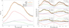 |
Fig. 1 Dust compositional fits to the N-band MATISSE data. Left panel: fit to the single-dish spectrum. Right panel: fits to the six correlated spectra. The solid yellow curve is the total model spectrum, while the green, red, and purple lines show the contributions from the individual disk zones. The thin blue line is the model stellar spectrum. |
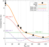 |
Fig. 2 Correlated flux density as function of the baseline length at a selected wavelength, 10 µm. The contributions of the three disk zones are the green, red, and purple lines, while the correlated flux curve of the whole disk is the orange solid line. Filled circles indicate the MATISSE N-band data points. The zero baseline data point is the single-dish flux. The thin blue line is the contribution of the central star. |
4.2 TGMdust runs
After the retrieval of the silicate composition with specfit, we run MCMC fits with our TGMdust code, using the full data-set covering the HKLMN bands. We fit the visibility data in the 1.6–12.3 µm wavelength range, and the SED between 1.25 and 18 µm. In these runs we fixed the relative mass fractions between the different silicate components, and the inner radii of the outer two zones. This is because those parameters are well constrained by the N-band only modeling with specfit. We choose to fit the inner radius of the disk, because that is better constrained with the shorter wavelength VLTI data (HKL bands). In addition to silicates, here we consider dust components responsible for the continuum opacity of the disk, namely iron and amorphous carbon. We attempt to determine their mass fractions, expecting that the featureless opacity curves of those species (Fig. D.3) might be better constrained using the wide wavelength span of the full data set. We perform two separate runs, one with silicates and iron, the other with silicates and carbon grains. We choose a population of two grain sizes, 0.1 µm and 2 µm, like in the case of the silicate grains. We have 15 fit parameters in total: the inner radius of the disk (R1), the temperature at the inner radius (Tin), the power law exponent of the temperature profile (q), the three surface densities at the zone inner edges (Σ0,i), the three surface density gradients (pi), and the mass fractions of either iron or carbon per grain size per zone (ci,small/large, six mass fractions).
Each MCMC run consists of 50000 steps with 32 walkers. When estimating the best-fit values, the first 20000 steps are discarded. For the χ2, we first calculate separately the χ2 values for the SED  and for the visibility data
  . In case of the SED the χ2 is calculated using the logarithms of the values, which helps to better fit the overall shape and flux levels of the SED. To equalize the weight of the visibilities in the fitting, we multiply
  by a factor of w = 3. This ensures a similarly good fit for both data types. With other values for w we found that either the SED fit or the visibility fit is much worse than the other. The total χ2, used in the optimization, is then
  , where NSED and NV are the number of fit data points in the SED and in the visibility data, respectively. The best-fit parameter values are chosen to correspond to the sample with the lowest
  in the chain, and the uncertainties of the parameters are taken as the 16–84 percentile ranges of the respective posterior distributions.
In Table 4, we list the best-fit parameters from both modeling runs, along with the fixed parameters and χ2 values. The results of the modeling with iron grains are presented in the following figures: Fig. 3 shows the model images at several wavelengths, Fig. 4 shows the radial surface brightness profiles, Fig. 5 shows the fit to the data, and Fig. 7 shows the vertical optical depth profiles. The corresponding figures for the model with carbon grains are Fig. G.2 (model images), Fig. G.3 (radial surface brightness profiles), Fig. 6 (fit to the data), and Fig. G.4 (vertical optical depth). The corner plots of the MCMC runs are presented in Fig. G.1 (run with iron) and Fig. G.5 (run with carbon). The model images were produced by interpolating Eq. (4) on a rectangular grid, also applying the inclination effect.
The iron and carbon runs provide similar fits to the data, with slightly better χ2 values for the run with iron (Table 4). Looking at the left panels in Figs. 5 and 6, the fits to the visibilities are nearly identical. The fit quality is generally good, especially in the N band, while at shorter wavelengths there are small to moderate systematic differences between the model and the data. For instance, the HKL data points at <30 Mλ spatial frequencies14 are systematically lower than the model points, indicating that at those wavelengths the disk is actually more extended than the model prediction. In contrast, in the M band, the data points exceed the model points, indicating that the disk emission in M band is slightly more compact than the model. These differences suggest that the disk has more substructure than what our 3-zone model can capture. Although the  values are close to each other, the model with iron can reproduce the SED much better than the model with carbon (right panels in Figs. 5 and 6).
The difference is most pronounced in the spectral region around the silicate feature, as the model with iron correctly fits both the silicate peak and the continuum level, while the model with carbon overestimates the continuum between 6 and 15 µm.
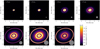 |
Fig. 3 Best-fit model images at various data wavelengths with the TGMdust run with iron grains. The brightness scaling is linear and homogeneous across all wavelengths. For a better perception of the fainter structural features, the images become saturated at 3.4 × 10⁻¹² W m−2 Hz−1 sr−1. The gray circles in the bottom left corner indicate the approximate beam size (estimated as 0.77λ/(Bp,max), where Bp,max is the maximum baseline length). |
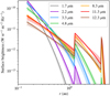 |
Fig. 4 Radial surface brightness profiles of the disk corresponding to the best-fit model with iron grains. The shaded area around each curve is the 16–84 percentile range from the last 5000 samples of the chain. |
Final results of the fits.
4.3 Disk structure
Both models yield very similar model images (Figs. 3 and G.2). There is a general trend that the emission gets more extended with increasing wavelength. In the H and K band, the flux comes almost exclusively from the innermost zone. From around 3 µm the second zone starts to appear, and in the N band emission all three zones contribute significantly. This is also reflected in the half-flux radius of the disk emission, listed in Table 4 for several wavelengths, that increases from 0.2 au at 2.2 µm to 2.3 au at 11.3 µm. The zone inner edges are sharply defined. The inner two zones are much brighter at 11.3 µm than at 8.3 or 12.5 µm; this is due to the increased emission of the silicate grains at that wavelength. The same can also be seen in the radial surface brightness profiles (Figs. 4 and G.3). The shaded areas in the surface brightness profiles, that reflect the uncertainty of the model fit, suggest that the profiles are quite well constrained by the data. We note that in the TGMdust run we do not fit the inner radii of the second and third zones, so the uncertainty of those parameters are not represented in the surface brightness profile plots. For the inner radius of the disk (R1 ≡ Rin), the TGMdust fit prefers a very small value <0.16 au, which differs significantly the value found in the specfit run  . Moreover, 0.16 au should be regarded as an upper limit, as the fit range had a lower boundary of 0.15 au, and the corner plots indicate that the fit would prefer even lower values. However, permitting a smaller inner radius would be unphysical, as the dust species in our model cannot exist at those regions because of the high temperatures there (> 1500 K). Consequently, the inner rim may have a distinct radial brightness profile or a special dust composition, or both, that our model cannot sufficiently reproduce.
Our models prefer a rather large brightness contrast at the inner edge of the third zone (~4 au), and a very steep decrease of the surface brightness outward. The edge at 4 au is well constrained by the N band data, however, the physical parameters of the third zone, such as the surface density profile and dust composition, are poorly constrained. This is because most of that radial zone is likely too cold to emit significantly in the N band. The emission of that zone mostly contributes at wavelengths longer than 20 µm, for that spectral region the model underestimates the SED. To conclude, our modeling can constrain the disk structure between ~0.15 and ~5 au.
4.4 Optical depth, temperature, and density profiles
The surface brightness profile (Eq. (4)) is constrained both by the SED (which sets the flux density) and by the VLTI data (which constrain the area from which we receive the flux). We assume that the source function is a blackbody, which is generally accepted for the radiation of circumstellar dust at IR wavelengths. The temperature profile is also well constrained by the simultaneous modeling of the SED and VLTI data, thanks to the wide spectral coverage of both data-sets. Thus, we argue that τ, the only remaining variable in Eq. (4), is robustly measured. Both Figs. 7 and G.4 indicate that the disk emission is not optically thick in the inner two zones (r < 4 au), as at λ > 3 µm τ remains below 0.4. Consequently, our assumption that the disk emission is optically thin, holds relatively well. The TGMdust model runs suggest an optically thick inner edge of the third zone, even in N band, while in the silicate compositional fits we generally assumed optically thin radiation. Thus, the specfit results for that zone are probably biased. At the same time, we have already noticed in Sect. 4.1 that the dust composition in the third zone is poorly constrained by specfit.
The temperature profile follows a relatively shallow decrease (q ≈ −0.5). The temperature at the inner edge is considerably higher than the generally assumed 1500 K (dust sublimation temperature), as it is ≈ 1800 K in the run with iron, and ≈ 1600 K in the run with carbon. There are several minerals which can endure such high temperatures. We discuss this subject further in Sect. 5.5.
The dust surface densities at the inner edges of the first two zones are in the range of 10−4−10−3 g cm−2. The iron-rich model gives a total dust mass of 5.7 × 10⁻⁵ MEarth in zone 1, and 2.6 × 10⁻⁴ MEarth in zone 2, while with the carbon-rich model we find 5.9 × 10⁻⁶ MEarth in zone 1 and 1.2 × 10⁻⁴ MEarth in zone 2. The model with carbon has a lower surface density and dust mass, compared to the model with iron. This is because the IR opacity of small carbon grains is roughly an order of magnitude above that of iron, so in order to produce the same amount of radiation less carbon is needed than iron, in terms of mass. Both TGMdust runs imply a very steep falloff of the surface density after 4 au. However, as was mentioned previously, our data cannot really constrain the disk parameters in the outer zone.
We note that in our modeling we consider only three, relatively small grain sizes (0.1, 2.0, and 5.0 µm), while it is very likely that the disk has considerable amount of larger (> 10 µm) grains which can hide a significant amount of mass because of their very low IR opacities. Thus, our derived masses may only reflect the mass present in small grains, and underestimate the total dust mass. A more general approach for this problem would be to apply a continuous grain size distribution (e.g., Mathis et al. 1977), but that is out of scope of the current study.
The models indicate that we need significant amounts of either iron or carbon in the dust mix in order to be able to reproduce the data. However, their radial distribution and grain size ratios cannot be well ascertained. This is primarily due to the featureless opacity curves of these dust types, that makes it difficult to identify the specific dust components in our spectro-interferometric data. Still, based on the fits to the SED (Sect. 4.2), we have a preference for the model with iron grains. Looking at the iron dust mass fractions (ci,small, ci,large) one by one, the large grains in the inner zone  , and the small grains in the middle zone
  are relatively well constrained, while for the other components either we have upper limits, or no constraints within the fit ranges at all. In case of the model run with carbon we find that only the small grains in the inner zone
  are constrained well.
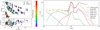 |
Fig. 5 Results of the TGMdust model run with iron grains. Left panel: fit to the visibilities with respect to the effective baseline length. The points are color coded for wavelength. The following wavelengths are plotted: 1.7 µm (PIONIER, gray), 2.2 µm (GRAVITY, purple), 3.3 µm (MATISSE L, blue), 4.75 µm (MATISSE M, green), 8.3 µm (orange), 11.3 µm (red), and 12.3 µm (brown, last three are MATISSE N data). Right panel: fit to the SED. The first three data points are 2MASS JHK measurements, the three points between 3 and 5 µm are extracted from our MATISSE LM-band data, and the points between 6 and 18 µm are taken from a Spitɀer observation, except the N band where the points are the average of the Spitɀer and our MATISSE single-dish spectra. |
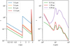 |
Fig. 7 Vertical optical depth of the best-fit disk model with iron grains. Left panel: Radial optical depth profiles at selected wavelengths. Right panel: Optical depth spectra at the inner edges of each zone. |
5 Discussion
5.1 Disk structure
Our results indicate a structured inner disk of HD 144432, with not less than three rings in the inner 5 au. This is a robust finding, as our multiband data set has a sufficient baseline sampling and resolution (0.2–1.4 au, depending on the wavelength) to recover those structures. As the closure phases of the VLTI data remain typically within ±10°, deviations from central symmetry are small, hence the observed structural features indeed should be concentric rings viewed slightly inclined. In our modeling the ring-like features arise as a result of a sudden increase of the radial surface brightness at the zone edges. In reality, the rings may have a rounded radial profile, but it is out of the scope of this study to constrain that aspect. Chen et al. (2016a) performed radiative transfer simulations to fit a set of H, K, and N band interferometric data on HD 144432. Their best model (coined DA0) features an inner disk between 0.2 and 0.3 au, which is optically thin at λ = 2 µm in the midplane in the radial direction; and an optically thick outer disk between 1.4 and 10 au. Their inner disk may be the same structure as our zone 1 (0.15– 1.3 au), while their outer disk coincides with our disk zones 2 and 3 (r > 1.3 au). As they only had a single-baseline N band interferometric observation with MIDI, that was not enough to detect the ring at 4 au.
Nature of the dust inner rim. We now investigate whether the inner radius of our model disk could be the dust sublimation radius. The following equation from Dullemond & Monnier (2010) describes the temperature – radius relation of the dust, assuming thermal equilibrium with the stellar radiation:
 (7)
(7)
where Tdust is the dust temperature, L* is the stellar luminosity, taken as 11.6 L⊙ from our stellar atmosphere fitting (Sect. 3), ϵ is the cooling factor, and σ is the Stefan-Boltzmann constant. For regular grains we can assume sublimation at Tdust ≈ 1500 K, the usual value found in the literature (e.g., Dullemond & Monnier 2010). Following Eq. (10) in Dullemond & Monnier (2010) we calculate the values of ϵ for the dust mixes in the inner zone. For the dust mix with carbon, we get ϵ = 0.23, and for the mix with iron ϵ = 0.47. With these values we estimate a sublimation radius of 0.24 au for the carbon-rich dust, and 0.17 au for the iron-rich dust. Thus, the preference for a relatively small inner radius (<0.16 au) by the TGMdust fit can be still consistent with the dust sublimation radius. However, the inner temperatures in our best fits are 100–200 K above 1500 K. We can use Eq. (7) to calculate the radius (Rdust) corresponding to our fit inner temperatures (Tin). For the model with carbon-rich dust we get 0.17 au, and for the model with iron-rich dust we get 0.15 au. These values are remarkably consistent with our values for the inner rim radius (Rin). Still, regular (sub-)µm-sized dust grains are not expected to survive at temperatures significantly above 1500 K. We note that the uniform sublimation temperature which we applied in our modeling oversimplifies the complex nature of various grain materials with significantly different evaporation temperatures (e.g., Gail 2004). We explore this issue further in Sect. 5.5. There is also a possibility that the disk structure and dust composition at the inner rim is more complicated than that our model can represent. For more accurate results on the physical conditions near the dust inner rim, one has to run proper radiative transfer models with scattering included, also accounting for the height and shape of the inner rim.
To put our results into context, Chen et al. (2012) calculated the radius of the K band emission from interferometric model fitting. The K band radiation is expected to come almost exclusively from the dust inner rim, so the K band disk size is a good proxy for the dust sublimation radius. Their value for the K band ring radius (0.17 au) is in agreement with our finding for the inner rim.
Two planet-induced gaps? One might ask whether the dark regions between the ring-like features are real disk gaps, or just shadowed regions. As in our modeling we do not represent the vertical extent of the disk, we cannot address this question. Chen et al. (2016a) explored this aspect in their RADMC-3D simulations with a puffed-up inner rim as the source of shadowing. They found that the self-shadowed model does not fit the data well, as it provides too low flux in the near-IR, and too much flux at 10–100 µm.
If the dark regions are indeed gaps, they might have been opened by massive planets residing in the disk (Asensio-Torres et al. 2021). It has been shown that the width and depth of disk gaps in the gas surface density profile are closely related to the planetary mass (Kanagawa et al. 2015). We assume that the µm-sized dust which we detect in our IR data is colocated with the gas, as expected for such small grains (e.g., Fouchet et al. 2010; Pohl et al. 2016). Here we use the Eq. (5) in Kanagawa et al. (2016) to estimate the masses of the putative gap-opening planets residing in the inner disk of HD 144432. The equation requires the gap width which is not straightforward to derive from our modeling, as we represent the surface brightness profile in each disk zone by a power law, and the dark gap-like regions in our images (Fig. 3) have just one well defined edge (the outer one). Here we assume that the surface density at the gap inner edge in zone 1 is equal to the surface density at the gap outer edge which coincides with the inner radius of zone 2. Thus, we get a gap inner edge at r ≈ 0.6 au, and an outer edge at 1.26 au. We place our planet in the middle position at Rp1 = 0.93 au. From the temperature profile in our best-fit model with iron grains we calculate the aspect ratio (H𝑔/Rp1 = 0.038, where Hg is the gas pressure scale height) of the disk at the location of the planet assuming hydrostatic equilibrium. For the stellar mass, we take 1.8 M⊙ (Guzmán-Díaz et al. 2021). The gap width is also influenced by the α viscosity parameter of the disk which is the source of considerable uncertainty. For a relatively low α value (10−4) we get a planet mass of 0.4 MJup, while for a higher value (α= 10−3) we get 1.3 MJup.
For the gap-like region in zone 2, we cannot define the gap inner edge as we did it in the first case, because the surface density at the outer edge of the second gap (i.e., the inner edge of zone 3) is much higher than the surface density anywhere in zone 2. Thus, for simplicity, we assume that the gap edges coincide with the inner (1.3 au) and outer (4.1 au) limits of zone 2. We place the planet in the middle of the zone at Rp2 = 2.7 au, where we estimate the aspect ratio to be Hg/Rp2 = 0.048. We get a planet mass of 1.3 MJup and 4.1 MJup for the low and high viscosity case (α = 10−4 and 10−3), respectively. Thus, we argue that both gap-like regions (one at ~0.9 au, the other at ~3 au) in the inner disk of HD 144432 might host gas giant planets, assuming that the structures we detect are tracing the overall density profile. In Fig. 8 we present a sketch of the disk of HD 144432, as we conceive it from our VLTI data and modeling, with the locations of the putative planets indicated.
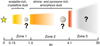 |
Fig. 8 Sketch of the disk of HD 144432, as seen by VLTI. We show the three ring-like structures, and the possible gaps between them. In the gaps we indicate two putative Jupiter mass planets. The cold outer disk, shown as a gray patch, cannot be constrained by our data. |
5.2 An optically thin inner disk
In physical models of optically thick planet-forming disks the surface layer, which is directly illuminated by the central star, gets superheated, while the deeper regions remain cold (e.g., Chiang & Goldreich 1997). In this case the warm to hot surface layer dominates the near-IR continuum and also gives rise to the dust spectral emission features, while the layer immediately below the superheated disk photosphere is expected to be significantly colder and to emit only at longer, mid-IR wavelengths. This requires a strong vertical temperature gradient in the disk, otherwise the thermal IR emission becomes partially optically thick, and the silicate spectral feature gets weaker. It is not straightforward to distinguish between this scenario and the case for a really optically thin disk. It might happen that the radiation we observe in HD 144432 comes from a superheated layer, mimicking an optically thin component. Still, the fact that we were able to reproduce both the level of the IR continuum emission and the silicate feature, using only one temperature gradient component per radial zone, is a strong indication for an optically thin emission.
Furthermore, Chen et al. (2016a) have already demonstrated in their RADMC-3D simulations that an optically thin inner component (between 0.2 and 0.3 au) is indeed compatible with the SED and IR interferometric data of HD 144432. For comparison, in our modeling we found evidence for optically thin IR emission coming from the inner two disk zones (<4 au, Sect. 4.4). We note that Chen et al. (2016a) reported the optical depth measured in the midplane in the radial direction (τ1(2 μm) = 0.14), that is not directly comparable to our τ, which is measured in the vertical direction. Thus, instead of the optical depths we opt to compare dust masses. They reported a dust mass for their inner disk component of 1.8 × 10⁻¹¹M⊙. Our dust mass estimations for the inner zone of our model (between 0.15 and 1.3 au) are 1.7 × 10⁻¹⁰M⊙ with the iron-rich dust mix, and 1.8 × 10⁻¹¹M⊙ with the carbon-rich dust. A word of caution here is that the dust mixes in these models may have significantly different opacities, so having similar dust masses does not guarantee that the optical depths are also similar. Still, as Chen et al. (2016a) used carbon grains in their modeling, it seems plausible that their opacities are similar to our carbon-rich model opacities. In that case their model is in remarkably good agreement with ours, in terms of total dust mass and optical depth. To further investigate the optical depth aspect, we would need proper radiative transfer modeling of our data set which is out of scope of this study.
As a final note, the reduced optical depth in the inner disk of HD 144432 might indicate that the disk is being depleted, emphasizing the transitory nature of this object. Massive planets may halt the inward radial drift of dust grains, trapping them in outer rings or vortices (Fedele et al. 2017). Alternatively, photoevaporative and magnetohydrodynamic disk winds can be also be responsible for the clearing of the inner disk (Pascucci & Sterzik 2009; Lesur et al. 2022).
5.3 Dust composition
Radial mineralogy gradients. An important result from our modeling is the confirmation of radial mineralogy gradients which were first observed by van Boekel et al. (2004). From an analysis of VLTI/MIDI N-band spectro-interferometric data they measured a crystallinity fraction of  in the 1–2 au disk region, and
  in the 2–20 au disk region. The radii of their disk regions were estimated from the baseline lengths of the observations. This method only gives a rough approximation, assuming that the interferometer collects the light from an aperture corresponding to the spatial resolution. In our modeling we were able to constrain the spatial extents of the disk zones with different mineralogical compositions much more precisely. In the specfit run, we found that the inner zone (0.2–1.3 au) has a crystallinity fraction of
  , while in the outer zones the same number is 20 ± 10%. These numbers match well with the values found by van Boekel et al. (2004) within the error bars, and also agree with our previous findings presented in Varga et al. (2018).
Alternatively, optically thick emission from the hot inner rim can also cause the inner disk spectra to show weaker silicate peaks, as shown by Meijer (2007). However, in our TGMdust fits we found that the IR radiation from the disk inner edge is optically thin (τ < 0.4). Thus, we do not see much support for a bright, optically thick inner rim in the disk of HD 144432 from our data.
Comparison with disk-integrated mid-IR spectroscopy. van Boekel et al. (2005) and later Juhász et al. (2010) performed dust compositional fits to N-band single-dish (TIMMI2 and Spit𝓏er) spectra of HD 144432. van Boekel et al. (2005) found a fit with 53% small (0.1 μm) amorphous olivine, 42% large (1.5 μm) amorphous pyroxene, and a small fraction of crystalline dust, mainly small forsterite (1.9%). Juhász et al. (2010)
in their fits to Spit𝓏er spectra between wavelengths 5 and 17 μm found that the main amorphous constituents are large (2 μm) amorphous olivine (42%), small (0.1 μm) amorphous pyroxene (19%), and large amorphous pyroxene (15%). Among the crystalline species, their fit preferred more enstatite (6.1%) than forsterite (2.3%). The results of these studies differ significantly, indicating that there is an inherent ambiguity in dust compositional fits to mid-IR silicate spectra. There are several contributing factors to this, like the selection of dust species to fit, the choice on the sizes of the grains, how the opacity curves are calculated (cf. Figs. 1 and 2 in Juhász et al. 2010), and the differences in the underlying disk model. Our silicate fit is not directly comparable to the aforementioned studies, because we dissected the disk into several zones, and obtained a composition for each zone. Still, our values in the disk zone 2 are comparable to the results by Juhász et al. (2010), as both feature a large contribution from large olivine and small pyroxene grains, and a preference for more enstatite than forsterite. Although our MATISSE N band spectro-interferometric data have lower S/N than the Spit𝓏er spectrum, we argue that our data have more constraining power in the compositional fits, because we have seven spectra (one single-dish and six correlated spectra) probing the same object.
5.4 Comparison with condensation sequences
The expected rich mineralogy of disks. While only a few dust species have been directly detected in the interstellar and circumstellar medium so far (mainly forsterite, enstatite, silicon carbide, and polycyclic aromatic hydrocarbons), there is evidence that the diversity of minerals in the cosmic dust is far richer. The evidence mainly comes from the analysis of Solar System interplanetary dust (IPD) grains, thought to be of presolar origin (e.g., MacKinnon & Rietmeijer 1987; Lodders & Amari 2005; Engrand et al. 2023). For example, carbon and iron are both found in the IPD and in meteorites (Anders 1964). Moreover, the planets in the inner Solar System are mostly composed of refractory elements: the main refractories Mg, Al, Si, Ca, Fe, Ni have a mass fraction of 67% in Earth, and 84% in Mercury (Morgan & Anders 1980). Most of these elements had been locked in the dust grains of the presolar nebula, before they got incorporated in planetary bodies. As many of the supposed materials in the cosmic dust have only weak or nonexistent optical-IR spectral features, the rich mineralogy of the interstellar and circumstellar dust mostly remains to be hidden from our observations.
Modeling condensation sequences with GGchem. Chemical modeling of dust condensation offers an alternative way to assess the variety of minerals which could exist under the physical conditions found in circumstellar disks. Here we investigate the expected diversity and distribution of solid state materials in a disk like HD 144432, using the thermo-chemical equilibrium code GGCHEM (Woitke et al. 2018). GGCHEM calculates the chemical composition of astrophysical gases, with the option to include the formation of condensates. We aim to address the following questions with GGCHEM:
The radial distribution of forsterite (Mg2SiO4) and enstatite (MgSiO3)15.
The nature of dust species which can exist in the innermost disk regions where T > 1500 K.
The amount of carbon and iron which condensates to dust grains in the disk.
For the input gas composition, we use the stellar abundances of C, O, Fe, Mg, Si reported by Kama et al. (2015) for HD 144432. For the rest of the elements (H, He, N, Na, Al, Ca, Ti, S, Cl, K, Li, F, P, V, Cr, Mn, Ni, Zr, W), we use Solar abundances by Asplund et al. (2009). GGCHEM calculates the concentration of the end products as function of the temperature and gas pressure (or hydrogen density). We define a pressure-temperature profile (pgas – T) based on the minimum mass solar nebula description by Hayashi (1981), but for the T (r) and Σ (r) radial profiles we use the power law exponents found for zone 1 in our TGMdust run with iron grains. For the calculation of pgas, we used Eqs. (B.5)–(B.9) from Jorge et al. (2022), assuming that the disk is vertically isothermal. The results are shown in the top panel of Fig. 9, indicating that the most abundant condensates between 0.2 and 1 au are iron and forsterite. We see no enstatite forming at all, which is also found by Jorge et al. (2022) if the Mg/Si ratio is above the solar value by 0.17 dex. In the case of HD 144432, the Mg/Si ratio is even higher, 0.26 dex more than in the Sun.
We also performed a chemical calculation with Solar abundances taken from Asplund et al. (2009), shown in the bottom panel of Fig. 9. The plot indicates that both forsterite and enstatite form in a solar-like gas mixture, that is consistent with the results of our silicate compositional fits for HD 144432. The figure also shows that the radial distribution of the two main silicate minerals are different: while enstatite can be found between 0.3 and 2 au, forsterite has a broader distribution from 0.2 au to 5 au and beyond. In our results we do not find evidence for such radial distribution, as our model fit requires significant amounts of enstatite in all three disk zones. Finally, we note that our estimation (0.08 dex) for the Mg/Si ratio of the disk (Sect. 4.1) is very close to the solar value (0.09 dex).
The problem of enstatite. N band spectroscopic and spectro-interferometric data clearly indicate that there is significant amount of enstatite in the disk around HD 144432, in stark contrast with the prediction of our GGCHEM calculation with the stellar abundances of HD 144432. We consider two scenarios to resolve this discrepancy: either the equilibrium condensation conditions do not hold in the disk, or the chemical composition of the disk differs from that of the stellar photosphere. The general notion is that the host star abundances are good proxies for the chemical composition of the cloud from which both the star and the disk are formed (Adibekyan et al. 2021). However, Kama et al. (2015) found that stars hosting group I disks, known to have large gaps, are depleted in Fe, Mg, and Si, compared to the Sun and to stars hosting group II (flat, continuous) disks. They suggested that this depletion is caused by giant planets which block the accretion of dust onto the star, while not affecting gas accretion. The same planets can also open gaps in the disk, making it exhibiting a group I type SED. Although HD 144432 has a group II disk, Kama et al. (2015) detected a depletion of refractory elements similar to the stars hosting group I disks. Thus, it seems plausible that the disk of HD 144432 has a solar-like elemental chemical composition, and the depletion of the stellar photosphere in Fe and Si is caused by a giant planet in the inner disk (<5 au) halting the radial drift of the dust. The planet, which might be responsible for the inner disk substructure as well, could be located in one of the gap-like regions between two rings (either at ~ 1 or at ~3 au). However, there are two problems with this idea: i) small (sub-)μm-sized dust grains are relatively well coupled to the gas, and ii) we detect enstatite even in the inner zone (0.2–1 au), where we do not expect a planet blocking the accretion at the inner edge.
Alternatively, the physico-chemical conditions in disks might be more complex than that we can represent with a simple disk model with equilibrium chemistry. GGCHEM calculates the gas and dust composition at every distance (temperature) by minimizing the Gibbs free energy. However, the dust will have seen a complex history of growth, settling and mixing, which is not accounted for in an equilibrium calculation. For instance, Gail (2004) concluded that by taking into account radial mixing, the bulk of the grains at temperatures lower than ~ 1000 K should be enstatite. This is because all forsterite grains, which move from the innermost regions outward, pass through a region in which they are converted to enstatite, and at further out these reactions could freeze out, so that conversion back to forsterite would not take place. Furthermore, equilibrium theory cannot well describe the complex nucleation processes of solids, and phase-equilibrium models have no history. As illustrated in Fig. 11 of Herbort et al. (2020), condensation of μm-sized grains is intrinsically fast (<1 s), but the timescale of annealing is much longer (on the order of 1 Myr at T = 900 K). Therefore, if the disk has a constant temperature structure, and the dust is at rest, only the innermost part can provide conditions for phase-equilibrium. Pignatale et al. (2016) demonstrated that equilibrium condensation can be a valid assumption for the disk region where T ≳ 600 K (r ≲ 1 au in our model).
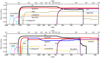 |
Fig. 9 Concentration of various condensates (normalized to hydrogen atom number density) as a function of radius and temperature from our calculation using the thermo-chemical equilibrium code GGCHEM (Woitke et al. 2018). Top: plot showing the concentration using the photospheric elemental abundances of HD 144432. Bottom: plot showing the concentration using Solar elemental abundances. For clarity, we show a selection of the condensates: we plot only those species which are among the top three most abundant condensates for at least one temperature value. The T (r) relation follows our best-fit TGMdust model with iron grains. The gas pressure-temperature profile follows a power law with p = 3.16 × 10⁻² bar at the maximum temperature T = 2000 K, and p = 1.79 × 10⁻⁶ bar at the minimum temperature T = 277.5 K. |
5.5 Hot dust at the inner rim
In Sect. 4.4, we noted that our models prefer a temperature at the inner rim that is 100–200 K above the sublimation temperature (~1500 K) of regular dust grains. From the GGCHEM calculation we can evaluate what kind of minerals can endure such high temperatures. Calculations with solar and with the HD 144432 abundances show similar results. The first two condensates forming are tungsten at ~2000 K, and zirconium dioxide (ZrO2) at ~1900 K, but they are not shown in our plots because of their very low concentrations (log10 (nsolid/n〈H〉) < −9.4). At slightly lower temperatures (~1850 K) corundum (Al2O3) forms, followed by perovskite (CaTiO3, not shown because its low abundance) and gehlenite (Ca2Al2SiO7) condensing at ~1700 K. This condensation sequence is very similar to what was found by Woitke et al. (2018) at pgas = 1 bar; the only difference is that in our calculation the condensation occurs at lower temperatures due to the lower pressures in our disk model.
The most abundant condensates (corundum and gehlenite) present at T > 1500 K have concentrations (~−6) about 30 times less than the major solid state species iron and forsterite. Moreover, the near-IR opacity of corundum (~100 cm2 g−1) is much lower than that of iron (~2000 cm2 g−1). Considering the difference in temperature and in the surface area, we estimate that the 3 μm flux from corundum grains at T = 1800 K located at 0.15 au is only 0.3% of the flux emitted by iron grains at T = 1500 K at 0.2 au radius. It remains to be determined, whether that apparently weak signal from corundum and other refractory grains could be detected in observational data.
5.6 Iron vs. carbon
A favored iron-rich composition. Condensation of carbon does not occur in the warm disk regions (r < 5 au, T > 300 K) if the gas has a solar C/O ratio (C/O = 0.55) or less. According to Kama et al. (2015), HD 144432 has a C/O ratio of 0.24. If we artificially increase the C/O ratio to ~0.9, we start to see graphite forming near a temperature of T = 1000 K. If C/O reaches 1, graphite becomes a major constituent in the dust mix between 850 K and 1250 K, corresponding to the radial region between 0.3 and 0.6 au. Such high C/O ratio seems to be unlikely in the majority of stars in our Solar neighborhood. In the Hypatia Catalog by Hinkel et al. (2014), which is a compilation of stellar abundance data within 150 pc of the Sun, only 2% of the stars have C/O > 0.9. Assuming a similar C/O distribution for the nearby star forming regions and YSOs, we suggest that in the warm inner disk regions (r < 5 au) of planet-forming disks most, if not all, carbon is in the gas phase, while iron and iron sulfide (FeS, troilite) grains are major constituents of the solid mixture, along with forsterite and enstatite. Thus, small (sub-)μm sized iron grains should be the main source of dust continuum radiation at thermal IR wavelengths in disks. This is in line with the conclusions of Matter et al. (2020) who suggested to replace carbon with iron when modeling inner disk spectra of YSOs. For more discussion on the effects of varying C/O in inner disks, we refer to Matter et al. (2020).
Carbon in solid form is expected to be abundant in the cold outer disk, locked up in ices or as pre-stellar grains. Radial drift can cause that material to reach the inner disk. As a result, the inner disk would be populated by a mix of grains which had experienced chemical equilibrium conditions and grains which came from the outer disk, which is a scenario that cannot be ruled out for HD 144432. Indeed, the fact that we detect both crystalline and amorphous silicate grains may already signify that such a mix exists. Still, the inner Solar System planets are highly depleted in carbon, so there should be processes resulting in carbon-depleted inner disk solid reservoirs (Öberg et al. 2011). Klarmann et al. (2018) investigated the efficiency of oxidation and photolysis in the removal of carbon grains from the solid phase, and they found that radial transport of dust can easily prevent the depletion of carbon. They conclude that more efficient carbon-depletion mechanisms along with radial drift barriers are needed to prevent the replenishment of carbon in the inner disk. In a carbon-enriched environment, we can expect the presence of various hydrogenated carbon compounds which show spectral features in the mid-IR (Jones et al. 2017). In HD 144432, those carbonaceous features are much weaker than the silicate emission bands (Seok & Li 2017). Further observations by MATISSE using the medium spectral resolution mode (R ≈ 500) in L band may shed light on the spatial distribution of the carbonaceous dust in the disk of HD 144432. As far as iron is concerned, iron-rich grains should be present both in the population of grains which are produced by recondensation in situ, as well as from the outer disk, drifting inward.
In our modelling, we found evidence for a high abundance of enstatite in the disk of HD 144432. The combination of enstatite with iron is reminiscent of enstatite chondrites which are believed to be a major building block of the Earth and other inner Solar System bodies (e.g., Javoy 1995; Javoy et al. 2010).
By deriving elemental abundances from the dust composition that we fit (Tables 3 and 4), we can investigate what kind of rocky planets could form in the inner disk of HD 144432. In Table 5 we show our abundance values for HD 144432, compared with elemental abundances of Mercury, Earth, and CI chondrites. We selected the second disk zone (1.3 < r < 4.1 au) for the comparison, as that zone covers large part of the terrestrial planet forming region. The table shows that our model with iron-rich dust represents an elemental composition intermediate between that of Mercury and Earth. In contrast, the elemental composition of our model with carbon-rich dust has some similarities with the abundances of CI chondrites, although the correspondence is not particularly good. We note that in our models either we have iron but no carbon, or the other way around. With that we cannot account well for the composition of CI chondrites, as they contain significant amounts from both carbon and iron.
Carbon content and planet habitability. To put the iron vs. carbon dichotomy in a wider context, Hakim et al. (2019) has shown that exoplanets forming from carbon-enriched material will have, after differentiation, a graphite outer layer. Such a shell has major effects on the thermal evolution and geochemistry of the planet. Moreover, if the graphite layer is thick enough, it might prevent the silicate-rich mantle material to come to the surface. In this case the planet surface would be devoid of essential life-bearing elements (except of course carbon), making the planet potentially uninhabitable.
Chemical sorting by grain growth. Johansen & Dorn (2022) explored the grain growth of condensates forming in a gas of solar composition. They found that iron preferentially grows into sparser, bigger pebbles, while enstatite, forming at the same location, has smaller grain sizes. Consequently, the population of large iron grains becomes chemically separated from the silicate grains having Stokes numbers 10 times lower. They further propose that under such conditions streaming instability leads to the formation of iron-rich planets. They conclude that this formation mechanism can explain why Mercury is so enriched in iron, without the need for experiencing giant, mantle-stripping impacts. This study demonstrated both the crucial role of iron in the formation of terrestrial planets, and the importance of microphysics when dealing with dust evolution.
To conclude, our observations and modeling of HD 144432 show tentative evidence for the presence of iron in its planet-forming disk. This claim is partly based on the notion that our model with iron-rich dust provides a better fit to the SED, compared to our other model with carbon-rich dust. Furthermore, our chemical calculations in a disk model representing the pressure-temperature conditions in the HD 144432 disk also give support for an iron-rich chemistry, in agreement with numerous literature sources.
Comparison of elemental abundances between Mercury, Earth, CI chondrites, and our best-fit disk models for HD 144432.
6 Summary
In this paper, we studied the planet-forming disk around HD 144432 by modeling an extensive set of photometric and spectro-interferometric data covering the thermal IR wavelengths. Our data set includes new observations with VLTI/GRAVITY (K band) and VLTI/MATISSE (L, M, and N bands), and archival data from VLTI/PIONIER (H band). We introduced a new disk model, TGMdust, to image the inter-ferometric data, and to constrain the disk structure and dust composition. TGMdust can represent disk geometries without (single zone) or with substructure. In the latter case the disk is divided into multiple radial zones, each having its own surface density profile and dust composition. Our main results are as follows:
- 1
The disk within <5 au is structured. We need at least 3 zones to fit the data. Our best-fit model features an inner zone between 0.15 and 1.3 au, a second zone between 1.3 and 4.1 au, and an outer zone starting at 4.1 au. Each zone has a bright inner edge, thus the disk appears to show a three-ringed structure.
- 2
From our silicate compositional fits we find that the dust composition of the zones significantly differ from each other, indicating radial mineralogy gradients. Specifically, the mass fraction16 of crystalline silicates is about 61% in the innermost zone (<1.3 au), while only ~20% in the outer two zones.
- 3
By inspecting the fits to the MATISSE N band data, we find that the silicate spectral feature mostly originates from the second disk zone (1.3–4.1 au). We show that the silicate spectral feature in the correlated spectra is mixed with strong spatial modulation signatures, an effect caused by the ringlike substructures. We also find that the disappearance of the silicate feature in the longest baseline (Bp = 129 m) correlated spectrum is mostly due to spatial modulation effects, not to mineralogy gradients or radiative transfer effects, as was previously thought. As a general note, interpreting correlated spectra as proper spectra should be generally avoided, instead, interferometric modeling or image reconstruction should be applied.
- 4
To identify the dust component responsible for the infrared continuum emission, we explore two cases for the dust composition, one with a silicate+iron, the other with a silicate+carbon mixture. We can fit the interferometric data with both compositions equally well, however, the iron-rich model provides a better fit to the SED.
- 5
We find that the radiation from the inner two disk zones (r < 4 au) is mostly optically thin, having τ < 0.4 at wavelengths longer than 3 μm. This finding is consistent with the radiative transfer modeling results of Chen et al. (2016a).
- 6
Assuming that the dark regions in the disk are gaps opened by planets, we estimated the masses of the putative planetary bodies responsible for those structures. We find that both gaps, the one in zone 1 at ~0.9 au and the other in zone 2 at ~3 au, might be carved by approximately Jupiter mass planets.
- 7
In order to assess the hidden diversity of minerals in a planet-forming disk like HD 144432, we performed chemical equilibrium calculations of dust condensation with GGCHEM. Using solar elemental abundances in the GGCHEM calculation results in a dust mixture with major constituents iron, forsterite, and enstatite, in agreement with our modeling with the iron+silicate dust mix.
- 8
GGCHEM predicts the existence of some refractory minerals which can survive in the 1500–2000 K temperature range. The most abundant species under those conditions are corundum (Al2O3) forming at ~1850 K, and gehlen-ite (Ca2Al2SiO7) condensing at ~1700 K. We estimate that the 3 μm flux emitted by corundum grains at T = 1800 K located at 0.15 au is only 0.3% of the flux emitted by iron grains at T = 1500 K located at 0.2 au radius. It is still unclear whether that weak emission could be detected with current observational techniques.
- 9
Our GGCHEM calculations show that condensation of carbon does not occur in the warm disk regions (r < 5 au, T > 300 K) if the gas has a C/O ratio ≲ 0.9. We propose that in the warm inner regions (r < 5 au) of typical planet-forming disks most if not all carbon is in the gas phase, while iron and iron sulfide (FeS, troilite) grains are major constituents of the solid mixture, along with forsterite and enstatite. Thus, small (sub-)μm sized iron grains should be the main source of dust continuum radiation at thermal IR wavelengths in disks. We repeat the recommendation of Matter et al. (2020) who suggested to replace carbon with iron when modeling inner disk spectra of YSOs.
Our analysis exemplifies the need for detailed studies of the dust in inner disks with multiwavelength high angular resolution techniques. Currently, MATISSE is the only instrument which can resolve disks on au-scales in the N band, probing the warm, forsterite and enstatite rich dust, while at longer wavelengths JWST/MIRI may give insights to the cold dust population, ices, and gas chemistry (Kóspál et al. 2023; Grant et al. 2023; Perotti et al. 2023). Additionally, ALMA could possibly detect larger scale substructures like the r ≈ 4 au ring of HD 144432 at its highest spatial resolution. As of mid-2023, there is no high-resolution measurement of our target in the ALMA archive, only a measurement with the 7 m array, but that has a low spatial resolution of only 4.5″. In the coming years, more results on the mineralogy of planetary building blocks will be expected from the MATISSE GTO survey of YSOs.
Acknowledgements
MATISSE was designed, funded and built in close collaboration with ESO, by a consortium composed of institutes in France (J.-L. Lagrange Laboratory – INSU-CNRS – Côte d’Azur Observatory – University of Côte d’Azur), Germany (MPIA, MPIfR and University of Kiel), The Netherlands (NOVA and University of Leiden), and Austria (University of Vienna). The Konkoly Observatory and Cologne University have also provided some support in the manufacture of the instrument. GRAVITY has been developed in a collaboration by the Max Planck Institute for Extraterrestrial Physics, LESIA of Paris Observatory-PSL/CNRS/Sorbonne Université/Université Paris-Cité and IPAG of Université Grenoble Alpes/CNRS, the Max Planck Institute for Astronomy, the University of Cologne, the Centro Multidisciplinar de Astrofisica Lisbon and Porto, and the European Southern Observatory. Based on observations collected at the European Southern Observatory under ESO programmes 190.C-0963(D), 190.C-0963(E), 190.C-0963(F), 0100.C-0278(E), 0103.D-0153(C), 0103.C-0347(C), 0103.D-0153(G), 108.225V.003, 108.225V.011, and 108.225V.006. P. Ábrahám, F. Lykou and J. Varga are funded from the Hungarian NKFIH OTKA project no. K-132406. á. Kóspál, J. Varga, P. Ábrahám, F. Lykou, and F. Cruz-Sáenz de Miera have received funding from the European Research Council (ERC) under the European Union’s Horizon 2020 research and innovation programme undergrant agreement No 716155 (SACCRED). The research of J. Varga and M. Hogerheijde is supported by NOVA, the Netherlands Research School for Astronomy. J. Varga acknowledges support from the Fizeau exchange visitors program. The research
leading to these results has received funding from the European Union’s Horizon 2020 research and innovation programme under Grant Agreement 101004719 (ORP). F. Cruz-Sáenz de Miera received financial support from the European Research Council (ERC) under the European Union’s Horizon 2020 research and innovation programme (ERC Starting Grant “Chemtrip”, grant agreement no. 949278). P. Woitke acknowledges funding from the European Union H2020-MSCA-ITN-2019 under Grant Agreement no. 860470 (CHAMELEON). N. Morujão acknowledges the financial support provided by FCT/Portugal through grants PTDC/FIS-AST/7002/2020 and UIDB/00099/2020. This research has made use of the services of the ESO Science Archive Facility. This research has made use of the VizieR catalog access tool, CDS, Strasbourg, France (DOI: https://doi.org/10.26093/cds/vizier). The original description of the VizieR service was published in Ochsenbein et al. (2000). This research has made use of the Jean-Marie Mariotti Center OiDB service available at http://oidb.jmmc.fr. This work has made use of data from the European Space Agency (ESA) mission Gaia (https://www.cosmos.esa.int/gaia), processed by the Gaia Data Processing and Analysis Consortium (DPAC, https://www.cosmos.esa.int/web/gaia/dpac/consortium). Funding for the DPAC has been provided by national institutions, in particular the institutions participating in the Gaia Multilateral Agreement. This study has made use of the GGCHEM code, available at https://github.com/pw31/GGchem.
Appendix A VLTI data plots
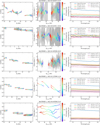 |
Fig. A.1 Calibrated MATISSE L band data sets. Left column: visibility as a function of the spatial frequency. Middle column: Closure phase as a function of the spatial frequency corresponding to the longest baselines of the triangles. Right panel: Correlated flux as a function of the wavelength. We also plot the single-dish spectrum, as the zero-baseline correlated spectrum. |
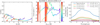 |
Fig. A.3 Same as Fig. A.1, but for the MATISSE N band data. We note that, as of DRS version 1.5.8, the sign convention of the N band phases are flipped with respect to the LM band phases (see also Gámez Rosas et al. 2022). This causes a 180° rotation of the N band images. This issue is no concern for us, as we do not use the N band closure phases in our modeling. |
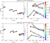 |
Fig. A.4 Calibrated GRAVITY data sets. Left column: visibility as a function of the spatial frequency. Right column: Closure phase as a function of the spatial frequency corresponding to the longest baselines of the triangles. |
Appendix B Additional notes on the MATISSE data processing
While the L band sensitivity of the instrument is more than enough to record good quality data on HD 144432 using the ATs, it is not the case in N band where only the UT data can be used. For obtaining correlated fluxes we apply the so-called coherent processing provided by the DRS pipeline, while the visibilities are processed using the incoherent method. The coherent algorithm has a gain in S/N compared to the incoherent method. Due to this advantage, coherently processed correlated fluxes are especially useful in the N band. For the specfit modeling, we directly used those data. However, the PIONIER and GRAVITY data does not contain correlated flux, only visibilities, thus for a homogeneous modeling of all VLTI data sets we need to use visibilities even in the N band. We opt not to use the incoherently processed N band visibilities, because of their lower quality. Instead we apply a special treatment to the N band correlated fluxes by dividing them with the average single-dish flux, in this way producing coherently processed visibility data. We use these specially calibrated N band visibilities in the TGMdust runs.
The L and M band MATISSE data comes in two flavors: chopped and non-chopped. Chopping helps to suppress the sky background, which gets increasingly dominant in the M band. Thus, in M band it is mandatory to use chopped data, while in L band both chopped and non-chopped data may be used. During chopping the frequent switching between the object and sky positions might cause to lose track of the adaptive optics guiding or the fringe tracking, which results in bad quality data. Thus, when both non-chopped and chopped L band data-sets were available, we carefully inspected both products, and selected the one which we deemed more reliable (the one with smaller error bars).
Appendix C Visibility calculation
The visibility function is the Fourier-transform of the object’s image on the sky. IR interferometers sample the visibility function at distinct spatial frequencies, set by the baseline length between the telescope pairs. The visibility function is a complex quantity, and in IR interferometry it is usually represented by its absolute value and phase. The absolute value of the visibility can be expressed either as a unitless quantity, or in flux units. In the latter case it is known as the correlated flux. It is the correlated flux which is directly measured by the interferometer. In polar coordinates the Fourier-transform becomes the Hankel-transform. For an object with circular symmetry, the correlated flux can be expressed from the radial surface brightness profile (Iv (r)) as follows:
 (C.1)
(C.1)
where Bp is the projected baseline length, J0 is the Bessel function of the first kind of order zero, and Rin, Rout are the inner and outer radii of the object, respectively. The Bp/λ is the spatial frequency. The argument of J0 is in radians. In our multi-zone disk model, Fcorr,v,i·is the correlated flux of the i-th zone, with the integration limits being the zone boundaries Rin = Ri and Rout = Ri+1. The formula above assumes a circularly symmetric object image. If the image is elliptic, such as an inclined thin disk, the visibility function also depends on the position angle of the baselines (θB), not just on their lengths. In that case we can transform the projected baseline lengths so that we remove the effect of the inclination:
 (C.2)
(C.2)
where ∆θ = θB − θ is the difference between the position angle of the baseline and the position angle of the major axis of the object image (θ). Using Beff removes the θB dependence in the visibility calculation, and we can apply Eq. C.1, as if the object image were circular.
In our model the central star is represented as a point source, thus its correlated flux equals its (single-dish) flux. The correlated fluxes of the disk radial zones (Fcorr,v,i), and that of the central star (Fv,Star) are simply added together:
 (C.3)
(C.3)
Finally, we calculate the unitless visibility (Vv), by normalizing the correlated flux with the single-dish flux (Fv):
 (C.4)
(C.4)
Appendix D Opacity curves
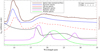 |
Fig. D.1 7–35 µm opacity curves of pyroxene, olivine, and various iron oxides, compared with the normalized Spitzer spectrum of HD 144432 (brown curve, AOR: 3587072). The Spitzer spectrum was normalized by dividing the data with the source function of our best-fit model. Optical constants of iron oxides were downloaded from the Jena Database of Optical Constants for Cosmic Dust (https://www.astro.uni-jena.de/Laboratory/OCDB/mgfeoxides.html). The original source for wüstite is Henning et al. (1995). Optical data for hematite and magnetite come from Amaury H.M.J. Triaud (unpublished). The opacity curves were generated with optool, using the distribution of hollow spheres (DHS) scattering theory. The upper boundary of the hollow sphere distribution (ƒmaχ) is 0.7. All curves are arbitrarily scaled and shifted to aid visual comparison. |
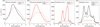 |
Fig. D.2 N band opacity curves of the silicate minerals used in this work. Red color indicates the subset used in the final dust modeling. |
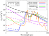 |
Fig. D.3 Opacity curves in the full wavelength range of the data. Shown only the subset used in the final dust modeling, including iron and carbon as well. |
Appendix E Two-step optimization procedure
Our approach for finding the best-fit model is detailed in the following. First, we constrain the silicate composition and the main structural disk parameters by fitting only the N band MATISSE data (six correlated spectra and the single-dish spectrum between 8 and 13 µm). For this purpose we use our own idl software, based on the specfit dust compositional fitting tool by Juhász et al. (2009). In our code we implemented our multi-zone temperature gradient model, and added the functionality to model interferometric data, while we retained the original fitting procedure of specfit. The optimization of the disk structural parameters is done by a genetic optimization algorithm named pikaia (Charbonneau 1995). In each optimization step of the genetic algorithm, a spectral decomposition is employed by a bound constrained linear least-squares fitting algorithm (Lawson & Hanson 1974), in order to evaluate the dust mass fractions. The latter step requires a change in our model when calculating the surface brightness profile in Eq. 4:
 (E.1)
(E.1)
Here we assume the disk to be optically thin (τ ≪ 1) at our observing wavelengths. Thus, we can calculate the total emission by simple linear addition of the contributions from the individual dust components. This is needed by the spectral decomposition algorithm in the specfit code. The final result of this modeling is the set of fit structural parameters and dust mass fractions.
We expect that the N-band data alone cannot differentiate between the dust species with featureless opacity curves (iron and carbon). This is because the opacities of those species look very similar in that spectral region. Thus, we do not include either carbon or iron in our specfit runs. Instead we include a hidden dust component with a power law opacity curve to represent the dust responsible for the featureless continuum. The exponent of the power law is a fit parameter, while we fix the opacity17 at 8 µm at 500 cm2/g.
In the second modeling step we aim to constrain the disk structure overall. The fitting procedure employed in the first step is very capable at constraining the dust composition, but it can only model optically thin emission. The linear spectral decomposition gives erroneous results if in some spectral regions the emission is optically thick. The latter constrain motivated our choice to restrict the fitting with specfit to the N band. To overcome that limitation, we apply our own model fitting tool, TGMdust18 (Temperature Gradient Modeling with dust), which is a python implementation of our multi-zone disk model described in Sect. 3. For the optimization we use emcee, an MCMC ensemble sampler (Foreman-Mackey et al. 2013a,b). In TGMdust we use our original assumption for the radiative transfer, described in Eq. 4, capable to represent optically thick emission. We note that the linear combination assumption employed in the previous step provides nearly equivalent results to the TGMdust fits if the dust emission is optically thin. In this step of modeling, we use all data we have, not just the N band. The large number of model parameters (44 in the case of the 3-zone model) might prevent the MCMC sampler from reaching convergence. Thus, with TGMdust we fit a limited set of parameters, and we use the dustmass fractions obtained in the first step by specfit as fixed parameters.
Appendix F Degeneracy in the spectral decomposition
As was shown by van Boekel et al. (2005) (see Sect. 5.2 and Fig. 8 therein), the silicate spectral templates used in the spectral decomposition are degenerate to a degree. We investigated this issue in our specfit model run by inspecting the individual samples. We found several good-fitting solutions with a dust composition differing considerably from the best fit. One example is shown in Table F.1, and in Figures F.1, F.2. The χ2 of the alternative solution is 1.7 times larger than that of the best fit. The fit is qualitatively similar to that of the best fit, except at the edges of the band (<8.5 μm and > 12.5 μm) where there is a larger deviation from the data. The zone boundaries (0.2, 0.9, and 4.0 au) are close to the values of the best fit, while the mass fraction values indicate degeneracies between large pyroxene and enstatite in zone 2, and between large olivine, small pyroxene, and enstatite in zone 3. These findings imply that despite the degeneracies in the silicate spectral templates, the disk substructrures (zone boundaries) are robustly constrained by our modeling.
An example for an alternative good-fitting solution for the silicate spectral decomposition. The abundances are given as fractions of the total dust mass in percent, excluding the hidden dust component responsible for the continuum emission.
 |
Fig. F.1 Same as Fig. 1, but for a specfit solution corresponding to the dust mass fractions listed in Table F.1. |
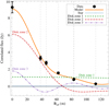 |
Fig. F.2 Same as Fig. 2, but for a specfit solution corresponding to the dust mass fractions listed in Table F.1. |
Appendix G Supplementary model plots
G.1 TGMdust model run with iron grains
 |
Fig. G.1 Corner plot showing the posterior distributions of the MCMC samples from the run with iron grains. We note that in case of the surface densities and mass fractions we fit the logarithm of the quantities. |
G.1 TGNdust model run with carbon grains
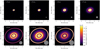 |
Fig. G.2 Best-fit model images at various data wavelengths with the TGMdust run with carbon grains. The brightness scaling is linear and homogeneous across all wavelengths. For a better perception of the fainter structural features, the images become saturated at 3.4 × 10⁻¹² W m−2 Hz−1 sr−1. The gray circles in the bottom left corner indicate the approximate beam size (estimated as 0.77λ/(Bp,max), where Bp,max is the maximum baseline length). |
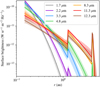 |
Fig. G.3 Radial surface brightness profiles of the disk corresponding to the best-fit TGMdust model with carbon grains. The shaded area around each curve is the 16–84 percentile range from the last 5000 samples of the chain. |
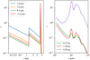 |
Fig. G.4 Vertical optical depth of the best-fit disk model with carbon grains. Left panel: Radial optical depth profiles at selected wavelengths. Right panel: Optical depth spectra at the inner edges of each zone. |
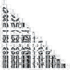 |
Fig. G.5 Corner plot showing the posterior distributions of the MCMC samples from the run with carbon grains. We note that in case of the surface densities and mass fractions we fit the logarithm of the quantities. |
References
- Ábrahám, P., Juhász, A., Dullemond, C. P., et al. 2009, Nature, 459, 224 [Google Scholar]
- Adibekyan, V., Dorn, C., Sousa, S. G., et al. 2021, Science, 374, 330 [NASA ADS] [CrossRef] [Google Scholar]
- ALMA Partnership (Brogan, C. L., et al.) 2015, ApJ, 808, L3 [Google Scholar]
- Anders, E. 1964, Space Sci. Rev., 3, 583 [NASA ADS] [CrossRef] [Google Scholar]
- Andrews, S. M., Huang, J., Pérez, L. M., et al. 2018, ApJ, 869, L41 [NASA ADS] [CrossRef] [Google Scholar]
- Asensio-Torres, R., Henning, T., Cantalloube, F., et al. 2021, A&A, 652, A101 [NASA ADS] [CrossRef] [EDP Sciences] [Google Scholar]
- Asplund, M., Grevesse, N., Sauval, A. J., & Scott, P. 2009, ARA&A, 47, 481 [NASA ADS] [CrossRef] [Google Scholar]
- Avenhaus, H., Quanz, S. P., Garufi, A., et al. 2018, ApJ, 863, 44 [NASA ADS] [CrossRef] [Google Scholar]
- Bailer-Jones, C. A. L., Rybizki, J., Fouesneau, M., Demleitner, M., & Andrae, R. 2021, AJ, 161, 147 [Google Scholar]
- Boccaletti, A., Di Folco, E., Pantin, E., et al. 2020, A&A, 637, A5 [NASA ADS] [CrossRef] [EDP Sciences] [Google Scholar]
- Bouwman, J., Meeus, G., de Koter, A., et al. 2001, A&A, 375, 950 [NASA ADS] [CrossRef] [EDP Sciences] [Google Scholar]
- Charbonneau, P. 1995, ApJS, 101, 309 [Google Scholar]
- Chen, L., Kreplin, A., Wang, Y., et al. 2012, A&A, 541, A104 [NASA ADS] [CrossRef] [EDP Sciences] [Google Scholar]
- Chen, L., Kreplin, A., Weigelt, G., et al. 2016a, A&A, 586, A54 [NASA ADS] [CrossRef] [EDP Sciences] [Google Scholar]
- Chen, P. S., Shan, H. G., & Zhang, P. 2016b, New Astron., 44, 1 [Google Scholar]
- Chiang, E. I., & Goldreich, P. 1997, ApJ, 490, 368 [Google Scholar]
- Cutri, R. M., Skrutskie, M. F., van Dyk, S., et al. 2003, VizieR Online Data Catalog: II/246 [Google Scholar]
- Desch, S. J., & Cuzzi, J. N. 2000, Icarus, 143, 87 [Google Scholar]
- Dominik, C., Min, M., & Tazaki, R. 2021, Astrophysics Source Code Library [record ascl:2104.010] [Google Scholar]
- Dorschner, J., Begemann, B., Henning, T., Jäger, C., & Mutschke, H. 1995, A&A, 300, 503 [NASA ADS] [Google Scholar]
- Dullemond, C. P., & Monnier, J. D. 2010, ARA&A, 48, 205 [NASA ADS] [CrossRef] [Google Scholar]
- Dullemond, C. P., Birnstiel, T., Huang, J., et al. 2018, ApJ, 869, L46 [NASA ADS] [CrossRef] [Google Scholar]
- Duvert, G., Young, J., & Hummel, C. A. 2017, A&A, 597, A8 [NASA ADS] [CrossRef] [EDP Sciences] [Google Scholar]
- Engrand, C., Lasue, J., Wooden, D. H., & Zolensky, M. E. 2023, ArXiv e-prints [arXiv:2305.03417] [Google Scholar]
- Fairlamb, J. R., Oudmaijer, R. D., Mendigutia, I., Ilee, J. D., & van den Ancker, M. E. 2015, MNRAS, 453, 976 [NASA ADS] [CrossRef] [Google Scholar]
- Fedele, D., Carney, M., Hogerheijde, M. R., et al. 2017, A&A, 600, A72 [NASA ADS] [CrossRef] [EDP Sciences] [Google Scholar]
- Flock, M., Ruge, J. P., Dzyurkevich, N., et al. 2015, A&A, 574, A68 [NASA ADS] [CrossRef] [EDP Sciences] [Google Scholar]
- Foreman-Mackey, D., Conley, A., Meierjurgen Farr, W., et al. 2013a, Astrophysics Source Code Library [record ascl:1303.002] [Google Scholar]
- Foreman-Mackey, D., Hogg, D. W., Lang, D., & Goodman, J. 2013b, PASP, 125, 306 [Google Scholar]
- Fouchet, L., Gonzalez, J. F., & Maddison, S. T. 2010, A&A, 518, A16 [NASA ADS] [CrossRef] [EDP Sciences] [Google Scholar]
- Gaia Collaboration (Prusti, T., et al.) 2016, A&A, 595, A1 [NASA ADS] [CrossRef] [EDP Sciences] [Google Scholar]
- Gaia Collaboration (Brown, A. G. A., et al.) 2021, A&A, 649, A1 [NASA ADS] [CrossRef] [EDP Sciences] [Google Scholar]
- Gail, H. P. 2004, A&A, 413, 571 [NASA ADS] [CrossRef] [EDP Sciences] [Google Scholar]
- Galli, P. A. B., Joncour, I., & Moraux, E. 2018, MNRAS, 477, L50 [Google Scholar]
- Gámez Rosas, V., Isbell, J. W., Jaffe, W., et al. 2022, Nature, 602, 403 [CrossRef] [Google Scholar]
- Garufi, A., Dominik, C., Ginski, C., et al. 2022, A&A, 658, A137 [NASA ADS] [CrossRef] [EDP Sciences] [Google Scholar]
- Grant, S. L., van Dishoeck, E. F., Tabone, B., et al. 2023, ApJ, 947, L6 [NASA ADS] [CrossRef] [Google Scholar]
- GRAVITY Collaboration (Abuter, R., et al.) 2017, A&A, 602, A94 [NASA ADS] [CrossRef] [EDP Sciences] [Google Scholar]
- GRAVITY Collaboration (Perraut, K., et al.) 2019, A&A, 632, A53 [NASA ADS] [CrossRef] [EDP Sciences] [Google Scholar]
- GRAVITY Collaboration (Perraut, K., et al.) 2021, A&A, 655, A73 [NASA ADS] [CrossRef] [EDP Sciences] [Google Scholar]
- Guzmán-Díaz, J., Mendigutía, I., Montesinos, B., et al. 2021, A&A, 650, A182 [NASA ADS] [CrossRef] [EDP Sciences] [Google Scholar]
- Habing, H. J. 1996, A&ARv, 7, 97 [NASA ADS] [CrossRef] [Google Scholar]
- Hakim, K., Spaargaren, R., Grewal, D. S., et al. 2019, Astrobiology, 19, 867 [NASA ADS] [CrossRef] [Google Scholar]
- Harker, D. E., & Desch, S. J. 2002, ApJ, 565, L109 [NASA ADS] [CrossRef] [Google Scholar]
- Hayashi, C. 1981, Progr. Theor. Phys. Suppl., 70, 35 [Google Scholar]
- Henning, T. 2010, ARA&A, 48, 21 [Google Scholar]
- Henning, T., & Salama, F. 1998, Science, 282, 2204 [NASA ADS] [CrossRef] [Google Scholar]
- Henning, T., & Stognienko, R. 1996, A&A, 311, 291 [NASA ADS] [Google Scholar]
- Henning, T., Begemann, B., Mutschke, H., & Dorschner, J. 1995, A&As, 112, 143 [NASA ADS] [Google Scholar]
- Herbort, O., Woitke, P., Helling, C., & Zerkle, A. 2020, A&A, 636, A71 [EDP Sciences] [Google Scholar]
- Hinkel, N. R., Timmes, F. X., Young, P. A., Pagano, M. D., & Turnbull, M. C. 2014, AJ, 148, 54 [NASA ADS] [CrossRef] [Google Scholar]
- Høg, E., Fabricius, C., Makarov, V. V., et al. 2000, A&A, 355, L27 [Google Scholar]
- Houk, N. 1982, Michigan Catalogue of Two-dimensional Spectral Types for the HD stars. V._3. Declinations -40_f0 to -26_f0 (Ann Arbor, MI(USA): Department of Astronomy, University of Michigan) [Google Scholar]
- Huang, J., Andrews, S. M., Dullemond, C. P., et al. 2018, ApJ, 869, L42 [NASA ADS] [CrossRef] [Google Scholar]
- Husser, T. O., Wende-von Berg, S., Dreizler, S., et al. 2013, A&A, 553, A6 [NASA ADS] [CrossRef] [EDP Sciences] [Google Scholar]
- Jäger, C., Molster, F. J., Dorschner, J., et al. 1998a, A&A, 339, 904 [NASA ADS] [Google Scholar]
- Jäger, C., Mutschke, H., & Henning, T. 1998b, A&A, 332, 291 [NASA ADS] [Google Scholar]
- Jäger, C., Dorschner, J., Mutschke, H., Posch, T., & Henning, T. 2003, A&A, 408, 193 [NASA ADS] [CrossRef] [EDP Sciences] [Google Scholar]
- Jamialahmadi, N., Ratzka, T., Panic, O., et al. 2018, ApJ, 865, 137 [NASA ADS] [CrossRef] [Google Scholar]
- Javoy, M. 1995, Geophys. Res. Lett., 22, 2219 [NASA ADS] [CrossRef] [Google Scholar]
- Javoy, M., Kaminski, E., Guyot, F., et al. 2010, Earth Planet. Sci. Lett., 293, 259 [CrossRef] [Google Scholar]
- Johansen, A., & Dorn, C. 2022, A&A, 662, A19 [NASA ADS] [CrossRef] [EDP Sciences] [Google Scholar]
- Jones, A. P., Fanciullo, L., Köhler, M., et al. 2013, A&A, 558, A62 [NASA ADS] [CrossRef] [EDP Sciences] [Google Scholar]
- Jones, A. P., Köhler, M., Ysard, N., Bocchio, M., & Verstraete, L. 2017, A&A, 602, A46 [NASA ADS] [CrossRef] [EDP Sciences] [Google Scholar]
- Jorge, D. M., Kamp, I. E. E., Waters, L. B. F. M., Woitke, P., & Spaargaren, R. J. 2022, A&A, 660, A85 [NASA ADS] [CrossRef] [EDP Sciences] [Google Scholar]
- Juhász, A., Henning, T., Bouwman, J., et al. 2009, ApJ, 695, 1024 [CrossRef] [Google Scholar]
- Juhász, A., Bouwman, J., Henning, T., et al. 2010, ApJ, 721, 431 [Google Scholar]
- Kama, M., Folsom, C. P., & Pinilla, P. 2015, A&A, 582, L10 [NASA ADS] [CrossRef] [EDP Sciences] [Google Scholar]
- Kanagawa, K. D., Muto, T., Tanaka, H., et al. 2015, ApJ, 806, L15 [NASA ADS] [CrossRef] [Google Scholar]
- Kanagawa, K. D., Muto, T., Tanaka, H., et al. 2016, PASJ, 68, 43 [NASA ADS] [Google Scholar]
- Kemper, F., de Koter, A., Waters, L. B. F. M., Bouwman, J., & Tielens, A. G. G. M. 2002, A&A, 384, 585 [NASA ADS] [CrossRef] [EDP Sciences] [Google Scholar]
- Keppler, M., Benisty, M., Müffler, A., et al. 2018, A&A, 617, A44 [NASA ADS] [CrossRef] [EDP Sciences] [Google Scholar]
- Klarmann, L., Ormel, C. W., & Dominik, C. 2018, A&A, 618, L1 [NASA ADS] [CrossRef] [EDP Sciences] [Google Scholar]
- Kley, W., & Nelson, R. P. 2012, ARA&A, 50, 211 [Google Scholar]
- Kluska, J., Berger, J. P., Malbet, F., et al. 2020, A&A, 636, A116 [NASA ADS] [CrossRef] [EDP Sciences] [Google Scholar]
- Kóspál, Á., Ábrahám, P., Acosta-Pulido, J. A., et al. 2012, ApJS, 201, 11 [CrossRef] [Google Scholar]
- Kóspál, Á., Ábrahám, P., Diehl, L., et al. 2023, ApJ, 945, L7 [CrossRef] [Google Scholar]
- Lacour, S., Dembet, R., Abuter, R., et al. 2019, A&A, 624, A99 [NASA ADS] [CrossRef] [EDP Sciences] [Google Scholar]
- Lapeyrere, V., Kervella, P., Lacour, S., et al. 2014, SPIE Conf. Ser., 9146, 91462D [Google Scholar]
- Lawson, C. L., & Hanson, R. J. 1974, Solving least squares problems (Englewood Cliffs: Prentice-Hall) [Google Scholar]
- Lazareff, B., Berger, J.-P., Kluska, J., et al. 2017, A&A, 599, A85 [NASA ADS] [CrossRef] [EDP Sciences] [Google Scholar]
- Lesur, G., Ercolano, B., Flock, M., et al. 2022, ArXiv e-prints [arXiv:2203.09821] [Google Scholar]
- Lodders, K., & Amari, S. 2005, Chem Erde/Geochemistry, 65, 93 [NASA ADS] [Google Scholar]
- Luhman, K. L., & Esplin, T. L. 2020, AJ, 160, 44 [Google Scholar]
- MacKinnon, I. D. R., & Rietmeijer, F. J. M. 1987, Rev. Geophys., 25, 1527 [NASA ADS] [CrossRef] [Google Scholar]
- Marini, E., Dell’Agli, F., Di Criscienzo, M., et al. 2019, ApJ, 871, L16 [NASA ADS] [CrossRef] [Google Scholar]
- Marois, C., Macintosh, B., Barman, T., et al. 2008, Science, 322, 1348 [Google Scholar]
- Mason, B. D., Wycoff, G. L., Hartkopf, W. I., Douglass, G. G., & Worley, C. E. 2001, AJ, 122, 3466 [Google Scholar]
- Mathis, J. S., Rumpl, W., & Nordsieck, K. H. 1977, ApJ, 217, 425 [Google Scholar]
- Matter, A., Pignatale, F. C., & Lopez, B. 2020, MNRAS, 497, 2540 [NASA ADS] [CrossRef] [Google Scholar]
- Meijer, J. 2007, PhD thesis, University of Amsterdam, The Netherlands [Google Scholar]
- Mendigutía, I., Mora, A., Montesinos, B., et al. 2012, A&A, 543, A59 [NASA ADS] [CrossRef] [EDP Sciences] [Google Scholar]
- Millour, F., Berio, P., Heininger, M., et al. 2016, SPIE Conf. Ser., 9907, 990723 [NASA ADS] [Google Scholar]
- Min, M., Hovenier, J. W., & de Koter, A. 2005, A&A, 432, 909 [NASA ADS] [CrossRef] [EDP Sciences] [Google Scholar]
- Min, M., Dullemond, C. P., Kama, M., & Dominik, C. 2011, Icarus, 212, 416 [Google Scholar]
- Molster, F. J., & Waters, L. B. F. M. 2003, in Astromineralogy, 609, ed. T. K. Henning (Berlin: Springer), 121 [NASA ADS] [CrossRef] [Google Scholar]
- Monnier, J. D. 2003, in EAS Publications Series, eds. G. Perrin, & F. Malbet, 6, 213 [NASA ADS] [CrossRef] [EDP Sciences] [Google Scholar]
- Monnier, J. D., Harries, T. J., Aarnio, A., et al. 2017, ApJ, 838, 20 [Google Scholar]
- Morgan, J. W., & Anders, E. 1980, PNAS, 77, 6973 [CrossRef] [Google Scholar]
- Müller, A., Carmona, A., van den Ancker, M. E., et al. 2011, A&A, 535, L3 [NASA ADS] [CrossRef] [EDP Sciences] [Google Scholar]
- Müller, A., Keppler, M., Henning, T., et al. 2018, A&A, 617, A2 [Google Scholar]
- Nakatani, R., Liu, H. B., Ohashi, S., et al. 2020, ApJ, 895, L2 [NASA ADS] [CrossRef] [Google Scholar]
- Öberg, K. I., Murray-Clay, R., & Bergin, E. A. 2011, ApJ, 743, L16 [Google Scholar]
- Ochsenbein, F., Bauer, P., & Marcout, J. 2000, A&AS, 143, 23 [NASA ADS] [CrossRef] [EDP Sciences] [Google Scholar]
- Olofsson, J., Augereau, J. C., van Dishoeck, E. F., et al. 2010, A&A, 520, A39 [NASA ADS] [CrossRef] [EDP Sciences] [Google Scholar]
- Owen, J. E., Ercolano, B., & Clarke, C. J. 2011, MNRAS, 412, 13 [Google Scholar]
- Pascucci, I., & Sterzik, M. 2009, ApJ, 702, 724 [NASA ADS] [CrossRef] [Google Scholar]
- Perotti, G., Christiaens, V., Henning, T., et al. 2023, Nature, 620, 516 [NASA ADS] [CrossRef] [Google Scholar]
- Pignatale, F. C., Liffman, K., Maddison, S. T., & Brooks, G. 2016, MNRAS, 457, 1359 [NASA ADS] [CrossRef] [Google Scholar]
- Pilipp, W., Hartquist, T. W., Morfill, G. E., & Levy, E. H. 1998, A&A, 331, 121 [NASA ADS] [Google Scholar]
- Pinilla, P., Benisty, M., & Birnstiel, T. 2012, A&A, 545, A81 [NASA ADS] [CrossRef] [EDP Sciences] [Google Scholar]
- Pinte, C., van der Plas, G., Ménard, F., et al. 2019, Nat. Astron., 3, 1109 [NASA ADS] [CrossRef] [Google Scholar]
- Pohl, A., Kataoka, A., Pinilla, P., et al. 2016, A&A, 593, A12 [NASA ADS] [CrossRef] [EDP Sciences] [Google Scholar]
- Robitaille, T. P., Whitney, B. A., Indebetouw, R., & Wood, K. 2007, ApJS, 169, 328 [Google Scholar]
- Ruge, J. P., Flock, M., Wolf, S., et al. 2016, A&A, 590, A17 [NASA ADS] [CrossRef] [EDP Sciences] [Google Scholar]
- Sargent, B. A., Forrest, W. J., Tayrien, C., et al. 2009, ApJS, 182, 477 [Google Scholar]
- Segura-Cox, D. M., Schmiedeke, A., Pineda, J. E., et al. 2020, Nature, 586, 228 [NASA ADS] [CrossRef] [Google Scholar]
- Seok, J. Y., & Li, A. 2017, ApJ, 835, 291 [Google Scholar]
- Sheehan, P. D., & Eisner, J. A. 2018, ApJ, 857, 18 [NASA ADS] [CrossRef] [Google Scholar]
- Sheehan, P. D., Tobin, J. J., Federman, S., Megeath, S. T., & Looney, L. W. 2020, ApJ, 902, 141 [Google Scholar]
- Sheehan, P. D., Tobin, J. J., Li, Z.-Y., et al. 2022, ApJ, 934, 95 [NASA ADS] [CrossRef] [Google Scholar]
- Sogawa, H., Koike, C., Chihara, H., et al. 2006, A&A, 451, 357 [NASA ADS] [CrossRef] [EDP Sciences] [Google Scholar]
- Teague, R., Bae, J., Bergin, E. A., Birnstiel, T., & Foreman-Mackey, D. 2018, ApJ, 860, L12 [NASA ADS] [CrossRef] [Google Scholar]
- Testi, L., Birnstiel, T., Ricci, L., et al. 2014, in Protostars and Planets VI, eds. H. Beuther, R. S. Klessen, C. P. Dullemond, & T. Henning (Tucson: University of Arizona Press), 339 [Google Scholar]
- Thébault, P., & Augereau, J. C. 2007, A&A, 472, 169 [NASA ADS] [CrossRef] [EDP Sciences] [Google Scholar]
- Tielens, A. G. G. M. 2022, Front. Astron. Space Sci., 9, 908217 [NASA ADS] [CrossRef] [Google Scholar]
- van Boekel, R., Min, M., Leinert, C., et al. 2004, Nature, 432, 479 [NASA ADS] [CrossRef] [Google Scholar]
- van Boekel, R., Min, M., Waters, L. B. F. M., et al. 2005, A&A, 437, 189 [NASA ADS] [CrossRef] [EDP Sciences] [Google Scholar]
- Varga, J., Ábrahám, P., Chen, L., et al. 2018, A&A, 617, A83 [NASA ADS] [CrossRef] [EDP Sciences] [Google Scholar]
- Varga, J., Hogerheijde, M., van Boekel, R., et al. 2021, A&A, 647, A56 [NASA ADS] [CrossRef] [EDP Sciences] [Google Scholar]
- Vollstaedt, H., Mezger, K., & Alibert, Y. 2020, ApJ, 897, 82 [NASA ADS] [CrossRef] [Google Scholar]
- Woitke, P., Min, M., Pinte, C., et al. 2016, A&A, 586, A103 [NASA ADS] [CrossRef] [EDP Sciences] [Google Scholar]
- Woitke, P., Helling, C., Hunter, G. H., et al. 2018, A&A, 614, A1 [NASA ADS] [CrossRef] [EDP Sciences] [Google Scholar]
- Zubko, V. G., Mennella, V., Colangeli, L., & Bussoletti, E. 1996, MNRAS, 282, 1321 [Google Scholar]
There is some observational evidence for metallic iron and ironenriched silicate dust grains in the circumstellar envelopes of evolved stars (e.g., Habing 1996; Kemper et al. 2002; Marini et al. 2019).
Following Matter et al. (2020), the angular resolution is estimated as ϑ = 0.77λ/ (Bp), where λ is the wavelength, and Bp is the projected baseline length.
The correlated flux is the fringes amplitude in flux units. If it is normalized to the single-dish flux of the object, it is known as fringes contrast or (absolute) visibility. By correlated spectrum we mean a series of correlated flux values along the wavelength direction. For more details we refer to Appendix C.
Our data products are publicly available in OIFITS version 2 format (Duvert et al. 2017) at the Optical interferometry Database (OiDB, http://oidb.jmmc.fr).
All these calibrators have been selected, with the help of the Search-Cal tool of the Jean-Marie Mariotti Center (JMMC, https://www.jmmc.fr/search-cal/), to be single (according to the Washington Visual Double Star Catalog; Mason et al. 2001), non-variable, and bright stars (K < 5.6 mag), close enough (<60º angular separation) to the target.
Dust spectral features tend to be weaker with increasing grain size. Thus, very large (10–100 µm-sized) silicate grains may be also considered as the source of the IR continuum emission. However, even at that grain sizes there are distinct trends in the silicate opacity curves, such as a very broad dip in the ~2–7 µm wavelength range, that could be distinguished from the truly featureless opacity curves of, for instance, carbon or iron. Another argument is that while µm-sized carbon grains have IR opacity values in the range of 104–105, the same range for 10100 µm-sized silicate grains is only 101–102. This means that in order to produce the same amount of radiation, we would need ~1000 times as much big silicate grains as µm-sized carbon grains, in terms of mass.
There is an inherent assumption in our analysis that the real value of the complex visibility function of the whole object equals to its absolute value. This is only true if the phase of the visibility function is zero. We are not able to measure the visibility phase directly with VLTI, instead we measure the closure phase which is the sum of the three phases along a closed triangle of baselines (for more information, we refer to Monnier 2003). As the closure phases of our object are relatively small (typically < 10°), we conclude that our above assumption holds well.
TGMdust is available for download at https://home.strw.leidenuniv.nl/~varga/pro/tgmdust.
All Tables
Comparison of elemental abundances between Mercury, Earth, CI chondrites, and our best-fit disk models for HD 144432.
An example for an alternative good-fitting solution for the silicate spectral decomposition. The abundances are given as fractions of the total dust mass in percent, excluding the hidden dust component responsible for the continuum emission.
All Figures
|
Fig. 1 Dust compositional fits to the N-band MATISSE data. Left panel: fit to the single-dish spectrum. Right panel: fits to the six correlated spectra. The solid yellow curve is the total model spectrum, while the green, red, and purple lines show the contributions from the individual disk zones. The thin blue line is the model stellar spectrum. |
| In the text | |
|
Fig. 2 Correlated flux density as function of the baseline length at a selected wavelength, 10 µm. The contributions of the three disk zones are the green, red, and purple lines, while the correlated flux curve of the whole disk is the orange solid line. Filled circles indicate the MATISSE N-band data points. The zero baseline data point is the single-dish flux. The thin blue line is the contribution of the central star. |
| In the text | |
|
Fig. 3 Best-fit model images at various data wavelengths with the TGMdust run with iron grains. The brightness scaling is linear and homogeneous across all wavelengths. For a better perception of the fainter structural features, the images become saturated at 3.4 × 10⁻¹² W m−2 Hz−1 sr−1. The gray circles in the bottom left corner indicate the approximate beam size (estimated as 0.77λ/(Bp,max), where Bp,max is the maximum baseline length). |
| In the text | |
|
Fig. 4 Radial surface brightness profiles of the disk corresponding to the best-fit model with iron grains. The shaded area around each curve is the 16–84 percentile range from the last 5000 samples of the chain. |
| In the text | |
|
Fig. 5 Results of the TGMdust model run with iron grains. Left panel: fit to the visibilities with respect to the effective baseline length. The points are color coded for wavelength. The following wavelengths are plotted: 1.7 µm (PIONIER, gray), 2.2 µm (GRAVITY, purple), 3.3 µm (MATISSE L, blue), 4.75 µm (MATISSE M, green), 8.3 µm (orange), 11.3 µm (red), and 12.3 µm (brown, last three are MATISSE N data). Right panel: fit to the SED. The first three data points are 2MASS JHK measurements, the three points between 3 and 5 µm are extracted from our MATISSE LM-band data, and the points between 6 and 18 µm are taken from a Spitɀer observation, except the N band where the points are the average of the Spitɀer and our MATISSE single-dish spectra. |
| In the text | |
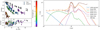 |
Fig. 6 Same as Fig. 5, but for the TGMdust model run with carbon grains. |
| In the text | |
|
Fig. 7 Vertical optical depth of the best-fit disk model with iron grains. Left panel: Radial optical depth profiles at selected wavelengths. Right panel: Optical depth spectra at the inner edges of each zone. |
| In the text | |
|
Fig. 8 Sketch of the disk of HD 144432, as seen by VLTI. We show the three ring-like structures, and the possible gaps between them. In the gaps we indicate two putative Jupiter mass planets. The cold outer disk, shown as a gray patch, cannot be constrained by our data. |
| In the text | |
|
Fig. 9 Concentration of various condensates (normalized to hydrogen atom number density) as a function of radius and temperature from our calculation using the thermo-chemical equilibrium code GGCHEM (Woitke et al. 2018). Top: plot showing the concentration using the photospheric elemental abundances of HD 144432. Bottom: plot showing the concentration using Solar elemental abundances. For clarity, we show a selection of the condensates: we plot only those species which are among the top three most abundant condensates for at least one temperature value. The T (r) relation follows our best-fit TGMdust model with iron grains. The gas pressure-temperature profile follows a power law with p = 3.16 × 10⁻² bar at the maximum temperature T = 2000 K, and p = 1.79 × 10⁻⁶ bar at the minimum temperature T = 277.5 K. |
| In the text | |
|
Fig. A.1 Calibrated MATISSE L band data sets. Left column: visibility as a function of the spatial frequency. Middle column: Closure phase as a function of the spatial frequency corresponding to the longest baselines of the triangles. Right panel: Correlated flux as a function of the wavelength. We also plot the single-dish spectrum, as the zero-baseline correlated spectrum. |
| In the text | |
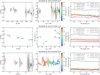 |
Fig. A.2 Same as Fig. A.1, but for the MATISSE M band data. |
| In the text | |
|
Fig. A.3 Same as Fig. A.1, but for the MATISSE N band data. We note that, as of DRS version 1.5.8, the sign convention of the N band phases are flipped with respect to the LM band phases (see also Gámez Rosas et al. 2022). This causes a 180° rotation of the N band images. This issue is no concern for us, as we do not use the N band closure phases in our modeling. |
| In the text | |
|
Fig. A.4 Calibrated GRAVITY data sets. Left column: visibility as a function of the spatial frequency. Right column: Closure phase as a function of the spatial frequency corresponding to the longest baselines of the triangles. |
| In the text | |
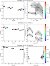 |
Fig. A.5 Same as Fig. A.4, but for the PIONIER data. |
| In the text | |
|
Fig. D.1 7–35 µm opacity curves of pyroxene, olivine, and various iron oxides, compared with the normalized Spitzer spectrum of HD 144432 (brown curve, AOR: 3587072). The Spitzer spectrum was normalized by dividing the data with the source function of our best-fit model. Optical constants of iron oxides were downloaded from the Jena Database of Optical Constants for Cosmic Dust (https://www.astro.uni-jena.de/Laboratory/OCDB/mgfeoxides.html). The original source for wüstite is Henning et al. (1995). Optical data for hematite and magnetite come from Amaury H.M.J. Triaud (unpublished). The opacity curves were generated with optool, using the distribution of hollow spheres (DHS) scattering theory. The upper boundary of the hollow sphere distribution (ƒmaχ) is 0.7. All curves are arbitrarily scaled and shifted to aid visual comparison. |
| In the text | |
|
Fig. D.2 N band opacity curves of the silicate minerals used in this work. Red color indicates the subset used in the final dust modeling. |
| In the text | |
|
Fig. D.3 Opacity curves in the full wavelength range of the data. Shown only the subset used in the final dust modeling, including iron and carbon as well. |
| In the text | |
|
Fig. F.1 Same as Fig. 1, but for a specfit solution corresponding to the dust mass fractions listed in Table F.1. |
| In the text | |
|
Fig. F.2 Same as Fig. 2, but for a specfit solution corresponding to the dust mass fractions listed in Table F.1. |
| In the text | |
|
Fig. G.1 Corner plot showing the posterior distributions of the MCMC samples from the run with iron grains. We note that in case of the surface densities and mass fractions we fit the logarithm of the quantities. |
| In the text | |
|
Fig. G.2 Best-fit model images at various data wavelengths with the TGMdust run with carbon grains. The brightness scaling is linear and homogeneous across all wavelengths. For a better perception of the fainter structural features, the images become saturated at 3.4 × 10⁻¹² W m−2 Hz−1 sr−1. The gray circles in the bottom left corner indicate the approximate beam size (estimated as 0.77λ/(Bp,max), where Bp,max is the maximum baseline length). |
| In the text | |
|
Fig. G.3 Radial surface brightness profiles of the disk corresponding to the best-fit TGMdust model with carbon grains. The shaded area around each curve is the 16–84 percentile range from the last 5000 samples of the chain. |
| In the text | |
|
Fig. G.4 Vertical optical depth of the best-fit disk model with carbon grains. Left panel: Radial optical depth profiles at selected wavelengths. Right panel: Optical depth spectra at the inner edges of each zone. |
| In the text | |
|
Fig. G.5 Corner plot showing the posterior distributions of the MCMC samples from the run with carbon grains. We note that in case of the surface densities and mass fractions we fit the logarithm of the quantities. |
| In the text | |
Current usage metrics show cumulative count of Article Views (full-text article views including HTML views, PDF and ePub downloads, according to the available data) and Abstracts Views on Vision4Press platform.
Data correspond to usage on the plateform after 2015. The current usage metrics is available 48-96 hours after online publication and is updated daily on week days.
Initial download of the metrics may take a while.