| Issue |
A&A
Volume 690, October 2024
|
|
|---|---|---|
| Article Number | A26 | |
| Number of page(s) | 12 | |
| Section | Galactic structure, stellar clusters and populations | |
| DOI | https://doi.org/10.1051/0004-6361/202449742 | |
| Published online | 26 September 2024 | |
Exploring the impact of a decelerating bar on transforming bulge orbits into disc-like orbits
1
Université de Strasbourg, CNRS, Observatoire astronomique de Strasbourg,
UMR 7550,
67000
Strasbourg,
France
2
Max-Planck-Institut für Astronomie,
Königstuhl 17,
69117
Heidelberg,
Germany
3
Canadian Institute for Theoretical Astrophysics, University of Toronto,
60 St. George Street,
Toronto,
ON
M5S 3H8,
Canada
4
Université Côte d’Azur, Observatoire de la Côte d’Azur, CNRS, Laboratoire Lagrange,
Nice,
France
Received:
26
February
2024
Accepted:
9
August
2024
Aims. The most metal-poor tail of the Milky Way ([Fe/H] ≤ −2.5) contains a population of stars on very prograde planar orbits, whose origins and evolution remain puzzling. One possible scenario is that they are shepherded by the bar from the inner Galaxy, where many of the old and low-metallicity stars in the Galaxy are located.
Methods. To investigate this scenario, we used test-particle simulations with an axisymmetric background potential plus a central bar model. The test particles were generated by an extended distribution function (EDF) model based on the observational constraints of bulge stars.
Results. According to the simulation results, a bar with a constant pattern speed is not efficient in terms of helping bring stars from the bulge to the solar vicinity. In contrast, when the model includes a decelerating bar, some bulge stars can gain rotation and move outwards as they are trapped in the bar’s resonance regions. The resulting distribution of shepherded stars heavily depends on the present-day azimuthal angle between the bar and the Sun. The majority of the low-metallicity bulge stars driven outwards are distributed in the first and fourth quadrants of the Galaxy with respect to the Sun and about 10% of them are within 6 kpc from us.
Conclusions. Our experiments indicate that the decelerating bar perturbation can be a contributing mechanism that may partially explain the presence of the most metal-poor stars with prograde planar orbits in the Solar neighbourhood, but it is unlikely to be the only one.
Key words: Galaxy: abundances / Galaxy: evolution / Galaxy: kinematics and dynamics / Galaxy: structure
© The Authors 2024
 Open Access article, published by EDP Sciences, under the terms of the Creative Commons Attribution License (https://creativecommons.org/licenses/by/4.0), which permits unrestricted use, distribution, and reproduction in any medium, provided the original work is properly cited.
This article is published in open access under the Subscribe to Open model. Subscribe to A&A to support open access publication.
1 Introduction
In the standard picture of galaxy formation, the innermost part of the Galaxy forms is likely to form first in the same phase as the assembly of the inner halo where most of the oldest and most metal-poor stars ([Fe/H] < −2.5) in the Galaxy are located (see e.g. Starkenburg et al. 2017; El-Badry et al. 2018). The Galactic old α-rich thick disc (with [Fe/H] ≳ −2.5) starts to form after the old bulge was built, and the thin disc is formed later, with predominately much younger and more metal-rich stars (see e.g. Bovy & Rix et al. 2012; Brook et al. 2012; Bland-Hawthorn & Gerhard 2016; Gallart et al. 2019; Xiang & Rix 2022).
Based on the broad-brush picture described above, we would expect the very low-metallicity stars ([Fe/H] < −2.5) in the solar neighborhood to likely be debris from the very early assembly phase of our Galaxy. Observations show that there are more stars in the very low-metallicity regime that have prograde orbits compared to those with retrograde orbits. Moreover, there is a population of prograde planar stars with strong rotation (azimuthal action, Jϕ > 1000 km s−1 kpc, which represents the angular momentum) and low-grade vertical motion (vertical action, Jz < 400 km s−1 kpc, which quantifies oscillations away from the Galactic plane), similar to the disc stars (Sestito et al. 2020; Di Matteo et al. 2020; Carollo et al. 2023; Fernández-Alvar et al. 2024). There are several possibilities of their origins under the debate (see, e.g. Sestito et al. 2020, 2021; Yuan et al. 2024). One possible scenario is that they can be transported by the bar from the inner Galaxy, as suggested by Dillamore et al. (2023), using a halo-like population under a short bar perturbation. Also, galactic bars are common in disc galaxies. The dynamical interplays between bar, disk, stellar, and dark matter halo are essential in galaxy evolution, but our understanding of these processes is far from complete (see, e.g. Sellwood & Wilkinson 1993; Sellwood 2014). In this work, we explore this possibility by tracing a peanut-shape bulge-like population generated in the framework of an extended distribution functions (EDFs) model under the perturbation of a long bar with different settings of pattern speeds. In order to make a comparison, we also carry out a simulation based on the pseudostars generated via a double power-law spheroidal distribution function (DF) model.
Schönrich & Binney (2009) modelled the Galaxy as a series of annuli with a chemical evolution process within which stars form from gas that they simultaneously enrich. Based on this work, Sharma et al. (2021) used the continuous disc model without distinct thin or thick disc to model the chemical evolution of the disc in the Galaxy. Similarly, Chen et al. (2023) used the galactic chemical evolution model with latest nucleosynthesis yields to model the chemical evolution with radial mixing in the Galactic disc. Both these works adopted a Schwarzschild DF f(ER, Jϕ, Ez) for the equilibrium model. Sanders & Binney (2015) updated the DFs with actions J as arguments, and introduced the concept of EDF for the Galactic disc components, namely, a density of stars in the five-dimensional space spanned by the actions J together with chemical abundances c = ([Fe/H], [Mg/Fe]). The EDF F(c, J) is thus a function of J and chemistry c. This EDF modelling method has also shown its ability in exploring the features of the stellar halo (Das & Binney 2016; Das et al. 2016).
The present work aims to investigate whether the bar can play a role in shaping the spatial distribution of the most metal-poor stars across the radial direction in the Galaxy. A test-particle simulation approach, with a background axisymmetric potential plus a bar perturbation, has been adopted to explore the capability of the bar in transporting the stellar population with [Fe/H] < −2.5 across the disc. The paper is organized as follows. The EDF model for generating initial pseudo-stars and compiling the total potential of the Galaxy is introduced in Section 2. The two kinds of bar models adopted in the test-particle simulation are presented in Section 2.4. The simulation results are shown in Section 3. In order to interpret the simulation results, observational data from Gaia Radial Velocity Sample (RVS; Katz et al. 2023) with the Pristine DR1 (Martin et al. 2023) are selected and the comparison with simulations are shown in Section 3.2. Finally, Section 4 summarises the paper and indicates directions for future work.
2 Modelling the extended distribution functions and simulation scheme
The origin and evolution of the most metal-poor stars population with prograde planar orbits is still a matter of debate. One of the possible scenarios is that these stars were born the inner Galaxy and brought outwards by the bar. To investigate this scenario, we carried out test-particle simulations with an axisymmetric background potential plus a central bar model. We introduce the model used to generate pseudo-stars and the potential of the bar below.
The Galaxy model used in this work includes two parts, an axisymmetric background and a central bar. The scheme of the test-particle approach generates the pseudo-stars based on the axisymmetric DFs, then integrates the pseudo-stars’ orbits in a potential system that includes the bar. It should be noticed that no selection function (SF) was adopted in our analysis, since the SF of the spectroscopic data used in this work is too complicated to model as they come from various observations. Nonetheless, our goal in this paper is to find a possible origin for these thin disclike stars in the solar vicinity, instead of quantitatively fitting our models to the observations.
2.1 The axisymmetric model of the Galaxy
In equilibrium, the DF can be taken as a function of the three action variables (Jr, Jz, Jϕ), which are isolating integrals of the motion (Binney & Tremaine 2008), where Jr quantifies the amplitude of radial excursions. Following the modelling work in Binney & Vasiliev (2023), an equilibrium Galaxy model can be defined by a superposition of similar DFs, including the dark halo, the stellar halo, the disc-like bulge, and four disc components, namely: a young disc, a middle-aged disc, and an old thin disc plus a high-α disc. The gravitational potential that these DFs jointly generate can then be found iteratively by the method introduced by Binney (2014) using the AGAMA package (Vasiliev 2019). The DF of each Galactic component is a specified function f(J) of the action integrals. In this model, the disc components have exponential DFs, which is physically reasonable throughout the action space, as compared to quasi-isothermal DFs. A double power law DF was used to model the stellar and dark halo. We do not have have access to much observational data via the centre of the Galaxy and, obviously, the central part of the Galaxy is non-axisymmetric. As a consequence (and to cover a range of possibilities), we used two different kinds of bulge models in our work: a truncated exponential DF (introduced in Section 2.2.1) and a double power law DF (introduced in Section 2.2.2). The total gravitational potential of the Galaxy is then derived from the DFs. The details of the descriptions of this Milky Way axisymmetric model can be found in Binney & Vasiliev (2023, 2024). The circular velocity generated from this axisymmetric potential is shown in the first panel of Figure 1. The black dots denote the circular velocity measurements from Classical Cepheids inside 10 kpc from the Galactic centre (Ablimit et al. 2020). Following our proposal in Li & Binney (2022b), a taper-exponential model is adopted for the young thin disc. The taper term in the model is a result of the sharp decline of the surface density of the gas inside the giant molecular ring, where the young disc stars have recently formed. Based on such a model, the disc components have a maximum circular velocity at 6–8 kpc away from the centre (as shown in the upper panel of Figure 1).
The EDF model in this work is based on the method introduced in Binney & Vasilie (2024), in which the EDF F(c, J) has J and chemistry c ≡ ([Fe/H], [Mg/Fe]) as its arguments. Because of the product rule, the EDF F(c, J) is found by multiplying the DF f(J) by the probability density P(c|J). This is the probability that a star with actions J has the chemistry c, i.e. F(c, J) = f(J)P(c|J). The detailed EDF bulge model will then be introduced in Sections 2.2 and 2.3.
2.2 DF of the bulge
2.2.1 Truncated exponential DF
Unlike the spheroidal bulge DF model used in Li & Binney (2022b) and Binney & Vasiliev (2023), this work follows Binney & Vasiliev (2024), which uses a truncated exponential DF model for the bulge as:
![$\[f(\mathbf{J})=f_\phi\left(J_\phi\right) f_r\left(J_r, J_\phi\right) f_z\left(J_z, J_\phi\right) f_{\mathrm{ext}}\left(J_\phi\right).\]$](/articles/aa/full_html/2024/10/aa49742-24/aa49742-24-eq1.png) (1)
(1)
In this model, the function fr controls the velocity dispersions σR and σϕ near the Galactic plane. The function fz controls both the thickness of the disc and the velocity dispersion σz. The factor fϕ generates a roughly exponentially declining surface density ∑(R) ≃ exp(-R/Rd). The factor fext truncates the disc at some outer radius. The detailed description of this model can be found in Binney & Vasiliev (2024).
There are two reasons for converting the bulge to a disclike component. One is that the observational data (Abdurro’uf et al. 2022) show that the bulge is almost entirely confined to Jϕ > 0 (Binney & Vasiliev 2024), which can naturally be represented by a disc-like model with prograde orbits. Secondly, a weak net rotation has been detected from RR Lyrae samples within ~3 kpc from the Galactic centre (Wegg et al. 2019; Li & Binney 2022a) and the metal-poor bulge sample from PIGS (Arentsen et al. 2020) which is probably the sign of a boxy/peanut bulge in the inner disc (see also Shen et al. 2010). Meanwhile, the dark matter halo can also show a net rotation due to the dynamical friction with the bar (Chiba & Schönrich 2022). In the design of our experiment, we chose a disc-like bulge model that can produce a net rotation in the inner part of the Galaxy to approximately simulate the boxy/peanut bulge, which a spheroidal DF model cannot represent. We modelled the bulge as a truncated exponential with large velocity dispersions and small radial extensions.
The velocity dispersion and surface density of the bulge according to the parameters listed in Table 1 is shown in the middle panel of Figure 1. The bottom panel shows the spatial distribution of the bulge in the (R, z) space, which is truncated at 6 kpc from the centre and has a peanut-like shape instead of a sphere.
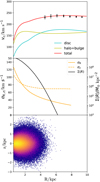 |
Fig. 1 Circular velocity within 10 kpc from the Galactic centre (upper panel), where the yellow curve represents the sum from the bulge and halo. The red curve denotes all four disc components. The black dots are from Ablimit et al. (2020) with the measurement from classical Cepheids. The velocity dispersion and surface density of the bulge are shown in the middle panel. The radial velocity dispersion σR drops much rapidly relative to the vertical velocity dispersion σz. The bottom panel shows the spatial distribution of the pseudo-stars in the (R, z) space for the bulge sample. The bulge is truncated within 6 kpc from the centre and has a peanut-like shape instead of a sphere. |
2.2.2 Double power law DF
To make our comparison, we carried out another simulation with a spheroidal DF for the bulge to test the ability of a decelerating bar to bring outwards the low metallicity stars. The perturbation and orbital integration schemes are the same with the truncated DF model. A double-power law model introduced in Li & Binney (2022a) is used to generate the pseudo-stars with the parameters shown in Table 2. In this case, the bulge stars do not have chemical information as those boxy/peanut bulge stars generated from the EDF model mentioned above.
The double-power law distribution function for the bulge is:
![$\[f=\frac{M}{\left(2 \pi J_0\right)^3} \frac{\left(1+\left[J_0 / h_J\right]^\gamma\right)^{\alpha / \gamma}}{\left(1+\left[J_0 / g_J\right]^\gamma\right)^{\beta / \gamma}} e^{-\left(g_J / J_{\text {cut }}\right)^\delta},\]$](/articles/aa/full_html/2024/10/aa49742-24/aa49742-24-eq2.png) (2)
(2)
where M is the normalization parameter relative to the mass of the bulge; α and β represent the inner and outer slopes in the phase space; and γ determines the steepness of the transition between the two parts. We ketp γ = 1 for the purposes of this work. Then, Jcut is the cut-off action which makes the value of the DF drop at large radii and δ is the steepness for that drop in order to keep the total mass always finite in the model. Finally, h(J) and g(J) are defined as:
![$\[\begin{aligned}& h(\mathbf{J})=\left(3-h_\phi-h_z\right) J_r+0.7\left(h_z ~J_z+h_\phi\left|J_\phi\right|\right), \\& g(\mathbf{J})=\left(3-g_\phi-g_z\right) J_r+0.7\left(g_z ~J_z+g_\phi\left|J_\phi\right|\right),\end{aligned}\]$](/articles/aa/full_html/2024/10/aa49742-24/aa49742-24-eq3.png) (3)
(3)
where hϕ and hz determine the velocity anisotropy at small radii and gϕ and gz determine the velocity anisotropy at large radii.
2.3 Chemical model of the bulge
The probability that a star with actions J has the chemistry c can be expressed as
![$\[P(\mathbf{c} {\mid} \mathbf{J})=\frac{\sqrt{\operatorname{det}(\mathbf{K})}}{2 \pi} \exp \left(\frac{1}{2}\left(\mathbf{c}-\mathbf{c}_{\mathbf{J}}\right)^T \cdot \mathbf{K} \cdot\left(\mathbf{c}-\mathbf{c}_{\mathbf{J}}\right)\right),\]$](/articles/aa/full_html/2024/10/aa49742-24/aa49742-24-eq4.png) (4)
(4)
where K is the 2 × 2 covariance Matrix, and cJ depends linearly on J as:
![$\[\mathbf{c}_{\mathbf{J}}=\mathbf{c}_0+\mathbf{C}\left(\mathbf{J}-\mathbf{J}_0\right) .\]$](/articles/aa/full_html/2024/10/aa49742-24/aa49742-24-eq5.png) (5)
(5)
Here, c0 contains two specific initial values for [Fe/H] and [Mg/Fe], and C is a 2 × 3 matrix which connects the action J and chemistry c. This probability can be approximated by a Gaussian distribution in c with mean and dispersion depending on J for both [Fe/H] and [Mg/Fe], according to the model from Binney & Vasiliev (2024).
Figure 2 shows the chemodynamical structure of the bulge by showing the relation between [Fe/H] and the three actions. The three panels are colour-coded in number density for JR, Jz, and Jϕ respectively. The bulge itself is modelled by a relatively young metal-rich component and most of our focus is on its old and very metal-poor parts in the simulations. The distribution extends to a lower metallicity, demonstrating that the dominant dependence of chemistry on action is aligned with Jz, where we have smaller values of Jz for metal-rich stars and larger Jz for metal-poor stars.
The parameters of the bulge EDF used in this work are listed in Table 3. The parameters in this chemical model are fitted by the observation of current bulge stars (Binney & Vasiliev 2024), with some minor modifications in this work. We made two modifications in the parameters. First, the value of Jext is lowered compared to the best fit value in Binney & Vasiliev (2024) to represent a smaller bulge 5 Gyr ago at the early epoch of the bar formation. Second, the matrix C is adjusted to show a stellar population deficient in metallicity 5 Gyr ago relative to current bulge population. We cannot represent the true chemical composition of the bulge 5 Gyr ago, especially for [Mg/Fe] because the current data is not enough to constrain models in the VMP region. However, since we are only interested in finding a possible origin of the metal-poor, thin-disc like stars, instead of tracing the α-element enhancement history in the central part of the Galaxy, it is reasonable to use these parameters for sampling the metallicity distribution of the bulge stars 5 Gyr ago.
Parameters used for the DF model of the bulge.
The parameters used for the spheroidal DF model of the bulge.
2.4 Bar models used in this work
We used two bar models in our simulations to investigate which is a better scenario for the Galaxy taking into account the observational constraints. First, a steadily rotating bar, with a given pattern speed Ωb, was modelled, following Chiba & Schönrich (2022) as:
![$\[\Phi_{\mathrm{b}}(r, \theta, \phi, t)=\Phi_{\mathrm{br}}(r) \sin ^2 \theta \cos m\left(\phi-\Omega_{\mathrm{b}} t\right),\]$](/articles/aa/full_html/2024/10/aa49742-24/aa49742-24-eq6.png) (6)
(6)
where (r, θ, ϕ) are the spherical coordinates. We only include the quadrupole term, m = 2, in this work.
The radial dependence of the bar potential Φbr(r) is
![$\[\Phi_{\mathrm{br}}(r)=-\frac{A v_{\mathrm{c}}^2}{2}\left(\frac{r}{r_{\mathrm{CR}}}\right)^2\left(\frac{b+1}{b+r / r_{\mathrm{CR}}}\right)^5,\]$](/articles/aa/full_html/2024/10/aa49742-24/aa49742-24-eq7.png) (7)
(7)
where A quantifies the strength of the bar and vc is the value of circular velocity in the solar vicinity, namely, vc = 235 km s−1. The parameter b describes the ratio between the bar scale length and the value of the co-rotation radius rCR. The parameters used in this work are given by Chiba & Schönrich (2022), with A = 0.02 and b = 0.28.
The pattern speed of the bar is Ωb = −35 km s−1 kpc−1 (Binney 2020; Chiba & Schönrich 2021). In the right-handed coordinate system used in this work, the pattern speed of the bar is negative and the bar rotates clockwise as the disc does. All parameters are summarized in Table 4.
Then, we also adopted a decelerating bar model similar to that used in Li et al. (2023), which is based on the model by Portail et al. (2017) using a made-to-measure method and updated parameters from Sormani et al. (2022). The difference with that work is that we impose the decelerating bar to end at a phase angle ϕ = 28° relative to the Sun, which is able to simulate the current morphology of the Galaxy (Wegg et al. 2015). In this work, the pattern speed of the bar drops from Ωb = −84km s−1 kpc−1 initially to Ωb = −30 km s−1 kpc−1 at the present time.
In this work, the pattern speed of the bar drops from Ωb = −84 km s−1 kpc−1 initially to Ωb = −30 km s−1 kpc−1 over 4 Gyr. Figure 3 shows the pattern speed as a function of time (solid black) along with its derivative (blue), namely, the slowing rate. The bar was introduced at T = 1Gyr and we increased the slowing rate linearly in time until T = 3Gyr, where we reduced the slowing down mechanism, such that ![$\[\dot{\Omega}_{\mathrm{p}}\]$](/articles/aa/full_html/2024/10/aa49742-24/aa49742-24-eq14.png) is null at T = 5Gyr. The resulting pattern speed varies smoothly from Ωb = −84 km s−1 kpc−1, with the largest variation occurring at T = 3Gyr. For comparison we also plot in dashed black the slowing bar model of Chiba et al. (2021) which is constrained by the Gaia data. Although our model has a larger maximum slowing rate, the two models are reasonably well matched. In Appendix A, we report the value of the dimensionless ‘speed parameter’ of our slowing bar model (Tremaine & Weinberg 1984; Chiba 2023). This parameter is lower than one, confirming that our slowing bar model evolves in the realistic ‘slow’ regime, where a substantial amount of stars are expected to be trapped in the main bar resonances.
is null at T = 5Gyr. The resulting pattern speed varies smoothly from Ωb = −84 km s−1 kpc−1, with the largest variation occurring at T = 3Gyr. For comparison we also plot in dashed black the slowing bar model of Chiba et al. (2021) which is constrained by the Gaia data. Although our model has a larger maximum slowing rate, the two models are reasonably well matched. In Appendix A, we report the value of the dimensionless ‘speed parameter’ of our slowing bar model (Tremaine & Weinberg 1984; Chiba 2023). This parameter is lower than one, confirming that our slowing bar model evolves in the realistic ‘slow’ regime, where a substantial amount of stars are expected to be trapped in the main bar resonances.
In addition, the mass and radial profile of the bar are evolving continuously during the simulation, reaching up to 2.5 and 1.5 times of the initial conditions, respectively, to roughly simulate the growth of the bar. We note that this change in amplitude of the potential will affect the width of trapped phase-space regions, but that the variation in angular momentum for each individual star (dominated by churning at corotation) is regulated by the variation of the pattern speed. This is because stars need to be carried around by a changing corotation to change significantly their guiding radii (without settling on more eccentric orbits).
It should also be noted that throughout this work, we neglect the self-gravity of the disc, which is the main caveat of test-particles simulations. Following Weinberg (1989), it is known that the resonant structure can be strengthened via self-gravitating processes (see also the discussions in Dootson & Magorrian 2022; Chiba 2023). This means that self-gravity will play a role in reshaping the diffusion of the disc, but this is beyond the scope of the present work, which is aimed at offering a preliminary qualitative analysis, rather than a quantitative one.
The orbital integration routine of AGAMA was adopted to compute the trajectories of all the mock stars for 5 Gyr in total and the trajectories were stored every 0.05 Gyr. In the first 1 Gyr, no bar was included and pseudo-stars only evolved in the axisymmetric background potential. The bar was added to the total potential at T = 1.0Gyr, with an initial radial profile and pattern speed of Ωb = −84 km s−1 kpc−1. Then, the bar started to decelerate and grow in mass and radial direction, reaching a pattern speed of Ωb = −30 km s−1 kpc−1 at the end of the simulation.
In Figure 4, we show the face-on contour maps of ⟨vR⟩ and Δvz for all the test particles at T = 3.0 Gyr and T = 5.0 Gyr for the steadily rotating and decelerating bar, respectively. The value of Δvz is the difference between ⟨vz⟩ for z > 0 and for z < 0. The upper panels correspond to the ⟨vR⟩ and Δvz distributions for the constant pattern speed bar model at T = 3.0 Gyr (left) and T = 5.0 Gyr (right). The ⟨vR⟩ plots clearly shows the signal of a quadruple feature in the centre of the Galaxy, whose strength differs very little between two snapshots. This is a consequence of the pseudo-stars reaching a near-equilibrium in the bar’s rotating frame. On the other hand, the distribution of Δvz does not show any signal of a quadruple feature even in the very centre of the Galaxy. This is due to the weak bar we choose in this model, which is not strong enough to disturb the orbits with high inclination with respect to the plane. Since the initial model of the bulge is disc-like with large velocity dispersions, the orbits with high inclination should make up a large fraction of the population of pseudo-stars.
The lower panels of Figure 4 show the distributions of ⟨vR⟩ and Δvz for the decelerating bar model at T = 3.0 Gyr and T = 5.0 Gyr, respectively. The pattern speed of the bar starts approximately with Ωb = −57 km s−1 kpc−1 at T = 3.0 Gyr and keeps decreasing to Ωb = −30 km s−1 kpc−1 at T = 5.0 Gyr. The quadruple feature at T = 3.0 Gyr is very prominent in both ⟨vR⟩ and Δvz plots. The ⟨vR⟩ values are several times larger than those of the constant pattern speed bar model, which suggests that our decelerating bar model can generate very strong quadruple features for all the pseudo-stars, including those with high orbital inclinations. The strong quadruple feature does not result from the deceleration but results from the forces generated by the bar, which are quite different among the two bar models. The m = 2 Fourier terms are shown in Figure 5 for both the constant rotating bar and the slowing down bar. The potential of the m = 2 terms for both models have similar outputs but are only about 2% of the background axisymmetric potential of the Galaxy. We also notice clear quadruple features at T = 5.0 Gyr in ⟨vR⟩ and Δvz between R ~ 5 kpc to R ~ 10 kpc that are related to the co-rotation resonance of the bar. This shows that the strong bar plays an important role in bringing the bulge stars to a disc region with resonance trapped orbits. Meanwhile, the small quadruple features inside R ~ 4 kpc may relate to the inner Lindblad resonance. The two families of orbits have a distinct separation between each other.
The evolution of the pseudo-stars under the influence of this decelerating bar is very clear in Figure 4. While at T = 3.0 Gyr, only one quadrupole feature is seen throughout the x − y plane, at T = 5.0 Gyr, a clear separation is seen between the inner and outer quadruple features, which shows the evolution process of the quadrupole structures for the pseudo-stars by the slowing down mechanism of the bar’s pattern speed. With the continuous decelerating of the bar’s pattern speed, the shape of the quadrupole structures continues to change without reaching a steady state in this simulation.
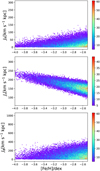 |
Fig. 2 The chemical model of the bulge used in this work showing the relation between [Fe/H] and actions. The three panels are colour-coded in number density for Jr, Jz, and Jϕ respectively. As we only focus on the metal-poor tail of the bulge, the x − axis is truncated at [Fe/H] = −2.5 in this plot. |
Parameters of the chemical models of the bulge.
Parameters used for the bar with steady rotation.
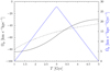 |
Fig. 3 Pattern speed as a function of time is shown in solid black line. The blue curve shows the derivative of the pattern speed. For comparison, the model from Chiba et al. (2021) is shown as a black dashed curve. |
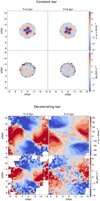 |
Fig. 4 Contours of ⟨vR⟩ and |
![$\[\Delta_{v_z}\]$](/articles/aa/full_html/2024/10/aa49742-24/aa49742-24-eq15.png)
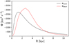 |
Fig. 5 m = 2 Fourier terms as a function of distance at z = 0 for both the constant rotating bar and the slowing down bar models. For the slowing down bar, the mass of the bar increases with a factor of 2.5 during the evolution of the bar while the mass of the bar keeps stable for the constant rotating bar. |
3 Simulation results and comparisons with observations
3.1 Model predictions
In this section, we try to interpret the simulation’s results for the boxy/peanut bulge model. Since we are interested in the origin and evolution of the low-metallicity stars in solar neighbourhood, we chose to focus on the test particles with [Fe/H] ≤ −2.5 from the simulations. The left panel in Figure 6 shows the initial condition of the low-metallicity particles selected according to the criteria introduced in Section 1 with −4 < [Fe/H] < −2.5. Their density distributions at T = 0 Gyr are shown in the top row. As the number on the top left indicates, the fraction of the low-metallicity particles relative to the whole sample is ~1.2%. In the central row, the mean value of azimuthal action, ⟨Jϕ⟩, is shown for each pixel instead of the stellar density. No pseudo-star displays an initial azimuthal action, Jϕ, larger than 1000 km s−1 kpc, which is reasonable since the pseudo stars are sampled by a truncated DF model. The bottom row shows the low-metallicity particles with Jz < 100 km s−1 kpc, which corresponds to a very thin-disc like behaviour. Only very few stars belong to this population, since we choose a large value for Jz0 in the bulge model.
The central column of Figure 6 shows the distribution of the low-metallicity particles at T = 3 Gyr for the constant bar model. Compared to the density distribution at T = 0 Gyr, the shape of the density contour becomes slightly elliptical in the central region, which is the consequence of the perturbation by the constant rotating bar. However, there is no obvious radial excursion of their orbits compared to their initial conditions. This feature is verified in the central row via colour-coded by ⟨Jϕ⟩ and shows that there are no particles that possess a Jϕ value larger than 1000 km s−1 kpc. The major difference between T = 3 Gyr and the initial condition lies in the bottom row. The number of stars with Jz < 100 km s−1 kpc increases from 393 to 12559. The right-most column shows their distribution at T = 5 Gyr, which resembles the result at T = 3 Gyr, only with a twist on the orientation of the bar’s major axis. The orange dot in this column marks the position of the Sun and the two dashed curves denote the 4 and 6 kpc circles away from the Sun. The central black line indicates the direction of the bar’s major axis, ϕ = 28° with respect to the Sun. We notice that the number of low-metallicity particles with Jz < 100 km s-1 kpc increases by a very small amount from T = 3 Gyr to T = 5 Gyr, which is explained by the pseudo-stars in this simulation reaching near-equilibrium in the bar’s rotating frame in less than 2 Gyr after the bar’s onset.
In the model of a decelerating bar, the left column of Figure 7 shows the distribution of the low-metallicity particles at T = 3 Gyr. Unlike the elliptical shape observed in the central region for a constant bar (Fig. 6), we observe the horseshoe orbits under a decelerating bar. This indicates that some orbits are elongated and brought outwards from the central region. To prove this, we plot in the central row the distribution of the low-metallicity particles with Jϕ > 1000 km s−1 kpc. Only a small portion of them (less than 1%) do actually show a disc-like behaviour even with Galacto-centric radius R > 10 kpc. The bottom row shows the particles with Jϕ > 1000 km s−1 kpc and Jz < 100km s−1 kpc, which corresponds to thin disc like properties. Contrary to the constant rotating bar, the decelerating bar is still in evolution at T = 3 Gyr. The low-metallicity particles show a quite different story at T = 5 Gyr and have two clear distinct regions in their distribution in x − y plane (right column). The pseudo-stars in the central region are still confined within the bulge, but with an elongated shape. On the other hand, two arc-shaped regions lying above and below the major axis of the bar show the pseudo-stars trapped by the co-rotation resonance of the bar. The central panel shows that 42% of the low-metallicity stars have Jϕ > 1000 km s−1 kpc at T = 5 Gyr, which is more than 60 times the fraction at T = 3 Gyr. 5% of the total number of the low-metallicity stars now have thin disc properties: Jϕ > 1000 km s−1 kpc, Jz < 100 km s−1 kpc. They are well confined by the co-rotation resonance of the bar. The two dashed circles mark the radius of 4 kpc and 6 kpc away from the Sun, which are the maximum radii at which most of the observed stars with [Fe/H] below − 2.5 are located. Comparing with the simulations, the fractions of the low-metallicity particles with disc-like behaviour located within these two circles are fairly low (shown in the right bottom panel). These proportions amount to about ~4% and ~10%, respectively, relative to the total number N = 6381 in this panel.
The decelerating bar has the ability to trap the most metal-poor bulge in the co-rotation resonance region, move them outwards, and endow them with a strong rotation, as shown in Figure 7. However, even in this idealized scenario, only a small fraction of the low-metallicity stars from the bulge are currently located in the solar vicinity at T = 5 Gyr. Most of the stars are trapped at the co-rotation resonance regions above and below the bar’s major axis in the (x, y) plane, which depends on the relative positions between the Sun and the bar. In the simulations, we set the evolution time to be relatively long, because the decelerating bar needs more time to evolve. Thus, some of the features can only be seen several Gyr after the bar onset. In our experiment, the pattern speed of the bar dropped to a value that is slightly smaller than the current estimated value in our Galaxy (Monari et al. 2019; Binney 2020; Chiba & Schönrich 2021; Clarke & Gerhard 2022; Leung et al. 2023; Lucey et al. 2023; Gaia Collaboration 2023a) at T = 5 Gyr. Consequently, the corotation radius stops increasing and the migration of the perturbed stars ceases, we thus set T = 5 Gyr as the end of the simulation.
To figure out the possible mechanism of the decelerating bar in shaping the bulge distribution seen in Figure 7, we look into the resonance frequency as a function of planar radius in Figure 8. The solid cyan line corresponds to the bar’s pattern speed used in the constant rotating bar model. The two dashed blue lines mark the initial and final pattern speed in the decelerating bar model. The black solid curve is the azimuthal frequency, Ω, based on the axisymmetric potential used in this work. Thus, the intersections between the bar’s pattern speeds and Ω denote the location of co-rotation resonance. The intersections of the Ω + κ/2 and the bar’s pattern speeds denote the OLR (Outer Lindblad resonance) shown as the dashed curve. The similar intersection of Ω − κ/2 denotes the ILR (Inner Lindblad resonance) as the dashed-dotted curve. The co-rotation radius of the constant rotating bar is at R ≈ 7 kpc, which is further outside than the sampled particles. The only possible influence of a resonance on the pseudo-stars is the ILR. Since the pattern speed does not change in this constant pattern speed model, the resonance trapped radius also stays stable throughout the simulation, which makes stars confined within the initial truncated radius (as shown in the upper panel of Figure 6). The case for the decelerating bar is far more interesting. With a larger initial value of the pattern speed, the co-rotation radius for this model is less than 3 kpc from the centre, well within the sampled pseudostars’ spatial region. The direct consequence is that a fraction of pseudo-stars are trapped by the co-rotation resonance since the start of the simulation. As the bar’s pattern speed decreases, the co-rotation radius increases to R ≈ 8 kpc and the number of pseudo-stars that are trapped with the co-rotation resonance also increases. Those trapped stars are then brought outwards with the moving of the bar’s co-rotation trapped region.
The discussions on dynamical resonances of the bar in this section are mainly focused on the co-rotation resonance. However, the co-rotation is not the only way that can transfer angular momentum to stars, which can be verified by the data in the lower panel of Figure 7. Here, we can see that some pseudo-stars are fully outside the co-rotation resonance zone of the bar. Another work with similar purposes has been carried out by Saha et al. (2012) via N-body simulations, studying the angular momentum transfer from the bar to an initially isotropic non-rotating small classical bulge, bringing stars as far away as the Solar neighbourhood. These authors also concluded that the angular momentum transfer takes place through the resonances of the bar, but mainly through the ILR. The difference between the two works is that the co-rotation resonance of the bar in Saha et al. (2012) is outside the radius that confine most bulge particles; thus, only the ILR plays an important role in transferring the angular momentum to the particles. On the contrary, in our work, the initial co-rotation resonance of the bar is inside the bulge region, leading to more co-rotation resonance trapping of the particles. In our work, the ILR actually also transfers angular momentum to the particles, but with very small contributions. More detailed work should be carried out in the future to study the ability of various bar resonances to transfer angular momentum to the stars in a model akin to the one presented here.
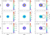 |
Fig. 6 Very-low-metallicity stars ([Fe/H] ≤ −2.5) for the boxy/peanut bulge model in the constant rotating bar at T = 3 Gyr and T = 5 Gyr in the middle and right panels, respectively. The central row is colour-coded by Jϕ. The bottom row shows the low-metallicity particles with Jz < 100 km s−1 kpc. The orange dot in the right panel marks the position of the Sun, while the two dashed curves denote the distances at 4 and 6 kpc from the Sun. The thick line denotes the direction of major axis of the bar at T = 5 Gyr. Within this constant bar model, no test particles can exceed a value of 1000 km s−1 kpc for the value of Jϕ. |
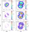 |
Fig. 7 Very-low-metallicity stars (same as Fig. 6) for the boxy/peanut bulge model under the decelerating bar at T = 3 Gyr and T = 5 Gyr, respectively. In the central row, we plot the distribution for the low-metallicity particles with Jϕ > 1000 km s−1 kpc. The bottom row shows the particles with Jϕ > 1000 km s−1 kpc & Jz < 100 km s−1 kpc. The orange dot in the right panel marks the position of the Sun and the two dashed curves denote the distances at 4 and 6 kpc from the Sun. The pseudo-stars in the central region of the Galaxy evolve sharply within the simulation time. Some of these stars are driven outwards by the decelerating bar with the co-rotation trapping. It is clear that at T = 5 Gyr, about 6000 pseudo-stars show a feature of rotationdominated orbits with very low metallicities. |
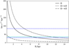 |
Fig. 8 Frequency of Ω ± κ/2 derived from the background potential as a function of planar radius. The solid cyan line denotes to the bar’s pattern speed used in the constant rotating bar model. The co-rotation radius is defined as the planar radius at the intersection between the frequency curve and the pattern speed curve. The dashed blue lines mark the initial and final pattern speed in the decelerating bar model, which shows the change of co-rotation radius during 6 Gyrs. The stars trapped by the bar thus migrate outwards with time until the pattern speed reaches a stable value and the co-rotation radius stops increasing. |
3.2 Data and comparisons
To compare with the model prediction, we build our sample by cross-matching the Gaia DR3 Radial Velocity Sample (RVS; Katz et al. 2023) with the photometric metallicity catalogues based on the narrow-band CaHK magnitudes from the Pristine survey (Martin et al. 2023). There are two catalogues used in this work: 1) the Pristine-Gaia synthetic catalogue, which uses the CaHK magnitude built from Gaia BP/RP spectro-photometry (Gaia Collaboration et al. 2023b) and 2) the Pristine DR1 based on the real CaHK measurements taken by the Canada-France-Hawaii Telescope, which has a smaller number of stars, but a higher signal-to-noise ratio (S/N) compared to the first catalogue. By combining these two samples, we were able to include as many low-metallicity RVS stars as possible and take the metallicity values with smaller uncertainties when stars were duplicated.
We first select a low-metallicity sample from the giant solutions from Pristine DR1: FeH_Pristine > −4.0 and FeH_Pristine ≤ −2.5 and mcfrac_Pristine > 0.8 and FeH_Pristine_84th − FeH_Pristine_16th < 0.6. We note that the metallicity column from the Pristine-Gaia synthetic catalogue is FeH_CaHKsyn. To obtain a confident sample of low-metallicity stars, here we use a relatively strict cut in photometric uncertainties (δ[Fe/H]phot < 0.3) and apply the following quality cuts according to the recommended practice from Martin et al. (2023):
E(B-V) < 0.3, relatively strict cut to remove stars with heavy extinctions.
Pvar ≤ 0.3, relatively strict cut to remove potentially variable stars.
RUWE < 1.4 from the Gaia quality cuts.
C* < 3× σC*, relatively loose cut to remove stars deviate more than 3σ from the corrected flux excess (Riello et al. 2021).
We then filtered out the sample using parallax_over_error ≥ 5 and manually selected stars around the giant branch from the colour absolute magnitude diagram. This procedure discards the dwarf stars that get into the sample from the previous selection criteria, which suffer from more severe contamination from the metal-rich population. The final sample has 3259 stars that have uncertainty in distance less than 20%.
A comparison between the observation and simulation in the (Jϕ, Jz) space is shown in Figure 9. The colour-coded contours show the very low-metallicity stars in the simulation with Jϕ and Jz values at T = 5Gyr in the decelerating bar model. The density increases by a factor of 2 between adjacent contours. We see a clear bimodal distribution, where half of the particles keep low Jϕ corresponding to those that remain close to the Galactic center (see first row of Fig. 7); whereas the other half are peaked between Jϕ = 1000 ~ 2000 km s−1 kpc and are located in the arches further from the center shown in Fig. 7. The final low-metallicity RVS sample is plotted as light purple dots, and the stars in the selection box from Sestito et al. (2020) are highlighted as blue dots. It is clear that the selected rotationdominated stars overlap with the population with strong rotation from the model. To test the ability of a decelerating bar to bring outwards the low metallicity stars, we adopted another model (introduced in Section 2.2.2), where those stars are originally distributed in a spheroid. The results from a spheroidal bulge also have a clear bi-modalitiy distribution and a second peak that overlaps with the observed stars in the selection box (see the lower panel of Figure 9). We note that the final Jz distribution from the spheroidal bulge model is more scattered than that from the peanut-shape bulge. These results show that the decelerating bar has the ability to bring the most metal-poor stars outwards to thin disc-like orbits, regardless of the model used to generate the mock catalogue. It should be noticed that the spheroidal bulge stars do not have chemical information, thus, we give a plot of all the pseudo-stars in the lower panel of Figure 9.
In Figure 10, we plot the spatial distribution of the final sample shown as light purple dots, including 317 stars (blue dots) selected with 1000 < Jϕ < 2500 km s−1 kpc & Jz < 400 km s−1 kpc (Sestito et al. 2020). As discussed in Sec. 3.1, the majority of the stars moving outwards are distributed in the fourth quadrant of the Galaxy and are outside of the solar circles; whereas the observed stars are mostly within. Moreover, the observed stars selected in this work are confined away from the Galactic centre due to the heavy extinction region near the Galactic plane, shown in the (x, z) space in the bottom panel. In summary, the spatial distributions between the model and the observations have fairly small overlaps in space. It is difficult to explain the key origins of these stars observed in the Solar neighbourhood solely via the mechanism of a decelerating bar.
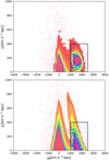 |
Fig. 9 Final Jϕ-Jz distribution for both the simulation result with a decelerating bar (with a boxy/peanut bulge) and the observational data, shown in the upper panel. The contours show the distribution for very metal-poor pseudo-stars, with a clear bi-modal distribution. The pseudo-stars with Jϕ > 1000 denote the population that is driven outwards by the decelerating bar. The black box represents the selection criteria and the blue stars represent the same stars as those plotted in Figure 10. The simulation result coincides with the observations well. In order to make a comparison with another bulge model, the result from another experiment with a spheroidal bulge is shown in the lower panel. The bi-modality distribution is still clear in this second experiment. |
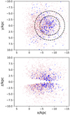 |
Fig. 10 Space distribution of all the observational data used in this work. The red dot shows all the low-metallicity stars based on CaHK magnitudes and the blue dot shows the stars with rotation-dominated orbits 1000 < Jϕ < 2500 km s−1 kpc & Jz < 400 km s−1 kpc. The two circles are the same with those given in the right-most panel of Figure 7. |
4 Conclusion
In this paper, we carried out test-particle simulations aimed at elucidating the possible origin of the low-metallicity stars with the thin disc-like behaviour that was recently observed (Sestito et al. 2020; Yuan et al. 2024).
We adopted two different bar models for the simulations. Under the constant pattern speed bar model, the pseudo-stars were nearly able to retain their initial conditions within the central regions in the Galaxy and have no migration outwards across the disc as time evolves. In addition, the number of stars with Jz < 100 km s−1 kpc increases by a very small amount, from T = 3 Gyr to T = 5 Gyr, which means that the constant bar reaches a near-equilibrium state earlier than T = 2 Gyr after the bar appears. The scenario of the decelerating bar model is very different. According to the simulation results, the decelerating bar shows the ability to bring the bulge stars outwards by trapping them in the resonance regions. The co-rotation resonance radius of the decelerating bar model is less than 3 kpc from the centre initially, which allows for a fraction of pseudo-stars to be trapped by the bar from the start of the emergence of the bar in the simulation. With the decrease in the bar’s pattern speed and the increase of the co-rotation radius, the number of pseudostars that are trapped at the co-rotation resonance increases and these stars also migrate outwards as time evolves. We note that the decelerating bar needs more time to evolve, and the number of stars driven outwards only increases drastically several Gyr after the bar is created. It is possible that the other resonances of the bar also have the ability to transfer angular momentum to stars, such as the ILR (see Saha et al. (2012) for example). More detailed works should be carried in the future to verify the capability of transferring angular momentum to the stars by various resonances of the bar.
We then compared our simulation predictions with the Gaia DR3 RVS sample, with its metallicities based on CaHK magnitudes. The results show that the decelerating bar is capable of moving stars from the inner Galaxy outwards on very prograde planar orbits. However, based on the relative positions between the bar and the Sun, only a small fraction of these low-metallicity pseudo bulge stars move to the Solar vicinity: about 10% of the stars with disc behaviours are located within 6 kpc from us, and only about 4% within 4 kpc. This possibly indicates that the decelerating bar is unlikely to be the only mechanism for the stars of interests in the Solar neighbourhood, consistent with our prior results, published in Yuan et al. (2024). Most of the migrated stars in our simulation are located in the direction towards the Galactic center where high-quality measurements of photometric metallicities are lacking due to heavy extinction. We note that we here have focussed on the mystery of planar low-metallicity stars, but the effect of the decelerating bar can similarly (or even more strongly) impact metal-rich stars.
The exact percentages mentioned above can of course depend on the precise way in which the pattern speed of the bar has decelerated. Moreover, our model does not take into account the possibility that short-lived recurring spiral arms with different pattern speeds could have their resonances overlapping with the bar’s resonances at different radii (Sellwood & Binney 2002; Minchev & Famaey 2010) and hence enhance the migration of the old stars. Observationally, it had already been noted (e.g. Minchev et al. 2014; Lagarde et al. 2021) in past studies that the oldest stars of the high-α metal-poor, thick disk tend to have planar orbits with low vertical velocity dispersions compared to slightly younger ones, which had been attributed to a similar migration mechanism.
Moreover, there are a few caveats with the present model. The boxy/peanut bulge can itself be a manifestation resulting from bar instability, meaning that its present-day structure is not necessarily representative of its past one in a growing bar model, which is why it is reassuring that similar results were obtained for a different DF. In addition, the slowing bar model adopted in this paper has not been adjusted to fit the data. The maximum slowing rate is slightly larger than the recent measurement (Chiba et al. 2021) and the final pattern speed of our bar model is smaller than current observational values. These settings enable stars to move over a very large radius range from the very inner Galaxy to our vicinity, which is probably not very realistic. Furthermore, recent studies indicate that the presence of gas may significantly slow down or even stop the slowdown of galactic bars (Beane et al. 2023). To further verify the predictions from our simulations, the upcoming WEAVE survey (Jin et al. 2023) and the forthcoming 4MOST survey (de Jong et al. 2019) will fill the data in the sparse region towards the Galactic centre. In the long term, the studies of stars in these obscured regions will be greatly benefit from a near-infrared (NIR) astrometric survey such as GaiaNIR (Hobbs et al. 2016).
Acknowledgements
CL, AS, BF, GM, GK, and VH acknowledge funding from the ANR grant ANR-20-CE31-0004 (MWDisc). ZY, NFM, BF, GM, and RAI acknowledge funding from the European Research Council (ERC) under the European Union’s Horizon 2020 research and innovation programme (grant agreement No. 834148). ZY, NFM, GK, and VH gratefully acknowledge support from the French National Research Agency (ANR) funded project “Pristine” (ANR-18-CE31-0017). RC thanks support by the Natural Sciences and Engineering Research Council of Canada (NSERC), [funding reference #DIS-2022-568580]. This work presents results from the European Space Agency (ESA) space mission Gaia. Gaia data are being processed by the Gaia Data Processing and Analysis Consortium (DPAC). Funding for the DPAC is provided by national institutions, in particular the institutions participating in the Gaia MultiLateral Agreement (MLA). The Gaia mission website is https://www.cosmos.esa.int/gaia. The Gaia archive website is https://archives.esac.esa.int/gaia.
Appendix A Speed parameter
The response of stars to a slowing bar depends crucially on the bar’s slowing rate (Tremaine & Weinberg 1984; Chiba et al. 2021). From a dynamical viewpoint, whether the bar is slowing down ‘slowly’ or ‘rapidly’ is classified by the dimensionless speed parameter s (Tremaine & Weinberg 1984), which is the ratio of the characteristic libration period to the time the resonance takes to move by its width (Chiba 2023). When 0 < s < 1, the bar’s resonance moves slowly such that a finite volume of phase space surrounding the resonance is trapped (the slow regime). Beyond s = 1, the evolution is too fast for any star to remain trapped in resonance (the fast regime).
Figure A.1 shows the speed parameter of our slowing bar model for the corotation resonance. We calculated s for three different radial and vertical actions (Jr, Jz) = (0, 0), (50, 0), (50, 50)km s−1 kpc, which are integral of motions at the corotation resonance (the fast actions). For all three actions, the speed parameter is below unity, indicating that our slowing bar model resonantly traps and drags a sizeable amount of stars at corotation. The speed parameter initially rises and later decays, following the variation in the bar’s slowing rate ![$\[\dot{\Omega}_{\mathrm{p}}\]$](/articles/aa/full_html/2024/10/aa49742-24/aa49742-24-eq16.png) (t) (cf. Fig. 3). The bump at T = 3Gyr is inherited from the behaviour of
(t) (cf. Fig. 3). The bump at T = 3Gyr is inherited from the behaviour of ![$\[\dot{\Omega}_{\mathrm{p}}\]$](/articles/aa/full_html/2024/10/aa49742-24/aa49742-24-eq17.png) .
.
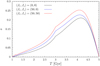 |
Fig. A.1 Speed parameter of our slowing bar model for the corotation resonance. The black, blue, and red curves denote the computation for (Jr, Jz) = (0, 0), (50, 0), (50, 50)km s−1 kpc, respectively. |
References
- Abdurro’uf, Accetta, K., Aerts, C., et al. 2022, ApJS, 259, 35 [NASA ADS] [CrossRef] [Google Scholar]
- Ablimit, I., Zhao, G., Flynn, C., & Bird, S. A. 2020, ApJ, 895, L12 [Google Scholar]
- Arentsen, A., Starkenburg, E., Martin, N. F., et al. 2020, MNRAS, 491, L11 [Google Scholar]
- Beane, A., Hernquist, L., D’Onghia, E., et al. 2023, ApJ, 953, 173 [NASA ADS] [CrossRef] [Google Scholar]
- Binney, J. 2014, MNRAS, 440, 787 [Google Scholar]
- Binney, J. 2020, MNRAS, 495, 895 [NASA ADS] [CrossRef] [Google Scholar]
- Binney, J., & Tremaine, S. 2008, Galactic Dynamics: Second Edition (Princeton, NJ, USA: Princeton University Press) [Google Scholar]
- Binney, J., & Vasiliev, E. 2023, MNRAS, 520, 1832 [NASA ADS] [CrossRef] [Google Scholar]
- Binney, J., & Vasiliev, E. 2024, MNRAS, 527, 1915 [Google Scholar]
- Bland-Hawthorn, J., & Gerhard, O. 2016, ARA&A, 54, 529 [Google Scholar]
- Bovy & Rix, J., Rix, H.-W., Liu, C., et al. 2012, ApJ, 753, 148 [NASA ADS] [CrossRef] [Google Scholar]
- Brook, C. B., Stinson, G. S., Gibson, B. K., et al. 2012, MNRAS, 426, 690 [Google Scholar]
- Carollo, D., Christlieb, N., Tissera, P. B., & Sillero, E. 2023, ApJ, 946, 99 [NASA ADS] [CrossRef] [Google Scholar]
- Chen, B., Hayden, M. R., Sharma, S., et al. 2023, MNRAS, 523, 3791 [NASA ADS] [CrossRef] [Google Scholar]
- Chiba, R. 2023, MNRAS, 525, 3576 [NASA ADS] [CrossRef] [Google Scholar]
- Chiba, R., & Schönrich, R. 2021, MNRAS, 505, 2412 [NASA ADS] [CrossRef] [Google Scholar]
- Chiba, R., & Schönrich, R. 2022, MNRAS, 513, 768 [NASA ADS] [CrossRef] [Google Scholar]
- Chiba, R., Friske, J. K. S., & Schönrich, R. 2021, MNRAS, 500, 4710 [Google Scholar]
- Clarke, J. P., & Gerhard, O. 2022, MNRAS, 512, 2171 [NASA ADS] [CrossRef] [Google Scholar]
- Das, P., & Binney, J. 2016, MNRAS, 460, 1725 [NASA ADS] [CrossRef] [Google Scholar]
- Das, P., Williams, A., & Binney, J. 2016, MNRAS, 463, 3169 [NASA ADS] [CrossRef] [Google Scholar]
- de Jong, R. S., Agertz, O., Berbel, A. A., et al. 2019, The Messenger, 175, 3 [NASA ADS] [Google Scholar]
- Dillamore, A. M., Belokurov, V., Evans, N. W., & Davies, E. Y. 2023, MNRAS, 524, 3596 [NASA ADS] [CrossRef] [Google Scholar]
- Di Matteo, P., Spite, M., Haywood, M., et al. 2020, A&A, 636, A115 [NASA ADS] [CrossRef] [EDP Sciences] [Google Scholar]
- Dootson, D., & Magorrian, J. 2022, arXiv e-prints [arXiv:2205.15725] [Google Scholar]
- El-Badry, K., Bland-Hawthorn, J., Wetzel, A., et al. 2018, MNRAS, 480, 652 [NASA ADS] [CrossRef] [Google Scholar]
- Fernández-Alvar, E., Kordopatis, G., Hill, V., et al. 2024, A&A, 685, A151 [NASA ADS] [CrossRef] [EDP Sciences] [Google Scholar]
- Gaia Collaboration (Drimmel, R., et al.) 2023a, A&A, 674, A37 [Google Scholar]
- Gaia Collaboration (Montegriffo, P., et al.) 2023b, A&A, 674, A33 [Google Scholar]
- Gallart, C., Bernard, E. J., Brook, C. B., et al. 2019, Nat. Astron., 3, 932 [NASA ADS] [CrossRef] [Google Scholar]
- Hobbs, D., Høg, E., Mora, A., et al. 2016, arXiv e-prints [arXiv:1609.07325] [Google Scholar]
- Jin, S., Trager, S. C., Dalton, G. B., Aguerri, J. A. L., & Drew, J. E. 2023, MNRAS, arXiv e-prints [arXiv:2212.03981] [Google Scholar]
- Katz, D., Sartoretti, P., Guerrier, A., et al. 2023, A&A, 674, A5 [NASA ADS] [CrossRef] [EDP Sciences] [Google Scholar]
- Lagarde, N., Reylé, C., Chiappini, C., et al. 2021, A&A, 654, A13 [NASA ADS] [CrossRef] [EDP Sciences] [Google Scholar]
- Leung, H. W., Bovy, J., Mackereth, J. T., et al. 2023, MNRAS, 519, 948 [Google Scholar]
- Li, C., & Binney, J. 2022a, MNRAS, 510, 4706 [NASA ADS] [CrossRef] [Google Scholar]
- Li, C., & Binney, J. 2022b, MNRAS, 516, 3454 [NASA ADS] [CrossRef] [Google Scholar]
- Li, C., Siebert, A., Monari, G., Famaey, B., & Rozier, S. 2023, MNRAS, 524, 6331 [NASA ADS] [CrossRef] [Google Scholar]
- Lucey, M., Pearson, S., Hunt, J. A. S., et al. 2023, MNRAS, 520, 4779 [NASA ADS] [CrossRef] [Google Scholar]
- Martin, N. F., Starkenburg, E., Yuan, Z., et al. 2023, A&A submitted [arXiv:2308.01344] [Google Scholar]
- Minchev, I., & Famaey, B. 2010, ApJ, 722, 112 [Google Scholar]
- Minchev, I., Chiappini, C., Martig, M., et al. 2014, ApJ, 781, L20 [Google Scholar]
- Monari, G., Famaey, B., Siebert, A., Wegg, C., & Gerhard, O. 2019, A&A, 626, A41 [NASA ADS] [CrossRef] [EDP Sciences] [Google Scholar]
- Portail, M., Gerhard, O., Wegg, C., & Ness, M. 2017, MNRAS, 465, 1621 [NASA ADS] [CrossRef] [Google Scholar]
- Riello, M., De Angeli, F., & Evans. 2021, A&A, 649, A3 [NASA ADS] [CrossRef] [EDP Sciences] [Google Scholar]
- Saha, K., Martinez-Valpuesta, I., & Gerhard, O. 2012, MNRAS, 421, 333 [Google Scholar]
- Sanders, J. L., & Binney, J. 2015, MNRAS, 449, 3479 [NASA ADS] [CrossRef] [Google Scholar]
- Schönrich, R., & Binney, J. 2009, MNRAS, 396, 203 [Google Scholar]
- Sellwood, J. A. 2014, Rev. Mod. Phys., 86, 1 [Google Scholar]
- Sellwood, J. A., & Binney, J. J. 2002, MNRAS, 336, 785 [Google Scholar]
- Sellwood, J. A., & Wilkinson, A. 1993, Rep. Progr. Phys., 56, 173 [CrossRef] [Google Scholar]
- Sestito, F., Martin, N. F., Starkenburg, E., et al. 2020, MNRAS, 497, L7 [Google Scholar]
- Sestito, F., Buck, T., Starkenburg, E., et al. 2021, MNRAS, 500, 3750 [Google Scholar]
- Sharma, S., Hayden, M. R., & Bland-Hawthorn, J. 2021, MNRAS, 507, 5882 [NASA ADS] [CrossRef] [Google Scholar]
- Shen, J., Rich, R. M., Kormendy, J., et al. 2010, ApJ, 720, L72 [NASA ADS] [CrossRef] [Google Scholar]
- Sormani, M. C., Gerhard, O., Portail, M., Vasiliev, E., & Clarke, J. 2022, MNRAS, 514, L1 [NASA ADS] [CrossRef] [Google Scholar]
- Starkenburg, E., Oman, K. A., Navarro, J. F., et al. 2017, MNRAS, 465, 2212 [NASA ADS] [CrossRef] [Google Scholar]
- Tremaine, S., & Weinberg, M. D. 1984, MNRAS, 209, 729 [Google Scholar]
- Vasiliev, E. 2019, MNRAS, 482, 1525 [Google Scholar]
- Wegg, C., Gerhard, O., & Portail, M. 2015, MNRAS, 450, 4050 [NASA ADS] [CrossRef] [Google Scholar]
- Wegg, C., Gerhard, O., & Bieth, M. 2019, MNRAS, 485, 3296 [NASA ADS] [CrossRef] [Google Scholar]
- Weinberg, M. D. 1989, MNRAS, 239, 549 [NASA ADS] [CrossRef] [Google Scholar]
- Xiang, M., & Rix, H.-W. 2022, Nat, 603, 599 [NASA ADS] [CrossRef] [Google Scholar]
- Yuan, Z., Li, C., Martin, N. F., et al. 2024, A&A, submitted [arXiv:2311.08464] [Google Scholar]
All Tables
All Figures
|
Fig. 1 Circular velocity within 10 kpc from the Galactic centre (upper panel), where the yellow curve represents the sum from the bulge and halo. The red curve denotes all four disc components. The black dots are from Ablimit et al. (2020) with the measurement from classical Cepheids. The velocity dispersion and surface density of the bulge are shown in the middle panel. The radial velocity dispersion σR drops much rapidly relative to the vertical velocity dispersion σz. The bottom panel shows the spatial distribution of the pseudo-stars in the (R, z) space for the bulge sample. The bulge is truncated within 6 kpc from the centre and has a peanut-like shape instead of a sphere. |
| In the text | |
|
Fig. 2 The chemical model of the bulge used in this work showing the relation between [Fe/H] and actions. The three panels are colour-coded in number density for Jr, Jz, and Jϕ respectively. As we only focus on the metal-poor tail of the bulge, the x − axis is truncated at [Fe/H] = −2.5 in this plot. |
| In the text | |
|
Fig. 3 Pattern speed as a function of time is shown in solid black line. The blue curve shows the derivative of the pattern speed. For comparison, the model from Chiba et al. (2021) is shown as a black dashed curve. |
| In the text | |
|
Fig. 4 Contours of ⟨vR⟩ and |
| In the text | |
|
Fig. 5 m = 2 Fourier terms as a function of distance at z = 0 for both the constant rotating bar and the slowing down bar models. For the slowing down bar, the mass of the bar increases with a factor of 2.5 during the evolution of the bar while the mass of the bar keeps stable for the constant rotating bar. |
| In the text | |
|
Fig. 6 Very-low-metallicity stars ([Fe/H] ≤ −2.5) for the boxy/peanut bulge model in the constant rotating bar at T = 3 Gyr and T = 5 Gyr in the middle and right panels, respectively. The central row is colour-coded by Jϕ. The bottom row shows the low-metallicity particles with Jz < 100 km s−1 kpc. The orange dot in the right panel marks the position of the Sun, while the two dashed curves denote the distances at 4 and 6 kpc from the Sun. The thick line denotes the direction of major axis of the bar at T = 5 Gyr. Within this constant bar model, no test particles can exceed a value of 1000 km s−1 kpc for the value of Jϕ. |
| In the text | |
|
Fig. 7 Very-low-metallicity stars (same as Fig. 6) for the boxy/peanut bulge model under the decelerating bar at T = 3 Gyr and T = 5 Gyr, respectively. In the central row, we plot the distribution for the low-metallicity particles with Jϕ > 1000 km s−1 kpc. The bottom row shows the particles with Jϕ > 1000 km s−1 kpc & Jz < 100 km s−1 kpc. The orange dot in the right panel marks the position of the Sun and the two dashed curves denote the distances at 4 and 6 kpc from the Sun. The pseudo-stars in the central region of the Galaxy evolve sharply within the simulation time. Some of these stars are driven outwards by the decelerating bar with the co-rotation trapping. It is clear that at T = 5 Gyr, about 6000 pseudo-stars show a feature of rotationdominated orbits with very low metallicities. |
| In the text | |
|
Fig. 8 Frequency of Ω ± κ/2 derived from the background potential as a function of planar radius. The solid cyan line denotes to the bar’s pattern speed used in the constant rotating bar model. The co-rotation radius is defined as the planar radius at the intersection between the frequency curve and the pattern speed curve. The dashed blue lines mark the initial and final pattern speed in the decelerating bar model, which shows the change of co-rotation radius during 6 Gyrs. The stars trapped by the bar thus migrate outwards with time until the pattern speed reaches a stable value and the co-rotation radius stops increasing. |
| In the text | |
|
Fig. 9 Final Jϕ-Jz distribution for both the simulation result with a decelerating bar (with a boxy/peanut bulge) and the observational data, shown in the upper panel. The contours show the distribution for very metal-poor pseudo-stars, with a clear bi-modal distribution. The pseudo-stars with Jϕ > 1000 denote the population that is driven outwards by the decelerating bar. The black box represents the selection criteria and the blue stars represent the same stars as those plotted in Figure 10. The simulation result coincides with the observations well. In order to make a comparison with another bulge model, the result from another experiment with a spheroidal bulge is shown in the lower panel. The bi-modality distribution is still clear in this second experiment. |
| In the text | |
|
Fig. 10 Space distribution of all the observational data used in this work. The red dot shows all the low-metallicity stars based on CaHK magnitudes and the blue dot shows the stars with rotation-dominated orbits 1000 < Jϕ < 2500 km s−1 kpc & Jz < 400 km s−1 kpc. The two circles are the same with those given in the right-most panel of Figure 7. |
| In the text | |
|
Fig. A.1 Speed parameter of our slowing bar model for the corotation resonance. The black, blue, and red curves denote the computation for (Jr, Jz) = (0, 0), (50, 0), (50, 50)km s−1 kpc, respectively. |
| In the text | |
Current usage metrics show cumulative count of Article Views (full-text article views including HTML views, PDF and ePub downloads, according to the available data) and Abstracts Views on Vision4Press platform.
Data correspond to usage on the plateform after 2015. The current usage metrics is available 48-96 hours after online publication and is updated daily on week days.
Initial download of the metrics may take a while.