| Issue |
A&A
Volume 691, November 2024
|
|
|---|---|---|
| Article Number | L1 | |
| Number of page(s) | 6 | |
| Section | Letters to the Editor | |
| DOI | https://doi.org/10.1051/0004-6361/202348593 | |
| Published online | 25 October 2024 | |
Letter to the Editor
Could very low-metallicity stars with rotation-dominated orbits have been driven by the bar?
1
Université de Strasbourg, CNRS, Observatoire Astronomique de Strasbourg, UMR 7550, F-67000 Strasbourg, France
2
Max-Planck-Institut für Astronomie, Königstuhl 17, D-69117 Heidelberg, Germany
3
Canadian Institute for Theoretical Astrophysics, University of Toronto, 60 St George Street, Toronto, ON, M5S 3H8
Canada
4
Institute of Astronomy, University of Cambridge, Madingley Road, Cambridge, CB3 0HA
UK
5
Dept. of Physics and Astronomy, University of Victoria, P.O. Box 3055, STN CSC Victoria, BC, V8W 3P6
Canada
6
Instituto de Astrofísica de Canarias, E-38205 La Laguna, Tenerife, Spain
7
Universidad de La Laguna, Dept. Astrofísica, E-38206 La Laguna, Tenerife, Spain
8
Université Côte d’Azur, Observatoire de la Côte d’Azur, CNRS, Laboratoire Lagrange, Nice, France
9
Kapteyn Astronomical Institute, University of Groningen, Landleven 12, 9747 AD Groningen, The Netherlands
⋆ Corresponding authors; This email address is being protected from spambots. You need JavaScript enabled to view it.
, This email address is being protected from spambots. You need JavaScript enabled to view it.
Received:
13
November
2023
Accepted:
25
July
2024
Abstract
The most metal-poor stars (e.g., [Fe/H] ≤ –2.5) are the ancient fossils from the early assembly epoch of our Galaxy. They very likely formed before the the thick disk. Recent studies have shown that a non-negligible fraction of them have prograde planar orbits, which means that their origin is a puzzle. It has been suggested that a later-formed rotating bar could have driven these old stars from the inner Galaxy outward and transformed their orbits so that they became more dominated by rotation. However, it is unclear whether this mechanism can explain these stars as observed in the solar neighborhood. We explore whether this scenario is feasible by tracing these stars backward in an axisymmetric Milky Way potential with a bar as perturber. We integrated their orbits backward for 6 Gyr under two bar models: one model with a constant pattern speed, and the other with a decelerating speed. Our experiments show that for the constantly rotating bar model, the stars of interest are little affected by the bar and cannot have been driven from a spheroidal inner Milky Way to their current orbits. In the extreme case of a decelerating bar, some of the very metal-poor stars on planar and prograde orbits can be brought from the inner Milky Way, but ∼90% of them were nevertheless already dominated by rotation (Jϕ ≥ 1000 km s−1 kpc) 6 Gyr ago. The chance that these stars started with spheroid-like orbits with low rotation (Jϕ ≲ 600 km s−1 kpc) is very low (< 3%). We therefore conclude that within the solar neighborhood, the bar is unlikely to have shepherded a significant fraction of spheroid stars in the inner Galaxy to produce the overdensity of stars on prograde planar orbits that is observed today.
Key words: Galaxy: bulge / Galaxy: disk / Galaxy: evolution / Galaxy: kinematics and dynamics / Galaxy: stellar content / Galaxy: structure
© The Authors 2024
 Open Access article, published by EDP Sciences, under the terms of the Creative Commons Attribution License (https://creativecommons.org/licenses/by/4.0), which permits unrestricted use, distribution, and reproduction in any medium, provided the original work is properly cited.
This article is published in open access under the Subscribe to Open model. This email address is being protected from spambots. You need JavaScript enabled to view it. to support open access publication.
1. Introduction
Stars with [Fe/H] ≤ –2.5 were born in the ancient Universe when baryons started to assemble into stars and galaxies (seee.g., Beers & Christlieb 2005; Frebel 2010). These objects are extremely rare because the Galaxy quickly became enriched above [Fe/H] = –2.5 after the Big Bang, typically within 1 Gyr (equivalent to z ∼ 5). The gas from which they form received metals from a handful of earlier supernova explosions at the epoch when the interstellar medium was not well mixed (see e.g., Argast et al. 2000) and probably even before the thick disk of our Galaxy was built up (see e.g., Gallart et al. 2019; Xiang & Rix 2022).
A variety of spectroscopic and photometric surveys and their follow-up studies that were dedicated to searches for low-metallicity stars (see e.g., Beers et al. 1992; Christlieb et al. 2008; Starkenburg et al. 2017; Wolf et al. 2018; Li et al. 2018; Aguado et al. 2019) have discovered more than 2000 stars with spectroscopic metallicities below −2.5. This number continues to increase with ongoing and upcoming spectroscopic surveys, such as the Milky Way Survey from the Dark Energy Spectroscopic Instrument (DESI) (Cooper et al. 2023) and the WEAVE survey (Jin et al. 2024). Most of these stars are nearby and bright and have accurate parallax measurements from Gaia (Lindegren et al. 2021), which means that their full 6D kinematic information is available. We are therefore able to study their orbital properties, which record the dynamical memory of their origins.
Old and very low-metallicity stars are mostly expected to be the debris from ancient accretion events, which we expect to naturally produce an isotropic halo distribution in angular momentum if they were accreted on random orbits and had similar masses, and if none of them were predominant. However, in the very low-metallicity sample from the LAMOST and Pristine surveys (Li et al. 2018; Aguado et al. 2019), there is a significant asymmetry between the retrograde and prograde planar stars (Sestito et al. 2020), which is also seen in the ESO “First Stars” program results (Di Matteo et al. 2020) and in the Hamburg/ESO Survey (Carollo et al. 2023). A population of several hundred stars are dominated by rotation and prograde, including a few ultra-metal-poor stars (UMP; [Fe/H] ≤ −4), which were shown by Sestito et al. (2019) to have orbits close to the solar orbit. Because of their low-metallicity nature, these stars are expected to have been formed much earlier than the disk. The origin of these very low-metallicity prograde stars remains a puzzle.
Sestito et al. (2019, 2020) discussed three possible scenarios for the origin of these stars: They might have been (i) accreted from small satellites with specific orbits through minor mergers during the life of the Milky Way (MW), (ii) brought in during the early assembly of the proto-Milky Way disk, or (iii) formed in situ from pockets of pristine gas at early times that was pushed into the solar neighborhood, probably through interactions with the Milky Way bar and its spiral arms (Minchev & Famaey 2010). Similar to the migration mechanism discussed in (iii), Dillamore et al. (2023) proposed a fourth scenario: (iv) The origin of these stars might be halo (pressure-supported) stars that originally were located in the inner Galaxy, gained rotation, and moved outward as a result of the bar resonances.
The exploration of high-resolution cosmological simulations, such as NIHAO-UHD and FIRE, suggested that the in situ formation from pockets of pristine gas in a thin disk is ruled out (item iii) (Sestito et al. 2021; Santistevan et al. 2021). Of the remaining three scenarios, only the last scenario is straightforward and can be tested by simple experiments. The inner Galaxy is the reservoir of very old and very metal-poor (VMP) stars as predicted from hydrodynamical simulations (see e.g., Starkenburg et al. 2017; El-Badry et al. 2018) and as seen by the Extremely Metal-poor BuLge stars with AAOmega survey (EMBLA, Howes et al. 2016) and the Pristine Inner Galaxy Survey (PIGS, Arentsen et al. 2020a,b), as well as by Gaia (Rix et al. 2022; Yao et al. 2024; Martin et al. 2024). The very low-metallicity stars ([Fe/H] ≤ –2.5) of the inner Galaxy are even more metal-poor than Aurora ([Fe/H] ≳ −2), which is considered as an in situ component according to its dynamical properties and chemical features (Al, N) from Belokurov & Kravtsov (2022, 2023). These stars probably belong to the proto-Milky Way, which was comprised of either one (e.g., Aurora), or, as suggested from zoom-in MW-like simulations, a handful of early accreted systems (Horta et al. 2024), or of many low-mass now-merged satellites (El-Badry et al. 2018).
Nevertheless, we might speculate that the oldest stellar populations in the inner Galaxy can be a significant source of the low-metallicity planar stars that are currently observed in the solar neighborhood, as suggested by Dillamore et al. (2023). We explore this scenario by tracing the current sample of observed very low-metallicity prograde planar stars backward under the perturbation of a rotating bar. In our experiment, the bar is designed to either have a constant or a decreasing pattern speed, and we examine the possibility that the observed stars moved from the inner Galaxy under the influence of these two bar models. We describe our very low-metallicity spectroscopic sample in Sect. 2. The setup of the MW model with the two distinct bar models with different pattern speeds is explained in Sect. 3. Finally, the results from the (backward) orbital integration of the sample are shown in Sect. 4, and these results are discussed in Sect. 5.
2. Data
The very low-metallicity sample was selected in a way similar to that of Sestito et al. (2020). We combined the LAMOST DR3 VMP catalog (Li et al. 2018) with the modified metallicity from Yuan et al. (2020), the Pristine sample from Aguado et al. (2019), Sestito et al. (2020), and the UMP sample from Sestito et al. (2019). A simple metallicity cut, [Fe/H]≤ –2.5, yielded a parent sample of 2290 stars with which we started.
We followed a Bayesian approach to derive the distances by combining the photometric and astrometric information (Sestito et al. 2019). For the prior, we assumed that the distribution of the low-metallicity stars followed a halo profile, specifically, the RR Lyrae density profile, ρ(r)∝r−3.4, from Hernitschek et al. (2018). We simplified the method by computing the probability distribution function (PDF) as a function of the distance with a logarithmic bin size. The majority of stars in our sample are within 5 kpc of the Sun.
The spectra of all the stars in our parent sample were taken by telescopes in the northern hemisphere. We therefore used the spectroscopic stellar parameters and corrected their extinction values using the 3D dust map from Green et al. (2019). This approach requires distance estimates in the first place. Therefore, we first adopted the 2D dust map from Schlegel et al. (1998) to provide an estimated distance as the input for the 3D dust map (Green et al. 2019), which iteratively gives a new distance estimate. In the application of the extinction correction, we used the coefficients derived by Martin et al. (2024), which depend on the stellar parameters (Teff, log g, and [Fe/H]). We inserted these parameters, as listed in the survey catalogs and obtained from the spectra, in the formula (Equation (2) of Martin et al. 2024). The radial velocities have several sources from specific spectroscopic analyses (Sestito et al. 2019, 2020; Li et al. 2018) and from the Gaia Radial Velocity Sample RVS (Katz et al. 2023). In cases with multiple radial velocity measurements, we kept the measurement with the smallest uncertainties.
With the 6D kinematic measurements in hand, we computed the orbital parameters for the low-metallicity parent sample using AGAMA (Vasiliev 2019). We used the MW potential from McMillan (2017) to calculate the actions of the stars (Jϕ, Jr, and Jz). We constructed a specific MW model including a rotating bar for the orbital integration described in Sec. 3. There are 284 prograde planar stars with 1005 km s−1kpc ≤ Jϕ ≤ 2010 km s−1kpc and 0.175 km s−1kpc ≤ Jz ≤ 437.5 km s−1kpc that correspond to the selection box used by Sestito et al. (2020): 0.5 ≤ Jϕ/Jϕ, ⊙ ≤ 1.0 and 0.5 ≤ Jz/Jz, ⊙ ≤ 1250, with Jϕ, ⊙ = 2009.92 km s−1kpc and Jz, ⊙ = 0.35 km s−1kpc. For each star in the very low-metallicity prograde planar sample, we drew a sample of 500 realizations based on the uncertainties of their 6D kinematic information. Specifically, the distance was sampled from the posterior probability distribution, and the radial velocities were sampled from a Gaussian distribution according to their measured uncertainties. Then, the stars were sampled in the (α, δ, μα, μδ) space after we took the covariance matrix into account (Lindegren et al. 2021). This was the final sample of 284 × 500 particles that was the input sample for the backward orbit-integration procedure.
3. Models
The potential we used for the orbital integrations has two components: the axisymmetric background, and the nonaxisymmetric perturbation. We integrated orbits backward in time for 6 Gyr (from t = 0 to t = –6 Gyr) for each stellar particle from the input sample, and the trajectories were stored every 0.02 Gyr. The axisymmetric background potential was constructed through a series of models based on the distribution function that contained a dark halo, a stellar halo, a bulge, and stellar disks that were self-consistent with AGAMA (Vasiliev 2019). The distribution function (DF) of each component is a specified function f(J) of the action integrals. In addition, a gas disk, which is not included in the DF model, was added to derive the total potential of the Galaxy. The detailed setup of this MW self-consistent model and its various predictions can be found in Binney & Vasiliev (2023a), Binney & Vasiliev (2023b). Although the DF-based modeling method is similar, there are some differences between this work and Binney & Vasiliev (2023a,b). We directly used the self-consistent model implemented in AGAMA with a spheroidal bulge and two quasi-isothermal disks. The example of this code can be seen online1 with the initial parameters for the model2.
The nonaxisymmetric perturbations for the Galaxy include two parts: a central bar, and spiral arms. We chose two types of bar models: a steadily rotating bar, and a decelerating one. Both models are described in detail in Li et al. (2023). The timescale of the simulation (6 Gyr) was chosen to coincide with the estimated formation epoch of the bar (6–8 Gyr; Wylie et al. 2022; Sanders et al. 2024).
The steadily rotating bar, with a pattern speed Ωb, was modeled following Chiba & Schönrich (2022) as
 (1)
(1)
where (r, θ, ϕ) are the spherical coordinates. We only considered the m = 2 quadrupole term. The radial dependence of the bar potential, Φbr(r), is
 (2)
(2)
where A measures the strength of the bar, vc is the circular velocity in the solar vicinity (i.e.,  ), and b = rb/rCR, with rb the scale length of the bar and rCR the corotation radius. All parameter values were taken from Chiba & Schönrich (2022), with A = 0.02 and b = 0.28. The upper row of Table 1 gives the parameters for this constant bar model. The pattern speed of the steadily rotating bar was
  (Binney 2020; Chiba & Schönrich 2021). Its phase angle was ϕ = 28° at t = 0 Gyr, based on the azimuthal angle measured between the Sun and the major axis of the bar (Wegg et al. 2015).
Parameters of the bar and spiral arms.
The second bar model we considered has a large initial pattern speed that then decreases with time. The parameters of the bar model are those from Sormani et al. (2022). The pattern speed of the bar immediately starts to decrease at t = −6 Gyr and reaches  at t = 0 Gyr. The initial speed was set to be
  so that the decelerating rate was compatible with the rate constrained by the Gaia data in Chiba et al. (2021). A detailed comparison between these two models was shown by Li et al. (2024). The mass and radial profile of the bar were set to increase by factors of 2.0 and 1.2, respectively, which roughly simulates the growth of the bar.
The spiral arms are described by a two-arm model based on Cox & Gómez (2002),
![Mathematical equation: $$ \begin{aligned} \Phi _{\mathrm{s}}(R,\phi ,z)=-4\pi G \Sigma _0\mathrm{e} ^{-R/R_{\mathrm{s}}}\sum _n\frac{C_n}{K_n\,D_n}\! \cos n\gamma \big [\cosh \big (\tfrac{K_nz}{\beta _n}\big )\big ]^{-\beta _n}, \end{aligned} $$](/articles/aa/full_html/2024/11/aa48593-23/aa48593-23-eq7.gif) (3)
(3)
where (R, ϕ, z) are cylindrical coordinates, and Σ0 is the central surface density. Cn = 1, 2, 3 are C1 = 8/3π,C2 = 1/2, andC3 = 8/15π and represent the amplitudes of the three harmonic terms. The functional parameters are
![Mathematical equation: $$ \begin{aligned} \begin{aligned} K_n&=\frac{nN}{R\sin {\alpha }},\\ \beta _n&=K_n\,h_{\mathrm{s}}(1+0.4K_n h_{\mathrm{s}}),\\ \gamma&=N\bigg [\phi \,-\,\frac{\ln {(R/R_{\mathrm{s}})}}{\tan {\alpha }}\,-\,\Omega _{\mathrm{p}} t\,-\,\phi _0 \bigg ],\\ D_n&= \frac{1}{1+0.3K_nh_{\mathrm{s}}}\,+\,K_nh_{\mathrm{s}}, \end{aligned} \end{aligned} $$](/articles/aa/full_html/2024/11/aa48593-23/aa48593-23-eq8.gif) (4)
(4)
with N the number of arms, hs the scale height, α the pitch angle, ϕ0 the phase, and n = 1, 2, 3 the three harmonic terms.
The parameters we used for the spiral arm potential are listed in the lower panel of Table 1. Most of them were adopted from Monari et al. (2016a,b) and represent a tightly wound spiral pattern. The phase angle was ϕ0 = 26° at t = 0 Gyr (Monari et al. 2016b), and the pattern speed was set to be  (Monari et al. 2016b).
We performed simulations with four different perturbation setups with the scripts available online3 : (i) constant bar only, (ii) constant bar plus spiral arms, (iii) decelerating bar only, and (iv) decelerating bar plus spiral arms. With these, we compared the different behaviors of the sampled particles under different perturbation potentials.
4. Results
In Fig. 1, we first show the distribution after the 6 Gyr backward integration for all five prograde planar UMP stars of the 500 particles drawn from the uncertainties of their phase-space parameters. The different panels show these distributions in the galactocentric (X, Y) space and in the (Jϕ, Jz) action space. All particles are color-coded according to their planar radii,  . The two left columns display these distributions for the model with a constant bar and spiral arms. The stars mainly preserve their orbits in the spatial space, and their Jϕ spreads remain small (< 500 km s−1kpc). In contrast, the distributions under a decelerating bar with spiral arms (two right columns) are much more scattered in both spaces. The particles typically have a wide range of Jϕ (∼1000 km s−1kpc) after the backward integration.
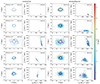 |
Fig. 1. Distribution of the 500 sampled particles of five UMP planar stars in the (X, Y) and (Jϕ, Jz) space, color-coded by their planar radius (R) 6 Gyr ago. The two left columns show that most of the particles approximately maintain their orbits under a constant bar for 6 Gyr. The two right columns show a much larger scatter in both spaces for a decelerating bar. |
We then compare the results from our experiments by showing in Fig. 2 the density plot of all sampled particles in the action space (Jϕ, Jz). The majority of them currently (left panel) reside well within the selection box described in Sect. 2. The middle panel presents the distribution of these particles 6 Gyr ago under a constant bar with spiral arms (model ii) and displays only small changes from their current properties. In the case of a decelerating bar with spiral arms (model iv), shown in the right panel, the distribution of Jϕ is clearly wider and extends below  . The orbits of sampled particles with
  have gained stronger rotation from the bar over the last 6 Gyr. However, their fraction is very small, and the vast majority (92%) of the sampled particles were dominate by rotation (
 ) 6 Gyr ago. The statistical discussions below, are all based on the 284 × 500 particles sampled from the observed values with uncertainties. When we only trace these 284 stars with their observed values, the rotation-dominated percentage is 86%. To roughly estimate the fraction of stars that were in the inner Galaxy with little rotation, we used a cut of
  to select original bulge-like orbits (Binney & Vasiliev 2023b). Only 3% of the sampled particles qualify, and only one out of the 284 stars below the cut qualifies by taking the observed values.
We further investigated the effect of the different models on the individual orbits of the sampled particles. Fig. 3 shows the density contour plot of the change in ( ) space for all particles under a constant bar (left panel) and a decelerating bar (right panel), with the changes in orbital properties defined as those at present with respect to 6 Gyr ago, that is, ΔJ = J(t = 0 Gyr)−J(t = −6 Gyr). First of all, it is clear that spiral arms have little effect on the actions of the particles: the orange contours that correspond to action changes for the models with spiral arms are very similar to those without (blue contours). In the case of a constant bar, the changes in the orbital properties are marginal, with a distribution of ΔJϕ centered on ∼0 km s−1kpc and a dispersion of only ∼70 km s−1kpc (interval between the 16th and 84th percentile of the distribution of ΔJϕ). The dispersion under a decelerating bar is much wider: from −560 km s−1kpc (16th percentile) to 41 km s−1kpc (84th percentile). The majority of the particles lose rotation within the 6 Gyr of the simulation, and only a small fraction of them (19%) gain rotation from interactions with the bar. This effect could be related to the migration of the corotation resonance-trapped regions in the bar (see details in Li et al. 2024). A bar that changes in pattern speed also changes its corotation with time, which causes a much more efficient radial migration than in the case of a constant bar (see e.g., Monari et al. 2016a). The sampled particles are evenly split between those that have positive ΔJz, indicating that they have become kinematically hotter and gained vertical motion as their orbits are perturbed by the bar, and negative ΔJz, indicating that, conversely, they have become kinematically colder and lost vertical motion.
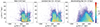 |
Fig. 2. Density plot of all sampled particles in the action space (Jϕ, Jz). Left: Original sample of stars currently in the selection box (black rectangle): 1005 km s−1kpc ≤ Jϕ ≤ 2010 km s−1kpc and 0.175 km s−1kpc ≤ Jz ≤ 437.5 km s−1kpc. Middle: Sampled particles 6 Gyr ago in model (ii) of a constant bar with spiral arms. They remain similar to their initial distribution in the left panel. Right: Particles in model (iv) of a decelerating bar with spiral arms. They have a more extended distribution Jϕ 6 Gyr ago in this model. Some low-Jϕ particles (Jϕ ≲ 1000 km s−1kpc) have gained rotation from the bar, but represent only a small fraction of the entire sample. |
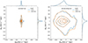 |
Fig. 3. Density contour plot of the action changes with respect to the initial state for all sampled particles. The left and right panels show the case of the constant bar models and the decelerating bar models, respectively. In both panels, the orange contours represent models with spiral arms, and the blue contours show models without spiral arms. Spiral arms only have a small impact on the orbital properties of the particles. The sampled stars under the decelerating bar have a much wider distribution in ΔJϕ and ΔJz compared to those with the constant bar. The majority of the particles lose rotation (ΔJϕ < 0) and only a small fraction of them (19%) have gained rotation from the bar during the last 6 Gyr. |
5. Discussions
We explored the possible origin of the low-metallicity prograde planar stars found in the solar vicinity (heliocentric distances ≲5 kpc) by running orbital integrations backward for 6 Gyr under different bar models. The results show that a rotating bar is no robust mechanism that could explain the existence of these observed stars. First, a constantly rotating bar has little impact on the orbits of the stars. In the extreme case of a decelerating bar, some of these stars can be trapped in the corotation resonance region and be shepherded from the inner Galaxy to the solar neighborhood. However, the majority of the sampled particles (92%) was dominated by rotation (Jϕ ≥ 1000 km s−1kpc) 6 Gyr ago. The chance that they started with low rotation is very low (< 3% with  ). These old prograde planar stars that are currently present in the solar neighborhood may have different origins, as tentatively shown by the initial analysis of their chemical abundances (Dovgal et al. 2024). Most of them started with rotation-dominated orbits after their birth and thus were either born in situ in the proto-MW disk, came from accreted systems that merged onto the MW with very prograde orbits, or were brought in with the clumps that formed the proto-MW (Sestito et al. 2021).
From the modeling aspect, our method is capable of exploring the origins of stars by tracing them under different bar models. However, there are key limitations to this approach. First, the decelerating bar model is only a toy model that cannot represent the true evolution history of the bar in the Galaxy. For example, the pattern speed drops drastically faster than for current values estimated in the Galaxy (Chiba et al. 2021). Second, the test-particle simulation method does not include any response of the stellar systems to the perturbations by the bar and the spiral arms that is due to the self-gravity of the system itself. Third, the method does not take into account the evolution or increase of the background potential of the Galaxy itself over the last 10 Gyr, especially in the epochs between 6 and 10 Gyr ago, and it does not take into account the possibility that recurring spiral arms with resonances at different radii, which also overlap the bar resonances at different radii over time (Sellwood & Binney 2002; Minchev & Famaey 2010), could enhance the migration process of the old stars after the process has started. Future improvements of this method need more explicit knowledge of the evolution history of the bar pattern speed and radial profiles. The toy models presented here are nevertheless useful to explore possible scenarios before proceeding with more complex modeling and simulations.
From the observational side, the strong selection effect of the different ground-based survey samples we used may lead to a misunderstanding of their true distribution. Any quantitative interpretation requires a comprehensive selection function for the data. This will be greatly facilitated by systematic surveys of low-metallicity stars, such as the upcoming WEAVE (Jin et al. 2024) and 4MOST surveys (de Jong et al. 2019). In addition, the ability to detect the very low-metallicity prograde planar stars is still mainly limited to lines of sights away from the disk, toward the Galactic caps, because the search for these stars in the disk regions is hampered by the overwhelming population of more metal-rich stars and by the increasingly high extinction. Future near-infrared astrometric surveys, such as the MOONS survey (Gonzalez et al. 2020) and Gaia NIR (Hobbs et al. 2016), would certainly be a significant improvement, but will require new techniques for identifying the most metal-poor stars that are currently being discovered in photometric surveys using optically blue wavelengths.
Acknowledgments
ZY, NFM, BF, GM, and RAI acknowledge funding from the European Research Council (ERC) under the European Unions Horizon 2020 research and innovation programme (grant agreement No. 834148). CL, AS, BF, GM, VH and GK acknowledge funding from the ANR grant ANR-20-CE31-0004 (MWDisc). ZY, NFM, GK, and VH gratefully acknowledge support from the French National Research Agency (ANR) funded project “Pristine” (ANR-18-CE31-0017). RC thanks support by the the Natural Sciences and Engineering Research Council of Canada (NSERC), [funding reference #DIS-2022-568580]. AAA acknowledges support from the Herchel Smith Fellowship at the University of Cambridge and a Fitzwilliam College research fellowship supported by the Isaac Newton Trust. GT acknowledges support from the Agencia Estatal de Investigación del Ministerio de Ciencia en Innovación (AEI-MICIN) and the European Regional Development Fund (ERDF) under grant number PID2020-118778GB-I00/10.13039/501100011033 and the AEI under grant number CEX2019-000920-S. ES acknowledges funding through VIDI grant “Pushing Galactic Archaeology to its limits” (with project number VI.Vidi.193.093) which is funded by the Dutch Research Council (NWO). This research has been partially funded from a Spinoza award by NWO (SPI 78-411). This research was supported by the International Space Science Institute (ISSI) in Bern, through ISSI International Team project 540 (The Early Milky Way). ZY thanks the discussions with Adam Dillamore and Vasily Belokurov during the MW-Gaia workshop supported by COST Action CA18104: MW-Gaia. This work has made use of data products from the Guo Shou Jing Telescope (LAMOST). LAMOST is a National Major Scientific Project built by the Chinese Academy of Sciences. Funding for the project has been provided by the National Development and Reform Commission. LAMOST is operated and managed by the National Astronomical Observatories, Chinese Academy of Sciences. This work has made use of data from the European Space Agency (ESA) mission Gaia (https://www.cosmos.esa.int/gaia), processed by the Gaia Data Processing and Analysis Consortium (DPAC, https://www.cosmos.esa.int/web/gaia/dpac/consortium). Funding for the DPAC has been provided by national institutions, in particular the institutions participating in the Gaia Multilateral Agreement.
References
- Aguado, D. S., Youakim, K., González Hernández, J. I., et al. 2019, MNRAS, 490, 2241 [NASA ADS] [CrossRef] [Google Scholar]
- Arentsen, A., Starkenburg, E., Martin, N. F., et al. 2020a, MNRAS, 491, L11 [Google Scholar]
- Arentsen, A., Starkenburg, E., Martin, N. F., et al. 2020b, MNRAS, 496, 4964 [NASA ADS] [CrossRef] [Google Scholar]
- Argast, D., Samland, M., Gerhard, O. E., & Thielemann, F. K. 2000, A&A, 356, 873 [Google Scholar]
- Beers, T. C., & Christlieb, N. 2005, ARA&A, 43, 531 [NASA ADS] [CrossRef] [Google Scholar]
- Beers, T. C., Preston, G. W., & Shectman, S. A. 1992, AJ, 103, 1987 [NASA ADS] [CrossRef] [Google Scholar]
- Belokurov, V., & Kravtsov, A. 2022, MNRAS, 514, 689 [NASA ADS] [CrossRef] [Google Scholar]
- Belokurov, V., & Kravtsov, A. 2023, MNRAS, 525, 4456 [NASA ADS] [CrossRef] [Google Scholar]
- Binney, J. 2020, MNRAS, 495, 895 [NASA ADS] [CrossRef] [Google Scholar]
- Binney, J., & Vasiliev, E. 2023a, MNRAS, 520, 1832 [NASA ADS] [CrossRef] [Google Scholar]
- Binney, J., & Vasiliev, E. 2023b, arXiv e-prints [arXiv:2306.11602] [Google Scholar]
- Carollo, D., Christlieb, N., Tissera, P. B., & Sillero, E. 2023, ApJ, 946, 99 [NASA ADS] [CrossRef] [Google Scholar]
- Chiba, R., & Schönrich, R. 2021, MNRAS, 505, 2412 [NASA ADS] [CrossRef] [Google Scholar]
- Chiba, R., & Schönrich, R. 2022, MNRAS, 513, 768 [NASA ADS] [CrossRef] [Google Scholar]
- Chiba, R., Friske, J. K. S., & Schönrich, R. 2021, MNRAS, 500, 4710 [Google Scholar]
- Christlieb, N., Schörck, T., Frebel, A., et al. 2008, A&A, 484, 721 [NASA ADS] [CrossRef] [EDP Sciences] [Google Scholar]
- Cooper, A. P., Koposov, S. E., Allende Prieto, C., et al. 2023, ApJ, 947, 37 [NASA ADS] [CrossRef] [Google Scholar]
- Cox, D. P., & Gómez, G. C. 2002, ApJS, 142, 261 [NASA ADS] [CrossRef] [Google Scholar]
- de Jong, R. S., Agertz, O., Berbel, A. A., et al. 2019, The Messenger, 175, 3 [NASA ADS] [Google Scholar]
- Di Matteo, P., Spite, M., Haywood, M., et al. 2020, A&A, 636, A115 [NASA ADS] [CrossRef] [EDP Sciences] [Google Scholar]
- Dillamore, A. M., Belokurov, V., Evans, N. W., & Davies, E. Y. 2023, MNRAS, 524, 3596 [NASA ADS] [CrossRef] [Google Scholar]
- Dovgal, A., Venn, K. A., Sestito, F., et al. 2024, MNRAS, 527, 7810 [Google Scholar]
- El-Badry, K., Bland-Hawthorn, J., Wetzel, A., et al. 2018, MNRAS, 480, 652 [NASA ADS] [CrossRef] [Google Scholar]
- Frebel, A. 2010, Astron. Nachr., 331, 474 [NASA ADS] [CrossRef] [Google Scholar]
- Gallart, C., Bernard, E. J., Brook, C. B., et al. 2019, Nat. Astron., 3, 932 [NASA ADS] [CrossRef] [Google Scholar]
- Gonzalez, O. A., Mucciarelli, A., Origlia, L., et al. 2020, The Messenger, 180, 18 [NASA ADS] [Google Scholar]
- Green, G. M., Schlafly, E., Zucker, C., Speagle, J. S., & Finkbeiner, D. 2019, ApJ, 887, 93 [NASA ADS] [CrossRef] [Google Scholar]
- Hernitschek, N., Cohen, J. G., Rix, H.-W., et al. 2018, ApJ, 859, 31 [NASA ADS] [CrossRef] [Google Scholar]
- Hobbs, D., Høg, E., Mora, A., et al. 2016, arXiv e-prints [arXiv:1609.07325] [Google Scholar]
- Horta, D., Cunningham, E. C., Sanderson, R., et al. 2024, MNRAS, 527, 9810 [Google Scholar]
- Howes, L. M., Asplund, M., Keller, S. C., et al. 2016, MNRAS, 460, 884 [NASA ADS] [CrossRef] [Google Scholar]
- Jin, S., Trager, S. C., Dalton, G. B., & Aguerri, J. A. L. 2024, MNRAS, 530, 2688 [NASA ADS] [CrossRef] [Google Scholar]
- Katz, D., Sartoretti, P., Guerrier, A., et al. 2023, A&A, 674, A5 [NASA ADS] [CrossRef] [EDP Sciences] [Google Scholar]
- Li, H., Tan, K., & Zhao, G. 2018, ApJS, 238, 16 [CrossRef] [Google Scholar]
- Li, C., Siebert, A., Monari, G., Famaey, B., & Rozier, S. 2023, MNRAS, 524, 6331 [NASA ADS] [CrossRef] [Google Scholar]
- Li, C., Yuan, Z., Monari, G., et al. 2024, A&A, 690, A26 [NASA ADS] [CrossRef] [EDP Sciences] [Google Scholar]
- Lindegren, L., Klioner, S. A., Hernández, J., et al. 2021, A&A, 649, A2 [EDP Sciences] [Google Scholar]
- Martin, N. F., Starkenburg, E., Yuan, Z., et al. 2024, A&A, in press, https://doi.org/10.1051/0004-6361/202347633 [Google Scholar]
- McMillan, P. J. 2017, MNRAS, 465, 76 [NASA ADS] [CrossRef] [Google Scholar]
- Minchev, I., & Famaey, B. 2010, ApJ, 722, 112 [Google Scholar]
- Monari, G., Famaey, B., & Siebert, A. 2016a, MNRAS, 457, 2569 [Google Scholar]
- Monari, G., Famaey, B., Siebert, A., et al. 2016b, MNRAS, 461, 3835 [Google Scholar]
- Rix, H.-W., Chandra, V., Andrae, R., et al. 2022, ApJ, 941, 45 [NASA ADS] [CrossRef] [Google Scholar]
- Sanders, J. L., Kawata, D., Matsunaga, N., et al. 2024, MNRAS, 530, 2972 [NASA ADS] [CrossRef] [Google Scholar]
- Santistevan, I. B., Wetzel, A., Sanderson, R. E., et al. 2021, MNRAS, 505, 921 [NASA ADS] [CrossRef] [Google Scholar]
- Schlegel, D. J., Finkbeiner, D. P., & Davis, M. 1998, ApJ, 500, 525 [Google Scholar]
- Sellwood, J. A., & Binney, J. J. 2002, MNRAS, 336, 785 [Google Scholar]
- Sestito, F., Longeard, N., Martin, N. F., et al. 2019, MNRAS, 484, 2166 [NASA ADS] [CrossRef] [Google Scholar]
- Sestito, F., Martin, N. F., Starkenburg, E., et al. 2020, MNRAS, 497, L7 [Google Scholar]
- Sestito, F., Buck, T., Starkenburg, E., et al. 2021, MNRAS, 500, 3750 [Google Scholar]
- Sormani, M. C., Gerhard, O., Portail, M., Vasiliev, E., & Clarke, J. 2022, MNRAS, 514, L1 [NASA ADS] [CrossRef] [Google Scholar]
- Starkenburg, E., Oman, K. A., Navarro, J. F., et al. 2017, MNRAS, 465, 2212 [NASA ADS] [CrossRef] [Google Scholar]
- Vasiliev, E. 2019, MNRAS, 482, 1525 [Google Scholar]
- Wegg, C., Gerhard, O., & Portail, M. 2015, MNRAS, 450, 4050 [NASA ADS] [CrossRef] [Google Scholar]
- Wolf, C., Onken, C. A., Luvaul, L. C., et al. 2018, PASA, 35, e010 [Google Scholar]
- Wylie, S. M., Clarke, J. P., & Gerhard, O. E. 2022, A&A, 659, A80 [NASA ADS] [CrossRef] [EDP Sciences] [Google Scholar]
- Xiang, M., & Rix, H.-W. 2022, Nature, 603, 599 [NASA ADS] [CrossRef] [Google Scholar]
- Yao, Y., Ji, A. P., Koposov, S. E., & Limberg, G. 2024, MNRAS, 527, 10937 [Google Scholar]
- Yuan, Z., Myeong, G. C., Beers, T. C., et al. 2020, ApJ, 891, 39 [NASA ADS] [CrossRef] [Google Scholar]
All Tables
All Figures
|
Fig. 1. Distribution of the 500 sampled particles of five UMP planar stars in the (X, Y) and (Jϕ, Jz) space, color-coded by their planar radius (R) 6 Gyr ago. The two left columns show that most of the particles approximately maintain their orbits under a constant bar for 6 Gyr. The two right columns show a much larger scatter in both spaces for a decelerating bar. |
| In the text | |
|
Fig. 2. Density plot of all sampled particles in the action space (Jϕ, Jz). Left: Original sample of stars currently in the selection box (black rectangle): 1005 km s−1kpc ≤ Jϕ ≤ 2010 km s−1kpc and 0.175 km s−1kpc ≤ Jz ≤ 437.5 km s−1kpc. Middle: Sampled particles 6 Gyr ago in model (ii) of a constant bar with spiral arms. They remain similar to their initial distribution in the left panel. Right: Particles in model (iv) of a decelerating bar with spiral arms. They have a more extended distribution Jϕ 6 Gyr ago in this model. Some low-Jϕ particles (Jϕ ≲ 1000 km s−1kpc) have gained rotation from the bar, but represent only a small fraction of the entire sample. |
| In the text | |
|
Fig. 3. Density contour plot of the action changes with respect to the initial state for all sampled particles. The left and right panels show the case of the constant bar models and the decelerating bar models, respectively. In both panels, the orange contours represent models with spiral arms, and the blue contours show models without spiral arms. Spiral arms only have a small impact on the orbital properties of the particles. The sampled stars under the decelerating bar have a much wider distribution in ΔJϕ and ΔJz compared to those with the constant bar. The majority of the particles lose rotation (ΔJϕ < 0) and only a small fraction of them (19%) have gained rotation from the bar during the last 6 Gyr. |
| In the text | |
Current usage metrics show cumulative count of Article Views (full-text article views including HTML views, PDF and ePub downloads, according to the available data) and Abstracts Views on Vision4Press platform.
Data correspond to usage on the plateform after 2015. The current usage metrics is available 48-96 hours after online publication and is updated daily on week days.
Initial download of the metrics may take a while.