


| Issue |
A&A
Volume 711, July 2026
|
|
|---|---|---|
| Article Number | A287 | |
| Number of page(s) | 16 | |
| Section | Interstellar and circumstellar matter | |
| DOI | https://doi.org/10.1051/0004-6361/202659670 | |
| Published online | 23 July 2026 | |
Untangling dust emission and cosmic infrared background anisotropies with the scattering transform statistics
1
School for Physical Sciences, National Institute of Science Education and Research,
HBNI Jatni - 752050,
India
2
Homi Bhabha National Institute, Training School Complex,
Anushakti Nagar,
Mumbai
400094,
India
3
Laboratoire de Physique de l’École Normale Supérieure, ENS, Université PSL, CNRS, Sorbonne Université, Université Paris Cité,
75005
Paris,
France
4
Laboratoire d’Océanographie Physique et Spatiale (LOPS),
Univ. Brest, CNRS, Ifremer, IRD,
29200
Brest,
France
★ Corresponding authors: This email address is being protected from spambots. You need JavaScript enabled to view it.
; This email address is being protected from spambots. You need JavaScript enabled to view it.
Received:
2
March
2026
Accepted:
27
May
2026
Abstract
Context. A template-fit approach is often used to separate the Galactic dust emission and the cosmic infrared background (CIB) anisotropies in low H I column density regions using the observational fact that the 21 cm H I line emission from neutral atomic hydrogen and dust are tightly correlated. However, in some regions with molecular hydrogen, diffuse ionised gas, and dark gas, the same approach fails to trace the excess Galactic dust emission.
Aims. We developed and tested a statistical component-separation method to extract the dust signal from the contaminated Planck 353 GHz observations using the scattering covariance (SC) statistics, which is a subclass of scattering transform statistics.
Methods. We first obtained a set CIB maps over 25 square patches, each with a sky area of 222 deg2, using the linear correlation of dust and Galactic H I column density map valid in low H I column density regions using the template-fit approach. We then constructed from these 25 maps a generative model of CIB using SC statistics. We finally relied on this generative model to perform a componentseparation of dust and CIB in the Planck data for different sky regions. These separations were achieved by sampling an ensemble of dust maps through pixel-based optimisation, which, when added to the CIB contamination model, verified all the statistics and cross statistics constraints that were estimated directly from the data.
Results. We validated our algorithm and separated the dust emission from the contamination in the Planck 353 GHz observations. We show the results of the recovered dust map for a test sky region where there is a significant difference between the Planck dust map and CSFD map. We found that the Planck dust map has more structure than the CSFD map. We compared the power spectrum of the recovered dust map and H I map and found a difference in slope (∆α ≈ 0.4) by fitting a power-law model to the two spectra. To explain ∆α, we decomposed the recovered dust map into two gas phases: dust associated with neutral atomic hydrogen, and dust associated with molecular hydrogen. We provide a clear pathway to mapping the Galactic interstellar reddening over intermediate and high Galactic latitudes.
Key words: methods: statistical / dust, extinction / infrared: diffuse background / submillimeter: diffuse background
© The Authors 2026
 Open Access article, published by EDP Sciences, under the terms of the Creative Commons Attribution License (https://creativecommons.org/licenses/by/4.0), which permits unrestricted use, distribution, and reproduction in any medium, provided the original work is properly cited.
This article is published in open access under the Subscribe to Open model. This email address is being protected from spambots. You need JavaScript enabled to view it. to support open access publication.
1 Introduction
The cosmic microwave background (CMB) signal encoding the history of the Universe at microwave and far-infrared frequencies is buried deep below the large-scale emission from the Galaxy and the small-scale emission from the extra-galactic sources (Ichiki 2014). At frequencies above 200 GHz, diffuse thermal emission from our own Galaxy and cosmic infrared background (CIB; Puget et al. 1996; Lagache et al. 2005) are the primary contributors to foreground emission (Planck 2018 results. IV. 2020). Galactic thermal dust emission provides a wealth of information regarding the complex physical systems that form the interstellar medium (ISM) (Draine 2011). The CIB is the diffuse radiation from dust particles in star-forming galaxies through the evolution of the Universe, and it acts as a probe for the dark matter distribution and star formation history (Hauser & Dwek 2001; Planck 2013 results. XXX. 2014; Maniyar, A. S. et al. 2018). Moreover, the CIB plays a vital role in de-lensing the observed CMB B modes (Larsen et al. 2016).
Although they have very different origins, dust emission and the CIB share a similar spectral energy distribution; both follow a modified blackbody spectrum with a slightly different spectral index. Separating these two components is challenging using spectral information alone.
Galactic thermal dust emission was observed to be tightly correlated with the 21 cm H I emission in low H I column density regions (Boulanger et al. 1996; Boulanger & Perault 1988). For this reason, the H I emission map is often used as a tracer of the dust emission within a template-fit approach to separate it from the CIB anisotropies (Planck intermediate results. XVII. 2014; Adak et al. 2024) and study its spectral energy distribution. Several other attempts have been made to obtain a clean map of CIB anisotropies by taking advantage of the full velocity coverage (|vLSR| < 600kms−1) of 21 cm H I observations (Planck early results. XXIV. 2011; Lenz et al. 2019; McCarthy 2024), where vLSR is the velocity of the H I gas measured in the local standard of rest frame. The dust-CIB separation using the template-fit approach, however, becomes challenging when the zero level of the sky background is unknown and there are significant variations in the dust emissivity at high Galactic latitudes. Planck 2013 results. VIII. (2014) used a constant dust emissivity in very low HI column density regions (NHI < 2 × 1020cm−2) to set the zero level of the Planck intensity map at 857 GHz. Planck 857 GHz was then used as a reference to set the zero level of all other Planck high frequency instrument (HFI) intensity maps. More recently, Adak et al. (2024) generalised this approach by fitting a pixel-dependent dust emissivity and a global offset using the Galactic H I template within a Bayesian inference framework. The dust and CIB can be separated at the power spectrum level, where the H I power spectrum is used as a tracer of the dust power spectrum and subtracted from the total map to estimate the CIB power spectrum (Mak et al. 2017; Viero et al. 2019). Another model-independent approach used the generalized needlet internal linear combination method, which employs spatial information of the CIB in terms of its angular power spectrum to disentangle dust emission from CIB anisotropies (Planck intermediate results. XLVIII. 2016).
Another approach to separate dust emission from CIB anisotropies is to rely on scattering transform (ST) statistics. ST statistics are a family of low-variance summary statistics inspired by neural networks that efficiently characterise nonGaussian processes (Bruna & Mallat 2013; Andén & Mallat 2014). ST statistics are constructed from convolutions with a set of pass-band wavelets that separate a signal into its different oriented scales, and non-linear operations, such as modulus, that characterise the interaction, that is, the statistical dependence, between these different scales (Cheng & Ménard 2021). Since their introduction in astrophysics, these statistics have consistently approached or reached the best possible performance in characterising, classifying, and inferring parameters in various domains, such as the interstellar medium (Allys et al. 2019; Regaldo-Saint Blancard et al. 2020; Saydjari et al. 2021; Lei & Clark 2023; Richard et al. 2025), the large-scale structures of the Universe (Allys et al. 2020; Eickenberg et al. 2022; Valogiannis & Dvorkin 2022), weak lensing (Cheng et al. 2020; Cheng & Ménard 2021), and the epoch of reionisation (Greig et al. 2022; Hothi et al. 2024).
Additionally, STs offer the ability to construct an approximate generative model of a given process from an estimate of its ST statistics (Bruna & Mallat 2018). This has been demonstrated for various physical processes, with models sometimes constructed from a single image (Allys et al. 2020; Cheng et al. 2024). Initially developed for two-dimensional (2D) planar data, these models have since been expanded to include multifrequency data (Blancard et al. 2023), spherical data (Mousset et al. 2024; Campeti et al. 2025), and even spectroscopic data (Hothi et al. 2026). Simulated data in CMB studies showed that an ST generative model constructed from a single dustforeground patch can suffice for training a neural network to distinguish primordial B modes from dust emission, even within a challenging mono-frequency approach (Jeffrey et al. 2021).
Moreover, new ST-based component-separation algorithms have been developed. Introduced in Regaldo-Saint Blancard, Bruno et al. (2021); Delouis et al. (2022) to separate Galactic dust emission from instrumental noise in Planck data, these versatile algorithms relied on pixel-space optimisation under ST statistics constraints to generate dust maps compatible with the data once added to the noise. In these papers, the ability of these algorithms to leverage the different non-Gaussian properties of different signals was emphasised by the fact that the separations were performed at a single frequency. Additionally, these separations were performed without assuming a prior model of the component of interest (dust, in this case). Recently, Auclair et al. (2024) used an ST-based algorithm to separate dust emission from CIB anisotropies in Herschel Spectral and Photometric Imaging Receiver (SPIRE) observations. A major success of this paper is that this separation was achieved by relying on observational data alone, first learning an ST-based CIB model from a sky region where this signal was dominant, and then using this model to separate Galactic dust emission and CIB in the Spider region. More recently, Tsouros et al. (2026) used the ST-based component-separation to recover the polarised dust emission from the Planck data at 353 GHz.
The main goal of this paper is to build on previous work and separate the Galactic dust emission in Planck 353 GHz data from the CIB anisotropies and instrumental noise. To do this, we first construct an ST-based contamination model of CIB and instrumental noise over a set of square patches, each with a sky area of 222 deg2, in regions of low H I column density. Secondly, we use this contamination model to perform an ST-based componentseparation in regions of intermediate H I column densities. We use the particular scattering covariance (SC) statistics, a subclass of the ST statistics. We work with Planck 353 GHz data smoothed to an angular beam resolution of 16.2′ (full width at half maximum; FWHM) to match the angular beam resolution of the H I emission maps. At this angular beam resolution, the CIB anisotropies dominate instrumental noise. Before applying the component-separation algorithm to the real Planck data, we successfully test it on the simulated Planck maps with different signal-to-noise (S/N) ratios of the dust emission with respect to the contamination.
The paper is organised as follows. In Sect. 2, we describe the Planck data and the external datasets (HI4PI and dust-reddening map at 100 µm). Section 3 briefly describes the results of the template-fit approach to obtain the contamination map (or dust-subtracted Planck map) at 353 GHz over the low H I column density regions. In Sect. 4, we estimate the statistical properties of the contamination map from a limited set of square patches and its sample variance. In Sect. 5 we briefly present the set of ST statistics. The component-separation algorithm using the ST statistics is described in Sect. 6. In Sect. 7, we apply our algorithm to Planck simulations at 353 GHz. We present and discuss the results of the dust-CIB separation obtained from the Planck 353 GHz observations in Sect. 8, and finally, we summarise our findings in Sect. 9.
2 Datasets
2.1 Planck data
We used the publicly available Planck1 spectral matching independent component analysis (SMICA) CMB-subtracted intensity map from the Public Release 3 at 353 GHz (Planck 2018 results. I. 2020). The 353 GHz map is provided in HEALPix2 (Górski et al. 2005) format at Nside = 2048 (pixel size ~1.7′) with an angular beam resolution of 4.82′ FWHM (Planck 2018 results. III. 2020; Planck 2018 results. IV. 2020). We then smoothed the map at an angular beam resolution of 16.2′ (by convolving it with an additional Gaussian beam of  ) and downgraded it to Nside = 512 (pixel size 6.8′). We converted the map from KCMB to kJy sr−1 units using the conversion factors given in Planck 2013 results. IX. (2014). We retained the CIB monopole that was added by hand to the Planck data at 353 GHz. From the HEALPix map, we extracted 2D tangential projection square patches (256 × 256 pixels) centred around HEALPix pixel of Nside = 4 using the reproject Python package (Robitaille et al. 2020). The pixel size for each square patch was 3.5′, resulting in a total patch area of 222 deg2.
We used the end-to-end full focal plane 10 (FFP10) noise simulations at 353 GHz (Planck 2018 results. III. 2020) to estimate the variance of the instrumental noise in the Planck 353 GHz data. Similar to the Planck data, we first smoothed the noise maps with an additional Gaussian beam smoothing of 15.47′, reprojected them to Nside = 512, and then extracted the 2D patches from them.
2.2 External datasets
We used the HI4PI full-sky map with a spectral resolution of 1.49kms−1, which combines the data from the Effelsberg-Bonn H I Survey (EBHIS; Winkel, B. et al. 2016) and the Galactic AllSky Survey (GASS; McClure-Griffiths et al. 2009; Kalberla et al. 2010). The map is provided on the HEALPix grid at Nside = 1024 (pixel size 3.4′) and a common angular beam resolution of 16.2′ (FWHM). The root mean square brightness temperature uncertainty is 43 mK. Along the optically thin line of sight, the total HI column density (NHI; in units of 1018 cm−2) can be obtained by integrating the brightness temperature (Tb) over the velocity channels using the relation (Dickey & Lockman 1990)
 (1)
(1)
Following Hayakawa & Fukui (2024), we integrated Tb over two velocity ranges of the H I clouds: one range with a low velocity (LV; |vLSR | < 30 km s−1), and the other with an intermediate velocity (IV; 30kms−1 < |vLSR| < 100kms−1). We ignored the high-velocity HI emission (HV; |vLSR| > 90 km s−1) as no significant dust emission is associated with the HV template (Wakker & Boulanger 1986; Planck early results. XXIV. 2011; Lenz et al. 2016; Hayakawa & Fukui 2024). The column densities associated with the LV and IV components are defined as NLV and NIV, respectively. Finally, we downgraded the NLV and NIV maps to the HEALPix grid of Nside = 512 and extracted 2D square patches centred around HEALPix pixel of Nside = 4. We treated the two column density maps as the tracers of the dust emission. We used the sum of the NIV and NLV as a measure of NHI.
The all-sky Galactic dust-reddening map produced by Schlegel, Finkbeiner, & Davis (1998, hereafter SFD) at 100 µm has imprints of extragalactic large-scale structure (LSS) or CIB (Chiang & Ménard 2019). The CIB map at 100 µm (rLSS) was reconstructed by cross-correlating the SFD map with the spectroscopic galaxies and quasars in SDSS. The corrected SFD (CSFD) was produced by subtracting the CIB contamination from the SFD map3 (Chiang 2023). We worked with a publicly available CSFD map and a 100 µm CIB map at a HEALPix resolution of Nside = 512 and smoothed the two maps to a common angular beam resolution of 16.2′ (FWHM). The CSFD map was used as a tracer for the dust emission to produce the Planck simulations.
3 Contamination map from the template-fit approach
In this section, we briefly discuss how we obtained the contamination map (or dust-subtracted Planck map) at 353 GHz.
We used the Adak et al. (2024) formalism to fit the pixeldependent dust emissivity and a global offset over low NH I regions (NHI < 4 × 1020cm−2) using the template-fit approach. We used LV and IV H I templates as a tracer for the dust emission. Because the LV and IV maps are full-sky maps, we easily included the northern and southern Galactic hemispheres in the analysis, and we hence increased the total sky coverage.
We followed the iterative correlation method of Planck intermediate results. XVII. (2014) to construct a global mask, which is defined as follows. Over the initial mask with NHI < 4 × 1020cm−2, we computed the pixel-dependent dust emissivity between the CMB-subtracted Planck intensity map at 353 GHz and the two H I templates, and we then subtracted the best-fit model from the Planck 353 GHz data to produce a residual map. We fit a Gaussian to the residuals, calculated its standard deviation (σG), and removed pixels with absolute values greater than 5σG. We repeated the same procedure until all pixels in the residual map fell within 5σG region of the Gaussian fit to the residuals. We arrived at a converged Galactic mask after five iterations, covering a region of ~13 800 deg2. The total sky fraction covered by the unmasked pixels is fsky = 0.33.
We modelled the input CMB-subtracted Planck intensity data (m) at 353 GHz as the sum of the dust emission (s), CIB anisotropies (c), and the instrumental noise (n),
 (2)
(2)
The global offset of the map (including the CIB monopole) term was included in the signal term s. Using Adak et al. (2024) formalism, we sampled the joint probability distribution of the pixel-dependent dust emissivity and the global offset given the two H I templates and the input data. We modelled s as
 (3)
(3)
where ϵLV and ϵIV correspond to the dust emissivity associated with the LV and IV column density maps, respectively, and O is the global offset. We assumed that the two dust emissivities varied over the sky, but had fixed values within a 1.8° × 1.8° pixel area, corresponding to a single pixel area of a HEALPix Nside = 32 map. The contributions of CIB anisotropies and instrumental noise were propagated through the noise covariance matrix (Adak et al. 2024). The emissivity maps are shown in Fig. A.1. The mean and 1σ standard deviation values of ϵLV and εIV of 2644 Nside = 32 pixels over the northern Galactic hemisphere are 46.5 ± 13.3 and 9.2 ± 41.2kJy sr−1(1020 cm−2)−1, respectively. The mean values of εLV and εIV of 2257 Nside = 32 pixels over the southern Galactic hemisphere are 40.5 ± 10.3 and −17.2 ± 32.7kJy sr−1(1020 cm−2)−1, respectively. We report a global offset value of O = 119.3 ± 0.2kJy sr−1 over the Galactic mask used in our analysis. Our value is very close to the CIB monopole of 130kJy sr−1 added to the Planck map at 353 GHz based on the Béthermin et al. (2010) CIB model. The small difference between our estimate of the global offset and the CIB monopole term added by the Planck collaboration of roughly 10.7 kJy sr−1 (or 37.5 μKCMB) might indicate warm ionized medium associated dust emission at high Galactic latitude (Gaensler et al. 2008), as included in the Planck analysis (Planck 2018 results. XII. 2020).
We refer to the dust map estimated from the template-fit approach within the Bayesian inference framework as sB. Next, we subtracted sB from the input CMB-subtracted map to obtain the residual map, rB = m - sB, which includes the CIB anisotropies, instrumental noise, and possible residual dust emissions (not correlated with the two H I templates). The expected standard deviation of instrumental noise from FFP10 simulations over the Galactic mask is 3.3 kJy sr−1, whereas the expected standard deviation of the CIB anisotropies based on the Planck 2013 best-fit CIB model (Planck 2013 results. XXX. 2014) is 9.3 kJy sr−1. Because the standard deviation of two uncorrelated components is added in quadrature, we safely assumed that rB map is dominated by the CIB anisotropies. The residual map at 353 GHz over the Galactic mask is shown in Fig. 1 in orthographic projection. With the two-template fit, we were able to extract the H I-correlated dust model map and the residual map over roughly twice the sky fraction as compared to the one-template fit analysis in the southern Galactic cap region (Adak et al. 2024). In both cases, the one-dimensional probability distribution of the residuals closely follows the Gaussian distribution. We computed the width of the Gaussian fit (wrB) to the residuals over the common mask generated from the union of our iterative mask and southern Galactic cap region (Adak et al. 2024). We report a marginally smaller width in our analysis (wrB = 9.6 kJy sr−1) as compared to the one-template fit analysis (wrB = 9.9 kJy sr−1), indicating less leakage of Galactic emission in the residual map.
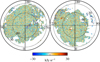 |
Fig. 1 Orthographic projection of the residual map obtained from the template-fit approach. The northern (southern) Galactic hemisphere is shown on the left (right). The white regions are masked from the analysis as they comprise NHI cut-off pixels and the pixels were masked due to iterative masking. |
4 Statistical properties of the residual map over square patches
For our purpose, we first extracted 48 square patches (24 in the northern and 24 in the southern Galactic hemisphere) of size 14.9° × 14.9° (sky area of 222 deg2) centred around the centre of Nside = 4 HEALPix grid pixels at high Galactic latitudes (|b| > 45°). The pixel resolution of each square patch was 3.5′ and contained 256 × 256 pixels. We note that Nside = 4 pixels have a pixel size of 14.7° × 14.7°. All the square patches have very minimal overlap, and they hence provide an independent measurement of the statistical properties of the residual map at 353 GHz. We selected only 25 of these 48 square patches that were not severely affected by the initial mask to select the low NHI regions and the pixels that were masked due to the iterative masking algorithm discussed in Sect. 3. Seventeen of these 25 square patches are completely unaffected by the final mask. Only a few pixels in the remaining 8 square patches are slightly affected by the final mask. The percentage of these masked pixels in these patches is lower than 1.5%. For these 25 square patches, the S/N defined as σ/σ varies from 1 to 2.9.
As the template-fit approach was performed over an area of 1.8° × 1.8° pixels, we expect some leakage of the Galactic dust emission from either the localised Galactic sources present in the Planck map below the 1.8° scale or the dust emission associated with molecular hydrogen (H2) gas or ionised hydrogen (H II) into the residual map. To avoid Galactic residuals in the clean sky patches, we further applied a threshold mask to the 25 square patches. We excluded the pixels lying on the nonGaussian tail part of the one-dimensional probability distribution function of rB map by placing a threshold at ±3σrB. The percentage of the pixels that were masked due to the threshold mask ranges between 0.3% and 0.8%. We inpainted the masked pixels using linear interpolation with griddata function from scipy.interpolate package (Virtanen et al. 2020). Finally, the inpainted patches had no pixels that deviated by ±3σrB, which removed pixels containing contamination by the Galactic residuals. Figure 2 presents all the patches after inpainting was used to derive the statistical properties of the residual map. All the patches follow a Gaussian distribution with a mean standard deviation (σrB) of 8.9 kJy sr−1. The estimated standard deviation of σrB from these patches is 0.4 kJy sr−1, which is much smaller than its mean value. We computed the power spectrum (Cℓ) in these patches using the discrete Fourier transform in the flat-sky approximation (Hivon et al. 2002), implemented in the publicly available package NaMaster4 (Alonso et al. 2019). As these patches do not obey periodic boundary conditions, we masked the boundary pixels in the computation of the power spectrum. We first made a binary mask considering only 180 × 180 inner pixels, as shown in the left panel of Fig. B.1. We then tapered the boundary with a cosine function to create the apodised mask (see the right panel of Fig. B.1). The errors on the power spectrum were computed from the analytic Gaussian covariance matrix using NaMaster. We corrected the final power spectrum for the beam effect and the pixel window effect.
The average power spectrum of these patches is shown in Fig. 3. The sample variance of the power spectrum between all the patches agrees well for the spectra and is broadly consistent with the Lenz et al. (2019) best-fit CIB model (shown with a solid black line). At higher multipoles l > 100, our measurements of the average power spectrum of the residuals and the Lenz et al. (2019) CIB model match very well. We show the average power spectrum up to lmax = 700 because the higher multipoles are significantly affected by the beam correction.
We computed the Minkowski functionals (MFs) for these patches. The MFs provide insight into the geometrical and topological structures of these regions as a variation in the pixel threshold value. For a 2D square patch, the MFs are the area (V0), perimeter (V1), and the Euler characteristic of the connected pixels and the number of holes in the same space or genus (V2). We used the publicly available package QuantImPy (Mantz et al. 2008; Boelens & Tchelepi 2021) to compute the MFs in these regions. Figure 4 shows the MFs of all the 25 selected square patches. We used the best-fit CIB model by Lenz et al. (2019) to generate ten Gaussian realisations of the CIB map and add ten non-Gaussian FFP10 noise realisations to it for a given patch. The solid black line in Fig. 4 shows the MFs obtained from the average of these ten noise-contaminated CIB realisations. As the instrumental noise is subdominant at the beam resolution we chose in our analysis, we conclude that the MFs of the 25 selected square patches closely follow the expected distribution from a Gaussian random field.
 |
Fig. 2 Spatial distribution of the residual maps in the selected 25 square patches. |
 |
Fig. 3 Average power spectrum, in terms of ℓCℓ with multipole ℓ over all the 25 selected square patches (black points). The error bars on them are the standard deviation obtained on the spectra. The solid black line represents the best-fit CIB model by Lenz et al. (2019) at 353 GHz. |
5 Scattering covariance statistics
We used the SC statistics introduced in Cheng et al. (2024) and Mousset et al. (2024). The SC statistics correspond to the covariances of terms constructed from a combination of convolutions of the input random field X with a set of pre-calculated wavelets and a non-linear modulus. The complex valued Mor-let wavelet filters that we used, noted ψj,γ, are localised in pixel and harmonic space, and are characterised by a dyadic scale j ∈ [0, Jmax - 1] and an orientation γ ∈ [0, L - 1]. The wavelets probe characteristic scales of approximately 2j pixels, and are oriented at an angle πγ/L from the reference axis. Jmax < log2(N) is the number of dyadic scales available for a given image of N × N pixels. There are four types of SC statistics. The first S1 and S2 statistics jointly characterise the amplitude and sparsity of the process X at a single oriented scale λ = (j, γ).
The higher-order wavelet moment estimators (S3 and S4) capture the interactions between two and three different oriented scales.
Auto and cross-ST statistics can be computed between two random fields X and Y. The cross SC statistics are defined as
 (4)
(4)
where the asterisk stands for a convolution, the overbar is the complex conjugate, 〈·〉 is the spatial average over the fields, and Cov(X, Y) is the estimated covariances of X and Y. For auto-SC statistics, S1 and S2 are simplified to
 (5)
(5)
while S3 and S4 were obtained by setting X = Y in the previous equations, and the redundant S3p terms was removed. Following previous work (Cheng et al. 2024; Mousset et al. 2024; Campeti et al. 2025), we normalised the  and
and  coefficients by their own
  statistics,
 (6)
(6)
As we worked with fields with 256 × 256 pixels, we set Jmax = 5 and L = 4 for the wavelet filters using the kernel size of 5 × 5 pixels. With these values of Jmax and L, we obtained 2522 auto statistics and 2762 cross statistics. At the end, the final summary statistics Φ that we used for the cross statistics were the concatenation of the mean of the fields 〈XY〉, its variance Var(XY), and the normalised cross SC statistics, as
 (7)
(7)
For the auto statistics, the final summary statistics Φ were the concatenation of the mean of the field 〈X〉, its variance Var(X), and the normalised SC statistics, yielding
 (9)
(9)
We computed these summary statistics using the Python package Foscat5 (Delouis et al. 2022; Campeti et al. 2025).
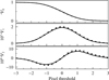 |
Fig. 4 Variation in V0, V1, and V2 with the pixel threshold of the MFs over all the 25 patches. The perimeter and Euler functions are scaled with 102 and 104, respectively, for visualisation purpose. The solid black line represents the MFs computed from the average of ten FFP10 noise-contaminated Gaussian CIB realisations over a given patch. |
6 Component-separation algorithm
In this section, we present the component-separation algorithm based on SC statistics to statistically separate the dust emission from the contamination at 353 GHz Planck observations.
6.1 Generative contamination maps
We generated 300 synthetic contamination maps (rsyn) from the 25 selected patches obtained in Sect. 4. These synthetic maps were constructed using maximum entropy generative models conditioned by the Φ statistics, as defined in Eq. (8) (we refer to Bruna & Mallat 2018; Cheng et al. 2024; Mousset et al. 2024 for more details).
We discuss below the steps that we followed to generate one of synthetic contamination maps. Starting from a white-noise realisation u0, we performed a gradient descent in pixel space to minimise the following6 loss function:
 (9)
(9)
where ∥·∥ is the Euclidean norm, and rB is one of the residual patch. The samples of the generative models are the maps rsyn,i obtained at the end of the optimisation, which verify
 (10)
(10)
We optimised the loss function using the gradient descent algorithm in pixel space implemented in the Foscat package. The optimisation stopped when the difference of the loss functions in the two consecutive iterations was smaller than 10−6.
6.2 Component-separation algorithm
We started with the data map m that we aimed to separate into the dust emission and the contamination. This was done by constructing maps that verified an ensemble of constraints that were constructed directly from the available data. The formalism for this statistical component-separation closely follows the formalisms presented in Delouis et al. (2022) and Auclair et al. (2024). We used six constraints to recover a dust map that was statistically compatible with the information available in the Planck data. The algorithm relies on a gradient descent on a running u map, which at the end of the optimisation corresponds to the recovered s map of the dust emission. We write below the constraints that this s map should fulfill, before expressing these constraints as losses involving the running u map. The first constraint ensures that the recovered signal added to the contamination statistically matches the data. In terms of the summary statistics, the constraint is written as
 (11)
(11)
where 〈·〉 is the ensemble average over the N rsyn maps obtained in Sect. 6.1. The second constraint imposes that the crosscorrelation between the data and the signal is conserved,
 (12)
(12)
The third constraint imposes that the statistics of the residual map r̃ = (m - s̃) matches those of the rsyn. This constraint ensures minimum leakage of the contamination into the recovered dust map. Mathematically,
 (13)
(13)
The fourth constraint enforces that the recovered dust map retains the same correlation with the total NH I map as present in the data. The assumption here is that the contamination maps, being independent from the total NH I, can be sampled again without modifying the estimate of the cross statistics. Mathematically, it is written as
 (14)
(14)
The fifth constraint is that the residual map is uncorrelated with the NH I map, which yields
 (15)
(15)
Finally, the sixth constraint imposes that the residual map is uncorrelated with the dust map separately,
 (16)
(16)
The last four constraints enforce minimum leakage of the dust signal into the contamination map at the angular scales at which the amplitude of the dust signal is comparable to that of the contamination.
Following Delouis et al. (2022), the mathematical loss functions corresponding to these constraints are respectively written as
 (17)
(17)
We minimised the total loss function, given as
 (18)
(18)
For the detailed concept behind the bias B and standard deviation σ, we refer to Delouis et al. (2022). For example, the loss L1 is computed as the normalised chi-square distribution between Φ(m) and  . However, for computational efficiency, it relies on an bias B1, which is estimated only after a certain number of iterations. This avoids the need to trace
  throughout the optimisation. This bias is only necessary when the loss involves an ensemble average over the rsyn,i maps.
The different initial condition maps for the gradient descent were made from the m map smoothed with a W′ (FWHM) Gaussian beam, where W was chosen randomly from a uniform distribution U[100,200]. Starting from the initial map u0, we minimised the total loss function using the gradient descent algorithm in Foscat. The final dust map s̃ corresponded to u at the end of the optimisation, and the residual map was obtained as r̃ = (m - s̃). In practice, we updated the B1, B2 and B4 biases and all variance terms every 150 iterations. We ran this optimisation until the difference between two consecutive losses in an epoch was ΔL < 0.002. The typical number of epochs required to reach the ΔL varied from five to eight, depending on the data map. Numerically, we found that decreasing ΔL beyond 0.002 did not improve the recovered dust map. The total computation time ranged from 15 to 20 minutes on a single-node GPU cluster (NVIDIA A30), depending on the number of iterations performed.
Planck simulations
We first validated the component-separation algorithm described in Sect. 6.2 on simulated Planck maps on a 2D square patch.
7.1 Synthetic contamination maps
We synthesised 12 statistically identical realisations from each sky patch considered in Sect. 3, totaling N = 300 realisations of rsyn maps using the summary statistics, as discussed in Sect. 6.1. The synthetic contamination maps retained the all the statistical properties of the rB and had a mean standard deviation σrsyn of 9.0kJy sr−1, and the estimated 1σ variation in the σrsyn was 0.4k Jy sr−1. These synthetic maps followed the Gaussian distribution and had the same one-dimensional probability distribution function as the rB maps. We also computed the angular power spectra and the three MFs. They followed the mean rB statistics. For brevity, we only show the mean and standard deviation of the S1 and S2 coefficients obtained from the 25 rB and 300 rsyn maps in Fig. 5. We show the mean and standard deviation of the other two normalised coefficients S̄3 and S̄4 in Fig. C.1. We used these 300 rsyn maps to compute the variance on its summary statistics.
7.2 Simulated map at 353 GHz
We chose a test patch centred at Galactic coordinates ( l, b ) = (45.0°, −54.3°) of sky area 222deg2. The mean HI column density over the entire patch was 〈NHI〉 = 3.3 × 1020 cm−2. We extracted the same sky patch from the CSFD map and scaled it with a constant factor to produce an input dust map. We kept the contamination map fixed and varied the dust amplitude to produce different S/N maps. The constant scaling factor controls the S/Ns of the input dust map with respect to the contamination.
We validated our algorithm for S/Ns 3 to 9. We discuss the S/N = 3 results in detail and highlight the primary differences among the others. We call the scaled 2D input dust map ssim, to which we added a realisation of the contamination map (rsim) from the generative model rsyn obtained in Sect. 7.1 to produce the contaminated map (msim = ssim + rsim). The Pearson correlation coefficient ρ of ssim with the NHI map for S/N = 3 is 0.94 and was reduced to 0.88 after we added the contamination map rsim. The top panel of Fig. 6 shows the input dust map at S/N = 3, one random realisation of the contamination, and the total contaminated simulated map. msim map is patchy owing to contamination.
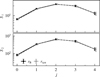 |
Fig. 5 Comparison of the S1 and S2 statistics of mean and standard deviation of 25 contamination maps obtained from the template-fit approach rB regions (black circles) and 300 synthetic contamination maps rsyn (grey crosses). The grey crosses are shifted in the x-axis. |
7.3 Validating the component-separation algorithm
We applied the component-separation algorithm described in Sect. 6.2 to the contaminated map to extract a statistical realisation of the dust signal. By performing the component-separation under different initial conditions, we obtained 25 recovered dust maps. The bottom panel of Fig. 6 shows one of the recovered dust maps (s̃sim), the residual map (r̃sim = msim - s̃sim), and the difference between the input and recovered dust (δs = s̃sim - ssim). We clearly see some Galactic residuals near the boundaries of r̃sim map. To avoid these boundary pixels, we restricted our analysis to the unmasked pixels within the binary mask (shown in the left panel of Fig. B.1) to compute the Pearson correlation coefficients. The value of ρ between ssim and s̃sim was found to be 0.97, showing a tight pixel-to-pixel correlation between the input and recovered dust maps. Visually, the small-scale features dominated by contamination are well separated from the large-scale dust emission. The δs map has no visible large-scale features at the map level. The correlation coefficient ρ = 0.91 between ssim and NH I is the same as was obtained between ssim and NH I. This shows that the component-separation algorithm removes most of the contamination from the total map. The top panel of Fig. 7 shows the auto spectra ℓCℓ of rsim, r̃sim, and δs, along with the magnitude of the cross-spectrum of rsim with δs. The bottom panel presents the cross-spectra ℓ2Cℓ of δs and r̃sim with the NHI map. We applied the apodised mask (Fig. B.1, right) to account for non-periodic boundaries. The power spectrum of the rsim follows an Cℓ ∝ ℓ−1.3 spectrum, which is consistent with the CIB model of Planck 2013 results. XXX. (2014). As our componentseparation algorithm is a statistical method, the δs map captures the phase mismatch between the input and the output dust maps. The δs map is not correlated with NH I map, as is captured by the cross-power spectrum of δs and NH I. The average δs map obtained from 25 realisations is shown in Fig. 8 (third column, top panel). The average δs map is also statistically uncorrelated with NH I at the pixel level (bottom panel of Fig. 8). We show the comparison between the input and output dust spectra in Fig. C.2.
Next, we calculated the SC statistics (S1, S2, S̄3, and S̄4) of these maps. The mean and standard deviation of S1 and S2 for five different j values and four different γ values, computed from 25 recovered dust maps, are shown in Fig. 9. The x-axis represents λ ≡ (j, γ), where λ = 0 corresponds to the smallest scale (j = 0) and the first wavelet orientation. Our component-separation algorithm accurately recovers these statistical properties of the dust map as a function of wavelet scales and orientations. The contamination in msim leads to higher S1 and S2 at small scales (or low j values) compared to ssim. The algorithm recovers almost all the scales of ssim, except for the smallest scales at S/N = 3. We show the remaining two SC statistics S̄3 and S̄4 in Fig. C.3. At S/N ≥ 5, the algorithm recovers S1 and S2 statistics for large and small scales. In Fig. C.4 we present the SC statistics for S/N = 5. The smallest scale (j = 0) between the input and output for all statistics agrees well. Figure 10 shows the angle-averaged S1 and S2 statistics of rsim and r̃sim for different values of j. As the contamination maps is statistically isotropic, there is no preferred orientation at which we expect to see more power. For rsim, we computed the 1σ standard deviation from 300 rsyn maps. In the same plot, we also show the same angle-averaged S1 and S2 cross statistics of the δs and r̃sim maps. The cross S1 and S2 statistics between rsim and r̃sim broadly follow the same statistics as rsim. This means that the r̃sim map retains the phase information of the input rsim up to a certain percentage. Even though δs visually appears to be similar to rsim, the S2 amplitude of δs × r̃sim is much smaller than the corresponding amplitude of rsim × rsim (or r̃sim × r̃sim) at small scales corresponding to low j values. The 1σ deviation on the auto and cross statistics with the recovered maps was computed from the 25 realisations of r̃. Figure 11 shows the angle-averaged cross statistics S2 between r̃sim and NHI map. The error bar on S2 was computed from 25 realisations of the r̃sim, starting from different initial conditions. For completeness, we computed the expected cross statistics S2 between rsyn and NHI map. The mean value of the S2 statistics computed from 300 rsyn maps is consistent with zero, and the 1σ error bars capture patch-to-patch variations of the same statistics. Since we added a single realisation of the contamination to the input dust map, the error bar on the rsim × NHI cross statistics S2 only includes the statistical noise from the component-separation algorithm.
In Fig. 12, we plot the 2D histogram highlighting the joint distribution of ssim and NHI, considering only the pixels those falls within the binary mask. This shows that the ssim has a significant amount of scatter with NHI over the entire patch, and the correlation between them becomes non-linear above NHI > 4 × 1020cm−2. Next, we binned the data into seven bins in order of increasing values of NHI and computed the median values of msim, ssim, and s̃sim over each bin. The upper and lower limit of the error bars at each bin correspond to the 16 and 84 percentile of the three quantities msim, ssim, and s̃sim. This plot shows that the distributions are very similar for these different maps, although there appears to be a consistent reduction in the standard deviation of the distribution at fixed NHI values from msim to s̃sim. This effect is more pronounced in low NHI regions, in which the contamination is comparable to the dust signal. The reduction of the error bars from msim to s̃sim is consistent with the expected outcome of removing contaminants.
Next, we varied the S/N of the dust signal with respect to contamination. For each S/N, we quantified the reliability of the component-separation algorithm. For S/N 3, we demonstrate that our component-separation algorithm successfully and efficiently separates the dust signal from the contamination at the level of summary statistics. The algorithm only recovers the dust signal at large scales for low S/Ns (S/N ≃ 1), leaving excess power at small scales in the recovered dust map. We applied the same procedure to other sky regions for different S/Ns and reached the same conclusions.
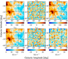 |
Fig. 6 Top : input maps at S/N = 3 centred around the sky patch at (l, b) = (45.0°, −54.3°). The columns from left to right show the input dust map (ssim), the input contamination map (rsim), and the total simulated map (msim). Bottom : columns from left to right: Component-separated dust map (s̃sim), residual map (r̃sim), and difference between input and recovered dust map (δs). |
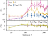 |
Fig. 7 Top : ℓCℓ spectra for rsim (solid pink), r̃sim (dashed red), δs (dashed-dotted orange), and magnitude of the cross-spectrum for rsim and δs (dashed-dot-dotted blue) in kJy2sr−1. Bottom : cross-spectra (l2Cl) of δs (solid green) and r̃sim (dashed brown) with the NHI map, in kJy sr−1(1020cm−2). |
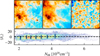 |
Fig. 8 Top : s̃sim (left), HI column density map (middle), and the mean of 25 realisations of δs (right). Bottom : 2D correlation between NHI and 〈δs〉. The blue crosses and the error bars show the median values and standard deviations of mean 〈δs〉 in the ordered bins of NHI. |
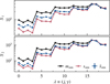 |
Fig. 9 Comparison of S1 and S2 statistics of msim (black circles), ssim (red circles), and the s̃sim (blue crosses with dashed line). |
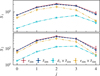 |
Fig. 10 Comparison of the angle-averaged S1 and S2 statistics of rsim (red circles) and r̃sim (blue crosses with the dashed line). The cyan squares with the dashed-dotted line show the cross coefficients between δs and r̃sim, and the orange diamonds with the dashed-dot-dotted line show that between rsim and r̃sim. |
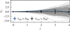 |
Fig. 11 Comparison of the angle-averaged S2 cross statistics with the NHI map: r̃sim (dashed blue) and the mean over 300 rsyn (black). The recovered contamination is consistent with the expected statistics within 1σ. The blue crosses are slightly shifted along the x-axis. The grey lines show all 300 rsyn realisations. |
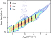 |
Fig. 12 2D histogram showing the joint distribution of ssim and NHI. The black circles correspond to the median values, and the upper and lower limits correspond to the 16 and 84 percentile of msim of the data in each ordered bin of NHI. Similarly, the red circles show ssim, and the blue crosses show s̃sim. |
8 Application to Planck data
8.1 Component-separated maps and its summary statistics
In this section, we primarily focus on the component-separation results on a sky patch of 222 deg2 area centred at Galactic coordinates (l, b) = (247.5°, 66.4°) for brevity. We first subtracted the global offset term of 119.3 kJy sr−1 as obtained from the template-fit approach (see Sect. 3) from the CMB-subtracted Planck data to focus on the statistical separation of the dust emission and CIB contamination using the SC-based statistics. We refer to this map as md. The mean H I column density measured across the entire map is 〈NHI〉 = 2.3 × 1020cm−2. The Pearson correlation coefficient ρ between the md and NHI maps is 0.84.
We applied the component-separation algorithm to extract a statistical realisation of the dust signal. We followed the same steps as described in Sect. 7 and obtained 25 different realisations of dust map. The top panel of Fig. 13 shows the input map (md), recovered residual map (r̃) and a single realisation of the dust map (s̃). The recovered dust map retains most of the large-scale features present in the Planck data and filters out the small-scale fluctuations from the contamination. The mean dust emissivity over the entire sky patch was computed as the mean of the ratio of the recovered dust over NHI, defined as  . The mean value of the dust emissivity is 45 kJy sr−1(1020 cm−2), which is consistent with the value obtained by Planck early results. XXIV. (2011); Planck intermediate results. XVII. (2014), and Adak et al. (2024).
Next, we present the statistics of the residual map (r̃). The top panel in Fig. 14 shows the joint distribution of r̃ and the NHI map. The blue data points are the median values, and the error bars correspond to 1σ standard deviation in seven bins ordered in increasing values of NHI. The median values are consistent with zero, showing no significant leakage of s̃ into the residual map. The plot also confirms that our SC statistics-based componentseparation algorithm works well for the S/N ≈ 8.4 region. The standard deviation of σr̃ over the masked region is 8.1 kJy sr−1, which is consistent with the expected value from 300 rsyn maps. In the middle panel of Fig. 14, we show the S2 comparison of the r̃ map in the Planck field and the expected distribution from 300 rsyn maps. The amplitudes of the S2 statistics match well at low j values, except at the very large scale (j = 4). The difference in S2 statistics between the r̃ and 300 rsyn map is at the level of 2.3σ for j = 4. We also compared the rLSS map at 100 μm from Chiang (2023) at that field. We multiplied the rLSS map (in kJy sr−1 units) by a factor of 0.3 and computed the S2 coefficient. We found that small-scale powers are missing from the rLSS map, but the intermediate and large scales are consistent within the error bands from the synthetic maps. We correlated the s̃ map with r̃ map and found a cross-correlation coefficient ρ = −0.06 between the two maps. We show the cross S2 statistics of s̃ and r̃ in the bottom panel of Fig. 14 to ensure that the recovered maps are statistically uncorrelated at the level of S2 statistics. The 1σ deviations on the coefficients were computed from the cross S2 statistics of s̃ and the 300 rsyn maps. We also computed the cross statistics S2 between the s̃ and rLSS map for the same sky patch. The 1σ deviations on S2 were computed from the cross statistics of s̃ with 94 independent sky patches with a size of 14.9° × 14.9° of the Chiang (2023) CIB/LSS map. All the scales are consistent with the zero within the 1σ error bar, except for the j = 2 scale, where the deviation is at the level of 3.2σ. The cross-correlation coefficient of the s̃ map with rLSS map is ρ = 0.03.
We also performed a non-Gaussianity test to check for any significant leakage of the Galactic residuals into the r map. The results of the non-Gaussianity test are presented in Appendix D. Additionally, we compared the statistics of the contamination maps from two different component-separation algorithms: the template-fit approach, and the SC-based statistics. In Appendix E, we present the component-separation results for the same Planck field as used to validate the component-separation algorithm in Sect. 7.
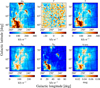 |
Fig. 13 Top : Planck 353 GHz map (CMB and global offset subtracted; left), r̃ (middle) and s̃ (right) after component-separation in the same sky region as in Fig. 6. Bottom : decomposed s̃HI (left) and s̃H2 maps (middle). The sCSFD map at 100 μm (in mag units) in the same sky region is shown in the right panel. |
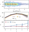 |
Fig. 14 Top : correlation plot of r̃ with NHI map. The blue data points and the error bars show the zero median and standard deviation of r̃ in the ordered bins of NHI. The standard deviations are consistent in all the NHI bins. Middle : comparison of angle-averaged S2 statistics of r̃ (red cross), rLSS (square dashed orange line) and the ensemble average of 300 rsyn maps (black circles) along with 1σ, 2σ, and 3σ error bands. Bottom : red crosses with the solid line show cross S2 coefficients between s̃ and r̃, and the blue circles with the dashed line show the cross S2 coefficients between s̃ and rLSS. The blue circles are slightly shifted in the x-axis. |
8.2 Separation in HI and H2 emission
To understand the morphology of the recovered dust emission, we decomposed it into two components: dust associated with NHI (s̃HI), and dust associated with NH2 (s̃H2),
 (19)
(19)
where s̃HI = εHI,353NHI, and εHI,353 is the dust emissivity of the H I-correlated dust emission at 353 GHz. In our case, εHI,353 is a constant value over the selected sky patch. We estimated the mean 〈εNHI,353〉 from the square patches, defined in Sect. 4, at high Galactic latitudes. We applied the final iterative mask (discussed in Sect. 3) to the high-latitude square patches to select only the low NH I pixels where the dust–H I correlation holds. We also avoided square patches where more than 30% pixels were masked. Finally, we had 40 such high-latitude square patches with a sufficient number of valid pixels for the correlation analysis. Using a simple linear regression with the NH I map, we found a value of the emissivity per square patch. While performing linear regression, we took the standard deviation of the contamination as an error bar per pixel into account. By analysing 40 sky patches, we obtained the mean and standard deviation of the dust emissivity as 〈εH I,353〉 = 38 ± 6kJysr−1 (1020cm−2). We produced 25 realisations of the s̃HI maps by varying εHI,353 within the mean and standard deviation of this estimate. The bottom panel of Fig. 13 shows the decomposition of s̃ in terms of the s̃HI (left panel) and s̃H2 (middle panel) using the value of 〈εHI,353〉. Visually, the s̃H2 map is clumpy, whereas the s̃HI map is more diffuse.
We computed the SC statistics of the s̃HI and s̃H2 maps to characterise their morphological differences. We used the S1 and S2 statistics and the S21/S2 ratio to measure sparsity (Lei et al. 2025). Figure 15 shows the variation in S1, S2, and S12/S2 as a function of λ ≡ (j, γ). The error bars on the SC statistics of the s̃H2 map were computed from the 25 realisations of s̃H2 maps. The first-order coefficient S1 and wavelet power spectrum S2 show that the s̃H I map has more power at large angular scales and at all orientations than the s̃H2 map. The lower values of the ratio S12/S2 for s̃H2 compared to the s̃HI map shows that s̃H2 map is significantly sparser than s̃HI, as the ratio decreases with increasing sparsity of the field. This is consistent with Fig. 13, where the localised high column density structures are only present in the s̃H2 map.
Next, we computed the power spectrum of s̃ and compared it with the power spectrum of NHI. Because of the limited sky coverage of the sky patch, the largest scale we obtained is ℓ ≃ 25. We fitted them with a power-law model, Cℓ ∞ (ℓ/75)α, in the multipole range 25 ≤ ℓ ≤ 625 and found the best-fit value of the exponents as αs̃ = −2.51 ±0.07 and αH I = −2.92±0.10. The difference in the slope of s̃ and NH I spectrum,  , also indicates a significant amount of dust emission associated with gas in the form of H2 (Desert et al. 1988; Reach et al. 1998).
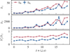 |
Fig. 15 S1, S2, and S21/S2 for the s̃HI map (red circles) and the |

8.3 Comparison of our dust map with the CSFD extinction map
In this section, we compare the recovered Planck dust map at 353 GHz with the CSFD map at 100 μm over the same sky patch as discussed in Sect. 8.1. The right column of Fig. 13 shows the map-level comparison between s (expressed in units of kJy sr−1) and sCSFD (expressed in units of mag). Our first observation is that the Planck dust map contains more localised structures than the CSFD map. This finding is supported by the power spectrum comparison between the two maps. We computed the power spectrum of s̃ and sCSFD over the apodised mask and fitted it with a power-law model within the multipole range 25 ≤ ℓ ≤ 625. The power spectrum exponent for the Planck dust map is αs̃ = −2.51 ± 0.07 and that for the CSFD map is αsCSFD = −2.65 ± 0.09.
Next, we computed the non-linear dependence of s̃ and sCSFD on the NHI map by fitting a power-law model, (s̃, sCSFD) ∝ 〈NHI〉p. The power-law exponent p is expected to be close to 1 in case of a tight correlation between dust and atomic gas. For each of the two dust maps, we grouped the pixel values into seven bins in ascending order of NHI and computed the median values within each NH I bin, as well as the 16 and 84 percentiles, which we used as error bars. We fitted the median values s̃ and sCSFD with the mean NH I (taking the error bars into account) and found that the value of the exponent p is 1.04 for the Planck map and 0.85 for the CSFD map. This result shows that the slope of the power law differs significantly between the Planck and CSFD maps. Furthermore, the data scatter in the NHI correlation is greater for s̃ than for the sCSFD map.
The morphological differences between the recovered Planck dust map and CSFD map can be explained by the different spectral energy distribution (SED) of H I-correlated dust emission and H2-correlated dust emission. When the two SEDs follow the modified black-body spectrum (MBB), then the ratio of the emissivities of the H I and H2-correlated dust components at 353 GHz can be written as
 (20)
(20)
where ν0 = 100 μm is the reference frequency, and B353(T) is the Planck black-body function at 353 GHz. Here, (THI,βH I) and (TH2,βH2) are the temperatures and spectral indices of the HI and H2 -associated dust emission, respectively. We assumed that the ratio  . When we neglected the attenuation of the interstellar radiation field by dust within the diffuse interstellar medium, the integral of the MBB spectrum or the dust radiance (given by Eq. (10) in Planck 2013 results. XI. 2014) did not vary from H I to the H2 gas. Under these two assumptions, the constraint relation between the SED parameters of H I and H2-associated dust emission is
 (21)
(21)
We adopted THI = 20 K and βHI = 1.65 from Planck intermediate results. XVII. (2014), computed from the MBB fit to the dust emissivities at the far-infrared frequencies 353, 545, and 857 GHz and COBE-DIRBE 100 µm for the H I-correlated dust emission. The change in βH2 follows from that of TH2, and thus, the change in relative grain emissivity at 353 GHz. We fitted the sCSFD map with two templates (s̃HI and s̃H2) and a constant offset (O) over the valid pixels within the binary mask. We modelled the sCSFD map as
 (22)
(22)
The best-fit values of aHI is 0.32 ± 0.06mag(MJy sr−1)−1 and aH2 is 0.0321 ± 0.0003 mag(MJy sr−1)−1. By defining the diffuse H2 column density map (NH2) as $$, we enforced the emissivities of H I and H2-correlated dust emission to be the same at 100 μm. With  , the ratio of the H I-correlated dust emission and the H2-correlated dust emission at 353 GHz is obtained as
  . The observed ratio can be achieved by assuming that the H2-correlated dust emission has a temperature of TH2 = 18.5 K and that the spectral index is βH2 = 0.81, which is different from the SED parameters of the H I-correlated emission. Recently, Sullivan et al. (2026) reported compelling evidence of two distinct dust emission components, which are referred to as hot and cold dust in the Planck data, lending further support to our results.
9 Summary and discussion
We statistically separated the dust signal from the CIB contamination at 353 GHz using the SC statistics. We used the NHI map as an external tracer to minimise the leakage of the contamination into the recovered dust signal map. To do this, the component-separation algorithm relied on a set of loss functions so that the recovered dust map retained the spatial correlation, with the NHI map as present in the input data, and the contamination was statistically uncorrelated with the NH I map. A brief summary and the main results of the analysis are given below.
We first analysed 25 square patches of the contamination map obtained at low NH I regions using the template-fit approach, taking the pixel-dependent dust emissivity and a global offset into account. The standard deviation of the contamination map and its angular power spectrum obtained from 25 square patches are statistically consistent with each other. The three scalar MFs derived from these patches closely follow the expected values from a Gaussian distribution of CIB following the Lenz et al. (2019) best-fit CIB model plus instrumental noise contribution from FFP10 simulations;
We synthesised 300 realisations of the contamination map using the scattering transform statistics based on the maximum entropy generative model. By construction, the 300 synthesised contamination maps followed the same summary statistics as the 25 contamination maps obtained from the template-fit approach at low NH I regions;
We validated our algorithm on a simulated 2D test patch centred at Galactic coordinates (l, b) = (45.0°, −54.3°). We used the interstellar dust-reddening map from Chiang (2023) as a proxy of the dust emission and scaled its amplitude to different S/Ns with respect to the contamination map. We added a synthesised realisation of the contamination to the simulated dust map. We computed the SC statistics of the input and recovered dust maps and the cross SC statistics of the residual map with NH I to conclude that the componentseparation algorithm works fairly well for S/N ≥ 3 case. There is no significant leakage of the dust emission into the contamination map. We verified that the recovered contamination map was uncorrelated with the NH I map in the pixel space and in terms ofS2 statistics. We tested our componentseparation algorithm on other sky patches and reached the same conclusions;
We successfully applied the component-separation algorithm to a same test patch in the Planck data (S/N ≈ 8.4) and separated s̃ from r̃;
We decomposed the component-separated Planck dust map at 353 GHz into a diffuse s̃HI map and a clumpy s̃H2 map. The significant amount of dust associated with H2 gas in the s̃ can explain the difference in the power-law slopes of the s̃ and NH I angular power spectra. We used the SC statistics to understand the morphological difference between the two components. The s̃H2 map was found to be sparser but less filamentary in nature than the s̃H I map;
We also compared the component-separated dust map with the CSFD map at 100 µm for this region. The CSFD map is more tightly correlated with the NHI map than the s̃ map. The maps and the difference in power spectra exponents show that the s̃ has more localised structures in it than the CSFD map.
This paper opens the way to producing dust-reddening maps using the Planck data. The decomposition of the dust map (free from CIB contamination) into NH I and NH2 components helped us to investigate the formation of H2 gas within the diffuse ISM. In a future paper, we will analyse all the available Planck high-frequency data (ν ≥ 217 GHz) to model the component-separated dust emission in terms of a modified black-body spectrum. The next step is to expand the dust-CIB separation problem to encompass the full sky using the software package Foscat. The production of clean dust maps, devoid of any CIB contamination, at all HFI frequencies is crucial for determining the spectral energy distribution of dust emission and for validating the dust-H I correlation in regions of low H I column density regions.
Acknowledgements
We thank Constant Auclair for the useful discussion and help during the start of the project. Some of the results in this paper have been derived using the HEALPix package. We acknowledge use of the Planck Legacy Archive. Planck is an ESA science mission with instruments and contributions directly funded by ESA Member States, NASA, and Canada. The Parkes Radio Telescope is part of the Australia Telescope National Facility which is funded by the Australian Government for operation as a National Facility managed by CSIRO. The EBHIS data are based on observations performed with the 100-m telescope of the MPIfR at Effelsberg. EBHIS was funded by the Deutsche Forschungsgemein-schaft (DFG) under the grants KE757/7-1 to 7-3. The computations in this paper were run on the GPU cluster at NISER supported by the Department of Atomic Energy of the Government of India. S.S. is supported by the National Postdoctoral Fellowship of the Science and Engineering Research Board (SERB), ANRF, Government of India (File No.: PDF/2023/000594). This work received government funding managed by the French National Research Agency under France 2030, reference numbers “ANR-23-IACL-0008” and “ANR-25-CE46-6634”. The authors thank the anonymous referee for the helpful suggestions and constructive comments that improved the quality and clarity of this paper.
References
- Adak, D., Shaikh, S., Sinha, S., et al. 2024, MNRAS, 531, 4876 [Google Scholar]
- Allys, E., Levrier, F., Zhang, S., et al. 2019, A&A, 629, A115 [NASA ADS] [CrossRef] [EDP Sciences] [Google Scholar]
- Allys, E., Marchand, T., Cardoso, J.-F., et al. 2020, Phys. Rev. D, 102, 103506 [NASA ADS] [CrossRef] [Google Scholar]
- Alonso, D., Sanchez, J., Slosar, A., & Collaboration, L. D. E. S. 2019, MNRAS, 484, 4127 [NASA ADS] [CrossRef] [Google Scholar]
- Andén, J., & Mallat, S. 2014, IEEE Trans. Signal Process., 62, 4114 [Google Scholar]
- Auclair, C., Allys, E., Boulanger, F., et al. 2024, A&A, 681, A1 [NASA ADS] [CrossRef] [EDP Sciences] [Google Scholar]
- Béthermin, M., Dole, H., Beelen, A., & Aussel, H. 2010, A&A, 512, A78 [NASA ADS] [CrossRef] [EDP Sciences] [Google Scholar]
- Blancard, B. R.-S., Allys, E., Auclair, C., et al. 2023, ApJ, 943, 9 [CrossRef] [Google Scholar]
- Boelens, A. M. P., & Tchelepi, H. A. 2021, SoftwareX, 16, 100823 [Google Scholar]
- Boulanger, F., & Perault, M. 1988, ApJ, 330, 964 [NASA ADS] [CrossRef] [Google Scholar]
- Boulanger, F., Abergel, A., Bernard, J. P., et al. 1996, A&A, 312, 256 [Google Scholar]
- Bruna, J., & Mallat, S. 2013, IEEE Trans. Pattern Anal. Mach. Intell., 35, 1872 [CrossRef] [Google Scholar]
- Bruna, J., & Mallat, S. 2018, J. Math. Stat. Learn., 1, 257 [Google Scholar]
- Campeti, P., Delouis, J. M., Pagano, L., et al. 2025, A&A, 700, A136 [NASA ADS] [CrossRef] [EDP Sciences] [Google Scholar]
- Cheng, S., & Ménard, B. 2021, arXiv e-prints [arXiv:2112.01288] [Google Scholar]
- Cheng, S., & Ménard, B. 2021, MNRAS, 507, 1012 [NASA ADS] [CrossRef] [Google Scholar]
- Cheng, S., Ting, Y.-S., Ménard, B., & Bruna, J. 2020, MNRAS, 499, 5902 [Google Scholar]
- Cheng, S., Morel, R., Allys, E., Ménard, B., & Mallat, S. 2024, PNAS Nexus, 3, pgae103 [Google Scholar]
- Chiang, Y.-K., 2023, ApJ, 958, 118 [NASA ADS] [CrossRef] [Google Scholar]
- Chiang, Y.-K., & Ménard, B. 2019, ApJ, 870, 120 [Google Scholar]
- Delouis, J.-M., Allys, E., Gauvrit, E., & Boulanger, F. 2022, A&A, 668, A122 [NASA ADS] [CrossRef] [EDP Sciences] [Google Scholar]
- Desert, F. X., Bazell, D., & Boulanger, F. 1988, ApJ, 334, 815 [NASA ADS] [CrossRef] [Google Scholar]
- Dickey, J. M., & Lockman, F. J. 1990, ARA&A, 28, 215 [NASA ADS] [CrossRef] [Google Scholar]
- Draine, B. T. 2011, Physics of the Interstellar and Intergalactic Medium [Google Scholar]
- Eickenberg, M., Allys, E., Moradinezhad Dizgah, A., et al. 2022, arXiv e-prints [arXiv:2204.07646] [Google Scholar]
- Gaensler, B. M., Madsen, G. J., Chatterjee, S., & Mao, S. A. 2008, PASA, 25, 184 [NASA ADS] [CrossRef] [Google Scholar]
- Górski, K. M., Hivon, E., Banday, A. J., et al. 2005, ApJ, 622, 759 [Google Scholar]
- Greig, B., Ting, Y.-S., & Kaurov, A. A. 2022, MNRAS, 513, 1719 [NASA ADS] [CrossRef] [Google Scholar]
- Hauser, M. G., & Dwek, E. 2001, Annu. Rev. Astron. Astrophys., 39, 249 [Google Scholar]
- Hayakawa, T., & Fukui, Y. 2024, MNRAS, 529, 1 [Google Scholar]
- Hivon, E., Górski, K. M., Netterfield, C. B., et al. 2002, ApJ, 567, 2 [NASA ADS] [CrossRef] [Google Scholar]
- Hothi, I., Allys, E., Semelin, B., & Boulanger, F. 2024, A&A, 686, A212 [NASA ADS] [CrossRef] [EDP Sciences] [Google Scholar]
- Hothi, I., Allys, E., Semelin, B., & Meriot, R. 2026, A&A, 706, A15 [NASA ADS] [CrossRef] [EDP Sciences] [Google Scholar]
- Ichiki, K. 2014, Progr. Theor. Exp. Phys., 2014, 06B109 [Google Scholar]
- Jeffrey, N., Boulanger, F., Wandelt, B. D., et al. 2021, MNRAS, 510, L1 [NASA ADS] [CrossRef] [Google Scholar]
- Kalberla, P. M. W., McClure-Griffiths, N. M., Pisano, D. J., et al. 2010, A&A, 521, A17 [NASA ADS] [CrossRef] [EDP Sciences] [Google Scholar]
- Lagache, G., Puget, J.-L., & Dole, H. 2005, Ann. Rev. Astron. Astrophys., 43, 727 [Google Scholar]
- Larsen, P., Challinor, A., Sherwin, B. D., & Mak, D. 2016, Phys. Rev. Lett., 117, 151102 [Google Scholar]
- Lei, M., & Clark, S. E. 2023, ApJ, 947, 74 [NASA ADS] [CrossRef] [Google Scholar]
- Lei, M., Clark, S. E., Morel, R., et al. 2025, ApJ, 993, 4 [Google Scholar]
- Lenz, D., Doré, O., & Lagache, G. 2019, ApJ, 883, 75 [Google Scholar]
- Lenz, D., Flöer, L., & Kerp, J. 2016, A&A, 586, A121 [NASA ADS] [CrossRef] [EDP Sciences] [Google Scholar]
- Mak, D. S. Y., Challinor, A., Efstathiou, G., & Lagache, G. 2017, MNRAS, 466, 286 [NASA ADS] [CrossRef] [Google Scholar]
- Maniyar, A. S., Béthermin, M., & Lagache, G. 2018, A&A, 614, A39 [NASA ADS] [CrossRef] [EDP Sciences] [Google Scholar]
- Mantz, H., Jacobs, K., & Mecke, K. 2008, J. Statist. Mech. Theory Exp., 2008, P12015 [Google Scholar]
- McCarthy, F. 2024, arXiv e-prints [arXiv:2405.13470] [Google Scholar]
- McClure-Griffiths, N. M., Pisano, D. J., Calabretta, M. R., et al. 2009, ApJS, 181, 398 [NASA ADS] [CrossRef] [Google Scholar]
- Mousset, L., Allys, E., Price, M. A., et al. 2024, A&A, 691, A269 [NASA ADS] [CrossRef] [EDP Sciences] [Google Scholar]
- Planck 2013 results. VIII. 2014, A&A, 571, A8 [NASA ADS] [CrossRef] [EDP Sciences] [Google Scholar]
- Planck 2013 results. IX. 2014, A&A, 571, A9 [NASA ADS] [CrossRef] [EDP Sciences] [Google Scholar]
- Planck 2013 results. XI. 2014, A&A, 571, A11 [NASA ADS] [CrossRef] [EDP Sciences] [Google Scholar]
- Planck 2013 results. XXX. 2014, A&A, 571, A30 [NASA ADS] [CrossRef] [EDP Sciences] [Google Scholar]
- Planck 2018 results. I. 2020, A&A, 641, A1 [NASA ADS] [CrossRef] [EDP Sciences] [Google Scholar]
- Planck 2018 results. III. 2020, A&A, 641, A3 [NASA ADS] [CrossRef] [EDP Sciences] [Google Scholar]
- Planck 2018 results. IV. 2020, A&A, 641, A4 [NASA ADS] [CrossRef] [EDP Sciences] [Google Scholar]
- Planck 2018 results. XII. 2020, A&A, 641, A12 [NASA ADS] [CrossRef] [EDP Sciences] [Google Scholar]
- Planck early results. XXIV. 2011, A&A, 536, A24 [NASA ADS] [CrossRef] [EDP Sciences] [Google Scholar]
- Planck intermediate results. XVII. 2014, A&A, 566, A55 [NASA ADS] [CrossRef] [EDP Sciences] [Google Scholar]
- Planck intermediate results. XLVIII. 2016, A&A, 596, A109 [NASA ADS] [CrossRef] [EDP Sciences] [Google Scholar]
- Puget, J. L., Abergel, A., Bernard, J. P., et al. 1996, A&A, 308, L5 [Google Scholar]
- Reach, W. T., Wall, W. F., & Odegard, N. 1998, ApJ, 507, 507 [CrossRef] [Google Scholar]
- Regaldo-Saint Blancard, B., Levrier, F., Allys, E., Bellomi, E., & Boulanger, F. 2020, A&A, 642, A217 [EDP Sciences] [Google Scholar]
- Regaldo-Saint Blancard, B., Allys, E., Boulanger, F., Levrier, F., & Jeffrey, N.. 2021, A&A, 649, L18 [NASA ADS] [CrossRef] [EDP Sciences] [Google Scholar]
- Richard, P., Allys, E., Levrier, F., Gusdorf, A., & Auclair, C. 2025, A&A, 696, A217 [NASA ADS] [CrossRef] [EDP Sciences] [Google Scholar]
- Robitaille, T., Deil, C., & Ginsburg, A. 2020, reproject: Python-based astronomical image reprojection, Astrophysics Source Code Library [record ascl:2011.023] [Google Scholar]
- Saydjari, A. K., Portillo, S. K. N., Slepian, Z., et al. 2021, ApJ, 910, 122 [Google Scholar]
- Schlegel, D. J., Finkbeiner, D. P., & Davis, M. 1998, ApJ, 500, 525 [Google Scholar]
- Sullivan, R. M., Gjerløw, E., Galloway, M., et al. 2026, A&A, submitted [arXiv:2601.10640] [Google Scholar]
- Tsouros, A., Russier, E., Allys, E., et al. 2026, arXiv e-prints [arXiv:2602.04528] [Google Scholar]
- Valogiannis, G., & Dvorkin, C. 2022, Phys. Rev. D, 105, 103534 [Google Scholar]
- Viero, M. P., Reichardt, C. L., Benson, B. A., et al. 2019, ApJ, 881, 96 [NASA ADS] [CrossRef] [Google Scholar]
- Virtanen, P., Gommers, R., Oliphant, T. E., et al. 2020, Nat. Methods, 17, 261 [Google Scholar]
- Wakker, B. P., & Boulanger, F. 1986, A&A, 170, 84 [NASA ADS] [Google Scholar]
- Winkel, B., Kerp, J., Flöer, L., et al. 2016, A&A, 585, A41 [NASA ADS] [CrossRef] [EDP Sciences] [Google Scholar]
Appendix A Emissivity maps
Figure A.1 shows the maps of LV-correlated and IV-correlated dust emissivity at HEALPix Nside = 32 pixel resolution. The white areas represent pixels excluded from the template-fit analysis after applying the iterative mask.
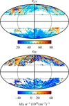 |
Fig. A.1 LV-correlated dust emissivity map (εLV; top) and IV-correlated dust emissivity map (εIV; bottom) obtained from the template-fit approach as discussed in Sect. 3. The εIV map is mostly noisy in the southern Galactic hemisphere. |
Appendix B Masks
The binary and apodised masks used in this work are shown in Fig. B.1.
 |
Fig. B.1 Binary mask (left) with inner 180 × 180 pixels and the 256 × 256 pixels apodised mask (right) used in our analysis. |
Appendix C Results for simulations
Appendix C.1 Synthetic contamination maps
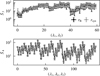 |
Fig. C.1 Same as Fig. 5 but for S̄3 and S̄4 statistics. The coefficients are obtained by averaging over angles. The grey crosses are shifted in the x-axis. |
In Fig. C.1 we present the normalised SC statistics (S̄3 and S̄4) for 25 rB regions and 300 rsyn maps, arranged in lexicographic order. As the contamination is independent of the wavelet orientations, the coefficients are averaged over angles. This demonstrates that the synthetic maps have identical SC statistics as the input contamination maps.
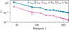 |
Fig. C.2 Angular power spectra Cℓ vs. ℓ for input and output maps, showing auto-spectra of ssim (cyan circles) and s̃sim (blue crosses) and cross-spectra with the NH I map (pink and red, respectively). |
Appendix C.2 Validating the component-separation algorithm
Figure C.2 shows the power spectra of the input and output dust maps. The spectra for ssim and s̃sim are consistent. We also successfully recovered the input correlation with the NH I map.
In Fig. C.3 we show the normalised SC statistics, S̄3 and S̄4, for msim, ssim and s̃sim in lexicographic order. The algorithm preserves the correlations between the different wavelet scales present in ssim. Here, although the maps are anisotropic, we averaged over angles to reduce the number of coefficients and improve readability.
Figure C.4 shows the SC statistics (S1, S2, S̄3, and S̄4) for msim, ssim and s̃sim at S/N = 5.
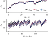 |
Fig. C.3 Comparison of S̄3 and S̄4 statistics between msim, ssim and s̃sim. To reduce the number of coefficients and improve readability, we average over angles. |
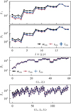 |
Fig. C.4 Summary statistics S1, S2, S̄3, and S̄4 for the S/N = 5 simulation case. |
Appendix D Statistics of the Planck contamination map
We compared the statistics of the recovered contamination map from SC-based component-separation method with the template-fit approach (discussed in Sect. 3) over the same Planck field as shown in Fig. 13. The histograms of the rB and r̃ are shown in Fig. D.1 over the whole field and over the central unmasked region. From the histogram plot, it is clear that rB is highly nonGaussian (independent of the mask) due to the presence of the Galactic residuals (dark gas, molecular H2 and ionised hydrogen). The distribution of r map is close to the Gaussian once we exclude the boundary pixels. The black dotted line in Fig. D.1 is the Gaussian fit to the distribution of r within the central unmasked region. Therefore, we can conclude that the SCbased component algorithm performs better than the template-fit approach in sky regions where excess H I-uncorrelated Galactic emissions are present. In Fig. D.2 we show the MFs of r̃ (dashed blue line), rB (solid red line) and those from the 300 rsyn maps (solid grey lines) within the binary mask. The MFs of the r map agree well with the 300 rsyn maps. Figures D.1 and D.2 demonstrate that the contamination map of the SC-based component-separation do not exhibit a non-Gaussian signature of Galactic emission.
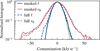 |
Fig. D.1 1D distributions of r̃ (blue) and rB (red). The solid lines show pixels within the binary mask and the dashed lines within the full region. The dotted black line is the Gaussian fit to the distribution of r̃ over the binary mask. |
Appendix E Comparison of the component-separated Planck data results
For completeness, we showed the results of the componentseparation algorithm for the Planck data region used to validate the component-separation algorithm in Sect. 7. Assuming the mean standard deviation of the contamination maps, σrsyn = 9.0k Jy sr−1, this specific sky patch in the Planck data has an S/N ≈ 5. The first column of Fig. E.1 shows md, second column shows s̃, and third column shows r̃, highlighting the difference between the Planck data and the recovered dust map. The first column of Fig. E.1 shows md, second column shows s̃, and third column shows r̃, highlighting the difference between md and s̃. The standard deviation of r̃ computed over the binary mask is 8.3kJy sr−1, consistent with the expected standard deviation of the 300 rsyn that are used as an input to the component-separation algorithm.
The bright infrared point source centred at Galactic coordinates (l, b) = (45.0°, −54.3°) is mostly present in the recovered dust map and a small fraction of it leaks into the residual map.
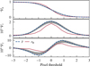 |
Fig. D.2 MFs of the r̃ (dashed blue line) and MFs of all 300 realisations of rsyn (grey lines). The three MFs of r̃ match well with the corresponding MFs of rsyn used as an input to the component-separation algorithm. The solid red line represents the MFs of the rB map obtained from the template-fit approach. |
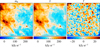 |
Fig. E.1 Planck data at 353 GHz (left), s̃ (middle), and r̃ (right) for the same sky region as used in Sect. 7. |
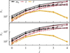 |
Fig. E.2 S1 and S2 coefficients of the md, s̃, and r̃ maps. The four line types show the four different orientations. |
We applied a 1° cut around the point source to exclude it from the further analysis of the summary statistics and the power spectrum. Figure E.2 shows the S1 and S2 coefficients for md, s̃ and r for the four different orientations of the wavelet. The md map at large scales (or high j values) is signal dominated. The contamination map, which is statistically isotropic, has roughly the same power in all four orientations.
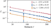 |
Fig. E.3 Auto spectrum Cℓ with ℓ of s̃ (red crosses) and the best-fit power-law model (red line) in units of kJy2 sr−1. The blue shows the cross power spectrum of s̃ and the NHI data along with the best-fit power-law model in kJy sr−1(1020 cm−2). The orange shows the auto spectrum of the total NHI data with the best-fit model in (1020 cm−2)2. |
Figure E.3 shows the power spectra of s̃ and the NHI data for the same region. We fitted the dust spectrum with the powerlaw model within the same multipole range as in Sect. 2.1. The straight lines in Fig. E.3 show the best-fit power-law models for the auto-power spectrum of s̃, cross-power spectrum of s with NHI map, and auto-power spectrum of the NHI map. The best-fit exponents are αs̃ = −2.51 ± 0.10, α× = −2.92 ± 0.15 and αHI = −2.84 ± 0.12, respectively. In this case, the difference in the slopes of s̃ and NHI spectra, Δα = αs̃ – αH I ≈ 0.3. We inferred that Δα ≠ 0 could be due to dust emission associated with H2.
In addition to the normalisation of the SC statistics described Eq. (6), we take here the log of the S1 and S2 coefficients.
All Figures
|
Fig. 1 Orthographic projection of the residual map obtained from the template-fit approach. The northern (southern) Galactic hemisphere is shown on the left (right). The white regions are masked from the analysis as they comprise NHI cut-off pixels and the pixels were masked due to iterative masking. |
| In the text | |
|
Fig. 2 Spatial distribution of the residual maps in the selected 25 square patches. |
| In the text | |
|
Fig. 3 Average power spectrum, in terms of ℓCℓ with multipole ℓ over all the 25 selected square patches (black points). The error bars on them are the standard deviation obtained on the spectra. The solid black line represents the best-fit CIB model by Lenz et al. (2019) at 353 GHz. |
| In the text | |
|
Fig. 4 Variation in V0, V1, and V2 with the pixel threshold of the MFs over all the 25 patches. The perimeter and Euler functions are scaled with 102 and 104, respectively, for visualisation purpose. The solid black line represents the MFs computed from the average of ten FFP10 noise-contaminated Gaussian CIB realisations over a given patch. |
| In the text | |
|
Fig. 5 Comparison of the S1 and S2 statistics of mean and standard deviation of 25 contamination maps obtained from the template-fit approach rB regions (black circles) and 300 synthetic contamination maps rsyn (grey crosses). The grey crosses are shifted in the x-axis. |
| In the text | |
|
Fig. 6 Top : input maps at S/N = 3 centred around the sky patch at (l, b) = (45.0°, −54.3°). The columns from left to right show the input dust map (ssim), the input contamination map (rsim), and the total simulated map (msim). Bottom : columns from left to right: Component-separated dust map (s̃sim), residual map (r̃sim), and difference between input and recovered dust map (δs). |
| In the text | |
|
Fig. 7 Top : ℓCℓ spectra for rsim (solid pink), r̃sim (dashed red), δs (dashed-dotted orange), and magnitude of the cross-spectrum for rsim and δs (dashed-dot-dotted blue) in kJy2sr−1. Bottom : cross-spectra (l2Cl) of δs (solid green) and r̃sim (dashed brown) with the NHI map, in kJy sr−1(1020cm−2). |
| In the text | |
|
Fig. 8 Top : s̃sim (left), HI column density map (middle), and the mean of 25 realisations of δs (right). Bottom : 2D correlation between NHI and 〈δs〉. The blue crosses and the error bars show the median values and standard deviations of mean 〈δs〉 in the ordered bins of NHI. |
| In the text | |
|
Fig. 9 Comparison of S1 and S2 statistics of msim (black circles), ssim (red circles), and the s̃sim (blue crosses with dashed line). |
| In the text | |
|
Fig. 10 Comparison of the angle-averaged S1 and S2 statistics of rsim (red circles) and r̃sim (blue crosses with the dashed line). The cyan squares with the dashed-dotted line show the cross coefficients between δs and r̃sim, and the orange diamonds with the dashed-dot-dotted line show that between rsim and r̃sim. |
| In the text | |
|
Fig. 11 Comparison of the angle-averaged S2 cross statistics with the NHI map: r̃sim (dashed blue) and the mean over 300 rsyn (black). The recovered contamination is consistent with the expected statistics within 1σ. The blue crosses are slightly shifted along the x-axis. The grey lines show all 300 rsyn realisations. |
| In the text | |
|
Fig. 12 2D histogram showing the joint distribution of ssim and NHI. The black circles correspond to the median values, and the upper and lower limits correspond to the 16 and 84 percentile of msim of the data in each ordered bin of NHI. Similarly, the red circles show ssim, and the blue crosses show s̃sim. |
| In the text | |
|
Fig. 13 Top : Planck 353 GHz map (CMB and global offset subtracted; left), r̃ (middle) and s̃ (right) after component-separation in the same sky region as in Fig. 6. Bottom : decomposed s̃HI (left) and s̃H2 maps (middle). The sCSFD map at 100 μm (in mag units) in the same sky region is shown in the right panel. |
| In the text | |
|
Fig. 14 Top : correlation plot of r̃ with NHI map. The blue data points and the error bars show the zero median and standard deviation of r̃ in the ordered bins of NHI. The standard deviations are consistent in all the NHI bins. Middle : comparison of angle-averaged S2 statistics of r̃ (red cross), rLSS (square dashed orange line) and the ensemble average of 300 rsyn maps (black circles) along with 1σ, 2σ, and 3σ error bands. Bottom : red crosses with the solid line show cross S2 coefficients between s̃ and r̃, and the blue circles with the dashed line show the cross S2 coefficients between s̃ and rLSS. The blue circles are slightly shifted in the x-axis. |
| In the text | |
|
Fig. 15 S1, S2, and S21/S2 for the s̃HI map (red circles) and the |
| In the text | |
|
Fig. A.1 LV-correlated dust emissivity map (εLV; top) and IV-correlated dust emissivity map (εIV; bottom) obtained from the template-fit approach as discussed in Sect. 3. The εIV map is mostly noisy in the southern Galactic hemisphere. |
| In the text | |
|
Fig. B.1 Binary mask (left) with inner 180 × 180 pixels and the 256 × 256 pixels apodised mask (right) used in our analysis. |
| In the text | |
|
Fig. C.1 Same as Fig. 5 but for S̄3 and S̄4 statistics. The coefficients are obtained by averaging over angles. The grey crosses are shifted in the x-axis. |
| In the text | |
|
Fig. C.2 Angular power spectra Cℓ vs. ℓ for input and output maps, showing auto-spectra of ssim (cyan circles) and s̃sim (blue crosses) and cross-spectra with the NH I map (pink and red, respectively). |
| In the text | |
|
Fig. C.3 Comparison of S̄3 and S̄4 statistics between msim, ssim and s̃sim. To reduce the number of coefficients and improve readability, we average over angles. |
| In the text | |
|
Fig. C.4 Summary statistics S1, S2, S̄3, and S̄4 for the S/N = 5 simulation case. |
| In the text | |
|
Fig. D.1 1D distributions of r̃ (blue) and rB (red). The solid lines show pixels within the binary mask and the dashed lines within the full region. The dotted black line is the Gaussian fit to the distribution of r̃ over the binary mask. |
| In the text | |
|
Fig. D.2 MFs of the r̃ (dashed blue line) and MFs of all 300 realisations of rsyn (grey lines). The three MFs of r̃ match well with the corresponding MFs of rsyn used as an input to the component-separation algorithm. The solid red line represents the MFs of the rB map obtained from the template-fit approach. |
| In the text | |
|
Fig. E.1 Planck data at 353 GHz (left), s̃ (middle), and r̃ (right) for the same sky region as used in Sect. 7. |
| In the text | |
|
Fig. E.2 S1 and S2 coefficients of the md, s̃, and r̃ maps. The four line types show the four different orientations. |
| In the text | |
|
Fig. E.3 Auto spectrum Cℓ with ℓ of s̃ (red crosses) and the best-fit power-law model (red line) in units of kJy2 sr−1. The blue shows the cross power spectrum of s̃ and the NHI data along with the best-fit power-law model in kJy sr−1(1020 cm−2). The orange shows the auto spectrum of the total NHI data with the best-fit model in (1020 cm−2)2. |
| In the text | |
Current usage metrics show cumulative count of Article Views (full-text article views including HTML views, PDF and ePub downloads, according to the available data) and Abstracts Views on Vision4Press platform.
Data correspond to usage on the plateform after 2015. The current usage metrics is available 48-96 hours after online publication and is updated daily on week days.
Initial download of the metrics may take a while.